Adaptive Temporal Compressive Sensing for Video

Abstract

This paper introduces the concept of adaptive temporal compressive sensing (CS) for video. We propose a CS algorithm to adapt the compression ratio based on the scene’s temporal complexity, computed from the compressed data, without compromising the quality of the reconstructed video. The temporal adaptivity is manifested by manipulating the integration time of the camera, opening the possibility to real-time implementation. The proposed algorithm is a generalized temporal CS approach that can be incorporated with a diverse set of existing hardware systems.

Index Terms—  Video compressive sensing, temporal compressive sensing ratio design, temporal superresolution, adaptive temporal compressive sensing, real-time implementation.

1 Introduction

Video compressive sensing (CS), a new application of CS, has recently been investigated to capture high-speed videos at low frame rate by means of temporal compression [1, 2, 3]. A commonality of these video CS systems is the use of per-pixel modulation during one integration time-period, to overcome the spatio-temporal resolution trade-off in video capture. As a consequence of active [1, 2] and passive pixel-level coding strategies [3, 9] (see Fig. 1), it is possible to uniquely modulate several temporal frames of a continuous video stream within the timescale of a single integration period of the video camera (using a conventional camera). This permits these novel imaging architectures to maintain high resolution in both the spatial and the temporal domains. Each low-speed exposure captured by such CS cameras is a linear combination of the underlying coded high-speed video frames. After acquisition, high-speed videos are reconstructed by various CS inversion algorithms [10, 11, 12, 13].

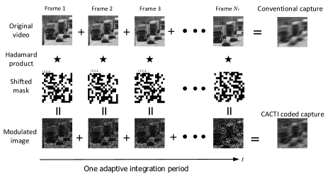
Fig. 1: Illustration of the coding mechanisms within the Coded Aperture Compressive Temporal Imaging (CACTI) system [3]. The first row shows $N_{F}$ high-speed temporal frames of the source datacube video; the second row depicts the mask with which each frame is multiplied (black is zero, white is one). In CACTI, the same code (mask) is shifted (from left to right) to constitute a series of frame-dependent codes. Finally, the CACTI measurement of these $N_{F}$ frames is the sum of the coded frames, as shown at right-bottom.

These hardware systems were originally designed for fixed temporal compression ratios. The correlation in time between video frames can vary, depending on the detailed time dependence of the scene being imaged. For example, a scene monitored by a surveillance camera may have significant temporal variability during the day, but at night there may be extended time windows with no or limited changes. Therefore, adapting the temporal compression ratio based on the captured scene is important, not only to maintain a high quality reconstruction, but also to save power, memory, and related resources.

We introduce the concept of adaptive temporal compressive sensing to manifest a CS video system that adapts to the complexity of the scene under test. Since each of the aforementioned cameras involves similar integration over a time window, in which $N_{F}$ high-speed video frames are modulated/coded, we propose to adapt this time window (the integration time $N_{F}$), to change the temporal compression ratio as a function of the complexity of the data. Specifically, we adaptively determine the number of frames $N_{F}$ collapsed to one measurement, using motion estimation in the compressed domain.

The algorithm for adaptive temporal CS can be incorporated with a diverse range of existing video CS systems (not only the imaging architectures in [1, 2, 3] but also flutter shutter [23, 24] cameras), to implement real-time temporal adaptation. Furthermore, thanks to the availability of hardware for simple motion estimation [25], the proposed algorithm can be readily implemented in these cameras.

2 Proposed Method

The underlying principle of the proposed method is to determine the temporal compression ratio $N_{F}$ based on the motion of the scene being sensed. In the following, we propose to estimate the motion of the objects within the scene, to adapt the compression ratio for effective video capture.

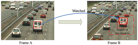
Fig. 2: Basic principle of block-matching. Search all the $P\times P$ blocks in the window of frame B to find the one best matched with the block in frame A, and use this to compute the block motion.

2.1 Block-Matching Motion Estimation

The block-matching method considered here has been employed in a variety of video codes ranging from MPEG1 / H.261 to MPEG4 / H.263 [25, 26, 27]. Diverse algorithms [26] have investigated the block-matching concept shown in Fig. 2. The key steps of the block-matching method are reviewed as follows: $i$) partition frame A (e.g., previous frame) into $P\times P$ (pixels) blocks; $ii$) pre-define a window size $M\times M$ (pixels); $iii$) search all the $P\times P$ blocks in the $M\times M$ windows in frame B (e.g., current frame) around the selected block in frame A; $iv$) and find the best-matching block in the window according to some metric (e.g. mean squared error), and use this to compute the block motion. We demonstrate adaptive compression ratios based on this estimated motion from reconstructed video frames in Section 3.

Estimating motion in high-speed dynamic scenes via the block-matching method in the reconstructed video (after signal recovery) is computationally infeasible given current reconstruction times at even modest compression ratios. Hence, we aim to compute the adaption of $N_{F}$ based directly on the raw (compressed) measurements without the intermediate step of reconstruction. The following section proposes a method to estimate motion solely on low-framerate, coded measurements from the camera.

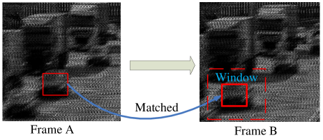
Fig. 3: Real-time motion estimation by block-matching.

2.2 Real-Time Block-Matching Motion Estimation

Estimating motion from the camera captured data requires the motion to be observable without reconstructing the video frames from the measurement. Fig. 3 presents the underlying principle of the real-time block-matching motion estimation approach. From this figure, it is apparent that the scene’s motion is observable within the time-integrated coding structure. This property lets us employ the block-matching method directly on raw measurements (frames A and B in Fig. 3) to estimate the scene’s motion. Adapting the compression ratio $N_{F}$ online is feasible due to the computational simplicity of this method.

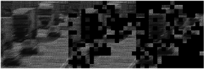
Fig. 4: Segmentation of foreground and background by motion estimation from compressed measurements. Left is the original measurement; middle is the background blocks with foreground blocks shown in black and the right part presents the foreground blocks with background blocks shown in black. Note that the aim of this work is to estimate the motion, not segmentation. This primary segmentation helps us to localize the moving parts of the scene. $16\times 16$ ($P=16$) blocksize is used and the window size is defined as $40\times 40$ ($M=40$). Cross-diamond search algorithm [28] has been used to generate this figure and the subsequent results in Section 3.

We may roughly segment the video sequence into foreground and background regions by computing the number of pixels that each block traverses between frames. For each block, if this number is greater than a pre-specified threshold, the block is presumably moving and is hence classified as foreground. Other blocks are considered background (Fig. 4). Notably, we adapt $N_{F}$ solely based on the estimated motion velocity $V$ (pixels/frame) for the blocks determined by the block matching algorithm to have moved the greatest number of pixels between frames.

Intuitively, the compression ratio required to faithfully reconstruct the scene’s motion is inversely proportional to the detected velocity $V$, reaching a finite upper bound as $V\rightarrow 0$. In practice, we simply apply a look-up table to (discretely) appropriately adapt $N_{F}$ with few computations. See Table 1 for an example. Since good hardware exists for motion estimation [25] , the proposed method can be implemented in real time.

It is worth noting that the estimated motion (and hence the compression ratio determined by the look-up table) are used in the upcoming frames. We assume the consistent motion of the adjacent frames in the video. Sudden changes of the motion will result in one integration time delay of the $N_{F}$ adaption. Simulation results in Fig. 5 verify this point. We can of course put an upper bound in $N_{F}$.

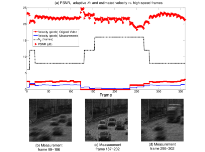
Fig. 5: (a) Reconstruction PSNR (dB), adaptive $N_{F}$ (frames), and velocities (pixels/frame) estimated from the original video and measurements, all are plotted against frame number. (b-d) Measurements with vehicles at different velocities.

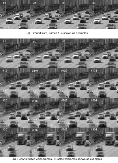
Fig. 6: Selected reconstructed frames (b) based on the adaptive $N_{F}$ presented in Fig. 5. Frames 1 to 4 in (a) are shown as examples of ground truth.

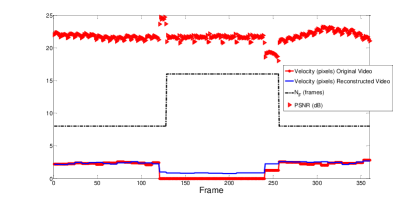
Fig. 7: Reconstruction PSNR (dB), adaptive $N_{F}$ (frames), and velocities (pixels/frame) estimated from the original and reconstructed video frames, all are plotted against frame number.

$V$	$[0,0.5)$	$[0.5,1)$	$[1,2)$	$[2,3)$	$[3,7)$	$\geq$ 7
$N_{F}$	16	12	8	6	4	2

Table 1: Relationships between the velocity $V$ (pixels/frame) of the foreground and the compression ratio $N_{F}$ (frames).

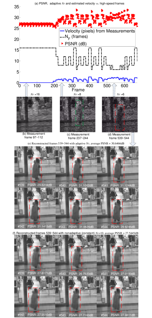
Fig. 8: Motion estimation and adaptive $N_{F}$ from the measurements. (a) Reconstruction PSNR (dB), adaptive $N_{F}$ (frames) (average adaptive $N_{F}$=10.12), and velocities (pixels/frame) estimated from the measurements, all are plotted against frame number. (b-d) Measurements when there is nothing, one person, and a couple moving inside the scene, adapted $N_{F}=16,8,6$, respectively. (e) Reconstructed frames 539-544 from the measurement in (d) with adaptive $N_{F}$. (f) Reconstructed frames 539-544 with nonadpative (constant) $N_{F}=10$.

3 Experimental Results

From [3], we have found that (based on extensive simulations) shifting a fixed mask is as good as using the more sophisticated time evolving codes used in [1, 2]. For convenience (but not necessity), the subsequent results will use a shifted mask to modulate the high-speed video frames.

3.1 Example 1: Synthetic Traffic Video

We illustrate the adaptive compression ratio framework on a traffic video [29] that has 360 frames. We artificially vary the foreground velocity for this video to evaluate the proposed method’s performance for motion estimation and $N_{F}$ adaption. Frames 1-120 (Fig. 5(b)) and 241-336 (Fig. 5(d)) run at the originally-captured framerate; we freeze the scene between frames 121-240 (Fig. 5(c)). The generalized alternating projection (GAP) algorithm [12] is used for the reconstructions.

Table 1 provides the compression ratio $N_{F}$ corresponding to several scene velocities $V$. This look-up table (learned based on training data) seeks to maintain a constant reconstruction peak signal-to-noise ratio (PSNR) of 22dB. Fig. 5 presents the real-time motion estimation results using simulated low-framerate coded exposures of the traffic video with an initial compression ratio $N_{F}=6$. After a short fluctuation, the estimated velocity of the scene becomes constant; $N_{F}$ accordingly stabilizes at 8. When the vehicles freeze, the block-matching algorithm senses zero change in the pixel position and updates $N_{F}$ to 16. $N_{F}$ returns to 8 upon continuing video playback at normal speed. We can also observe the consistence of velocities estimated from the original video and from the compressed measurements in Fig. 5(a). Sudden changes in the video’s framerate (and hence the motion velocity $V$) are reflected in short fluctuations of the PSNR (for one time-integration period) in Fig. 5(a). The average PSNR of the reconstructed frames in Fig. 5 is 21.8dB, very close to our expectation (22dB). Fig. 6 presents several reconstructed frames based on the adaptive $N_{F}$ in Fig. 5.

We additionally evaluate the block-matching algorithm’s performance by deploying it to reconstructed frames. Fig. 7 demonstrates that its performance is similar to the phenomena shown in Fig. 5. This justifies that it is unnecessary to reconstruct each measurement prior to updating $N_{F}$.

3.2 Example 2: Realistic Surveillance Video

Fig. 8 implements adaptive $N_{F}$ on video data captured in front of a shop [30]. Table 1 is again useful for this example.

The first 189 frames of this video (Fig. 8(b)) are stationary; nothing is moving within the scene. As seen before, since $V=0$, the compression ratio remains at $N_{F}$=16. After the 189^th frame, different people begin to walk in and out of the video area (Fig. 8(c-d)). The compression ratio $N_{F}$ is adapted between 6 and 16 according to the estimated velocity. When one person walks into the shop (Fig. 8(c)), the compression ratio drops ($N_{F}$=8). This results in a better-posed reconstruction of the underlying video frames. When a couple walks in front of the shop (Fig. 8(d)), $N_{F}$ drops further to 6. The corresponding measurement and reconstructed frames are shown in Fig. 8(d,e).

This video takes a total of 67 adaptive measurements to capture and reconstruct 678 high-speed video frames, achieving a mean compression ratio $N_{F}\approx$10.12. To demonstrate the utility of adapting $N_{F}$ based on the sensed data, we compare adaptive reconstructions to those obtained when $N_{F}$ is fixed at or near its expected value. Fig. 8(f) shows reconstructed frames 539-544 when fixing $N_{F}$ = 10. Comparing part (e) with part (f), we notice that adapting $N_{F}$ provides a (3dB) higher reconstruction quality (average PSNR=30.65dB) than fixing $N_{F}$ near its expected value (average PSNR=27.54dB). These improvements are most noticeable whenever there is motion within the scene and demonstrate the potency of temporal compression ratio adaptation in realistic applications.

4 Conclusion

We have introduced the concept of adaptive temporal compressive sensing for video and demonstrated a real-time method to adjust the temporal compression ratio for video compressive sensing. By estimating the motion of objects within the scene, we determine how many measurements are necessary to ensure a reasonably well-conditioned estimation of high-speed motion from lower-framerate measurements.

A block-matching algorithm estimates the scene’s motion directly from the compressed measurements to obviate real-time reconstruction, thereby significantly reducing the expended real-time computational resources. Simulation results have verified the efficacy of the proposed adaption algorithm. Future work will seek to embed this real-time framework into the hardware prototype.

References

- [1] Y. Hitomi, J. Gu, M. Gupta, T. Mitsunaga, and S. K. Nayar, “Video from a single coded exposure photograph using a learned over-complete dictionary,” IEEE International Conference on Computer Vision (ICCV), pp. 287–294, November 2011.
- [2] D. Reddy, A. Veeraraghavan, and R. Chellappa, “P2C2: Programmable pixel compressive camera for high speed imaging,” IEEE International Conference on Computer Vision and Pattern Recognition (CVPR), pp. 329–336, June 2011.
- [3] P. Llull, X. Liao, X. Yuan, J. Yang, D. Kittle, L. Carin, G. Sapiro, and D. J. Brady, “Coded aperture compressive temporal imaging,” Optics Express, vol. 21, no. 9, pp. 10526–10545.
- [4] A. C. Sankaranarayanan, P. K. Turaga, R. G. Baraniuk, and R. Chellappa, “Compressive acquisition of dynamic scenes,” 11th European Conference on Computer Vision, Part I, pp. 129–142, September 2010.
- [5] A. C. Sankaranarayanan, C. Studer, and R. G. Baraniuk, “CS-MUVI: Video compressive sensing for spatial-multiplexing cameras,” IEEE International Conference on Computational Photography, pp. 1–10, April 2012.
- [6] M. B. Wakin, J. N. Laska, M. F. Duarte, D. Baron, S. Sarvotham, D. Takhar, K. F. Kelly, and R. G. Baraniuk, “Compressive imaging for video representation and coding,” Proceedings of the Picture Coding Symposium, pp. 1–6, April 2006.
- [7] M. F. Duarte, M. A.Davenport, D. Takhar, and S. Ting J. N. Laska, K. F. Kelly, and R. G. Baraniuk, “Single-pixel imaging via compressive sampling,” IEEE Signal Processing Magazine, vol. 25, no. 2, pp. 83–91, March 2008.
- [8] A. Veeraraghavan, D. Reddy, and R. Raskar, “Coded strobing photography: Compressive sensing of high speed periodic videos,” IEEE Transactions on Pattern Analysis and Machine Intelligence, vol. 33, no. 4, pp. 671–686, April 2011.
- [9] P. Llull, X. Liao, X. Yuan, J. Yang, D. Kittle, L. Carin, G. Sapiro, and D. J. Brady, “Compressive sensing for video using a passive coding element,” Computational Optical Sensing and Imaging, 2013.
- [10] J. A. Tropp and A. C. Gilbert, “Signal recovery from random measurements via orthogonal matching pursuit,” IEEE Transactions on Information Theory, vol. 53, no. 12, pp. 4655–4666, December 2007.
- [11] J.M. Bioucas-Dias and M.A.T. Figueiredo, “A new TwIST: Two-step iterative shrinkage/thresholding algorithms for image restoration,” IEEE Transactions on Image Processing, vol. 16, no. 12, pp. 2992–3004, December 2007.
- [12] X. Liao, H. Li, and L. Carin, “Generalized alternating projection for weighted- minimization with applications to model-based compressive sensing,” accepted to appear in SIAM Journal on Imaging Sciences, 2012.
- [13] J. Yang, X. Yuan, X. Liao, P. Llull, G. Sapiro, D. J. Brady, and L. Carin, “Gaussian mixture model for video compressive sensing,” International Conference on Image Processing, 2013.
- [14] M. Elad, “Optimized projections for compressed sensing,” IEEE Transactions on Signal Processing, vol. 55, no. 12, pp. 5695–5702, December 2007.
- [15] S. Ji, Y. Xue, and L. Carin, “Bayesian compressive sensing,” IEEE Transactions on Signal Processing, vol. 56, no. 6, pp. 2346–2356, June 2008.
- [16] W. Carson, M. Chen, M. Rodrigues, R. Calderbank, and L. Carin, “Communications inspired projection design with application to compressive sensing,” SIAM Journal on Imaging Sciences, vol. 5, no. 4, pp. 1185–1212, 2012.
- [17] J. M. Duarte-Carvajalino, G. Yu, L. Carin, and G. Sapiro, “Task-driven adaptive statistical compressive sensing of gaussian mixture models,” IEEE Transactions on Signal Processing, vol. 61, no. 3, pp. 585–600, February 2013.
- [18] L. Zelnik-Manor, K. Rosenblum, and Y. C. Eldar, “Sensing matrix optimization for block-sparse decoding,” IEEE Transactions on Signal Processing, vol. 59, no. 9, pp. 4300–4312, September 2011.
- [19] Z. Liu, A. Y. Elezzabi, and H. V. Zhao, “Maximum frame rate video acquisition using adaptive compressed sensing,” IEEE Transactions on Circuits and Systems for Video Technology, vol. 21, no. 11, pp. 1704–1718, November 2011.
- [20] J. Y. Park and M. B. Wakin, “A multiscale framework for compressive sensing of video,” Proceedings of the Picture Coding Symposium, pp. 1–4, May 2009.
- [21] M. Azghani, A. Aghagolzadeh, and M. Aghagolzadeh, “Compressed video sensing using adaptive sampling rate,” International Symposium on Telecommunications, pp. 710–714, 2010.
- [22] J. E. Fowler, S. Mun, and E. W. Tramel, “Block-based compressed sensing of images and video,” Foundations and Trends in Signal Processing, vol. 4, no. 4, pp. 297–416, 2012.
- [23] R. Raskar, A. Agrawal, and J. Tumblin, “Coded exposure photography: motion deblurring using fluttered shutter,” ACM Transactions on Graphics, vol. 25, no. 3, pp. 795, 2006.
- [24] Y. Tendero, J-M Morel, and B. Rougé, “The flutter shutter paradox,” to appear in SIAM Journal on Imaging Sciences, pp. 1–33, 2013.
- [25] C.-H. Hsieh and T.-P. Lin, “VLSI architecture for block-matching motion estimation algorithm,” IEEE Transactions on Circuits and Systems for Video Technology, vol. 2, no. 2, pp. 169–175, June 1992.
- [26] M. Ezhilarasan and P. Thambidurai, “Simplified block matching algorithm for fast motion estimation in video compression,” Journal of Computer Science, vol. 4, no. 4, pp. 282–289, 2008.
- [27] D. J. Le Gall, “The MPEG video compression algorithm,” Signal Processing: Image Communication, vol. 4, no. 2, pp. 129–140, April 1992.
- [28] C.-H. Cheung and L.-M. Po, “A novel cross-diamond search algorithm for fast block motion estimation,” IEEE Transactions on Circuits and Systems for Video Technology, vol. 12, no. 12, pp. 1168–1177, December 2002.
- [29] “http://projects.cwi.nl/dyntex/database_pro.html,” .
- [30] “http://i21www.ira.uka.de/image_sequences/,” .