The classical ether-drift experiments:
a modern re-interpretation

M. Consoli^(a), C. Matheson^(b) and A. Pluchino ^(a,c)

a) Istituto Nazionale di Fisica Nucleare, Sezione di Catania, Italy

b) Selwyn College, Cambridge, United Kingdom

c) Dipartimento di Fisica e Astronomia dell’Università di Catania, Italy

Abstract

The condensation of elementary quanta and their macroscopic occupation of the same quantum state, say ${\bf k}=0$ in some reference frame $\Sigma$, is the essential ingredient of the degenerate vacuum of present-day elementary particle physics. This represents a sort of ‘quantum ether’ which characterizes the physically realized form of relativity and could play the role of preferred reference frame in a modern re-formulation of the Lorentzian approach. In spite of this, the so called ‘null results’ of the classical ether-drift experiments, traditionally interpreted as confirmations of Special Relativity, have so deeply influenced scientific thought as to prevent a critical discussion on the real reasons underlying its alleged supremacy. In this paper, we argue that this traditional null interpretation is far from obvious. In fact, by using Lorentz transformations to connect the Earth’s frame to $\Sigma$, the small observed effects point to an average Earth’s velocity of about 300 km/s, as in most cosmic motions. A common feature is the irregular behaviour of the data. While this has motivated, so far, their standard interpretation as instrumental artifacts, our new re-analysis of the very accurate Joos experiment gives clear indications for the type of Earth’s motion associated with the CMB anisotropy and leaves little space for this traditional interpretation. The new explanation requires instead a view of the vacuum as a stochastic medium, similar to a fluid in a turbulent state of motion, in agreement with basic foundational aspects of both quantum physics and relativity. The overall consistency of this picture with the present experiments with vacuum optical resonators and the need for a new generation of dedicated ether-drift experiments are also emphasized.

PACS: 03.30.+p; 01.55.+b; 11.30.Cp

1. Introduction

An analysis of the ether-drift experiments, starting from the original Michelson-Morley experiment of 1887, should be suitably framed within a general discussion of the basic differences between Einstein’s Special Relativity [1] and the Lorentzian point of view [2, 3, 4]. There is no doubt that the former interpretation is today widely accepted. However, in spite of the deep conceptual differences, it is not obvious how to distinguish experimentally between the two formulations. This type of conclusion was, for instance, already clearly expressed by Ehrenfest in his lecture ‘On the crisis of the light ether hypothesis’ (Leyden, December 1912) as follows: “So, we see that the ether-less theory of Einstein demands exactly the same here as the ether theory of Lorentz. It is, in fact, because of this circumstance, that according to Einstein’s theory an observer must observe exactly the same contractions, changes of rate, etc. in the measuring rods, clocks, etc. moving with respect to him as in the Lorentzian theory. And let it be said here right away and in all generality. As a matter of principle, there is no experimentum crucis between the two theories”. This can be understood since, independently of all interpretative aspects, the basic quantitative ingredients, namely Lorentz transformations, are the same in both formulations. Their validity will be assumed in the following to discuss the possible existence of a preferred reference frame.

For a modern presentation of the Lorentzian philosophy one can then refer to Bell [5, 6, 7]. In this alternative approach, differently from the usual derivations, one starts from physical modifications of matter (namely Larmor’s time dilation and Lorentz-Fitzgerald length contraction in the direction of motion) to deduce Lorentz transformations. In this way, due to the fundamental group properties, the relation between two observers $S^{\prime}$ and $S^{\prime\prime}$, individually related to the preferred frame $\Sigma$ by Lorentz transformations with dimensionless parameters $\beta^{\prime}=v^{\prime}/c$ and $\beta^{\prime\prime}=v^{\prime\prime}/c$, is also a Lorentz transformation with relative velocity parameter $\beta_{\rm rel}$ fixed by the relativistic composition rule

$$\beta_{\rm rel}={{\beta^{\prime}-\beta^{\prime\prime}}\over{1-\beta^{\prime}\beta^{\prime\prime}}}$$ (1)

(for simplicity we restrict to the case of one-dimensional motion). This produces a substantial quantitative equivalence with Einstein’s formulation for most standard experimental tests where one just compares the relative measurements of a pair of observers. Hence the importance of the ether-drift experiments where one attempts to measure an absolute velocity.

At the same time, if the velocity of light $c_{\gamma}$ propagating in the various interferometers coincides with the basic parameter $c$ entering Lorentz transformations, relativistic effects conspire to make undetectable the individual $\beta^{\prime}$, $\beta^{\prime\prime}$,…This means that a null result of the ether-drift experiments should not be automatically interpreted as a confirmation of Special Relativity. As stressed by Ehrenfest, the motion with respect to $\Sigma$ might remain unobservable, yet one could interpret relativity ‘ à la Lorentz’. This could be crucial, for instance, to reconcile faster-than-light signals with causality [8] and thus provide a different view of the apparent non-local aspects of the quantum theory [9].

However, to a closer look, is it really impossible to detect the motion with respect to $\Sigma$? This possibility, which was implicit in Lorentz’ words [4] “…it seems natural not to assume at starting that it can never make any difference whether a body moves through the ether or not..”, may induce one to re-analyze the classical ether-drift experiments. Let us first give some general theoretical arguments that could motivate this apparently startling idea.

A possible observation is that Lorentz symmetry might not be an exact symmetry. In this case, one could conceivably detect the effects of absolute motion. For instance Lorentz symmetry could represent an ‘emergent’ phenomenon and thus reflect the existence of some underlying form of ether. This is an interesting conceptual possibility which, in many different forms, objectively reflects the fast growing interest of part of the physics community, a partial list including i) the idea of the vacuum as a quantum liquid [10, 11] (which can explain in a natural way the huge difference between the typical vacuum-energy scales of modern particle physics and the cosmological term needed in Einstein’s equations to fit the observations) ii) the idea of Lorentz symmetry as associated with an infrared fixed point [12, 13] in non-symmetric quantum field theories iii) the quantum-gravity literature which, by starting from the original concept [14] of ‘space-time foam’, explicitly models the vacuum as a turbulent fluid [15, 16, 17] iv) the idea of deformations of Lorentz symmetry in a theoretical scheme (‘Doubly Special Relativity’) [18, 19, 20] where besides an invariant speed there is also an invariant length associated with the Planck scale v) the representation of relativistic particle propagation from the superposition, at very short time scales, of non-relativistic particle paths with different Newtonian mass [21].

Here, however, we shall adopt a different perspective and concentrate our analysis on a peculiar aspect of today’s quantum field theories: the representation of the vacuum as a ‘condensate’ of elementary quanta. These condense because their trivially empty vacuum is a meta-stable state and not the true ground state of the theory. In the physically relevant case of the Standard Model of electroweak interactions, this situation can be summarized by saying [22] that “What we experience as empty space is nothing but the configuration of the Higgs field that has the lowest possible energy. If we move from field jargon to particle jargon, this means that empty space is actually filled with Higgs particles. They have Bose condensed”. The explicit translation from field jargon to particle jargon, with the substantial equivalence between the effective potential of quantum field theory and the energy density of a dilute particle condensate, can be found for instance in ref.[23].

The trivial empty vacuum will eventually be re-established by heating the system above a critical temperature $T=T_{c}$ where the condensate ‘evaporates’. This temperature in the Standard Model is so high that one can safely approximate the ordinary vacuum as a zero-temperature system (think of ⁴He at a temperature $10^{-12}$ ^oK). This observation allows one to view the physical vacuum as a superfluid medium [10] where bodies can flow without any apparent friction, consistently with the experimental results. Clearly, this form of quantum vacuum is not the kind of ether imagined by Lorentz. However, if possible, this modern view of the vacuum state is even more different from the empty space-time of Special Relativity that Einstein had in mind in 1905. Therefore, one might ask [24] if Bose condensation, i.e. the macroscopic occupation of the same quantum state, say ${\bf{k}}=0$ in some reference frame $\Sigma$, can represent the operative construction of a ‘quantum ether’. This characterizes the physically realized form of relativity and could play the role of the preferred reference frame in a modern Lorentzian approach.

Usually this possibility is not considered with the motivation, perhaps, that the average properties of the condensed phase are summarized into a single quantity which transforms as a world scalar under the Lorentz group, for instance, in the Standard Model, the vacuum expectation value $\langle\Phi\rangle$ of the Higgs field. However, this does not imply that the vacuum state itself has to be Lorentz invariant. Namely, Lorentz transformation operators $\hat{U}^{\prime}$, $\hat{U}^{\prime\prime}$,..might transform non trivially the reference vacuum state $|\Psi^{(0)}\rangle$ (appropriate to an observer at rest in $\Sigma$) into $|\Psi^{\prime}\rangle$, $|\Psi^{\prime\prime}\rangle$,.. (appropriate to moving observers $S^{\prime}$, $S^{\prime\prime}$,..) and still, for any Lorentz-invariant operator $\hat{G}$, one would find

$$\langle\hat{G}\rangle_{\Psi^{(0)}}=\langle\hat{G}\rangle_{\Psi^{\prime}}=\langle\hat{G}\rangle_{\Psi^{\prime\prime}}=..$$ (2)

Here, we are assuming the existence of a suitable operatorial representation of the Poincaré algebra for the quantum theory in terms of 10 generators $P_{\alpha}$, $M_{\alpha,\beta}$ ( $\alpha$ ,$\beta$=0, 1, 2, 3) where $P_{\alpha}$ are the 4 generators of the space-time translations and $M_{\alpha\beta}=-M_{\beta\alpha}$ are the 6 generators of the Lorentzian rotations with commutation relations

$$[P_{\alpha},P_{\beta}]=0$$ (3)

$$[M_{\alpha\beta},P_{\gamma}]=\eta_{\beta\gamma}P_{\alpha}-\eta_{\alpha\gamma}P_{\beta}$$ (4)

$$[M_{\alpha\beta},M_{\gamma\delta}]=\eta_{\alpha\gamma}M_{\beta\delta}+\eta_{\beta\delta}M_{\alpha\gamma}-\eta_{\beta\gamma}M_{\alpha\delta}-\eta_{\alpha\delta}M_{\beta\gamma}$$ (5)

where $\eta_{\alpha\beta}={\rm diag}(1,-1,-1,-1)$.

With these premises, the possibility of a Lorentz-non-invariant vacuum state was addressed in refs.[25, 26] by comparing two basically different approaches. In the first description, as in the axiomatic approach to quantum field theory [27], one could describe the physical vacuum as an eigenstate of the energy-momentum vector. This physical vacuum state $|\Psi^{(0)}\rangle$ would maintain both zero momentum and zero angular momentum, i.e. (i,j=1,2,3)

$$\hat{P}_{i}|\Psi^{(0)}\rangle=\hat{M}_{ij}|\Psi^{(0)}\rangle=0$$ (6)

but, at the same time, be characterized by a non-vanishing energy

$$\hat{P}_{0}|\Psi^{(0)}\rangle=E_{0}|\Psi^{(0)}\rangle$$ (7)

This vacuum energy might have different explanations. Here, we shall limit ourselves to exploring the physical implications of its existence by just observing that, in interacting quantum field theories, there is no known way to ensure consistently the condition $E_{0}=0$ without imposing an unbroken supersymmetry, which is not phenomenologically acceptable. In this framework, by using the Poincaré algebra of the boost and energy-momentum operators, one then deduces that the physical vacuum cannot be a Lorentz-invariant state and that, in any moving frame, there should be a non-zero vacuum spatial momentum $\langle{\hat{P}_{i}}\rangle_{\Psi^{\prime}}\neq 0$ along the direction of motion. In this way, for a moving observer $S^{\prime}$ the physical vacuum would look like some kind of ethereal medium for which, in general, one can introduce a momentum density $\langle\hat{W}_{0i}\rangle_{\Psi^{\prime}}$ through the relation (i=1,2,3)

$$\langle{\hat{P}_{i}}\rangle_{\Psi^{\prime}}\equiv\int d^{3}x~{}\langle\hat{W}_{0i}\rangle_{\Psi^{\prime}}\neq 0$$ (8)

On the other hand, there is an alternative approach where one tends to consider the vacuum energy $E_{0}$ as a spurious concept and only concentrate on an energy-momentum tensor of the following form [28, 29]

$$\langle\hat{W}_{\mu\nu}\rangle_{\Psi^{(0)}}=\rho_{v}~{}\eta_{\mu\nu}$$ (9)

($\rho_{v}$ being a space-time independent constant). In this case, one is driven to completely different conclusions since, by introducing the Lorentz transformation matrices $\Lambda^{\mu}_{\nu}$ to any moving frame $S^{\prime}$, defining $\langle\hat{W}_{\mu\nu}\rangle_{\Psi^{\prime}}$ through the relation

$$\langle\hat{W}_{\mu\nu}\rangle_{\Psi^{\prime}}=\Lambda^{\sigma}{{}_{\mu}}\Lambda^{\rho}{{}_{\nu}}~{}\langle\hat{W}_{\sigma\rho}\rangle_{\Psi^{(0)}}$$ (10)

and using Eq.(9), it follows that the expectation value of $\hat{W}_{0i}$ in any boosted vacuum state $|\Psi^{\prime}\rangle$ vanishes, just as it vanishes in $|\Psi^{(0)}\rangle$, i.e.

$$\int d^{3}x~{}\langle\hat{W}_{0i}\rangle_{\Psi^{\prime}}\equiv\langle{\hat{P}_{i}}\rangle_{\Psi^{\prime}}=0$$ (11)

As discussed in ref.[25], both alternatives have their own good motivations and it is not so obvious how to decide between Eq.(8) and Eq.(11) on purely theoretical grounds. For instance, in a second-quantized formalism, single-particle energies $E_{1}({\bf{p}})$ are defined as the energies of the corresponding one-particle states $|{\bf{p}}\rangle$ minus the energy of the zero-particle, vacuum state. If $E_{0}$ is considered a spurious concept, $E_{1}({\bf{p}})$ will also become an ill-defined quantity. At a deeper level, one should also realize that in an approach based solely on Eq.(9) the properties of $|\Psi^{(0)}\rangle$ under a Lorentz transformation are not well defined. In fact, a transformed vacuum state $|\Psi^{\prime}\rangle$ is obtained, for instance, by acting on $|\Psi^{(0)}\rangle$ with the boost generator $\hat{M}_{01}$. Once $|\Psi^{(0)}\rangle$ is considered an eigenstate of the energy-momentum operator, one can definitely show [25] that, for $E_{0}\neq 0$, $|\Psi^{\prime}\rangle$ and $|\Psi^{(0)}\rangle$ differ non-trivially. On the other hand, if $E_{0}=0$ there are only two alternatives: either $\hat{M}_{01}|\Psi^{(0)}\rangle=0$, so that $|\Psi^{\prime}\rangle=|\Psi^{(0)}\rangle$, or $\hat{M}_{01}|\Psi^{(0)}\rangle$ is a state vector proportional to $|\Psi^{(0)}\rangle$, so that $|\Psi^{\prime}\rangle$ and $|\Psi^{(0)}\rangle$ differ by a phase factor.

Therefore, if the structure in Eq.(9) were really equivalent to the exact Lorentz invariance of the vacuum, it should be possible to show similar results, for instance that such a $|\Psi^{(0)}\rangle$ state can remain invariant under a boost, i.e. be an eigenstate of

$$\hat{M}_{0i}=-i\int d^{3}x~{}(x_{i}\hat{W}_{00}-x_{0}\hat{W}_{0i})$$ (12)

with zero eigenvalue. As far as we can see, there is no way to obtain such a result by just starting from Eq.(9) (this only amounts to the weaker condition $\langle\hat{M}_{0i}\rangle_{\Psi^{(0)}}=0$). Thus, independently of the finiteness of $E_{0}$, it should not come as a surprise that one can run into contradictory statements once $|\Psi^{(0)}\rangle$ is instead characterized by means of Eqs.(6)$-$(7). For these reasons, it is not obvious that the local relations (9) represent a more fundamental approach to the vacuum.

Alternatively, one could argue that a satisfactory solution of the vacuum-energy problem lies definitely beyond flat space. A non-zero $\rho_{v}$, in fact, should induce a cosmological term in Einstein’s field equations and a non-vanishing space-time curvature which anyhow dynamically breaks global Lorentz symmetry. Nevertheless, in our opinion, in the absence of a consistent quantum theory of gravity, physical models of the vacuum in flat space can be useful to clarify a crucial point that, so far, remains obscure: the huge renormalization effect which is seen when comparing the typical vacuum-energy scales of modern particle physics with the experimental value of the cosmological term needed in Einstein’s equations to fit the observations. For instance, as anticipated, the picture of the vacuum as a superfluid can explain in a natural way why there might be no non-trivial macroscopic curvature in the equilibrium state where any liquid is self-sustaining [10]. In any liquid, in fact, curvature requires deviations from the equilibrium state. The same happens for a crystal at zero temperature where all lattice distortions vanish and electrons can propagate freely as in a perfect vacuum. In such representations of the lowest energy state, where large condensation energies (of the liquid and of the crystal) play no observable role, one can intuitively understand why curvature effects can be orders of magnitude smaller than those naively expected by solving Einstein’s equations with the full $\langle\hat{W}_{\mu\nu}\rangle_{\Psi^{(0)}}$ as a cosmological term. In this perspective, ‘emergent-gravity’ approaches [30, 31, 32], where gravity somehow arises from the same physical flat-space vacuum, may become natural and, to find the effective form for the cosmological term to be inserted in Einstein’s field equations, we are lead to sharpen our understanding of the vacuum structure and of its excitation mechanisms by starting from the physical picture of a superfluid medium. To decide between Eqs.(8) and (11), one could then work out the possible observable consequences and check experimentally the existence of a fundamental energy-momentum flow.

2. Vacuum energy-momentum flow as an ether drift

To explore the idea of a non-zero vacuum energy-momentum flow, one can adopt a phenomenological model [25] where the physical vacuum is described as a relativistic fluid [34]. In this representation, a non-zero $\langle\hat{W}_{0i}\rangle_{\Psi^{\prime}}$ gives rise to a tiny heat flow and an effective thermal gradient in a moving frame $S^{\prime}$. This would represent a fundamental perturbation which, if present, is likely too small to be detectable in most experimental conditions by standard calorimetric devices. However, it could eventually be detected through very accurate ether-drift experiments performed in forms of matter that react by producing convective currents in the presence of arbitrarily small thermal gradients, i.e. in gaseous systems.

To better explain this possibility, let us first recall that in the modern version of these experiments one looks for a possible anisotropy of the two-way velocity of light through the relative frequency shift $\Delta\nu(\theta)$ of two orthogonal optical cavities [35, 36]. Their frequency

$$\nu(\theta)={{\bar{c}_{\gamma}(\theta)m}\over{2L(\theta)}}$$ (13)

is proportional to the two-way velocity of light $\bar{c}_{\gamma}(\theta)$ within the cavity through an integer number $m$, which fixes the cavity mode, and the length of the cavity $L(\theta)$ as measured in the laboratory. In principle, by filling the resonating cavities with some gaseous medium, the existence of a vacuum energy-momentum flow could produce two basically different effects:

a) modifications of the solid parts of the apparatus. These can change the cavity length upon active rotations of the apparatus or under the Earth’s rotation.

b) convective currents of the gas molecules inside the optical cavities. These can produce an anisotropy of the two-way velocity of light. In this sense, the reference frame $S^{\prime}$ where the solid container of the gas is at rest would not define a true state of rest.

Now, an anisotropy of the cavity length, in the laboratory frame, would amount to an anisotropy of the basic atomic parameters, a possibility which is severely limited experimentally. In fact, in the most recent versions of the original Hughes-Drever experiment [37, 38], where one measures the atomic energy levels as a function of their orientation with respect to the fixed stars, possible deviations from isotropy have been found below the $10^{-20}$ level [39]. This is incomparably smaller than any other effect on the velocity of light that we are going to discuss. Therefore, mechanism a), if present, is completely negligible and, from now on, we shall assume $L(\theta)=L=$constant. In this way, one re-obtains the standard relation adopted in the analysis of the experiments

$${{\Delta\nu^{\rm phys}(\theta)}\over{\nu_{0}}}={{\bar{c}_{\gamma}(\pi/2+\theta)-\bar{c}_{\gamma}(\theta)}\over{c}}\equiv{{\Delta\bar{c}_{\theta}}\over{c}}$$ (14)

where $\nu_{0}$ is the reference frequency of the two optical resonators and the suffix “${\rm phys}$” indicates a hypothetical physical part of the frequency shift after subtraction of all spurious effects.

Let us now estimate the possible effects of mechanism b) by first recalling that rigorous treatments of light propagation in dielectric media are based on the extinction theory [40]. This was originally formulated for continuous media where the inter-particle distance is smaller than the light wavelength. In the opposite case of an isotropic, dilute random medium [41] as a gas, it is relatively easy to compute the scattered wave in the forward direction and obtain the refractive index. However, the presence of convective currents would produce an anisotropy of the velocity of refracted light.

To derive the relevant relations, let us introduce from scratch the refractive index ${\cal N}$ of the gas. By assuming isotropy, the time $t$ spent by refracted light to cover some given distance $L$ within the medium is $t={\cal N}L/c$. This can be expressed as the sum of $t_{0}=L/c$ and $t_{1}=({\cal N}-1)L/c$ where $t_{0}$ is the same time as in the vacuum and $t_{1}$ represents the additional, average time by which refracted light is slowed down by the presence of matter. If there are convective currents, due to the motion of the laboratory with respect to a preferred reference frame $\Sigma$, then $t_{1}$ will be different in different directions, and there will be an anisotropy of the velocity of light proportional to $({\cal N}-1)$. In fact, let us consider light propagating in a 2-dimensional plane and express $t_{1}$ as

$$t_{1}={{L}\over{c}}f({\cal N},\theta,\beta)$$ (15)

with $\beta=V/c$, $V$ being (the projection on the considered plane of) the relevant velocity with respect to $\Sigma$ where the isotropic form

$$f({\cal N},\theta,0)={\cal N}-1$$ (16)

is assumed. By expanding around ${\cal N}=1$ where, whatever $\beta$, $f$ vanishes by definition, one finds for gaseous systems (where ${\cal N}-1\ll 1$) the universal trend

$$f({\cal N},\theta,\beta)\sim({\cal N}-1)F(\theta,\beta)$$ (17)

with

$$F(\theta,\beta)\equiv(\partial f/\partial{\cal N})|_{{\cal N}=1}$$ (18)

and $F(\theta,0)=1$. Therefore, by introducing the one-way velocity of light

$$t({\cal N},\theta,\beta)={{L}\over{c_{\gamma}({\cal N},\theta,\beta)}}\sim{{L}\over{c}}+{{L}\over{c}}({\cal N}-1)~{}F(\theta,\beta)$$ (19)

one gets

$$c_{\gamma}({\cal N},\theta,\beta)\sim{{c}\over{{\cal N}}}~{}\left[1-({\cal N}-1)~{}(F(\theta,\beta)-1)\right]$$ (20)

Analogous relations hold for the two-way velocity $\bar{c}_{\gamma}({\cal N},\theta,\beta)$

$$\bar{c}_{\gamma}({\cal N},\theta,\beta)={{2~{}c_{\gamma}({\cal N},\theta,\beta)c_{\gamma}({\cal N},\pi+\theta,\beta)}\over{c_{\gamma}({\cal N},\theta,\beta)+c_{\gamma}({\cal N},\pi+\theta,\beta)}}\sim{{c}\over{{\cal N}}}\left[1-({\cal N}-1)~{}\left({{F(\theta,\beta)+F(\pi+\theta,\beta)}\over{2}}-1\right)\right]$$ (21)

A more explicit expression can be obtained by exploring some general properties of the function $F(\theta,\beta)$. By expanding in powers of $\beta$

$$F(\theta,\beta)-1=\beta F_{1}(\theta)+\beta^{2}F_{2}(\theta)+...$$ (22)

and taking into account that, by the very definition of two-way velocity, $\bar{c}_{\gamma}({\cal N},\theta,\beta)=\bar{c}_{\gamma}({\cal N},\theta,-\beta)$, it follows that $F_{1}(\theta)=-F_{1}(\pi+\theta)$. Therefore, to ${\cal O}(\beta^{2})$, we get the general structure [26]

$$\bar{c}_{\gamma}({\cal N},\theta,\beta)\sim{{c}\over{{\cal N}}}\left[1-({\cal N}-1)~{}\beta^{2}\sum^{\infty}_{n=0}\zeta_{2n}P_{2n}(\cos\theta)\right]$$ (23)

in which we have expressed the combination $F_{2}(\theta)+F_{2}(\pi+\theta)$ as an infinite expansion of even-order Legendre polynomials with unknown coefficients $\zeta_{2n}={\cal O}(1)$ which depend on the characteristics of the induced convective motion of the gas molecules inside the cavities.

Eq.(23), in principle, is exact to the given accuracy but it is of limited utility if one wants to compare with real experiments. In fact, it would require the complete control of all possible mechanisms that can produce the gas convective currents by starting from scratch with the macroscopic Earth’s motion in the physical vacuum. This general structure can, however, be compared with the particular form (see Eq.(109) of the Appendix) obtained by using Lorentz transformations to connect $S^{\prime}$ to the preferred frame

$$\bar{c}_{\gamma}({\cal N},\theta,\beta)\sim{{c}\over{{\cal N}}}~{}[1-\beta^{2}~{}({\cal N}-1)(A+B\sin^{2}\theta)]$$ (24)

with $A=2$ and $B=-1$ which corresponds to setting $\zeta_{0}=4/3$, $\zeta_{2}=2/3$ and all $\zeta_{2n}=0$ for $n>1$ in Eq.(23). Eq.(24) represents a definite realization of the general structure in (23) and a particular case of the Robertson-Mansouri-Sexl (RMS) scheme [42, 43] for anisotropy parameter $|{\cal B}|={\cal N}-1$ (see the Appendix). In this sense, it provides a partial answer to the problems posed by our limited knowledge of the electromagnetic properties of gaseous systems and will be adopted in the following as a tentative model for the two-way velocity of light .

Summarizing: in this scheme, the theoretical estimate for a possible anisotropy of the two-way velocity of light is

$$\left[{{\Delta\nu}\over{\nu_{0}}}\right]^{\rm Theor}_{\rm gas}=\left[{{\Delta\bar{c}_{\theta}}\over{c}}\right]^{\rm Theor}_{\rm gas}\sim({\cal N}_{\rm gas}-1)~{}{{V^{2}}\over{c^{2}}}$$ (26)

Then, by assuming the typical velocity of most Earth’s cosmic motions $V\sim$ 300 km/s, one would expect ${{\Delta\bar{c}_{\theta}}\over{c}}\lesssim 10^{-9}$ for experiments performed in air at atmospheric pressure, where ${\cal N}\sim 1.00029$, or ${{\Delta\bar{c}_{\theta}}\over{c}}\lesssim 10^{-10}$ for experiments performed in helium at atmospheric pressure, where ${\cal N}\sim 1.000035$. Therefore these potential effects are much larger than those possibly associated with vacuum cavities. In fact, from experiments one finds [44]$-$[50]

$$\left[{{\Delta\nu}\over{\nu_{0}}}\right]^{\rm EXP}_{\rm vacuum}=\left[{{\Delta\bar{c}_{\theta}}\over{c}}\right]^{\rm EXP}_{\rm vacuum}\sim 10^{-15}$$ (27)

or smaller and thus completely negligible when compared with those of Eq.(26).

On the other hand, if one were considering light propagation in a strongly bound system, such as a solid or liquid transparent medium, the small energy flow generated by the motion with respect to the vacuum condensate should mainly dissipate by heat conduction with no appreciable particle flow and no light anisotropy in the rest frame of the container of the medium. This conclusion is in agreement with the experiments [7, 51] that seem to indicate the existence of two regimes. A former region of gaseous systems where ${\cal N}\sim 1$ and there are small residuals which are roughly consistent with Eq.(26). A latter region where the difference of ${\cal N}$ from unity is substantial, (e.g. ${\cal N}\sim 1.5$ as with perspex in the experiment by Shamir and Fox [52]), where light propagation is seen isotropic in the rest frame of the medium (i.e. in the Earth’s frame). Although it would be difficult to describe in a fully quantitative way the transition between the two regimes, some simple arguments can be given along the lines suggested by de Abreu and Guerra (see pages 165-170 of ref.[53]).

For this reason, it was proposed in refs.[7, 25, 26] that one should design a new class of dedicated experiments in gaseous systems. Such a type of ‘non-vacuum’ experiment would be along the lines of ref.[54] where just the use of optical cavities filled with different materials was considered as a useful complementary tool to study deviations from exact Lorentz invariance. In the meantime, due to the heuristic nature of our approach, and to further motivate this new series of experiments, one could try to obtain quantitative checks by applying the same interpretative scheme to the classical ether-drift experiments (Michelson-Morley, Miller, Illingworth, Joos,…). These old experiments were performed with interferometers where light was propagating in air or helium at atmospheric pressure. In this regime, where $({\cal N}-1)$ is a very small number, the theoretical fringe shifts expected on the basis of Eqs.(23) and (24) are much smaller than the classical prediction ${\cal O}(\beta^{2})$ and it becomes conceivable that tiny non-zero effects might have been erroneously interpreted as ‘null results’.

To make this more evident, let us adopt Eq.(24). Then, an anisotropy of the two-way velocity of light could be measured by rotating a Michelson interferometer. As anticipated, in the rest frame $S^{\prime}$ of the apparatus, the length $L$ of its arms does not depend on their orientation so that the interference pattern between two orthogonal beams of light depends on the time difference

$$\Delta T(\theta)={{2L}\over{\bar{c}_{\gamma}({\cal N},\theta,\beta)}}-{{2L}\over{\bar{c}_{\gamma}({\cal N},\pi/2+\theta,\beta)}}$$ (28)

In this way, by introducing the wavelength $\lambda$ of the light source and the projection $v$ of the relative velocity in the plane of the interferometer, one finds to order ${{v^{2}}\over{c^{2}}}$ the fringe shift

$${{\Delta\lambda(\theta)}\over{\lambda}}\sim{{c\Delta T(\theta)}\over{{\cal N}\lambda}}\sim{{L}\over{\lambda}}{{v^{2}_{\rm obs}}\over{c^{2}}}\cos 2(\theta-\theta_{0})$$ (29)

In the above equation the angle $\theta_{0}=\theta_{0}(t)$ indicates the apparent direction of the ether-drift in the plane of the interferometer (the ‘azimuth’) and the square of the observable velocity

$$v^{2}_{\rm obs}(t)\sim 2({\cal N}-1)v^{2}(t)$$ (30)

is re-scaled by the tiny factor $2({\cal N}-1)$ with respect to the true kinematical velocity $v^{2}(t)$. We emphasize that $v_{\rm obs}$ is just a short-hand notation to summarize into a single quantity the combined effects of a given kinematical $v$ and of the gas refractive index ${\cal N}$. In this sense, one could also avoid its introduction altogether. However, in our opinion, it is a useful, compact parametrization since, in this way, relation (29) is formally identical to the classical prediction of a second-harmonic effect with the only replacement $v\to v_{\rm obs}$. For this reason, as we shall see in the following sections, it is in terms of $v_{\rm obs}$, rather than in terms of the true kinematical $v$, that one can more easily compare with the original analysis of the classical ether-drift experiments.

In conclusion, in this scheme, the interpretation of the experiments is transparent. According to Special Relativity, there can be no fringe shift upon rotation of the interferometer. In fact, if light propagates in a medium, the frame of isotropic propagation is always assumed to coincide with the laboratory frame $S^{\prime}$, where the container of the medium is at rest, and thus one has $v_{\rm obs}=v=0$. On the other hand, if there were fringe shifts, one could try to deduce the existence of a preferred frame $\Sigma\neq S^{\prime}$ provided the following minimal requirements are fulfilled : i) the fringe shifts exhibit an angular dependence of the type in Eq.(29) ii) by using gaseous media with different refractive index one gets consistency with Eq.(30) in such a way that different $v_{\rm obs}$ correspond to the same kinematical $v$.

Before starting with the analysis of the classical experiments, one more remark is in order. In principle, even a single observation, within its experimental accuracy, can determine the existence of an ether-drift. However interpretative models are required to compare results obtained at different times and in different places. In the scheme of Eqs.(29) and (30), the crucial information is contained in the two time-dependent functions $v=v(t)$ and $\theta_{0}=\theta_{0}(t)$, respectively the magnitude of the velocity and the apparent direction of the azimuth in the plane of the interferometer. For their determination, the standard assumption is to consider a cosmic Earth’s velocity with well defined magnitude $V$, right ascension $\alpha$ and angular declination $\gamma$ that can be considered constant for short-time observations of a few days where there are no appreciable changes due to the Earth’s orbital velocity around the Sun. In this framework, where the only time dependence is due to the Earth’s rotation, one identifies $v(t)\equiv\tilde{v}(t)$ and $\theta_{0}(t)\equiv\tilde{\theta}_{0}(t)$ where $\tilde{v}(t)$ and $\tilde{\theta}_{0}(t)$ derive from the simple application of spherical trigonometry [55]

$$\cos z(t)=\sin\gamma\sin\phi+\cos\gamma\cos\phi\cos(\tau-\alpha)$$ (31)

$${{\tilde{v}_{x}(t)}\over{V}}\equiv\sin z(t)\cos\tilde{\theta}_{0}(t)=\sin\gamma\cos\phi-\cos\gamma\sin\phi\cos(\tau-\alpha)$$ (32)

$${{\tilde{v}_{y}(t)}\over{V}}\equiv\sin z(t)\sin\tilde{\theta}_{0}(t)=\cos\gamma\sin(\tau-\alpha)$$ (33)

$$\tilde{v}(t)\equiv\sqrt{\tilde{v}^{2}_{x}(t)+\tilde{v}^{2}_{y}(t)}=V\sin z(t),$$ (34)

Here $z=z(t)$ is the zenithal distance of ${\bf{V}}$, $\phi$ is the latitude of the observatory, $\tau=\omega_{\rm sid}t$ is the sidereal time of the observation in degrees ($\omega_{\rm sid}\sim{{2\pi}\over{23^{h}56^{\prime}}}$) and the angle $\theta_{0}$ is counted conventionally from North through East so that North is $\theta_{0}=0$ and East is $\theta_{0}=90^{o}$.

To explore the observable implications, let us first re-write the basic Eq.(29) as

$${{\Delta\lambda(\theta)}\over{\lambda}}\sim{{2L({\cal N}-1)}\over{\lambda}}{{v^{2}(t)}\over{c^{2}}}\cos 2(\theta-\theta_{0}(t))\equiv 2C(t)\cos 2\theta+2S(t)\sin 2\theta$$ (35)

where

$$C(t)={{L({\cal N}-1)}\over{\lambda}}{{v^{2}(t)}\over{c^{2}}}\cos 2\theta_{0}(t)~{}~{}~{}~{}~{}~{}~{}~{}~{}~{}~{}~{}~{}~{}~{}~{}~{}~{}~{}~{}S(t)={{L({\cal N}-1)}\over{\lambda}}{{v^{2}(t)}\over{c^{2}}}\sin 2\theta_{0}(t)$$ (36)

Then Eqs. (31)$-$(34) amount to the structure

$$S(t)\equiv{\tilde{S}}(t)={S}_{s1}\sin\tau+{S}_{c1}\cos\tau+{S}_{s2}\sin(2\tau)+{S}_{c2}\cos(2\tau)$$ (37)

$$C(t)\equiv{\tilde{C}}(t)={C}_{0}+{C}_{s1}\sin\tau+{C}_{c1}\cos\tau+{C}_{s2}\sin(2\tau)+{C}_{c2}\cos(2\tau)$$ (38)

with Fourier coefficients (${\cal R}\equiv{{L({\cal N}-1)}\over{\lambda}}{{V^{2}}\over{c^{2}}})$

$$C_{0}=-{{1}\over{4}}{\cal R}(3\cos 2\gamma-1)\cos^{2}\phi$$ (39)

$${C}_{s1}=-{{1}\over{2}}{\cal R}\sin\alpha\sin 2\gamma\sin 2\phi~{}~{}~{}~{}~{}~{}~{}~{}~{}~{}~{}~{}~{}~{}~{}~{}~{}~{}~{}~{}~{}~{}{C}_{c1}=-{{1}\over{2}}{\cal R}\cos\alpha\sin 2\gamma\sin 2\phi$$ (40)

$${C}_{s2}={{1}\over{2}}{\cal R}\sin 2\alpha\cos^{2}\gamma(1+\sin^{2}\phi)~{}~{}~{}~{}~{}~{}~{}~{}~{}~{}~{}~{}~{}{C}_{c2}={{1}\over{2}}{\cal R}\cos 2\alpha\cos^{2}\gamma(1+\sin^{2}\phi)$$ (41)

and

$${S}_{s1}=-{{{C}_{c1}}\over{\sin\phi}}~{}~{}~{}~{}~{}~{}~{}~{}~{}~{}~{}~{}~{}{S}_{c1}={{{C}_{s1}}\over{\sin\phi}}$$ (42)

$${S}_{s2}=-{{2\sin\phi}\over{1+\sin^{2}\phi}}{C}_{c2}~{}~{}~{}~{}~{}~{}~{}~{}~{}~{}~{}~{}~{}{S}_{c2}={{2\sin\phi}\over{1+\sin^{2}\phi}}{C}_{s2}$$ (43)

These standard forms are nowadays adopted in the analysis of the data of the ether-drift experiments [46]. However, one should not forget that Eq.(24) represents only an approximation for the full structure Eq.(23). Therefore, even for short-time observations, one might not obtain from the data completely consistent determinations of the kinematical parameters $(V,\alpha,\gamma)$. In addition, by using a physical analogy, and by representing the Earth’s motion in the physical vacuum as the motion of a body in a fluid, the scheme Eqs.(37),(38) of smooth sinusoidal variations associated with the Earth’s rotation corresponds to the conditions of a pure laminar flow associated with a simple regular motion. Instead, the physical vacuum might behave as a turbulent fluid, where large-scale and small-scale flows are only indirectly related.

In this modified perspective, which finds motivations in some basic foundational aspects of both quantum physics and relativity [56, 57, 58, 59, 60] and in those representations of the vacuum as a form of ‘space-time foam’ which indeed resembles a turbulent fluid [14, 15, 16, 17], the ether-drift might exhibit forms of time modulations that do not fit in the scheme of Eqs.(37),(38). To evaluate the potential effects, and by still retaining the functional form Eq.(35), one could first re-write Eqs.(36) as

$$C(t)={{L({\cal N}-1)}\over{\lambda}}~{}{{v^{2}_{x}(t)-v^{2}_{y}(t)}\over{c^{2}}}~{}~{}~{}~{}~{}~{}~{}~{}~{}~{}~{}~{}~{}~{}S(t)={{L({\cal N}-1)}\over{\lambda}}~{}{{2v_{x}(t)v_{y}(t)}\over{c^{2}}}$$ (44)

where $v_{x}(t)=v(t)\cos\theta_{0}(t)$ and $v_{y}(t)=v(t)\sin\theta_{0}(t)$. Then, by exploiting the turbulence scenario, one could model the two velocity components $v_{x}(t)$ and $v_{y}(t)$ as stochastic fluctuations. In this different scheme, where now $v(t)\neq\tilde{v}(t)$ and $\theta_{0}(t)\neq\tilde{\theta}_{0}(t)$, experimental results which, on consecutive days and at the same sidereal time, deviate from Eqs.(31)$-$(34) do not necessarily represent spurious effects. Equivalently, if data collected at the same sidereal time average to zero this does not necessarily mean that there is no ether-drift. This particular aspect will be discussed at length in the rest of the paper.

After this important premise, we shall now proceed in Sects. 3-8 with our re-analysis of the classical experiments. In the end, Sect.9 will contain a summary, a brief discussion of the modern experiments and our conclusions.

3. The original Michelson-Morley experiment

The Michelson-Morley experiment [61] is probably the most celebrated experiment in the history of physics. Its result and its interpretation have been (and are still) the subject of endless controversies. For instance, for some time there was the idea [62] that, by taking into account the reflection from a moving mirror and other effects, the predicted shifts would be largely reduced and become unobservable. These points of view are summarized in Hedrick’s contribution to the ‘Conference on the Michelson-Morley experiment’ [63] (Pasadena, February 1927) which was attended by the greatest experts of the time, in particular Lorentz and Michelson. The arguments presented by Hedrick were, however, refuted by Kennedy [64] in a paper of 1935 where, by using Huygens principle, he re-obtained to order $v^{2}/c^{2}$ the classical result of Eq.(29) (with the identification $v_{\rm obs}=v$).

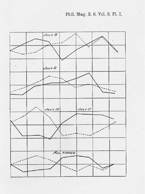
Figure 1: The Michelson-Morley fringe shifts as reported by Hicks [66]. Solid and dashed lines refer respectively to noon and evening observations.

In this framework, the fringe shift is a second-harmonic effect, i.e. periodic in the range $[0,\pi]$, whose amplitude $A_{2}$ is predicted differently by using the classical formulas or Lorentz transformations (29)

$$A^{\rm class}_{2}={{L}\over{\lambda}}{{{v}^{2}}\over{c^{2}}}~{}~{}~{}~{}~{}~{}~{}~{}~{}~{}~{}~{}~{}~{}~{}~{}~{}~{}~{}~{}~{}~{}~{}~{}~{}~{}~{}A^{\rm rel}_{2}={{L}\over{\lambda}}{{{v_{\rm obs}}^{2}}\over{c^{2}}}\sim 2({\cal N}-1)A^{\rm class}_{2}$$ (45)

Notice also that upon rotation of $\pi/2$ with respect to $\theta=\theta_{0}$ the predicted fringe shift is $2{A}_{2}$. Now, for the Michelson-Morley interferometer the whole effective optical path was about $L=11$ meters, or about $2\cdot 10^{7}$ in units of light wavelengths, so for a velocity $v\sim 30$ km/s (the Earth’s orbital velocity about the Sun, and consequently the minimum anticipated drift velocity) the expected classical 2nd-harmonic amplitude was ${A}^{\rm class}_{2}\sim 0.2$. This value can thus be used as a reference point to obtain an observable velocity, in the plane of the interferometer, from the actual measured value of $A_{2}$ through the relation

$$v_{\rm obs}\sim 30~{}\sqrt{{{A_{2}}\over{0.2}}}~{}~{}{\rm km/s}$$ (46)

Michelson and Morley performed their six observations in 1887, on July 8th, 9th, 11th and 12th, at noon and in the evening, in the basement of the Case Western University of Cleveland. Each experimental session consisted of six turns of the interferometer performed in about 36 minutes. As well summarized by Miller in 1933 [65], “The brief series of observations was sufficient to show clearly that the effect did not have the anticipated magnitude. However, and this fact must be emphasized, the indicated effect was not zero”.

The same conclusion had already been obtained by Hicks in 1902 [66]: ”..the data published by Michelson and Morley, instead of giving a null result, show distinct evidence for an effect of the kind to be expected”. Namely, there was a second-harmonic effect. But its amplitude was substantially smaller than the classical expectation (see Fig.1).

Quantitatively, the situation can be summarized in Figure 2, taken from Miller [65], where the values of the effective velocity measured in various ether-drift experiments are reported and compared with a smooth curve fitted by Miller to his own results as function of the sidereal time.

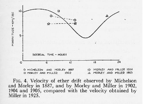
Figure 2: The magnitude of the observable velocity measured in various experiments as reported by Miller [65].

For the Michelson-Morley experiment, the average observable velocity reported by Miller is about 8.4 km/s. Comparing with the classical prediction for a velocity of 30 km/s, this means an experimental 2nd- harmonic amplitude

$$A^{\rm EXP}_{2}\sim 0.2~{}({{8.4}\over{30}})^{2}\sim 0.016$$ (47)

which is about twelve times smaller than the expected result.

Neither Hicks nor Miller reported an estimate of the error on the 2nd harmonic extracted from the Michelson-Morley data. To understand the precision of their readings, we can look at the original paper [61] where one finds the following statement : ”The readings are divisions of the screw-heads. The width of the fringes varied from 40 to 60 divisions, the mean value being near 50, so that one division means 0.02 wavelength”. Now, in their tables Michelson and Morley reported the readings with an accuracy of 1/10 of a division (example 44.7, 44.0, 43.5,..). This means that the nominal accuracy of the readings was $\pm 0.002$ wavelengths. In fact, in units of wavelengths, they reported values such as 0.862, 0.832, 0.824,.. Furthermore, this estimate of the error agrees well with Born’s book [67]. In fact, Born, when discussing the classically expected fractional fringe shift upon rotation of the apparatus by $90^{o}$, about 0.37, explicitly says: “Michelson was certain that the one-hundredth part of this displacement would still be observable” (i.e. 0.0037). Therefore, to be consistent with both the original Michelson-Morley article and Born’s quotation of Michelson’s thought, we shall adopt $\pm 0.004$ as an estimate of the error .

With this premise, the Michelson-Morley data were re-analyzed in ref.[51]. To this end, one should first follow the well defined procedure adopted in the classical experiments as described in Miller’s paper [65]. Namely, by starting from each set of seventeen entries (one every $22.5^{o}$), say $E(i)$, one has first to correct the data for the observed linear thermal drift. This is responsible for the difference $E(1)-E(17)$ between the 1st entry and the 17th entry obtained after a complete rotation of the apparatus. In this way, by adding 15/16 of the correction to the 16th entry, 14/16 to the 15th entry and so on, one obtains a set of 16 corrected entries

$$E_{\rm corr}(i)={{i-1}\over{16}}(E(1)-E(17))+E(i)$$ (48)

The fringe shifts are then defined by the differences between each of the corrected entries $E_{\rm corr}(i)$ and their average value $\langle E_{\rm corr}\rangle$ as

$${{\Delta\lambda(i)}\over{\lambda}}=E_{\rm corr}(i)-\langle E_{\rm corr}\rangle$$ (49)

The resulting data are reported in Table 1.

Table 1: The fringe shifts ${{\Delta\lambda(i)}\over{\lambda}}$ for all noon (n.) and evening (e.) sessions of the Michelson-Morley experiment.

i	July 8 (n.)	July 9 (n.)	July 11 (n.)	July 8 (e.)	July 9 (e.)	July 12 (e.)
1	$-$0.001	+0.018	+0.016	$-$0.016	+0.007	+0.036
2	+0.024	$-$0.004	$-$0.034	+0.008	$-$0.015	+0.044
3	+0.053	$-$0.004	$-$0.038	$-$0.010	+0.006	+0.047
4	+0.015	$-$0.003	$-$0.066	+0.070	+0.004	+0.027
5	$-$0.036	$-$0.031	$-$0.042	+0.041	+0.027	$-$0.002
6	$-$0.007	$-$0.020	$-$0.014	+0.055	+0.015	$-$0.012
7	+0.024	$-$0.025	+0.000	+0.057	$-$0.022	+0.007
8	+0.026	$-$0.021	+0.028	+0.029	$-$0.036	$-$0.011
9	$-$0.021	$-$0.049	+0.002	$-$0.005	$-$0.033	$-$0.028
10	$-$0.022	$-$0.032	$-$0.010	+0.023	+0.001	$-$0.064
11	$-$0.031	+0.001	$-$0.004	+0.005	$-$0.008	$-$0.091
12	$-$0.005	+0.012	+0.012	$-$0.030	$-$0.014	$-$0.057
13	$-$0.024	+0.041	+0.048	$-$0.034	$-$0.007	$-$0.038
14	$-$0.017	+0.042	+0.054	$-$0.052	+0.015	+0.040
15	$-$0.002	+0.070	+0.038	$-$0.084	+0.026	+0.059
16	+0.022	$-$0.005	+0.006	$-$0.062	+0.024	+0.043

Table 2: The amplitude of the fitted second-harmonic component $A^{\rm EXP}_{2}$ for the six experimental sessions of the Michelson-Morley experiment.

SESSION	$A^{\rm EXP}_{2}$
July 8 (noon)	$0.010\pm 0.005$
July 9 (noon)	$0.015\pm 0.005$
July 11 (noon)	$0.025\pm 0.005$
July 8 (evening)	$0.014\pm 0.005$
July 9 (evening)	$0.011\pm 0.005$
July 12 (evening)	$0.024\pm 0.005$

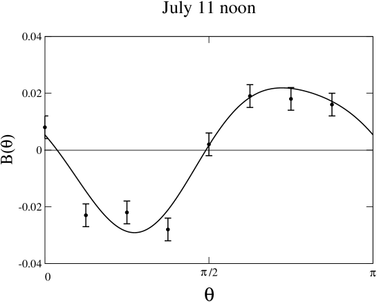
Figure 3: A fit to the even combination $B(\theta)$ Eq.(50). The second harmonic amplitude is ${A}^{\rm EXP}_{2}=0.025\pm 0.005$ and the fourth harmonic is ${A}^{\rm EXP}_{4}=0.004\pm 0.005$. The figure is taken from ref.[51]. Compare the data with the solid curve of July 11th shown in Fig.1.

With this procedure, the fringe shifts Eq.(49) are given as a periodic function, with vanishing mean, in the range $0\leq\theta\leq 2\pi$, with $\theta={{i-1}\over{16}}~{}2\pi$, so that they can be reproduced in a Fourier expansion. Notice that in the evening observations the apparatus was rotated in the opposite direction to that of noon.

One can thus extract the amplitude and the phase of the 2nd-harmonic component by fitting the even combination of fringe shifts

$$B(\theta)={{\Delta\lambda(\theta)+\Delta\lambda(\pi+\theta)}\over{2\lambda}}$$ (50)

(see Fig.3). This is essential to cancel the 1st-harmonic contribution originally pointed out by Hicks [66]. Its theoretical interpretation is in terms of the arrangements of the mirrors and, as such, this effect has to show up in the outcome of real experiments. For more details, see the discussion given by Miller, in particular Fig.30 of ref.[65], where it is shown that his observations were well consistent with Hicks’ theoretical study. The observed 1st-harmonic effect is sizeable, of comparable magnitude or even larger than the second-harmonic effect. The same conclusion was also obtained by Shankland et al. [68] in their re-analysis of Miller’s data. The 2nd-harmonic amplitudes from the six individual sessions are reported in Table 2.

Due to their reasonable statistical consistency, one can compute the mean and variance of the six determinations reported in Table 2 by obtaining $A^{\rm EXP}_{2}\sim 0.016\pm 0.006$. This value is consistent with an observable velocity

$$v_{\rm obs}\sim 8.4^{+1.5}_{-1.7}~{}~{}~{}{\rm km/s}$$ (51)

Then, by using Eq.(30), which connects the observable velocity to the projection of the kinematical velocity in the plane of the interferometer through the refractive index of the medium where light propagation takes place (in our case air where ${\cal N}\sim 1.00029$), we can deduce the average value

$$v\sim 349^{+62}_{-70}~{}{\rm km/s}$$ (52)

While the individual values of $A_{2}$ show a reasonable consistency, there are substantial changes in the apparent direction $\theta_{0}$ of the ether-drift effect in the plane of the interferometer. This is the reason for the strong cancelations obtained when fitting together all noon sessions or all evening sessions [69]. For instance, for the noon sessions, by taking into account that the azimuth is always defined up to $\pm 180^{o}$, one choice for the experimental azimuths is $357^{o}\pm 14^{o}$, $285^{o}\pm 10^{o}$ and $317^{o}\pm 8^{o}$ respectively for July 8th, 9th and 11th. For this assignment, the individual velocity vectors $v_{\rm obs}(\cos\theta_{0},-\sin\theta_{0})$ and their mean are shown in Fig.4.

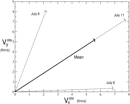
Figure 4: The observable velocities for the three noon sessions and their mean. The x-axis corresponds to $\theta_{0}=0^{o}\equiv 360^{o}$ and the y-axis to $\theta_{0}=270^{o}$. Statistical uncertainties of the various determinations are ignored. All individual directions could also be reversed by 180^o.

According to the usual interpretation, the large spread of the azimuths is taken as indication that any non-zero fringe shift is due to pure instrumental effects. However, as anticipated in Sect.2, this type of discrepancy could also indicate an unconventional form of ether-drift where there are substantial deviations from Eq.(24) and/or from the smooth trend in Eqs.(31)$-$(34). For instance, in agreement with the general structure Eq.(23), and differently from July 11 noon, which represents a very clean indication, there are sizeable 4th- harmonic contributions (here ${A}^{\rm EXP}_{4}=0.019\pm 0.005$ and ${A}^{\rm EXP}_{4}=0.008\pm 0.005$ for the noon sessions of July 8 and July 9 respectively). In any case, the observed strong variations of $\theta_{0}$ are in qualitative agreement with the analogous values reported by Miller. To this end, compare with Fig.22 of ref.[65] and in particular with the large scatter of the data taken around August 1st, as this represents the epoch of the year which is closer to the period of July when the Michelson-Morley observations were actually performed. Thus one could also conclude that individual experimental sessions indicate a definite non-zero ether-drift but the azimuth does not exhibit the smooth trend expected from the conventional picture Eqs.(31)$-$(34).

For completeness, we add that the large spread of the $\theta_{0}-$values might also reflect a particular systematic effect pointed out by Hicks [66]. As described by Miller [65], “ before beginning observations the end mirror on the telescope arm is very carefully adjusted to secure vertical fringes of suitable width. There are two adjustments of the angle of this mirror which will give fringes of the same width but which produce opposite displacements of the fringes for the same change in one of the light-paths”. Since the relevant shifts are extremely small, “…the adjustments of the mirrors can easily change from one type to the other on consecutive days. It follows that averaging the results of different days in the usual manner is not allowable unless the types are all the same. If this is not attended to, the average displacement may be expected to come out zero $-$ at least if a large number are averaged” [66]. Therefore averaging the fringe shifts from various sessions represents a delicate issue and can introduce uncontrolled errors. Clearly, this relative sign does not affect the values of $A_{2}$ and this is why averaging the 2nd-harmonic amplitudes is a safer procedure. However, it can introduce spurious changes in the apparent direction $\theta_{0}$ of the ether-drift. In fact, an overall change of sign of the fringe shifts at all $\theta-$values is equivalent to replacing $\theta_{0}\to\theta_{0}\pm\pi/2$. As a matter of fact, Hicks concluded that the fringes of July 8th were of different type from those of the remaining days. Thus for his averages (in our Fig.1) “the values of the ordinates are one-third of July 9 + July 11 $-$ July 8 and one-third of July 9 + July 12 $-$ July 8” [66] for noon and evening sessions respectively. If this were true, one choice for the azimuth of July 8th could now be $\theta^{\rm EXP}_{0}=267^{o}\pm 14^{o}$. This would orient the arrow of July 8th in Fig.4 in the direction of the y$-$axis and change the average azimuth from $\langle\theta^{\rm EXP}_{0}\rangle\sim 317^{o}$ to $\langle\theta^{\rm EXP}_{0}\rangle\sim 290^{o}$. We’ll return to this particular aspect in our Appendix II.

Let us finally compare with the interpretation that Michelson and Morley gave of their data. They start from the observation that ”…the displacement to be expected was 0.4 fringe” while ”…the actual displacement was certainly less than the twentieth part of this”. In this way, since the displacement is proportional to the square of the velocity, ”…the relative velocity of the earth and the ether is… certainly less than one-fourth of the orbital earth’s velocity”. The straightforward translation of this upper bound is $v_{\rm obs}<$ 7.5 km/s. However, this estimate is likely affected by a theoretical uncertainty. In fact, in their Fig.6, Michelson and Morley reported their measured fringe shifts together with the plot of a theoretical second-harmonic component. In doing so, they plotted a wave of amplitude $A_{2}=0.05$, that they interpret as one-eight of the theoretical displacement expected on the base of classical physics, thus implicitly assuming $A^{\rm class}_{2}$=0.4. As discussed above, the amplitude of the classically expected second-harmonic component is not 0.4 but is just one-half of that, i.e. 0.2. Therefore, their experimental upper bound $A^{\rm exp}_{2}<{{0.4}\over{20}}=$0.02 is actually equivalent to $v_{\rm obs}<$ 9.5 km/s. If we now consider that their estimates were obtained after superimposing the fringe shifts obtained from various sessions (where the overall effect is reduced, see our Fig.1), we deduce a substantial agreement with our result Eq. (51).

4. Morley-Miller

After the original 1887 experiment, there was much interest in the Michelson-Morley result that, being too small to meet any classical prediction, was apparently contradicting two cornerstones of physics: Galilei’s transformations and/or the existence of the ether. For this reason, one of the most influential physicists of the time, Lord Kelvin, after his conference at the 1900 Paris Expo, induced Morley and his young collaborator Dayton Miller to design a new interferometer (where the effective optical path was increased up to 32 meters) to improve the accuracy of the measurement over the 1887 result.

It must be emphasized that Morley and Miller [70], in their observations of 1905, superimposed the data of the morning with those of the evening. As explained by Miller [63], the two physicists were assuming that the ether drift had to be obtained by combining the motion of the solar system relative to nearby stars, i.e. toward the constellation of Hercules with a velocity of about 19 km/s, with the annual orbital motion (“We now computed the direction and the velocity of the motion of the centre of the apparatus by compounding the annual motion in the orbit of the earth with the motion of the solar system toward a certain point in the heavens…There are two hours in each day when the motion is in the desired plane of the interferometer” [70]). The observations at the two times (about 11:30 a.m. and 9:00 p.m.) were, therefore, combined in such a way that the presumed azimuth for the morning observations coincided with that for the evening (“The direction of the motion with reference to a fixed line on the floor of the room being computed for the two hours, we were able to superimpose those observations which coincided with the line of drift for the two hours of observation” [70]). However, the observations for the two times of the day gave results having nearly opposite phases. When these were combined, the result was nearly zero. For this reason, the value then reported of an observable velocity of 3.5 km/s is incorrect and does not correspond to the actual results of the basic observations. The error was later understood and corrected by Miller who found that the two sets of data were each indicating an effective velocity of about 7.5 km/s (see Figure 11 of Miller’s paper [65]). For this reason, the correct average observable velocities for the entire period 1902-1905 are those shown in our Figure 2 between 7 and 10 km/s or

$$v_{\rm obs}\sim(8.5\pm 1.5)~{}{\rm km/s}$$ (53)

By using Eq.(30), we then deduce the average value

$$v\sim(353\pm 62)~{}{\rm km/s}$$ (54)

5. Kennedy-Illingworth

An interesting development was proposed by Kennedy in 1926. As summarized in his contribution to the previously mentioned Conference on the Michelson-Morley experiment [63], his small optical system was enclosed in an effectively insulated, sealed metal case containing helium at atmospheric pressure. Because of its small size, ”…circulation and variation in density of the gas in the light paths were nearly eliminated. Furthermore, since the value of ${\cal N}-1$ is only about 1/10 that for the air at the same pressure, the disturbing changes in density of the gas correspond to those in air to only 1/10 of the atmospheric pressure”. The essential ingredient of Kennedy’s apparatus consisted in the introduction of a small step, 1/20 of wavelength thick, in one of the total reflecting mirrors of the interferometer allowing, in principle, for an ultimate fringe shift accuracy $1\cdot 10^{-4}$. To take full advantage of this possibility, Kennedy should have disposed of perfect mirrors and of a suitable (hotter) source of light. In the original version of the experiment, these refinements were not implemented giving an actual fringe shift accuracy of $2\cdot 10^{-3}$. In these conditions, as Kennedy explicitly says[63], ”…the velocity of 10 km/s found by Prof. Miller would produce a fringe shift corresponding to $8\cdot 10^{-3}$”, four times larger than the experimental resolution. Since the effect is quadratic in the velocity, Kennedy’s result, fringe shifts $<2\cdot 10^{-3}$, can then be summarized as

$$v_{\rm obs}<5~{}{\rm km/s}$$ (55)

By using Eq.(30), for helium at atmospheric pressure where ${\cal N}\sim 1.000035$, this bound amounts to restrict the kinematical value by $v<$ 600 km/s.

Table 3: The infra-session averages $\langle D_{A}\rangle$ and $\langle D_{B}\rangle$ obtained from the 10 sets of rotations in each of the 32 sessions of Illingworth’s experiment. These values have been obtained from the weights of Illingworth’s Table III by applying the conversion factor 0.002.

5 A.M.	5 A.M.	11 A.M.	11 A.M.	5 P.M.	5 P.M.	11 P.M.	11 P.M.
$\rm\langle D_{A}\rangle$	$\rm\langle D_{B}\rangle$	$\rm\langle D_{A}\rangle$	$\rm\langle D_{B}\rangle$	$\rm\langle D_{A}\rangle$	$\rm\langle D_{B}\rangle$	$\rm\langle D_{A}\rangle$	$\rm\langle D_{B}\rangle$
$+0.00024$	$-0.00066$	$+0.00070$	$-0.00022$	$+0.00024$	$+0.00044$	$-0.00010$	$+0.00024$
$+0.00114$	$+0.00024$	$-0.00042$	$-0.00036$	$-0.00056$	$-0.00046$	$+0.00018$	$+0.00018$
$+0.00000$	$+0.00000$	$-0.00006$	$-0.00052$	$-0.00144$	$-0.00080$	$-0.00126$	$-0.00006$
$+0.00020$	$-0.00044$	$-0.00030$	$+0.00012$	$-0.00016$	$+0.00004$	$-0.00044$	$-0.00026$
$+0.00064$	$+0.00000$	$-0.00022$	$+0.00038$	$+0.00018$	$+0.00016$	$+0.00000$	$+0.00024$
$-0.00002$	$-0.00010$	$+0.00048$	$+0.00020$	$+0.00030$	$+0.00030$	$-0.00040$	$-0.00004$
		$-0.00014$	$-0.00006$	$+0.00030$	$+0.00014$
		$-0.00006$	$+0.00004$	$+0.00036$	$-0.00036$
		$-0.00006$	$+0.00016$	$+0.00006$	$-0.00006$
		$+0.00000$	$+0.00024$	$-0.00010$	$+0.00010$

Kennedy’s apparatus was further refined by Illingworth in 1927 [71]. Besides improving the quality of the mirrors and of the source, Illingworth’s data taking was also designed to reduce the presence of steady thermal drift and of odd harmonics. Looking at Illingworth’s paper, one finds that his refinements reached indeed the nominal ${\cal O}(10^{-4})$ accuracy mentioned by Kennedy, namely about 1/1500 of wavelength for the individual readings and $(1\div 2)\cdot 10^{-4}$ at the level of average values.

Let us now analyze Illingworth’s results. He performed four series of observations in the first ten days of July 1927. These consisted of 32 experimental sessions, conducted daily at 5 A.M. (6), 11 A.M. (10), 5 P.M. (10) and 11 P.M.(6), in which he was measuring the fringe displacement caused by a rotation through a right angle of the apparatus. To take into account $90^{o}$ rotations let us first re-write Eq.(29) as

$${{\Delta\lambda(\theta)}\over{\lambda}}=A_{2}\cos 2(\theta-\theta_{0})$$ (56)

Therefore Illingworth, in his first set (set A) of 10 rotations, North, East, South, West and back to North, was actually measuring $D_{A}\equiv 2A_{2}\cos 2\theta_{0}$. In a second set (set B), North-East, North-West, South-West, South-East and back to North-East, performed immediately after the set A, he was then measuring $D_{B}\equiv 2A_{2}\sin 2\theta_{0}$. Notice that both $D_{A}$ and $D_{B}$ differ from the positive-definite quantity $D\equiv 2A_{2}$ that should be inserted in Illingworth’s numerical relation for his apparatus $v_{\rm obs}=112\sqrt{D}$. Therefore, the reported values for the two velocities $v_{A}=112\sqrt{|D_{A}|}$ and $v_{B}=112\sqrt{|D_{B}|}$ should only be taken as lower bounds for the true $v_{\rm obs}$. The mean values $\langle D_{A}\rangle$ and $\langle D_{B}\rangle$ obtained from the 10 sets of rotations in the 32 individual sessions can be obtained from Illingworth’s Table III and, for the convenience of the reader, are reported in our Table 3.

From Table 3, one finds that the quantity $\sqrt{\langle D_{A}\rangle^{2}+\langle D_{B}\rangle^{2}}$ has a mean value of about 0.00045, which corresponds to $v_{\rm obs}\sim 2.4$ km/s. Thus, by using Eq.(30) for helium at atmospheric pressure, we would tentatively deduce an average value $v\sim 284$ km/s.

However, this is only a very partial view. To go deeper into Illingworth’s experiment we have to consider his basic measurements, i.e. the individual turns of his interferometer. In this case, the only known basic set of data reported by Illingworth is set A of July 9th, 11 A.M. This set has been re-analyzed by Múnera [72] and his values for the fringe shifts are reported in our Table 4.

Table 4: Illingworth’s set A of July 9th, 11 A.M. as re-analyzed by Múnera [72].

Rotation	$\rm D_{A}$	$\rm|D_{A}|$	$\rm v_{A}$[km/s]
1	$-0.00100$	$+0.00100$	3.54
2	$+0.00066$	$+0.00066$	2.89
3	$-0.00066$	$+0.00066$	2.89
4	$-0.00066$	$+0.00066$	2.89
5	$-0.00166$	$+0.00166$	4.57
6	$+0.00234$	$+0.00234$	5.41
7	$+0.00100$	$+0.00100$	3.54
8	$+0.00034$	$+0.00034$	2.04
9	$+0.00000$	$+0.00000$	0.00
10	$-0.00100$	$+0.00100$	3.54

As one can see, the fringe shifts are not small and correspond to an observable velocity in the range 2-5 km/s. However, their sign seems to change randomly. Therefore, if one attempts to extract the observable velocity from the mean of the 10 determinations, $\langle D_{A}\rangle\sim-0.00006$, the resulting value 0.9 km/s is much smaller than all individual determinations. The basis of Múnera’s analysis was instead to estimate $v_{\rm obs}$ from $\langle|D_{A}|\rangle$, from which he obtained an average velocity $v_{\rm obs}=3.13\pm 1.04$ km/s.

Now, the standard interpretation of such apparently random changes of sign is in terms of typical instrumental effects and the standard method for eliminating these is the original averaging procedure as employed by Illingworth. But we will now show that they could also indicate an unconventional form of stochastic drift, of the type already mentioned in the previous sections, and in which Múnera’s re-estimate has a definite significance. To this end, we shall first use the relations

$$D_{A}(t)=4C(t)~{}~{}~{}~{}~{}~{}~{}~{}~{}~{}~{}~{}~{}~{}~{}~{}~{}~{}~{}~{}~{}D_{B}(t)=4S(t)$$ (57)

where the two functions $C(t)$ and $S(t)$ have been introduced in Eqs.(36) and (44). Thus Eqs.(57) can be re-written as

$$D_{A}(t)={{8L({\cal N}-1)}\over{\lambda}}~{}{{v^{2}_{x}(t)-v^{2}_{y}(t)}\over{2c^{2}}}~{}~{}~{}~{}~{}~{}~{}~{}~{}~{}~{}~{}~{}~{}D_{B}(t)={{8L({\cal N}-1)}\over{\lambda}}~{}{{v_{x}(t)~{}v_{y}(t)}\over{c^{2}}}$$ (58)

where $v_{x}(t)=v(t)\cos\theta_{0}(t)$ and $v_{y}(t)=v(t)\sin\theta_{0}(t)$. In this way, by using the numerical relation for Illingworth’s experiment ${{L}\over{\lambda}}~{}{{(30{\rm km/s})^{2}}\over{c^{2}}}\sim 0.035$ and the value of the helium refractive index, we obtain

$$D_{A}(t)\sim{{v^{2}_{x}(t)-v^{2}_{y}(t)}\over{\rm 2\cdot(300~{}km/s)^{2}}}\cdot 10^{-3}~{}~{}~{}~{}~{}~{}~{}~{}~{}~{}~{}~{}~{}~{}D_{B}(t)\sim{{v_{x}(t)~{}v_{y}(t)}\over{\rm(300~{}km/s)^{2}}}\cdot 10^{-3}~{}$$ (59)

The required random ingredient can then be introduced by characterizing the two velocity components $v_{x}(t)$ and $v_{y}(t)$ as turbulent fluctuations. To this end, there can be several ways. Here we shall restrict to the simplest choice of a turbulence which, at small scales, appears statistically isotropic and homogeneous . This represents a zeroth-order approximation which is motivated by the substantial reading error of the Illingworth measurements (it turns out to be comparable to the effects of turbulence). However, it is a useful example to illustrate basic phenomenological features associated with an underlying stochastic vacuum. To explore the resulting temporal pattern of the data, we have followed refs.[74, 75] where velocity flows, in statistically isotropic and homogeneous 3-dimensional turbulence, are generated by unsteady random Fourier series. The perspective is that of an observer moving in the turbulent fluid who wants to simulate the two components of the velocity in his x-y plane at a given fixed location in his laboratory. This leads to the general expressions

$$v_{x}(t)=\sum^{\infty}_{n=1}\left[x_{n}(1)\cos\omega_{n}t+x_{n}(2)\sin\omega_{n}t\right]$$ (60)

$$v_{y}(t)=\sum^{\infty}_{n=1}\left[y_{n}(1)\cos\omega_{n}t+y_{n}(2)\sin\omega_{n}t\right]$$ (61)

where $\omega_{n}=2n\pi/T$, T being a time scale which represents a common period of all stochastic components. We have adopted the typical value $T=T_{\rm day}$= 24 hours. However, we have also checked with a few runs that the statistical distributions of the various quantities do not change substantially by varying $T$ in the rather wide range $0.1~{}T_{\rm day}\leq T\leq 10~{}T_{\rm day}$.

The coefficients $x_{n}(i=1,2)$ and $y_{n}(i=1,2)$ are random variables with zero mean. They have the physical dimension of a velocity and we shall denote by $[-\tilde{v},\tilde{v}]$ the common interval for these four parameters. In terms of $\tilde{v}$ the statistical average of the quadratic values can be expressed as

$$\langle x^{2}_{n}(i=1,2)\rangle_{\rm stat}=\langle y^{2}_{n}(i=1,2)\rangle_{\rm stat}={{{\tilde{v}}^{2}}\over{3~{}n^{2\eta}}}$$ (62)

for the uniform probability model (within the interval $[-\tilde{v},\tilde{v}]$) which we have chosen for our simulations. Finally, the exponent $\eta$ controls the power spectrum of the fluctuating components. For the simulations, between the two values $\eta=5/6$ and $\eta=1$ reported in ref.[75], we have chosen $\eta=1$ which corresponds to the point of view of an observer moving in the fluid.

Thus, within this simple model for $D_{A}(t)$ and $D_{B}(t)$, $\tilde{v}$ is the only parameter whose numerical value could reflect the properties of a large-scale motion, for instance of the Earth’s motion with respect to the Cosmic Microwave Background (CMB). For this reason, here, we have adopted the fixed value $\tilde{v}=V_{\rm CMB}=$ 370 km/s.

Figure 5: A simulation of $\rm D_{A}(t)$ and $\rm D_{B}(t)$, in units $10^{-3}$ and every 30 seconds, from typical sequences of 1200 seconds. The average values are $\langle D_{A}\rangle=0.00028$ and $\langle D_{B}\rangle=0.00011$. The velocity parameter is $\tilde{v}=V_{\rm CMB}=$ 370 km/s.

With these premises, our results can be illustrated by first considering the basic set of 10 complete rotations of the apparatus during which Illingworth’s fringe shifts (produced by $90^{o}$ rotations) were recorded every 30 seconds. Therefore, this type of simulations consists in generating 40 values during a total time of 1200 seconds. As an illustration, two typical sequences of $\rm D_{A}(t)$ and $\rm D_{B}(t)$, in units $10^{-3}$, are shown in Fig.5.

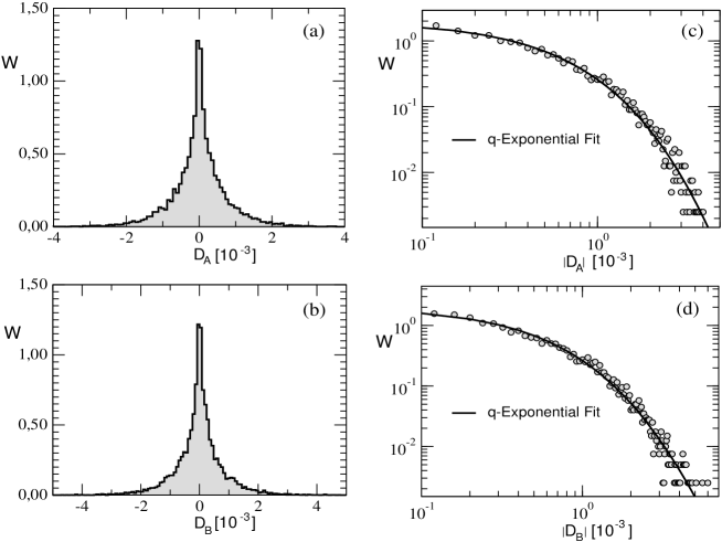
Figure 6: We show, see (a) and (b), the histograms $W$ obtained from a simulation for $\rm D_{A}=D_{A}(t)$ and $\rm D_{B}=D_{B}(t)$. The vertical normalization is to a unit area. The mean values are $\rm\langle D_{A}\rangle=0.75\cdot 10^{-5}$, $\rm\langle D_{B}\rangle=-1.1\cdot 10^{-5}$ and the standard deviations $\rm\sigma(D_{A})=0.75\cdot 10^{-3}$, $\rm\sigma(D_{B})=0.83\cdot 10^{-3}$. We also show, see (c) and (d), the corresponding plots in logarithmic scale and the fits with Eq.(63). The parameters of the fit are q=1.07, a=2 and b=2.2 for $\rm D_{A}$ and q=1.12, a=2 and b=2.3 for $\rm D_{B}$. The total statistics correspond to 10.000 values generated at steps of 30 seconds. The velocity parameter is $\tilde{v}=V_{\rm CMB}=$ 370 km/s.

As one can see, the magnitude ${\cal O}(10^{-3})$ and the random nature of the instantaneous values is completely consistent with the entries of Table 4. Also the resulting infra-session averages $\langle D_{A}\rangle=0.00028$ and $\langle D_{B}\rangle=0.00011$ are completely consistent with the typical entries of Table 3.

To obtain further insight, we have then performed extensive simulations for large sequences of measurements. The histograms of a set of 10000 determinations of $D_{A}(t)$ and $D_{B}(t)$ (again generated every 30 seconds) are reported in panels (a) and (b) of Fig.6.

Notice that these distributions are clearly “fat-tailed” and very different from a Gaussian shape. This kind of behavior is characteristic of probability distributions for instantaneous data in turbulent flows (see e.g. [76, 77]). To better appreciate the deviation from Gaussian behavior, in panels (c) and (d) we plot the same data in a log$-$log scale. The resulting distributions are well fitted by the so-called $q-$exponential function [78]

$$f_{q}(x)=a(1-(1-q)xb)^{1/(1-q)}$$ (63)

with entropic index $q\sim 1.1$. For such large samples of data, the statistical averages $\langle D_{A}\rangle$ and $\langle D_{B}\rangle$ are vanishingly small in units of the typical instantaneous values ${\cal O}(10^{-3})$ and any non-zero average has to be considered as statistical fluctuation. On the other hand, the standard deviations $\sigma(D_{A})$ and $\sigma(D_{B})$ have definite non-zero values which reflect the magnitude of the scale parameter $\tilde{v}$. By keeping $\tilde{v}$ fixed at 370 km/s, we have found

$$\sigma(D_{A})\sim(0.74\pm 0.05)\cdot 10^{-3}~{}~{}~{}~{}~{}~{}~{}~{}~{}~{}~{}~{}~{}~{}~{}~{}~{}~{}\sigma(D_{B})\sim(0.83\pm 0.06)\cdot 10^{-3}$$ (64)

whose uncertainties reflect the observed variations due to the truncation of the Fourier modes in Eqs.(60), (61) and to the dependence on the random sequence. Taking this calculation into account gives a mean spread slightly less, about $0.65\cdot 10^{-3}$, for the effect of stochastic drift in Illingworth’s measurements. This is comparable to the uncertainty of the individual readings which, in the best case, was of 1/1500 wavelengths, i.e. $\pm 0.7\cdot 10^{-3}$. By combining in quadrature the two uncertainties, one gets a good agreement with our Table 4 where the variance of the mean is about $\pm 1\cdot 10^{-3}$. Finally, the simulation is also useful to get indications on the expected value of the observable velocity. In fact, with vanishingly small values of $\langle D_{A}\rangle$ and $\langle D_{B}\rangle$ one gets $\langle D^{2}_{A}\rangle\sim\sigma^{2}(D_{A})$ and $\langle D^{2}_{B}\rangle\sim\sigma^{2}(D_{B})$. Therefore one obtains the following two average estimates of $v_{\rm obs}$

$$v_{\rm obs}\sim 112\sqrt{\sigma(D_{A})}\sim 3.05~{}{\rm km/s}~{}~{}~{}~{}~{}~{}~{}~{}~{}~{}~{}~{}~{}~{}~{}~{}~{}~{}~{}v_{\rm obs}\sim 112\sqrt{\sigma(D_{B})}\sim 3.23~{}{\rm km/s}$$ (65)

with a mean value of 3.14 km/s which is very close to Múnera’s determination $v_{\rm obs}=3.13\pm 1.04$ km/s.

We emphasize that one could further improve the stochastic model by introducing time modulations and/or slight deviations from isotropy. For instance, $\tilde{v}$ could become a function of time $\tilde{v}=\tilde{v}(t)$. By still retaining statistical isotropy, this could be used to simulate the possible modulations of the projection of the Earth’s velocity in the plane of the interferometer. Or, one could fix a range, say $[-\tilde{v}_{x},\tilde{v}_{x}]$, for the two random parameters $x_{n}(1)$ and $x_{n}(2)$, which is different from the range $[-\tilde{v}_{y},\tilde{v}_{y}]$ for the other two parameters $y_{n}(1)$ and $y_{n}(2)$. Finally, $\tilde{v}_{x}$ and $\tilde{v}_{y}$ could also become given functions of time, for instance $\tilde{v}_{x}(t)\equiv\tilde{v}(t)\cos\tilde{\theta}_{0}(t)$ $\tilde{v}_{y}(t)\equiv\tilde{v}(t)\sin\tilde{\theta}_{0}(t)$, $\tilde{v}(t)$ and $\tilde{\theta}_{0}(t)$ being defined in Eqs. (31)$-$(34). We shall discuss this other alternative later on, in connection with the much more accurate Joos 1930 experiment.

In any case, by accepting this type of picture of the ether-drift, it is clear that further reduction of the data by performing inter-session averages ($\langle\langle...\rangle\rangle$) among the various sessions, can wash out completely the physical information contained in the original observations. In Table 5, we report the final inter-session averages $\langle\langle D_{A}\rangle\rangle$ and $\langle\langle D_{B}\rangle\rangle$ obtained by Illingworth for the various observation times.

Table 5: Illingworth’s final inter-session averages.

Observations	$\langle\langle D_{A}\rangle\rangle$	$\langle\langle D_{B}\rangle\rangle$
5 A.M.	$+0.00036\pm 0.00012$	$-0.00016\pm 0.00009$
11 A.M.	$-0.00001\pm 0.00007$	$-0.00000\pm 0.00006$
5 P.M.	$-0.00008\pm 0.00012$	$-0.00005\pm 0.00008$
11 P.M.	$-0.00034\pm 0.00014$	$+0.00005\pm 0.00006$

Nevertheless, in spite of the strong cancelations expected from the averaging reduction process mentioned above, some non-zero value is still surviving. Therefore, regardless of our simulations, one could draw the following conclusions. Traditionally, from these final averages for $\langle\langle D_{A}\rangle\rangle$ at 5 A.M. and at 11 P.M. one has been deducing the values $v_{A}\sim 2.12$ km/s and $v_{A}\sim 2.07$ km/s respectively. Therefore, from these two estimates of $v_{A}$ that, as anticipated, represent lower bounds for $v_{\rm obs}$, it follows that there were values of $v_{\rm obs}$ which clearly had to be larger than both. For this reason, this 2.1 km/s velocity value reported by Illingworth, rather than being interpreted as an upper bound could also be interpreted as a lower bound placed by his experiment. In this way, by combining with the previous Kennedy’s upper bound $v_{\rm obs}<5$ km/s, one would deduce that these two experiments, where light was propagating in helium at atmospheric pressure, give a range for the observable velocity

$${\rm(Kennedy+Illingworth)}\hskip 80.0pt2~{}{\rm km/s}\lesssim v_{\rm obs}<5~{}{\rm km/s}\hskip 90.0pt$$ (66)

in complete agreement with Múnera’s determination

$$v_{\rm obs}=3.1\pm 1.0~{}{\rm km/s}$$ (67)

From this last estimate, by using Eq.(30) and taking into account that for helium at atmospheric pressure the refractive index is ${\cal N}\sim 1.000035$, one obtains a kinematical velocity

$$v\sim(370\pm 120)~{}{\rm km/s}$$ (68)

consistently with the velocity values Eqs.(52) and (54) from the Michelson-Morley and Morley-Miller experiments.

6. Miller

Múnera’s analysis [72] is also interesting because he applied the same method used for Illingworth’s observations to the only known Miller set of data explicitly reported in the literature. In this case, his value $v_{\rm obs}=8.2\pm 1.4$ km/s, after correcting with Eq.(30), confirms the estimate $v\sim 350$ km/s for the average velocity in the plane of the interferometer.

This close agreement with the Michelson-Morley value 8.4 km/s is also confirmed by the critical re-analysis of Shankland et al. [68]. Differently from the original Michelson-Morley experiment, Miller’s data were taken over the entire day and in four epochs of the year. However, after the critical re-analysis of the original raw data performed by the Shankland team, there is now an independent estimate of the average determinations $A^{\rm EXP}_{2}$ for the four epochs. Their values 0.042, 0.049, 0.038 and 0.045, respectively for April 1925, July 1925, September 1925 and February 1926 (see page 170 of ref.[68]) are so well statistically consistent that one can easily average them. The overall determination from Table III of [68]

$$A^{\rm EXP}_{2}=0.044\pm 0.022$$ (69)

when compared with the equivalent classical prediction for Miller’s interferometer $A^{\rm class}_{2}={{L}\over{\lambda}}{{(30{\rm km/s})^{2}}\over{c^{2}}}\sim 0.56$ corresponds to an average observable velocity

$$v_{\rm obs}=8.4^{+1.9}_{-2.5}~{}{\rm km/s}$$ (70)

and, by using Eq.(30), to a true kinematical value

$$v=349^{+79}_{-104}~{}{\rm km/s}$$ (71)

We are aware that our conclusion goes against the widely spread belief, originating precisely from the paper of Shankland et al. ref.[68], that Miller’s results might actually have been due to statistical fluctuation and/or local temperature conditions. To a closer look, however, the arguments of Shankland et al. are not so solid as they appear when reading the Abstract of their paper . In fact, within the paper these authors say that “…there can be little doubt that statistical fluctuations alone cannot account for the periodic fringe shifts observed by Miller” (see page 171 of ref.[68]). Further, although “…there is obviously considerable scatter in the data at each azimuth position,…the average values…show a marked second harmonic effect” (see page 171 of ref.[68]). In any case, interpreting the observed effects on the basis of the local temperature conditions is certainly not the only explanation since “…we must admit that a direct and general quantitative correlation between amplitude and phase of the observed second harmonic on the one hand and the thermal conditions in the observation hut on the other hand could not be established” (see page 175 of ref.[68]).

Table 6: The symmetric combination of fringe shifts $B(\theta)={{\Delta\lambda(\theta)+\Delta\lambda(\pi+\theta)}\over{2\lambda}}$ at the various values of $\theta$ for the set of 20 turns of the interferometer reported in Fig.8 of ref.[65]. For our global fit, following ref.[68], the nominal accuracy of each entry has been fixed to $\pm 0.050$.

Turn	$0^{o}$	$22.5^{o}$	$45^{o}$	$67.5^{o}$	$90^{o}$	$112.5^{o}$	$135^{o}$	$157.5^{o}$
1	+0.091	+0.159	+0.028	+0.047	$-$0.034	$-$0.116	$-$0.147	$-$0.028
2	$-$0.025	+0.063	+0.050	+0.088	$-$0.075	$-$0.038	+0.000	$-$0.063
3	+0.022	+0.103	+0.084	+0.016	$-$0.053	$-$0.072	$-$0.091	$-$0.009
4	+0.034	$-$0.009	$-$0.053	$-$0.047	$-$0.041	+0.016	+0.022	+0.078
5	+0.169	+0.081	+0.044	$-$0.044	$-$0.081	$-$0.169	$-$0.056	+0.056
6	$-$0.025	+0.025	+0.025	+0.025	+0.025	$-$0.025	$-$0.025	$-$0.025
7	+0.081	+0.094	+0.056	+0.069	$-$0.119	$-$0.106	$-$0.094	+0.019
8	+0.066	+0.072	$-$0.022	$-$0.066	$-$0.059	$-$0.003	+0.003	+0.009
9	+0.041	+0.084	+0.078	+0.022	$-$0.134	$-$0.141	+0.003	+0.047
10	+0.016	+0.072	+0.078	$-$0.016	$-$0.009	$-$0.003	$-$0.047	$-$0.091
11	+0.009	+0.053	+0.097	$-$0.009	$-$0.116	$-$0.072	+0.022	+0.016
12	+0.022	+0.016	+0.059	+0.003	$-$0.053	$-$0.009	$-$0.016	$-$0.022
13	+0.000	+0.063	+0.025	+0.038	+0.050	$-$0.038	$-$0.075	$-$0.063
14	$-$0.034	+0.047	+0.078	+0.009	$-$0.009	$-$0.028	$-$0.047	$-$0.016
15	+0.113	+0.125	+0.138	+0.000	$-$0.088	$-$0.125	$-$0.113	$-$0.050
16	+0.025	+0.050	+0.025	+0.050	$-$0.025	$-$0.050	$-$0.025	$-$0.050
17	+0.000	$-$0.012	$-$0.025	+0.063	+0.000	$-$0.012	$-$0.025	+0.013
18	+0.044	+0.050	+0.019	$-$0.019	$-$0.056	$-$0.044	$-$0.031	+0.031
19	+0.053	+0.059	+0.016	$-$0.028	$-$0.022	$-$0.066	$-$0.009	$-$0.003
20	+0.059	+0.041	+0.122	+0.003	$-$0.066	$-$0.084	$-$0.053	$-$0.022

Most surprisingly, however, Shankland et al. seem not to realize that Miller’s average value $A^{\rm EXP}_{2}\sim 0.044$, obtained after their own re-analysis of his observations at Mt.Wilson, when compared with the reference classical value $A^{\rm class}_{2}=0.56$ for his apparatus, was giving the same observable velocity $v_{\rm obs}\sim 8.4$ km/s obtained from Miller’s re-analysis of the Michelson-Morley experiment in Cleveland. Conceivably, their emphasis on the role of temperature effects would have been re-considered had they realized the perfect identity of two determinations obtained in completely different experimental conditions. In this sense, an interpretation in terms of a temperature gradient is only acceptable provided this gradient represents a non-local effect, as in our model of the ether drift from a fundamental vacuum energy-momentum flow.

Another criticism of Miller’s work was recently presented by Roberts [80]. This author, using the set of data reported in Fig.8 of ref.[65], raises several objections to the validity of Miller’s observations. The two main objections concern i) the subtraction of the steady thermal drift, which was approximated by Miller as a pure linear effect, and ii) the statistical significance of the measurements. Concerning remark i), Roberts reports in his Fig.3 a broken line that reproduces the expected linear trend. He also reports some chosen points (differing from the corners of the broken line by 180 degrees) that, due to the 2nd-harmonic nature of the ether-drift effect, should lie on the line. However, this expectation ignores that, as already pointed out for the Michelson-Morley experiment, real measurements contains large first-harmonic effects. These only cancel when taking symmetric combinations of data at the various angles $\theta$ and $\pi+\theta$. As a matter of fact, the autocorrelative methods and further tests applied by the Shankland team over all of Miller’s data confirmed the linear drift approximation as remarkably good (see their footnote 21 on page 177 of [68]).

Concerning remark ii), according to Roberts, the experimental uncertainties are so large that the observed 2nd-harmonic effect has no statistical significance. To check this point we have re-computed ourselves the fringe shifts for the set of 20 turns of the interferometers (reported in Fig.8 of ref.[65]) considered by Roberts, by following the same procedure explained in Sect.3. The resulting symmetric combinations of fringe shifts

$$B(\theta)={{\Delta\lambda(\theta)+\Delta\lambda(\pi+\theta)}\over{2\lambda}}$$ (72)

are reported in our Table 6.

We have then fitted these data by including both 2nd and 4th harmonic terms. Notice that, differently from Roberts’ analysis, we do not perform any averaging of data obtained from different turns of the interferometer. For our global fit, to estimate the accuracy of the various determinations, we have followed ref.[68] and adopted a nominal uncertainty $\pm 0.050$ for each entry of Table 6. From the fit, where the 4th harmonic is completely consistent with the background ($A^{\rm EXP}_{4}=0.004\pm 0.012$), we have obtained a chi-square of 130 for $157$ degrees of freedom and the following values

$$A^{\rm EXP}_{2}=0.061\pm 0.012~{}~{}~{}~{}~{}~{}~{}~{}~{}~{}~{}~{}~{}~{}~{}~{}~{}~{}~{}~{}~{}~{}~{}~{}\theta^{\rm EXP}_{0}=24^{o}\pm 7^{o}$$ (73)

Here errors correspond to the overall boundary $\Delta\chi^{2}=+3.67$, as appropriate for a 70$\%$ C. L. in a 3-parameter fit [81]. Notice that, even though the fitted $A_{2}$ Eq.(73) is only 20$\%$ larger than the nominal accuracy $\pm 0.050$ of each entry, the data are distributed in such a way to produce a $5\sigma$ evidence for a non-zero 2nd harmonic.

As for Illingworth’s experiment, we have also analyzed the results obtained from the individual turns of the interferometer. To this end, we report in Figs. 7 and 8 the plots of the azimuth and of the 2nd harmonic for the 20 rotations.

Figure 7: The azimuth (in degrees) for the 20 individual turns of the interferometer reported in Table 6. The average uncertainty of each determination is about $\pm 20^{o}$. The band between the two horizontal lines corresponds to the global fit $\theta_{0}=24^{o}\pm 7^{o}$. Each individual value could also be reversed by 180 degrees.

Figure 8: The 2nd-harmonic amplitude for the 20 individual turns of the interferometer reported in Table 6. The average uncertainty of each determination is about $\pm 0.030$. The band between the two horizontal lines corresponds to the global fit $A_{2}=0.061\pm 0.012$. Within their errors, these individual values correspond to an observable velocity in the range 4$\div$14 km/s.

To conclude our analysis of Miller’s experiment, we want to mention that other objections to the overall consistency of his solution for the Earth’s cosmic motion [65] were raised by von Laue [82] and Thirring [83]. Their argument, which concerns the observed displacement of the maximum of the fringe pattern averaged over all sidereal times, was also re-proposed by Shankland et al. [68] and amounts to the following.

By assuming relations (31)$-$(43) and denoting by $\langle...\rangle$ the daily average of any given quantity, one finds, at any angle $\theta$, the daily averaged fringe shift

$$\langle{{\Delta\lambda(\theta)}\over{\lambda}}\rangle=2\langle\tilde{C}(t)\rangle\cos 2\theta$$ (74)

since $\langle\tilde{S}(t)\rangle=0$ with

$$\langle\tilde{C}(t)\rangle=-{{L({\cal N}-1)}\over{\lambda}}{{V^{2}}\over{c^{2}}}~{}{{1}\over{4}}(3\cos 2\gamma-1)\cos^{2}\phi$$ (75)

The result can then be cast into the form [68]

$$\langle{{\Delta\lambda(\theta)}\over{\lambda}}\rangle=V^{2}F(\gamma,\phi)\cos 2\theta$$ (76)

Therefore, since the latitude $\phi$ is a constant and the angular declination $\gamma$ is fixed at any specific epoch, the daily averaged fringe shifts should all have a common maximum at the value $\theta=0$. Only the amplitude can be different at different epochs. Instead, in Miller’s observations the location of the maximum was differently displaced from the meridian (see Figs.25 of ref.[65] and Fig.3 of ref.[68]). The presence of such effect has always represented a problem for the overall consistency of Miller’s solution for the Earth’s cosmic motion [65].

However, in this derivation, one assumes that any physical signal should only exhibit the smooth modulations expected from the Earth’s rotation. As anticipated in Sect.2, and discussed in connections with the Michelson-Morley and Illingworth experiments, one might be faced with the more general scenario where the two velocity components $v_{x}(t)$ and $v_{y}(t)$ in Eq.(44) are not smooth periodic functions but exhibit stochastic behaviour. In this different perspective, combining observations of different days and different epochs becomes more delicate and there might be non-trivial deviations from Eq.(76). We shall therefore conclude our analysis of Miller’s experiments by recalling the remarkable consistency of the velocity value $v\sim 350$ km/s (obtained from the 2nd-harmonic amplitude $A^{\rm EXP}_{2}\sim 0.044$ computed by the Shankland team) with those from the Michelson-Morley, Morley-Miller and Kennedy-Illingworth experiments. In this sense, this bulk of Miller’s work will remain.

7. Michelson-Pease-Pearson

Let us further compare with the experiment performed by Michelson, Pease and Pearson [84, 85]. They do not report numbers so that we can only quote from the original article [85] which reports the outcome of the measurements performed in the most refined version of the experiment: “ In the final series of experiments, the apparatus was transferred to a well-sheltered basement room of the Mount Wilson Laboratory. The length of the light path was increased to eighty-five feet, and the results showed that the precautions taken to eliminate temperature and pressure disturbances were effective. The results gave no displacement as great as one-fiftieth of that to be expected on the supposition of an effect due to a motion of the solar system of three hundred kilometers per second”. On the other hand, in ref.[84], after similar comments on the length of the apparatus and on the precautions taken to eliminate the various disturbances, one finds this other statement “The results gave no displacement as great as one-fifteenth of that to be expected on the supposition of an effect due to a motion of the solar system of three hundred kilometers per second. These results are differences between the displacements observed at maximum and at minimum at sidereal times, the directions corresponding to Dr. Strömberg’s calculations of the supposed velocity of the solar system”. In the same paper, the authors report that, according to Strömberg’s calculations “ a displacement of 0.017 of the distance between fringes should have been observed at the proper sidereal times”.

Clearly, although not explicitly stated, they were assuming that some unknown mechanism was largely reducing the fringe shifts with respect to the naive non-relativistic value associated with a kinematical velocity of 300 km/s. Thus one could try to conclude that their experiment implies fringe shifts ${{|\Delta\lambda|}\over{\lambda}}\lesssim{{1}\over{15}}~{}0.017\sim 0.001$. However this is not what they say (they speak of differences between fringe displacements) and, in any case, this interpretation does not fit with the result reported by Shankland et al. [68] (see their Table I). According to these other authors, the typical observed fringe shifts observed by Michelson, Pease and Pearson were of the order of $\pm 0.005$.

To try to understand this intricate issue, we have been looking at another article [86] which, surprisingly, was signed by F. G. Pease alone. Here, one discovers that, in the first stage of the experiment, the fringe shifts had a typical magnitude of about $\pm 0.030$. Later on, however, by reducing substantially the rotation speed of the apparatus, the observed effects became considerably smaller.

Pease declares that, in their experiment, to test Miller’s claims, they concentrated on a purely ‘differential’ type of measurement. For this reason, he only reports the difference

$$\epsilon(\theta)=\langle{{\Delta\lambda(\theta)}\over{\lambda}}\rangle_{5.30}-\langle{{\Delta\lambda(\theta)}\over{\lambda}}\rangle_{17.30}$$ (77)

between the mean fringe shifts $\langle{{\Delta\lambda}\over{\lambda}}\rangle_{5.30}$, obtained after averaging over a large set of observations performed at sidereal time 5.30, and the mean fringe shifts $\langle{{\Delta\lambda}\over{\lambda}}\rangle_{17.30}$ obtained after averaging in the same period at sidereal time 17.30. The quantity $\epsilon(\theta)$ has typical magnitude of $\pm 0.004$ or smaller. However, as already anticipated in Sect.2, by averaging observations performed at a given sidereal time one is assuming the smooth modulations of the signal described by Eqs.(37),(38). Otherwise, one will introduce uncontrolled errors. For instance if, consistently with Illingworth’s and Miller’s data, there were substantial stochastic components in the signal, the cancelations introduced by a naive averaging process would become stronger and stronger by increasing the number of observations.

Therefore, from these values, nothing can be said about the magnitude of the fringe shifts ${{\Delta\lambda(\theta)}\over{\lambda}}$ obtained, before any averaging procedure and before any subtraction, in individual measurements at various hours of the day. Pease reports a plot of just a single observation, performed when the length of the optical path was still 55 feet, where the even fringe shift combinations Eq.(50) vary approximately in the range $\pm 0.007$. This is equivalent to fringe shifts of about $\pm 0.011$ with a length of 85 feet and could hardly be taken as indicative of the whole sample of measurements. In this situation, one can only adopt the estimate $A_{2}\sim 0.010\pm...$ for the value of the 2nd-harmonic amplitude, for optical path L=85 feet, whose uncertainty cannot be estimated in the absence of information on the other individual sessions. Then, for this configuration, where ${{L}\over{\lambda}}~{}{{(30{\rm km/s})^{2}}\over{c^{2}}}\sim 0.45$, this is equivalent to

$$v_{\rm obs}=(4.5\pm...)~{}{\rm km/s}$$ (78)

or, by using Eq.(30), to

$$v=(185\pm...)~{}{\rm km/s}$$ (79)

We emphasize that Miller’s extensive observations, as reported in Fig.22 of ref.[65] (see also our Fig.8), gave fluctuations of the observable velocity lying, within the errors, in the range 4$-$14 km/s which has been smoothed in our Fig.2. For this reason, even though Miller’s reconstruction of the Earth’s cosmic motion is not internally consistent, a single observation which gives $v_{\rm obs}\sim$ 4.5 km/s does not represent a refutation of the whole Miller experiment. This becomes even more true by noticing that the single session selected by Pease, within a period of several months, was chosen to represent an example of extremely small ether-drift effect.

8. Joos

One more classical experiment, performed by Georg Joos in 1930, has finally to be considered. For the accuracy of the measurements (data collected at steps of 1 hour to cover the full sidereal day that were recorded by photocamera), this experiment cannot be compared with the other experiments (e.g. Michelson-Morley, Illingworth) where only observations at few selected hours were performed and for which, in view of the strong fluctuations of the azimuth, one can just quote the average magnitude of the observed velocity. Moreover, differently from Miller’s, the amplitudes of all basic Joos’ observations can be reconstructed from the published articles [87, 88]. As such, this experiment deserves a more refined analysis and will play a central role in our work.

Joos’ optical system was enclosed in a hermetic housing and, traditionally, it was always assumed that the fringe shifts were recorded in a partial vacuum. This is supported by several elements. For instance, when describing his device for electromagnetic fine movements of the mirrors, Joos explicitly refers to the condition of an evacuated apparatus, see p.393 of [87]. This aspect is also confirmed by Miller who, quoting Joos’ experiment, explicitly refers to an “evacuated metal housing” in his article [65] of 1933. This is particularly important since later on, in 1934, Miller and Joos had a public letter exchange [89] and Joos did not correct Miller’s statement. On the other hand, Swenson [90] explicitly reports that fringe shifts were finally recorded with optical paths placed in a helium bath. In spite of the fact that this important aspect is never mentioned in Joos’ papers, we shall follow Swenson and assume that during the measurements the interferometer was filled by gaseous helium at atmospheric pressure.

Figure 9: The selected set of data reported by Joos [87, 88]. The yardstick corresponds to 1/1000 of a wavelength so that the experimental dots have a size of about $0.4\cdot 10^{-3}$. This corresponds to an uncertainty $\pm 0.2\cdot 10^{-3}$ in the extraction of the fringe shifts.

The observations were performed in Jena in 1930 starting at 2 P.M. of May 10th and ending at 1 P.M. of May 11th. Two measurements, the 1st and the 5th, were finally deleted by Joos with the motivation that there were spurious disturbances. The data were combined symmetrically, in order to eliminate the presence of odd harmonics, and the magnitude of the fringe shifts was typically of the order of a few thousandths of a wavelength. To this end, one can look at Fig.8 of [88] (reported here as our Fig.9) and compare with the shown size of 1/1000 of a wavelength. From this picture, Joos decided to adopt 1/1000 of a wavelength as an upper limit and deduced an observable velocity $v_{\rm obs}\lesssim 1.5$ km/s. To derive this value, he used the fact that, for his apparatus, an observable velocity of 30 km/s would have produced a 2nd-harmonic amplitude of 0.375 wavelengths.

Still, since it is apparent from Fig.9 that some fringe displacements were definitely larger than 1/1000 of a wavelength, we have decided to extract the values of the 2nd-harmonic amplitude $A_{2}$ from the 22 pictures. Differently from the values of the azimuth, this can be done unambiguously. The point is that, due to the camera effect, it is not clear how to fix the reference angular values in Fig.9 for the fringe shifts. Thus, one could choose for instance the set (k=1, 2, 3, 4) $\theta_{k}\equiv$($0^{o}$, $45^{o}$, $90^{o}$, $135^{o}$) or the different set $\theta_{k}\equiv$($360^{o}$, $315^{o}$, $270^{o}$, $225^{o}$). Or, by noticing that in Fig.9 there is a small misalignment angle $\theta^{*}\sim 17^{o}$ (which actually from [87] might instead be $22.5^{o}$) between the dots of Joos’ fringe shifts and the N, W, and S marks, one could also adopt other two set of values, namely $\theta_{k}\equiv$($0^{o}+\theta^{*}$, $45^{o}+\theta^{*}$, $90^{o}+\theta^{*}$, $135^{o}+\theta^{*}$) or $\theta_{k}\equiv$($360^{o}-\theta^{*}$, $315^{o}-\theta^{*}$, $270^{o}-\theta^{*}$, $225^{o}-\theta^{*}$). By fitting the fringe shifts of Fig.9 to the 2nd-harmonic form Eq.(56), these four options for the reference angles $\theta_{k}$ would give exactly the same amplitude $A_{2}$ but four different choices for the azimuth, i.e. $-\theta_{0}$, $-\theta_{0}+\theta^{*}$, $\theta_{0}-\theta^{*}$ and $\theta_{0}$. This basic ambiguity should be added to the standard uncertainty in the azimuth that, due to the 2nd-harmonic nature of the measurements, could always be changed by adding $\pm 180$ degrees . Therefore, since clearly there is only one correct choice for the angles $\theta_{k}$, we have preferred not to quote theoretical uncertainties on the azimuth and just concentrate on the amplitudes. Their values are reported in Table 7 and in Fig.10.

Figure 10: Joos’ 2nd-harmonic amplitudes, in units $10^{-3}$. The vertical band between the two lines corresponds to the range $(1.4\pm 0.8)\cdot 10^{-3}$.

Table 7: The 2nd-harmonic amplitude obtained from the 22 Joos pictures of our Fig.9. The uncertainty in the extraction of these values is about $\pm 0.2\cdot 10^{-3}$ (the size of the dots in Fig.9). The mean amplitude over the 22 determinations is $\langle A^{\rm joos}_{2}\rangle=1.4\cdot 10^{-3}$.

Picture	$A^{\rm joos}_{2}[10^{-3}]~{}$
2	$2.05$
3	$0.75$
4	$1.60$
6	$2.00$
7	$1.50$
8	$1.55$
9	$1.10$
10	$0.60$
11	$4.15$
12	$1.20$
13	$2.35$
14	$0.95$
15	$1.15$
16	$1.65$
17	$0.50$
18	$1.05$
19	$1.25$
20	$0.35$
21	$0.45$
22	$1.25$
23	$0.95$
24	$1.65$

By computing mean and variance of the individual values, we obtain an average 2nd-harmonic amplitude

$$\langle A^{\rm joos}_{2}\rangle=(1.4\pm 0.8)\cdot 10^{-3}$$ (80)

and a corresponding observable velocity

$$v_{\rm obs}\sim 1.8^{+0.5}_{-0.6}~{}{\rm km/s}$$ (81)

By correcting with the helium refractive index, Eqs.(30) and (81) would then imply a true kinematical velocity $v\sim 217^{+66}_{-79}$ km/s.

However, this is only a first and very partial view of Joos’ experiment. In fact, we have compared Joos’ amplitudes with theoretical models of cosmic motion. To this end, one has first to transform the civil times of Joos’ measurements into sidereal times. For the longitude 11.60 degrees of Jena, one finds that Joos’ observations correspond to a complete round in sidereal time in which the value $\tau=0^{o}\equiv 360^{o}$ is very close to Joos’ picture 20. Then, by using Eqs.(31) and (34), one can use this input and compare with theoretical predictions for the amplitude which, for the given latitude $\phi=50.94$ degrees of Jena, depend on the right ascension $\alpha$ and the angular declination $\gamma$. To this end, it is convenient to first re-write the theoretical forms as

$$A_{2}(t)\cos 2\theta_{0}(t)=2C(t)={{2L({\cal N}-1)}\over{\lambda}}~{}{{v^{2}_{x}(t)-v^{2}_{y}(t)}\over{c^{2}}}\sim 2.6\cdot 10^{-3}~{}{{v^{2}_{x}(t)-v^{2}_{y}(t)}\over{\rm(300~{}km/s)^{2}}}$$ (82)

and

$$A_{2}(t)\sin 2\theta_{0}(t)=2S(t)={{2L({\cal N}-1)}\over{\lambda}}~{}{{2v_{x}(t)~{}v_{y}(t)}\over{c^{2}}}\sim 2.6\cdot 10^{-3}~{}{{2v_{x}(t)~{}v_{y}(t)}\over{\rm(300~{}km/s)^{2}}}$$ (83)

where we have used the numerical relation for Joos’s experiment ${{L}\over{\lambda}}~{}{{(30{\rm km/s})^{2}}\over{c^{2}}}\sim 0.375$ and the value of the helium refractive index. Then, by approximating $v_{x}(t)\sim\tilde{v}_{x}(t)$, $v_{y}(t)\sim\tilde{v}_{y}(t)$ and using Eq.(34) for the scalar combination $\tilde{v}(t)\equiv\sqrt{\tilde{v}^{2}_{x}(t)+\tilde{v}^{2}_{y}(t)}$, we have fitted the amplitude data of Table 7 to the smooth form

$${A}^{\rm smooth}_{2}(t)={\rm const}\cdot\sin^{2}z(t)$$ (84)

where $\cos z(t)$ is defined in Eq. (31). The results of the fit

$$\alpha=168^{o}\pm 30^{o}~{}~{}~{}~{}~{}~{}~{}~{}~{}~{}~{}~{}~{}~{}~{}~{}~{}\gamma=-13^{o}\pm 14^{o}$$ (85)

confirm that, as found in connection with the Illingworth experiment, the Earth’s motion with respect to the CMB (which has $\alpha\sim 168^{o}$ and $\gamma\sim-6^{o}$) could serve as a useful model to describe the ether-drift data.

Still, in spite of the good agreement with the CMB $\alpha-$ and $\gamma-$values obtained from the fit Eq.(85), the nature of the strong fluctuations in Fig.10 remains unclear. Apart from this, there is also a sizeable discrepancy in the absolute normalization of the amplitude. In fact, by assuming the standard picture of smooth time modulations, the mean amplitude over all sidereal times can trivially be obtained from the mean squared velocity Eq.(34)

$$\langle{\tilde{v}}^{2}(t)\rangle=V^{2}\left(1-\sin^{2}\gamma\sin^{2}\phi-{{1}\over{2}}\cos^{2}\gamma\cos^{2}\phi\right)$$ (86)

For the CMB and Jena, this gives $\sqrt{\langle\tilde{v}^{2}\rangle}\sim 330$ km/s so that one would naively predict from Eqs.(82), (83)

$$\langle A^{\rm smooth}_{2}(t)\rangle\sim 2.6\cdot 10^{-3}~{}{{\langle\tilde{v}^{2}(t)\rangle}\over{(300~{}{\rm km/s})^{2}}}\sim 3.2\cdot 10^{-3}$$ (87)

to be compared with Joos’ mean value $\langle A^{\rm joos}_{2}\rangle=(1.4\pm 0.8)\cdot 10^{-3}$. In the standard picture, this experimental value leads to the previous estimate $\sqrt{\langle\tilde{v}^{2}\rangle}\sim 217$ km/s and not to $\sqrt{\langle\tilde{v}^{2}\rangle}\sim 330$ km/s so that it is necessary to change the theoretical model to try to make Joos’ experiment completely consistent with the Earth’s motion with respect to the CMB.

To try to solve this problem, and understand the origin of the observed strong fluctuations, we have used the same model Eqs.(60), (61) of Sect.5, to simulate stochastic variations of the velocity field. As anticipated however, due to the higher accuracy of the Joos experiment, we have modified the theoretical framework. Namely, we have allowed the two random parameters $x_{n}(1)$ and $x_{n}(2)$ to vary in the range $[-\tilde{v}_{x}(t),\tilde{v}_{x}(t)]$ and the other two parameters $y_{n}(1)$ and $y_{n}(2)$ to vary in the different range $[-\tilde{v}_{y}(t),\tilde{v}_{y}(t)]$, where $\tilde{v}_{x}(t)$ and $\tilde{v}_{y}(t)$ are defined in Eqs.(31)$-$(33). In this way, for each time $t$, Eqs.(62) now become

$$\langle x^{2}_{n}(i=1,2)\rangle_{\rm stat}={{{\tilde{v}^{2}_{x}(t)}}\over{3~{}n^{2\eta}}}~{}~{}~{}~{}~{}~{}~{}~{}~{}~{}~{}~{}~{}~{}~{}~{}~{}~{}~{}~{}~{}~{}~{}~{}\langle y^{2}_{n}(i=1,2)\rangle_{\rm stat}={{{\tilde{v}^{2}_{y}(t)}}\over{3~{}n^{2\eta}}}$$ (88)

It is understood that the latitude corresponds to Joos’ experiment while $V$, $\alpha$ and $\gamma$ describe the Earth’s motion with respect to the CMB. Notice that, in this model, there will be a substantial reduction of the amplitude with respect to its smooth prediction. To estimate the order of magnitude of the reduction, one can perform a full statistical average (as for an infinite number of measurements) and use Eqs.(88) in Eqs.(82), (83) for our case $\eta=1$. This gives

$$\langle A_{2}(t)\rangle_{\rm stat}\sim 2.6\cdot 10^{-3}~{}{{\tilde{v}^{2}(t)}\over{(300~{}{\rm km/s})^{2}}}~{}{{1}\over{3}}\sum^{\infty}_{n=1}{{1}\over{n^{2}}}={{\pi^{2}}\over{18}}~{}A^{\rm smooth}_{2}(t)$$ (89)

By also averaging over all sidereal times, for the CMB and Jena, one would now predict a mean amplitude of about $1.7\cdot 10^{-3}$ and not of $3.2\cdot 10^{-3}$.

Table 8: The 2nd-harmonic amplitude obtained from a single simulation of 22 instantaneous measurements performed at Joos’ times. The stochastic velocity components are controlled by the kinematical parameters $(V,\alpha,\gamma)_{\rm CMB}$ as explained in the text. The mean amplitude over the 22 determinations is $\langle A^{\rm simul}_{2}\rangle=1.38\cdot 10^{-3}$.

Picture	$A^{\rm simul}_{2}[10^{-3}]~{}$
2	$1.26$
3	$3.50$
4	$0.46$
6	$0.34$
7	$2.71$
8	$0.35$
9	$2.19$
10	$0.52$
11	$5.24$
12	$0.24$
13	$1.19$
14	$1.93$
15	$0.08$
16	$1.52$
17	$2.29$
18	$0.24$
19	$1.02$
20	$0.07$
21	$0.09$
22	$2.18$
23	$1.50$
24	$1.52$

After having fixed all theoretical inputs, we have analyzed the dependence of the numerical results on the remaining parameters of the simulation, namely the number $N$ of Fourier modes (in the available range $N\lesssim 10^{7}$) and the integer number $s$ (the ‘seed’) which determines the random sequence. In particular, the dependence on the latter is usually quoted as theoretical uncertainty. For this reason, for Illingworth’s experiment in Sect.5 we had produced several copies of the high-statistics simulation in Fig.6 by quoting values for the standard deviations Eq.(64) which take into account the observed $s-$dependence of the results.

Here, we have started by doing something similar. However, since it is not possible to consider at once all characteristics of a given configuration, we have first concentrated on the simplest statistical indicator, namely the mean amplitude $\langle A^{\rm simul}_{2}\rangle$ obtained by averaging over all sidereal times. Quite in general, this can be evaluated for a variety of configurations which depend on the number $n$ of measurements that one wants to simulate and the interval $\Delta t$ between two consecutive measurements. For instance, Joos’ experiment corresponds to $n=24$ (actually $n=22$ since Joos finally deleted two observations) and $\Delta t\sim$ 3600 seconds. At the same time, the simulations become quite lengthy for large $N$, large $n$ and small $\Delta t$. Therefore, we have first performed a scan of $s-$values for $N=10^{4}$ and then studied a few $s$ by increasing $N$. To give an idea of the spread of the central values, due to changes of the pair $(N,s)$, we report below the approximate results of this analysis for some choices of the pair $(n,\Delta t)$

$$\langle A^{\rm simul}_{2}(n=24,\Delta t=3600~{}s)\rangle\sim(1.7\pm 0.8)\cdot 10^{-3}$$ (90)

$$\langle A^{\rm simul}_{2}(n=1440,\Delta t=60~{}s)\rangle\sim(1.7\pm 0.3)\cdot 10^{-3}$$ (91)

$$\langle A^{\rm simul}_{2}(n=240,\Delta t=3600~{}s)\rangle\sim(1.8\pm 0.5)\cdot 10^{-3}$$ (92)

As it might be expected, the average $\langle A^{\rm simul}_{2}\rangle$ becomes more stable by increasing the number of observations. Concerning the individual values $A^{\rm simul}_{2}(t_{i})$, with $i=1,..,n$, they have a large spread, about $(1\div 4)\cdot 10^{-3}$. This is in agreement with the ‘fat-tailed’ distributions of instantaneous values expected in turbulent flows [76, 77] (compare with Fig. 6 in Sect.5). However this other spread can be reduced by starting to average the data in some interval of time $t_{0}$. In this case, the spread of the resulting average values $\langle A^{\rm simul}_{2}(t_{i})\rangle_{t_{0}}$ decreases as ${{1}\over{\sqrt{t_{0}}}}$. We emphasize that, by performing extensive simulations, there are occasionally very large spikes of the amplitude at some sidereal times, of the order $(10\div 20)\cdot 10^{-3}$. The effect of these spikes gets smoothed when averaging over many configurations but their presence is characteristic of a stochastic-ether model. With a standard attitude, where the ether drift is only expected to exhibit smooth time modulations, the observation of such effects would naturally be interpreted as a spurious disturbance (Joos’ omitted observations 1 and 5?).

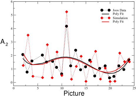
Figure 11: Joos’ experimental amplitudes in Table 7 are compared with the single simulation of 22 measurements for fixed $(N,s)$ in Table 8. By changing the pair $(N,s)$, the typical variation of each simulated entry is $(1\div 4)\cdot 10^{-3}$ depending on the sidereal time. We also show two 5th-order polynomial fits to the two different sets of values.

After this preliminary study, we have then concentrated on the real goal of our simulation, i.e. to compare with the single Joos configuration of 22 entries in Table 7. To this end, one could first try to look for the ‘best seed’, or subset of seeds, which can minimize the difference between the generated configurations and Joos’ data. This standard task, usually accomplished by minimizing a chi-square, is difficult to implement here. In fact, it is problematic to construct a function $\chi^{2}(s)$ and look for its minima because a seed $s$ and the closest seeds $s\pm 1$ give often vastly different configurations and chi-square. For this reason, we have followed an empirical procedure by forming a grid and selecting a set of seeds whose mean amplitude (for $n=24$ and $\Delta t=$ 3600 s) gets close to Joos’s mean amplitude $\langle A^{\rm joos}_{2}\rangle=1.4\cdot 10^{-3}$ for a large number $N$ of Fourier modes. One of such seeds gave a sequence $\langle A^{\rm simul}_{2}\rangle=$1.66, 1.40, 1.08, 1.21 and 1.38 (in units $10^{-3}$), for $N=10^{3}$, $10^{4}$, $10^{5}$, $10^{6}$ and $5\cdot 10^{6}$ respectively, and the configuration with $N=5\cdot 10^{6}$ was finally chosen to give an idea of the agreement one can achieve between data and a single numerical simulation for fixed $(N,s)$. The simulated values are reported in Table 8 and a graphical comparison with Joos’ data is shown in Fig. 11. We emphasize that one should not compare each individual entry with the corresponding data since, by changing $(N,s)$, the simulated instantaneous values vary typically of about $(1\div 4)\cdot 10^{-3}$ depending on the sidereal time. Instead, one should compare the overall trend of data and simulation. To this end, we show two 5th-order polynomial fits to the two different sets of values.

A more conventional comparison with the data consists in quoting for the various 22 entries simulated average values and uncertainties.

Table 9: The 2nd-harmonic amplitudes obtained by simulating the averaging process over 10 hypothetical measurements performed, at each Joos’ time, on 10 consecutive days. The stochastic velocity components are controlled by the kinematical parameters $(V,\alpha,\gamma)_{\rm CMB}$ as explained in the text. The effect of varying the pair $(N,s)$ has been approximated into a central value and a symmetric error. The mean amplitude over the 22 determinations is $\langle A^{\rm simul}_{2}\rangle=1.8\cdot 10^{-3}$.

Picture	$A^{\rm simul}_{2}[10^{-3}]~{}~{}~{}~{}$
2	$2.5\pm 1.0$
3	$1.80\pm 0.85$
4	$1.95\pm 0.85$
6	$1.90\pm 0.85$
7	$1.65\pm 0.90$
8	$2.1\pm 1.0$
9	$2.0\pm 1.0$
10	$2.2\pm 1.2$
11	$2.4\pm 1.4$
12	$2.7\pm 1.6$
13	$2.3\pm 1.5$
14	$2.4\pm 1.4$
15	$1.85\pm 0.85$
16	$1.70\pm 0.75$
17	$1.20\pm 0.75$
18	$1.20\pm 0.70$
19	$1.15\pm 0.70$
20	$1.05\pm 0.70$
21	$1.25\pm 0.60$
22	$1.55\pm 0.60$
23	$1.60\pm 0.80$
24	$1.7\pm 1.0$

To this end, we have considered the mean amplitudes $\langle A^{\rm simul}_{2}(t_{i})\rangle$ defined by averaging, for each Joos’ time $t_{i}$, over 10 hypothetical measurements performed on 10 consecutive days. For each $t_{i}$, the observed effect of varying $(N,s)$ has been summarized into a central value and a symmetric error. The values are reported in Table 9 and the comparison with Joos’ amplitudes is shown in Fig.12.

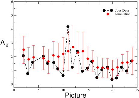
Figure 12: Joos’ experimental amplitudes in Table 7 are compared with our simulation in Table 9.

The spread of the various entries is larger at the sidereal times where the projection at Jena of the cosmic Earth’s velocity becomes larger. The tendency of Joos’ data to lie in the lower part of the theoretical predictions in Table 9 mostly depends on our use of symmetric errors. In fact, by comparing in some case with the histograms of the basic generated configurations $A^{\rm simul}_{2}(t_{i})$, we have seen that our sampling method of $\langle A^{\rm simul}_{2}(t_{i})\rangle$, based on a grid of $(N,s)$ values, typically underestimates the weight of the low-amplitude region in a prediction at the $70\%$ C.L. . This can also be checked by considering the single simulation of Table 8 and counting the sizeable fraction of amplitudes $A^{\rm simul}_{2}(t_{i})\lesssim 0.5\cdot 10^{-3}$. For this reason, one could improve the evaluation of the probability content. However, in view of the good agreement already found in Fig.12 ($\chi^{2}=13/22$), we did not attempt to carry out this more refined analysis.

In conclusion, after the first indication obtained from the fit Eq.(85), we believe that the link between Joos’ data and the Earth’s motion with respect to the CMB gets reinforced by our simulations. In fact, by inspection of Figs.11 and 12, the values of the amplitudes and the characteristic scatter of the data are correctly reproduced. In principle, there could be space for further refinements by taking into account the Earth’s orbital motion in the input values for $V$, $\alpha$ and $\gamma$.

From this agreement with the data, we then deduce that the previous value for the kinematical velocity $v\sim 217^{+66}_{-79}$ km/s, obtained by simply correcting with the helium refractive index the average observable velocity (81), has to be considerably increased if one allows for stochastic variations of the velocity field. In fact, the magnitude of the fluctuations in $v_{x}$ and $v_{y}$ is controlled by the same scalar parameter $\tilde{v}(t)\equiv\sqrt{\tilde{v}^{2}_{x}(t)+\tilde{v}^{2}_{y}(t)}$ of Eq.(34). In view of the good agreement between data and our numerical simulations, we conclude that Joos’ data are consistent with a range of kinematical velocity $v=330^{+40}_{-70}$ km/s which corresponds to Eq.(34) for $\phi=50.94^{o}$, $V=370$ km/s, $\alpha=168^{o}$ and $\gamma=-6^{o}$.

9. Summary and conclusions

The condensation of elementary quanta and their macroscopic occupation of the same quantum state is the essential ingredient of the degenerate vacuum of present-day elementary particle physics. In this description, one introduces implicitly a reference frame $\Sigma$, where the condensing quanta have ${\bf k}=0$, which characterizes the physically realized form of relativity and could play the role of preferred reference frame in a modern re-formulation of the Lorentzian approach. To this end, we have given in the Introduction some general theoretical arguments related to the problematic notions of a non-zero vacuum energy and of an exact Lorentz-invariant vacuum state. These arguments suggest the possibility of a tiny vacuum energy-momentum flux, associated with an Earth’s absolute velocity $v$, which could affect differently the various forms of matter. Namely, it could produce small convective currents in a loosely bound system such as a gas or dissipate mainly by heat conduction with no appreciable particle flow in strongly bound systems as liquid or solid transparent media. In the former case, by introducing the refractive index ${\cal N}$ of the gas, convective currents of the gas molecules would produce a small anisotropy, proportional to $({\cal N}-1)(v/c)^{2}$, of the two-way velocity of light in agreement with the general structure Eq.(23) or with its particular limit Eq.(24). Notice that this tiny anisotropy refers to the system $S^{\prime}$ where the container of the gas is at rest. In this sense, contrary to standard Special Relativity, $S^{\prime}$ might not define a true frame of rest. This conceptual possibility can be objectively tested with a new series of dedicated ether-drift experiments where two orthogonal optical resonators are filled with various gaseous media by measuring the fractional frequency shift $\Delta\nu/\nu$ between the two resonators. By assuming the typical value $v\sim 300$ km/s of most cosmic motions, one expects frequency shifts $\lesssim 10^{-10}$ for gaseous helium and $\lesssim 10^{-9}$ for air, which are well within the present technology.

Given the heuristic nature of our approach, and to further motivate the new series of dedicated experiments, we have tried to get a first consistency check. In fact, by adopting Eq.(24), the frequency shift between the optical resonators is governed by the same classical formula for the fringe shifts in the old ether-drift experiments with the only replacement

$$v^{2}\to 2({\cal N}-1)v^{2}\equiv v^{2}_{\rm obs}$$ (93)

In this way, where one re-obtains the same classical formulas (with the only replacement $v\to v_{\rm obs}$), testing the present scheme is very simple: one should just check the consistency of the true kinematical $v^{\prime}$s obtained in different experiments.

In the old times, experiments were performed with interferometers where light was propagating in gaseous media, air or helium at atmospheric pressure, where $({\cal N}-1)$ is a very small number. In this regime, the theoretical fringe shifts expected on the basis of Eqs.(23) and (24) are much smaller than the classical prediction $(v/c)^{2}$. Another important aspect of these classical experiments is that one was always expecting smooth sinusoidal modulations of the data due to the Earth’s rotation, see Eqs. (35), (37) and (38). As emphasized in Sect.2, we now understand the logical gap missed so far. The relation between the macroscopic Earth’s motions (daily rotation, annual orbital revolution,…) and the ether-drift experiments depends on the physical nature of the vacuum. Assuming Eqs.(37) and (38), to describe the effect of the Earth’s daily rotation, amounts to considering the vacuum as some kind of fluid in a state of regular, laminar motion for which global and local properties of the flow coincide. Instead, several theoretical arguments (see e.g. refs.[14, 15, 16, 17, 56, 57, 58, 59, 60]) suggest that the physical vacuum might behave as a stochastic medium similar to a turbulent fluid where large-scale and small-scale motions are only indirectly related. In this case, there might be non-trivial implications. For instance, due to the irregular behaviour of turbulent flows, vectorial observables collected at the same sidereal time might average to zero. However, this does not mean that there is no ether-drift. More generally, the relevant Earth’s motion with respect to $\Sigma$ might well correspond to that indicated by the anisotropy of the CMB, but it becomes non trivial to reconstruct the kinematical parameters from microscopic measurements of the velocity of light in a laboratory. These arguments make more and more plausible that a genuine physical phenomenon, much smaller than expected and characterized by stochastic variations, might have been erroneously interpreted as an instrumental artifact thus leading to the standard ‘null interpretation’ of the experiments reported in all textbooks.

Now, our analysis of Sects.3$-$8 shows that this traditional interpretation is far from obvious. In fact, by using Eqs.(24), (29) and (30), the small residuals point to an average velocity of about 300 km/s, as in most cosmic motions. In this alternative interpretation, the indications of the various experiments are summarized in our Table 10 .

Table 10: The average velocity observed (or the limits placed) by the classical ether-drift experiments in the alternative interpretation of Eqs.(24), (29), (30).

Experiment	gas in the interferometer	$v_{\rm obs}({\rm km/s})$	$v$(km/s)
Michelson-Morley(1887)	air	$8.4^{+1.5}_{-1.7}$	$349^{+62}_{-70}$
Morley-Miller(1902-1905)	air	$8.5\pm 1.5$	$353\pm 62$
Kennedy(1926)	helium	$<5$	$<600$
Illingworth(1927)	helium	$3.1\pm 1.0$	$370\pm 120$
Miller(1925-1926)	air	$8.4^{+1.9}_{-2.5}$	$349^{+79}_{-104}$
Michelson-Pease-Pearson(1929)	air	$4.5\pm...$	$185\pm...$
Joos(1930)	helium	$\ 1.8^{+0.5}_{-0.6}$	$330^{+40}_{-70}$

As a summary of our work, we emphasize the following points:

i) an analysis of the individual sessions of the original Michelson-Morley experiment, in agreement with Hicks [66] and Miller [65] (see our Figs. 1 and 2), gives no justification to its standard null interpretation. As discussed in Sect.3, this type of analysis is more reliable. In fact, averaging directly the fringe displacements of different sessions requires two additional assumptions, on the nature of the ether-drift as a smooth periodic effect and on the absence of systematic errors introduced by the re-adjustment of the mirrors on consecutive days, that in the end may turn out to be wrong.

ii) one gets consistent indications from the Michelson-Morley, Morley-Miller, Miller and Illingworth-Kennedy experiments. In view of this consistency, an interpretation of Miller’s observations in terms of a temperature gradient [68] is only acceptable provided this gradient represents a non-local effect as in our picture where the ether-drift is the consequence of a fundamental vacuum energy-momentum flow. We have also produced numerical simulations of the Illingworth experiment in a simple statistically isotropic and homogeneous turbulent-ether model. This represents a zeroth-order approximation and is useful to illustrate basic phenomenological features associated with the picture of the vacuum as an underlying stochastic medium. In this scheme, Illingworth’s data are consistent with fluctuations of the velocity field whose absolute scale is controlled by $\tilde{v}=V_{\rm CMB}\sim$370 km/s, the velocity of the Earth’s motion with respect to the CMB.

iii) on the other hand, there is some discrepancy with the experiment performed by Michelson, Pease and Pearson (MPP). However, as discussed in Sect.7, the uncertainty cannot be easily estimated since only a single basic MPP observation is explicitly reported in the literature. Therefore, since Miller’s extensive observations (see Fig.22 of ref.[65] and our Fig.8), within their errors, gave fluctuations of the observable velocity in the wide range 4$-$14 km/s, a single observation giving $v_{\rm obs}\sim$ 4.5 km/s cannot be interpreted as a refutation. This becomes even more true by noticing that the single session selected by Pease, within a period of several months, was chosen to represent an example of extremely small ether-drift effect.

iv) some more details are needed to account for the Joos observations. This experiment is particularly important since the data were collected at steps of 1 hour to cover the full sidereal day and were recorded by photocamera. For this reason, Joos’ experiment is not comparable with other experiments (e.g. Michelson-Morley, Illingworth) where only observations at few selected hours were performed and for which, in view of the strong fluctuations of the azimuth, one can just quote the average magnitude of the observed velocity. Moreover, differently from Miller’s, the amplitudes of all Joos’s observations can be reconstructed from the published articles [87, 88]. For these reasons, this experiment has deserved a more refined analysis and is central for our work. As discussed in Sect.8, due to uncertainties in the original data analysis, the standard 1.5 km/s velocity value quoted for this experiment should be understood as an order of magnitude estimate and not as a true upper limit. Instead, our reported observable velocity $v_{\rm obs}\sim 1.8^{+0.5}_{-0.6}$ km/s has been obtained from a direct analysis of Joos’ fringe shifts. From this value, to deduce a kinematical velocity, one still needs the refractive index. The traditional view, motivated by Miller’s review article [65] and Joos’s own statements in ref.[87], is that the experiment was performed in an evacuated housing. In these conditions, it would be easy to reconcile a large kinematical velocity $v\sim 350$ km/s with the very small values of the observable velocity. On the other hand, Swenson [90] explicitly reports that fringe shifts were finally recorded with optical paths placed in a helium bath. Since Joos’ papers do not provide any definite clue on this aspect, we have decided to follow Swenson’s indications. In this case, by simply correcting with the helium refractive index the result $v_{\rm obs}\sim 1.8^{+0.5}_{-0.6}$ km/s, one would get a kinematical velocity $v\sim 217^{+66}_{-79}$ km/s. However, as discussed in detail in Sect.8, this is only a first partial view of Joos’ experiment. In fact, by fitting the experimental amplitudes in Table 7 to various forms of cosmic motion (see Eq.(85)) we have obtained angular parameters which are very close to those that describe the CMB anisotropy (right ascension $\alpha_{\rm CMB}\sim 168^{o}$ and angular declination $\gamma_{\rm CMB}\sim-6^{o}$). Still, to get a complete agreement, one should explain the absolute normalization of the amplitudes and the strong fluctuations of the data. Thus we have improved our analysis by performing various numerical simulations where the velocity components in the plane of the interferometer $v_{x}(t)$ and $v_{y}(t)$, which determine the basic functions $C(t)$ and $S(t)$ through Eqs.(44) and the fringe shifts through Eq.(35), are not smooth functions but are represented as turbulent fluctuations. Their Fourier components in Eqs.(60) and (61) now vary within time-dependent ranges Eqs.(32)$-$(33), $[-\tilde{v}_{x}(t),\tilde{v}_{x}(t)]$ and $[-\tilde{v}_{y}(t),\tilde{v}_{y}(t)]$ respectively, controlled by the macroscopic parameters $(V,\alpha,\gamma)_{\rm CMB}$. Taking into account these stochastic fluctuations of the velocity field tends to increase the fitted average Earth’s velocity, see Eq.(89), and can reproduce correctly Joos’ 2nd-harmonic amplitudes and the characteristic scatter of the data, see Figs. 11 and 12. In view of this consistency, we conclude that the range $v=330^{+40}_{-70}$ km/s (corresponding to Eq.(34) for CMB and Joos’ laboratory) is actually the most appropriate one.

The more refined analysis adopted for the Joos experiment provides an explicit example of the previously mentioned non-trivial ingredients that might be required to reconstruct the global Earth’s motion from microscopic measurements performed in a laboratory. For this reason, the results reported in Table 10, besides providing an impressive evidence for a light anisotropy proportional to $({\cal N}-1)(v/c)^{2}$, with the realistic velocity values $v\sim$ 300 km/s of most cosmic motions, could also represent the first experimental indication for the Earth’s motion with respect to the CMB. Due to the importance of this result, and to provide the reader with all elements of the analysis, we present in a second Appendix a brief numerical simulation of one noon session of the Michelson-Morley experiment. This has been performed in the same framework adopted for the Joos experiment where the velocity components $v_{x}(t)$ and $v_{y}(t)$ in the plane of the interferometer are represented as turbulent fluctuations varying within time-dependent ranges controlled by the macroscopic parameters $(V,\alpha,\gamma)_{\rm CMB}$. We postpone to a future publication the non-trivial task of performing a complete numerical simulation of the whole Michelson-Morley experiment and of the Illingworth experiment (with its 32 sessions and the associated sets of 20 rotations for each session) where we’ll also compare the various theoretical schemes mentioned in Sect.5 to handle the stochastic components of the velocity field.

We emphasize that the simulation reported in our second Appendix corresponds to a single configuration whereas taking into account more and more configurations is essential to properly estimate theoretical uncertainties (as for the Joos experiment with the results in our Table 9 and Fig.12). Nevertheless, even this very small sample can provide interesting clues on the real data. For instance, the strong scatter of the fringe shifts at the same $\theta-$values in consecutive rotations and the good agreement with the experimental azimuths obtained by accepting Hicks’ interpretation of the observations of July 8th (see Sect.3). In this sense, this brief numerical analysis reinforces the picture of the classical experiments emerging from our Table 10. According to the usual view, the theoretical predictions, with a very low velocity $v\sim$ 30 km/s, were much larger than the observed values. Instead, in a modern view of the vacuum as a stochastic medium, theoretical predictions, for the realistic velocities $v\sim$ 300 km/s of most cosmic motions, are now well compatible and, sometimes, even smaller than the actual outcome of the observations. This latter case simply means that the experimental data were also affected by spurious effects such as deformations induced by the rotation of the apparatus or local thermal conditions. This gives a strong motivation to repeat these crucial measurements with today’s much greater accuracy.

To this end, let us now briefly consider the modern ether-drift experiments. As anticipated, in the modern experiments, the test of the isotropy of the velocity of light consists in measuring the relative frequency shift $\Delta\nu$ of two orthogonal optical resonators [35, 36]. Here, the analog of Eq.(29), for a hypothetical physical part of the frequency shift (after subtraction of all spurious effects), is

$${{\Delta\nu^{\rm phys}(\theta)}\over{\nu_{0}}}={{\bar{c}_{\gamma}(\pi/2+\theta)-\bar{c}_{\gamma}(\theta)}\over{c}}={\cal B}_{\rm medium}{{v^{2}}\over{c^{2}}}\cos 2(\theta-\theta_{0})$$ (94)

where $\theta_{0}$ is the direction of the ether-drift. This can be interpreted within Eq.(109) where

$$|{\cal B}_{\rm medium}|\sim{\cal N}_{\rm medium}-1$$ (95)

${\cal N}_{\rm medium}$ being the refractive index of the gaseous medium filling the optical resonators. Testing this prediction, requires replacing the high vacuum usually adopted within the optical resonators with a gaseous medium and studying the substantially larger frequency shift introduced with respect to the vacuum experiments.

As a rough check, a comparison was made [7, 51] with the results obtained by Jaseja et. al [95] in 1963 when looking at the frequency shift of two orthogonal He-Ne masers placed on a rotating platform. To this end, one has to preliminarily subtract a large systematic effect that was present in the data and interpreted by the authors as probably due to magnetostriction in the Invar spacers induced by the Earth’s magnetic field. As suggested by the same authors, this spurious effect, which was only affecting the normalization of the experimental $\Delta\nu$, can be subtracted by looking at the variations of the data. As discussed in refs.[7, 51], the measured variations of a few kHz are roughly consistent with the refractive index ${\cal N}_{\rm He-Ne}\sim 1.00004$ and the typical variations of an Earth’s velocity as in Eq.(52).

More recent experiments [44]$-$[50] have always been performed in a very high vacuum where, as emphasized in the Introduction, the differences between Special Relativity and the Lorentzian interpretation are at the limit of visibility. In fact, in a perfect vacuum by definition ${\cal N}_{\rm vacuum}=1$ so that ${\cal B}_{\rm vacuum}$ will vanish . Thus one should switch to the new generation of dedicated ether-drift experiments in gaseous systems. Our conclusion is that these new experiments should just confirm Joos’ remarkable observations of eighty years ago.

Acknowledgments

We thank Angelo Pagano for useful discussions.

Appendix I

To derive Eq.(24), one should start from Eq.(23) which describes light propagation in a gaseous system in the presence of convective currents of the gas molecules originating from a fundamental vacuum energy-momentum flow. Due to these convective currents, isotropy of the velocity of light would only hold if the solid container of the gas and the observer were both at rest in the particular reference frame $\Sigma$ where the macroscopic condensation of quanta correspond to the state ${\bf k}=0$. This introduces obvious differences with respect to the standard analysis. For instance, let us compare with Jauch and Watson [96] who worked out the quantization of the electromagnetic field in a moving medium of refractive index ${\cal N}$. They noticed that the procedure introduces unavoidably a preferred frame, the one where the photon energy does not depend on the direction of propagation. Their conclusion, that this frame is “usually taken as the system for which the medium is at rest”, reflects however the point of view of Special Relativity with no preferred frame. Instead, one could consider a different scenario where, at least in some limit, the angle-independence of the photon energy might only hold for some special frame $\Sigma$.

To discuss this different case, let us first consider a dielectric medium of refractive index ${\cal N}$ whose container is at rest in $\Sigma$. For an observer at rest in this reference frame, light propagation within the medium is isotropic and described by

$$\pi_{\mu}\pi_{\nu}\gamma^{\mu\nu}=0$$ (96)

where

$$\gamma^{\mu\nu}={\rm diag}({\cal N}^{2},-1,-1,-1)$$ (97)

and $\pi_{\mu}$ denotes the light 4-momentum vector for the $\Sigma$ observer. Let us now consider that the container of the medium is moving with some velocity ${\bf V}$ with respect to $\Sigma$ and is at rest in some other frame $S^{\prime}$. By analogy, light propagation within the medium for the observer in $S^{\prime}$ will be described by

$$p_{\mu}p_{\nu}g^{\mu\nu}=0,$$ (98)

where $p_{\mu}\equiv(E/c,{\bf p})$ and $g^{\mu\nu}$ denote respectively the light 4-momentum and the effective metric for $S^{\prime}$. On this basis, by introducing the $S^{\prime}$ dimensionless velocity 4-vector $u^{\mu}\equiv(u^{0},{\bf V}/c)$ (with $u_{\mu}u^{\mu}=1$), one can define a transformation matrix $A^{\mu}{{}_{\nu}}=A^{\mu}{{}_{\nu}}(u_{\mu},{\cal N})$ and express

$$g^{\mu\nu}=A^{\mu}{{}_{\sigma}}A^{\nu}{{}_{\rho}}\gamma^{\sigma\rho}$$ (99)

In this context, requiring the consistency of vacuum condensation with Special Relativity corresponds to place all reference frames on the same footing and assume $g^{\mu\nu}=\gamma^{\mu\nu}$ or

$$A^{\mu}{{}_{\nu}}(u_{\mu},{\cal N})=\delta^{\mu}_{\nu}$$ (100)

This identification is independent of the physical nature of the medium, being valid for gaseous systems as well as for liquid or solid transparent media. In this sense Special Relativity, by construction, cannot describe light propagation in the presence of a vacuum energy-momentum flow which could affect the various forms of matter differently.

Instead, consistently with the basic ambiguity in the interpretation of relativity mentioned in the Introduction, and with Lorentz’ point of view [4] (“it seems natural not to assume at starting that it can never make any difference whether a body moves through the ether or not”), one could adopt different choices without pretending to determine a priori the outcome of any ether-drift experiment. Thus, by noticing that we have at our disposal two matrices, namely $\delta^{\mu}_{\nu}$ and the Lorentz transformation matrix $\Lambda^{\mu}{{}_{\nu}}$ associated with ${\bf V}$, one could still maintain Eq.(100) for strongly bound systems, such as solid or liquid transparent media, where the small energy flux generated by the motion with respect to $\Sigma$ should mainly dissipate by heat conduction with no appreciable particle flow and no light anisotropy in the rest frame of the medium. One could instead identify

$$A^{\mu}{{}_{\nu}}(u_{\mu},{\cal N}=1)=\Lambda^{\mu}_{\nu}$$ (101)

to solve non-trivially the equation $g^{\mu\nu}=\gamma^{\mu\nu}$ when ${\cal N}=1$, i.e. when light propagates in vacuum and $\gamma^{\mu\nu}$ reduces to the Minkowski tensor $\eta^{\mu\nu}$. But then, by continuity, it is conceivable that Eq.(101), up to higher-order terms, can also describe the case ${\cal N}=1+\epsilon$ of gaseous media. This choice provides a simple interpretative model and a particular form of the more general structure Eq.(23) which corresponds to the Robertson-Mansouri-Sexl (RMS) [42, 43] parametrization for the two-way velocity of light. Moreover, when comparing with experiments with optical resonators, the resulting frequency shift is governed by the same classical formula for the fringe shifts in the old ether-drift experiments with the only replacement $V^{2}\to 2({\cal N}-1)V^{2}$. To see this, let us compute $g^{\mu\nu}$ through the relation

$$g^{\mu\nu}=\Lambda^{\mu}{{}_{\sigma}}\Lambda^{\nu}{{}_{\rho}}\gamma^{\sigma\rho}$$ (102)

with $\gamma^{\mu\nu}$ as in Eq.(97). This gives the effective metric for $S^{\prime}$

$$g^{\mu\nu}=\eta^{\mu\nu}+\kappa u^{\mu}u^{\nu}$$ (103)

with

$$\kappa={\cal N}^{2}-1$$ (104)

In this way, Eq.(98) gives a photon energy ($u^{2}_{0}=1+{\bf V}^{2}/c^{2}$)

$$E(|{\bf{p}}|,\theta)=c~{}{{-\kappa u_{0}\zeta+\sqrt{|{\bf{p}}|^{2}(1+\kappa u^{2}_{0})-\kappa\zeta^{2}}}\over{1+\kappa u^{2}_{0}}}$$ (105)

with

$$\zeta={\bf{p}}\cdot{{{\bf{V}}}\over{c}}=|{\bf{p}}|\beta\cos\theta,$$ (106)

where $\beta={{|{\bf{V}}|}\over{c}}$ and $\theta\equiv\theta_{\rm lab}$ indicates the angle defined, in the laboratory $S^{\prime}$ frame, between the photon momentum and ${\bf{V}}$. By using the above relation, one gets the one-way velocity of light

$${{E(|{\bf{p}}|,\theta)}\over{|{\bf{p}}|}}=c_{\gamma}(\theta)=c~{}{{-\kappa\beta\sqrt{1+\beta^{2}}\cos\theta+\sqrt{1+\kappa+\kappa\beta^{2}\sin^{2}\theta}}\over{1+\kappa(1+\beta^{2})}}.$$ (107)

or to ${\cal O}(\kappa)$ and ${\cal O}(\beta^{2})$

$$c_{\gamma}(\theta)\sim{{c}\over{{\cal N}}}~{}\left[1-\kappa\beta\cos\theta-{{\kappa}\over{2}}\beta^{2}(1+\cos^{2}\theta)\right]$$ (108)

From this one can compute the two-way velocity

$$\bar{c}_{\gamma}(\theta) = {{2c_{\gamma}(\theta)c_{\gamma}(\pi+\theta)}\over{c_{\gamma}(\theta)+c_{\gamma}(\pi+\theta)}}$$ (109)

$$\sim {{c}\over{{\cal N}}}~{}\left[1-\beta^{2}\left(\kappa-{{\kappa}\over{2}}\sin^{2}\theta\right)\right]$$

which, as anticipated, is a special form of the more general Eq.(23). We can then define the RMS anisotropy parameter ${\cal B}$

$${{\bar{c}_{\gamma}(\pi/2+\theta)-\bar{c}_{\gamma}(\theta)}\over{\langle\bar{c}_{\gamma}\rangle}}\sim{\cal B}{{v^{2}}\over{c^{2}}}\cos 2(\theta-\theta_{0})$$ (110)

where the pair $(v,\theta_{0})$ describes the projection of ${\bf{V}}$ onto the relevant plane and

$$|{\cal B}|\sim{{\kappa}\over{2}}\sim({\cal N}-1)$$ (111)

From the previous analysis, by replacing the two-way velocity in Eq.(28), one finally obtains the observable velocity

$$v^{2}_{\rm obs}\sim 2|{\cal B}|v^{2}\sim 2({\cal N}-1)v^{2}$$ (112)

to be used in Eq.(29). In this way, where one re-obtains the classical formulas with the only replacement $v\to v_{\rm obs}$, testing the present scheme requires to check the consistency of the kinematical $v^{\prime}$s obtained in different experiments.

Before concluding this Appendix, we emphasize that throughout this paper we have assumed the limit of a zero light anisotropy for experiments performed in vacuum. In fact, the effective metric Eq.(103) reduces to the Minkowski tensor $\eta^{\mu\nu}$ in the limit ${\cal N}\to 1$. Admittedly, this might represent a restrictive scenario and one could also consider the more general case where a metric of the form [97]

$$g^{\mu\nu}=\eta^{\mu\nu}+\Delta^{\mu\nu}$$ (113)

is introduced from the very beginning in extensions of the Standard Model. In this sense, once Eq.(113) is adopted, the vacuum behaves as a medium and the dispersion relations that describe light and particle propagation can have several solutions. For instance, light will spread with different velocities in different directions as with anisotropic media in optics. Therefore, by adopting various parameterizations for $\Delta^{\mu\nu}$, one can restrict its size by comparing with measurements of the one- and two-way velocity of light. As an example, the one-way light anisotropy reported by the GRAAL experiment [98] requires typical values of the matrix elements $|\Delta^{\mu\nu}|=10^{-13}\div 10^{-14}$ [99]. In any case, as anticipated in Sect.2, these genuine vacuum effects are much smaller than those discussed in the present paper in connection with a gas refractive index.

Appendix II

In this second Appendix we’ll report the results of a single simulation of an individual noon session of the Michelson-Morley experiment. This will be performed within the same stochastic-ether model described in Sect.8 for the Joos experiment. For sake of clarity, we recapitulate the various steps so that an interested reader can also run his own simulations.

One should first express the functions $C(t)$ and $S(t)$ as in Eqs.(44) and model the two velocity components $v_{x}(t)$ and $v_{y}(t)$ as in Eqs.(60) and (61). A basic input value is the sidereal time of the observation. This has to be inserted, together with the CMB kinematical parameters $V_{\rm CMB}\sim$ 370 km/s, $\alpha_{\rm CMB}\sim 168^{o}$, $\gamma_{\rm CMB}\sim-6^{o}$, in Eqs.(31)$-$(33) to fix the boundaries $[-\tilde{v}_{x}(t),\tilde{v}_{x}(t)]$ and $[-\tilde{v}_{y}(t),\tilde{v}_{y}(t)]$ respectively for the random parameters $x_{n}(i=1,2)$ and $y_{n}(i=1,2)$ entering Eqs.(60) and (61). In the end, with the simulated $C(t)$ and $S(t)$, one should form the fringe shift combination

$${{\Delta\lambda(\theta)}\over{\lambda}}\equiv 2C(t)\cos 2\theta+2S(t)\sin 2\theta=A_{2}(t)\cos 2(\theta-\theta_{0}(t))$$ (114)

As recalled in Sect.3, an individual session of the Michelson-Morley experiment consisted of 6 rotations. Each complete rotation of the interferometer took 6 minutes and the consecutive readings of the fringe shifts were performed every 22.5 degrees. Therefore, two consecutive readings differed by 22.5 seconds. In these conditions, a numerical simulation of a single rotation consists in generating 16 pairs $\left[C(t),S(t)\right]$ at steps of 22.5 seconds.

As the central time of the observations, we have chosen 12 A. M. of July 10, 1887 which, for Cleveland, corresponds to a sidereal time $\tau\sim 102^{o}$. To select the parameters of the simulation, we have compared with the traditional analysis of the experiment where one performs a fit to the fringe shifts obtained by averaging the results of the various experimental sessions. In our case, averaging the data of the three noon sessions in our Table 1 gives a 2nd-harmonic amplitude

$$A^{\rm fit}_{2}({\rm average~{}data-noon})\sim 0.012$$ (115)

We have thus considered the exact amplitude

$$A^{\rm exact}_{2}(t)=2\sqrt{C^{2}(t)+S^{2}(t)}$$ (116)

and selected a particular configuration whose global average over the 6 turns gives $\langle A^{\rm exact}_{2}(t)\rangle\sim$ 0.012. Of course, this condition can be realized by a very large number of configurations. These can produce very different fringe shifts at the same $\theta-$values and sizeable variations of the fitted amplitude and azimuth. Taking into account these variations is essential to perform a full numerical simulation and estimate theoretical uncertainties (as done for the Joos experiment with Table 9 and Fig.12). However, our intention here is just to give an idea of the agreement one can achieve between data and a single numerical simulation. We thus postpone to a future publication a complete analysis of the whole Michelson-Morley experiment and of the Illingworth experiment (with its 32 sessions and the associated sets of 20 rotations for each session) where we’ll also compare the various theoretical schemes mentioned in Sect.5 to handle the stochastic components of the velocity field.

The results of our single simulation for $\left[2C(t),2S(t)\right]$ are reported in Tables 11 and 12 while the combinations ${{\Delta\lambda(\theta)}\over{\lambda}}$ Eq.(114) are reported in Table 13, for $\theta={{i-1}\over{16}}~{}2\pi$ together with the results of 2-parameter fits to the simulated data. Notice the strong scatter of the simulated data at the same $\theta-$values. Of course, to compare with the real data, one should first take the even combination Eq.(50) of the entries in Table 1 which otherwise also contain odd-harmonic terms.

We conclude this brief analysis by emphasizing the importance of Hicks’ observation (see Sect.3) concerning the fringe shifts from the session of July 8th. By accepting his interpretation, the experimental azimuths from the three noon sessions of July 8th, 9th and 11th, respectively $\theta^{\rm EXP}_{0}\sim$ 357, 285 and 317 degrees, would become $\theta^{\rm EXP}_{0}\sim$ 267, 285 and 317 degrees and thus be in rather good agreement with the simulated azimuths reported in Table 13.

Table 11: The coefficients 2C(t) Eqs.(44) from a single simulation of 6 rotations in one noon session of the Michelson-Morley experiment. The stochastic components of $v_{x}(t)$ and $v_{y}(t)$ in Eqs.(60) and (61) are controlled by the kinematical parameters $(V,\alpha,\gamma)_{\rm CMB}$ as explained in the text.

i	1	2	3	4	5	6
1	$-0.023$	$+0.002$	$-0.024$	$+0.001$	$-0.004$	$-0.003$
2	$+0.003$	$-0.011$	$-0.000$	$-0.006$	$-0.021$	$-0.034$
3	$-0.001$	$-0.001$	$+0.000$	$-0.009$	$+0.002$	$+0.007$
4	$-0.002$	$+0.003$	$-0.008$	$+0.002$	$-0.060$	$-0.030$
5	$+0.002$	$-0.017$	$+0.002$	$-0.001$	$+0.003$	$-0.008$
6	$-0.007$	$-0.006$	$-0.059$	$-0.013$	$-0.008$	$-0.047$
7	$-0.020$	$-0.001$	$-0.019$	$-0.000$	$-0.003$	$-0.003$
8	$-0.011$	$-0.001$	$-0.011$	$-0.002$	$-0.026$	$+0.001$
9	$-0.015$	$-0.000$	$-0.008$	$-0.001$	$-0.008$	$-0.022$
10	$-0.037$	$-0.005$	$+0.000$	$-0.002$	$-0.003$	$+0.003$
11	$+0.003$	$-0.022$	$-0.015$	$-0.005$	$-0.003$	$+0.002$
12	$-0.002$	$-0.049$	$-0.023$	$-0.016$	$-0.009$	$-0.006$
13	$-0.001$	$+0.002$	$+0.000$	$+0.001$	$+0.003$	$-0.001$
14	$+0.003$	$-0.003$	$+0.003$	$-0.023$	$-0.001$	$-0.019$
15	$-0.012$	$-0.034$	$-0.013$	$-0.001$	$-0.001$	$-0.011$
16	$-0.004$	$-0.017$	$-0.004$	$+0.002$	$-0.010$	$-0.010$

Table 12: The coefficients 2S(t) Eqs.(44) from a single simulation of 6 rotations in one noon session of the Michelson-Morley experiment. The stochastic components of $v_{x}(t)$ and $v_{y}(t)$ in Eqs.(60) and (61) are controlled by the kinematical parameters $(V,\alpha,\gamma)_{\rm CMB}$ as explained in the text.

i	1	2	3	4	5	6
1	$+0.011$	$+0.001$	$+0.011$	$+0.000$	$+0.003$	$+0.001$
2	$+0.004$	$-0.003$	$-0.001$	$-0.008$	$+0.007$	$-0.009$
3	$+0.003$	$-0.005$	$+0.000$	$-0.007$	$+0.007$	$+0.000$
4	$+0.001$	$-0.007$	$-0.003$	$-0.001$	$+0.001$	$+0.016$
5	$+0.002$	$-0.007$	$+0.000$	$+0.001$	$-0.000$	$-0.003$
6	$-0.004$	$+0.010$	$+0.001$	$-0.001$	$+0.006$	$+0.009$
7	$-0.017$	$+0.002$	$+0.005$	$-0.000$	$-0.003$	$+0.002$
8	$+0.011$	$-0.002$	$-0.012$	$-0.001$	$+0.010$	$-0.000$
9	$+0.011$	$+0.001$	$+0.008$	$+0.011$	$+0.005$	$-0.011$
10	$+0.016$	$+0.005$	$-0.001$	$+0.001$	$-0.002$	$+0.001$
11	$+0.000$	$-0.013$	$+0.015$	$+0.005$	$-0.002$	$-0.001$
12	$-0.001$	$-0.022$	$+0.004$	$-0.003$	$-0.000$	$+0.002$
13	$-0.001$	$-0.001$	$+0.001$	$+0.000$	$-0.004$	$+0.001$
14	$-0.001$	$+0.002$	$+0.002$	$+0.018$	$+0.001$	$+0.009$
15	$-0.012$	$+0.018$	$-0.002$	$+0.001$	$-0.004$	$+0.007$
16	$+0.002$	$+0.008$	$+0.001$	$+0.002$	$-0.005$	$-0.006$

Table 13: The fringe shifts ${{\Delta\lambda(\theta)}\over{\lambda}}$ Eq.(114) for the single simulation of one noon session of the Michelson-Morley experiment reported in Tables 11 and 12. The angular values are defined as $\theta={{i-1}\over{16}}~{}2\pi$. The variance of the averages is about $\pm 0.004$ for the amplitude and about $\pm 11^{o}$ for the azimuth.

i	1	2	3	4	5	6	average
1	$-0.023$	$+0.002$	$-0.024$	$+0.001$	$-0.004$	$-0.003$	$-0.009$
2	$+0.005$	$-0.010$	$-0.001$	$-0.010$	$-0.010$	$-0.031$	$-0.010$
3	$+0.003$	$-0.005$	$+0.000$	$-0.007$	$+0.007$	$+0.000$	$-0.000$
4	$+0.002$	$-0.007$	$+0.004$	$-0.002$	$+0.043$	$+0.033$	$+0.012$
5	$-0.002$	$+0.017$	$-0.002$	$+0.001$	$-0.003$	$+0.008$	$+0.003$
6	$+0.008$	$-0.003$	$+0.041$	$+0.010$	$+0.002$	$+0.027$	$+0.014$
7	$+0.017$	$-0.002$	$-0.005$	$+0.000$	$+0.003$	$-0.002$	$+0.002$
8	$-0.016$	$+0.001$	$+0.001$	$-0.001$	$-0.025$	$+0.001$	$-0.007$
9	$-0.015$	$-0.000$	$-0.008$	$-0.001$	$-0.008$	$-0.022$	$-0.009$
10	$-0.015$	$-0.000$	$-0.000$	$-0.001$	$-0.003$	$+0.003$	$-0.003$
11	$+0.000$	$-0.013$	$+0.015$	$+0.005$	$-0.002$	$-0.001$	$+0.001$
12	$+0.000$	$+0.019$	$+0.020$	$+0.009$	$+0.006$	$+0.006$	$+0.010$
13	$+0.001$	$-0.002$	$-0.000$	$-0.001$	$-0.003$	$+0.001$	$-0.001$
14	$-0.001$	$+0.001$	$-0.004$	$+0.004$	$-0.000$	$+0.007$	$+0.001$
15	$+0.012$	$-0.018$	$+0.002$	$-0.001$	$+0.004$	$-0.007$	$-0.001$
16	$-0.005$	$-0.018$	$-0.003$	$-0.000$	$-0.004$	$-0.003$	$-0.005$
$A^{\rm fit}_{2}$	0.009	0.005	0.009	0.003	0.011	0.013	0.008
$\theta^{\rm fit}_{0}$	$279^{o}$	$259^{o}$	$266^{o}$	$285^{o}$	$255^{o}$	$272^{o}$	$269^{o}$

References

- [1] A. Einstein, Ann. der Physik, 17 (1905) 891.
- [2] H. A. Lorentz, Proceedings of the Academy of Sciences of Amsterdam, 6, 1904.
- [3] H. Poincaré, La Science et l’Hypothese, Flammarion, Paris 1902; C. R. Acad. Sci. Paris 140 (1905) 1504.
- [4] H. A. Lorentz, The Theory of Electrons, Leipzig 1909, B. G. Teubner Ed.
- [5] J. S. Bell, How to teach special relativity, in Speakable and unspeakable in quantum mechanics, Cambridge University Press 1987, pag. 67.
- [6] H. R. Brown and O. Pooley, The origin of the space-time metric: Bell’s Lorentzian pedagogy and its significance in general relativity, in ‘Physics meets Philosophy at the Planck Scale’, C. Callender and N. Hugget Eds., Cambridge University Press 2000 (arXiv:gr-qc/9908048).
- [7] M. Consoli and E. Costanzo, Phys. Lett. A333 (2004) 355.
- [8] S. Liberati, S. Sonego and M. Visser, Ann. Phys. 298 (2002) 167.
- [9] V. Scarani et al., Phys. Lett. A276 (2000) 1.
- [10] G. E. Volovik, Phys. Rep. 351 (2001) 195.
- [11] G. E. Volovik, Found.Phys. 33 (2003) 349.
- [12] S. Chadha and H. B. Nielsen, Nucl. Phys. 217 (1983) 125.
- [13] C. D. Froggatt and H. B. Nielsen, Origin of Symmetries, World Scientific, 1991.
- [14] J. A. Wheeler, in Relativity, Groups and Topology, B. S. DeWitt and C. M. DeWitt Eds., Gordon and Breach New York 1963, p. 315.
- [15] A. A. Migdal, Int. J. Mod. Phys. A9 (1994) 1197.
- [16] V. Jejjala, D. Minic, Y. J. Ng and C. H. Tze, Int. J. Mod. Phys. D19 (2010) 2311.
- [17] Y. J. Ng, Various Facets of Spacetime Foam, in Proceedings of the Third Conference on Time and Matter, Budva, Montenegro 2010, arXiv:1102.4109 [gr-qc].
- [18] G. Amelino-Camelia, Nature 418 (2002) 34.
- [19] G. Amelino-Camelia, Int.J.Mod.Phys. D11 (2002) 35.
- [20] G. Amelino-Camelia, Symmetry 2 (2010) 230.
- [21] P. Jizba and H. Kleinert, Phys. Rev. D82 (2010) 085016.
- [22] G. ’t Hooft, In Search of the Ultimate Building Blocks, Cambridge Univ. Press, 1997.
- [23] M. Consoli and P.M. Stevenson, Int. J. Mod. Phys. A15 (2000) 133, hep-ph/9905427.
- [24] M. Consoli, A. Pagano and L. Pappalardo, Phys. Lett. A318, (2003) 292.
- [25] M. Consoli and E. Costanzo, Eur. Phys. Journ. C54 (2008) 285.
- [26] M. Consoli and E. Costanzo, Eur. Phys. Journ. C55 (2008) 469.
- [27] See, for instance, R. F. Streater and A. S. Wightman, PCT, Spin and Statistics, and all that, W. A. Benjamin, New York 1964.
- [28] Y. B. Zeldovich , Sov. Phys. Usp. 11, 381 (1968).
- [29] S. Weinberg , Rev. Mod. Phys. 61, 1 (1989).
- [30] C. Barcelo, S. Liberati and M. Visser, Class. Quantum Grav. 18, 3595 (2001).
- [31] M. Visser, C. Barcelo and S. Liberati, Gen. Rel. Grav. 34, 1719 (2002).
- [32] M. Consoli, Class. Quantum Grav. 26, 225008 (2009).
- [33] R. P. Feynman, in Superstrings: A Theory of Everything ?, P. C. W. Davies and J. Brown Eds., Cambridge University Press, 1997, pag. 201.
- [34] C. Eckart, Phys. Rev. 58, 919 (1940).
- [35] For a comprehensive review, see H. Müller et al., Appl. Phys. B 77, 719 (2003).
- [36] Special Relativity, J. Ehlers and C. Lämmerzahl Eds., Lectures Notes in Physics, Springer, New York 2006.
- [37] V. W. Hughes, H. G. Robinson, and V. Beltran-Lopez, Phys. Rev. Lett. 4, 342 (1960).
- [38] R. W. P. Drever, Phil. Mag. 6, 683 (1961).
- [39] C. M. Will, The Confrontation between General Relativity and Experiment, arXiv:gr-qc/0510072.
- [40] M. Born and E. Wolf, Principles of Optics, Cambridge University Press, Cambridge 1999.
- [41] V. C. Ballenegger and T. A. Weber, Am. J. Phys.67, 599 (1999).
- [42] H. P. Robertson, Rev. Mod. Phys. 21, 378 (1949).
- [43] R. M. Mansouri and R. U. Sexl, Gen. Rel. Grav. 8, 497 (1977).
- [44] A. Brillet and J. L. Hall, Phys. Rev. Lett. 42 (1979) 549.
- [45] H. Müller et al., Phys. Rev. Lett. 91 (2003) 020401.
- [46] S. Herrmann, et al., Phys. Rev. Lett. 95 (2005) 150401.
- [47] P. Antonini et al., Phys. Rev. A71 (2005) 050101(R).
- [48] Ch. Eisele et al., Opt. Comm. 281, 1189 (2008).
- [49] S. Herrmann, et al., Phys.Rev. D 80, 105011 (2009).
- [50] Ch. Eisele, A. Newski and S. Schiller, Phys. Rev. Lett. 103, 090401 (2009).
- [51] M. Consoli and E. Costanzo, N. Cim. 119B (2004) 393.
- [52] J. Shamir and R. Fox, N. Cim. 62B (1969) 258.
- [53] R. De Abreu and V. Guerra, Relativity-Einstein’s Lost Frame, 2005, Extra]muros[ Publ.
- [54] H. Müller, Phys. Rev. D71, 045004 (2005).
- [55] J. J. Nassau and P. M. Morse, Astrophys. Journ. 65 (1927) 73.
- [56] O. V. Troshkin, Physica A168 (1990) 881.
- [57] H. E. Puthoff, Linearized turbulent flow as an analog model for linearized General Relativity, arXiv:0808.3404 [physics.gen-ph].
- [58] T. D. Tsankov, Classical Electrodynamics and the Turbulent Aether Hypothesis, Preprint February 2009.
- [59] M. Consoli, A. Pluchino and A. Rapisarda, Chaos, Solitons and Fractals 44, 1089 (2011).
- [60] M. Consoli, Phys. Lett. A 376 , 3377 (2012).
- [61] A. A. Michelson and E. W. Morley, Am. J. Sci. 34 (1887) 333.
- [62] An incomplete list of references includes: W. Sutherland, Phil. Mag. 45 (1898) 23; A. Righi, N. Cimento XVI (1918) 213; ibidem XIX (1920) 141; ibidem XXI (1921) 187; G. Dalla Noce, N. Cimento XXIV (1922) 17. Righi’s theory was also re-analyzed by P. Di Mauro, S. Notarrigo and A. Pagano, Quaderni di Storia della Fisica, 2 (1997) 101.
- [63] A. A. Michelson, et al., Astrophys. Journ. 68 (1928) pag. 341-402.
- [64] R. J. Kennedy, Phys. Rev. 47 (1935) 965.
- [65] D. C. Miller, Rev. Mod. Phys. 5 (1933) 203.
- [66] W. M. Hicks, Phil. Mag. 3 (1902) 9.
- [67] M. Born, Einstein’s Theory of Relativity, Dover Publ., New York, 1962.
- [68] R. S. Shankland et al., Rev. Mod. Phys., 27, (1955) 167.
- [69] M. A. Handshy, Am. J. of Phys. 50 (1982) 987.
- [70] E. W. Morley and D. C. Miller, Phil. Mag. 9 (1905) 680.
- [71] K. K. Illingworth, Phys. Rev. 30 (1927) 692.
- [72] H. A. Múnera, APEIRON 5 (1998) 37.
- [73] A. N. Kolmogorov, Dokl. Akad. Nauk SSSR 30 (1940) 4; English translation in Proc. R. Soc. A 434 (1991) 9.
- [74] L. D. Landau and E. M. Lifshitz, Fluid Mechanics, Pergamon Press 1959, Chapt. III.
- [75] J. C. H. Fung et al., J. Fluid Mech. 236, 281 (1992).
- [76] K. R. Sreenivasan, Rev. Mod. Phys. 71, Centenary Volume 1999, S383.
- [77] C. Beck, Phys. Rev. Lett. 98, 064502 (2007).
- [78] C. Tsallis, Introduction to Nonextensive Statistical Mechanics, Springer, 2009.
- [79] J. DeMeo, Dayton C. Miller Revisited, in Should the Laws of Gravitation be Reconsidered?, H. A. Múnera Ed., APEIRON Montreal 2011, pp. 285-315.
- [80] T. Roberts, An Explanation of Dayton Miller’s Anomalous ”Ether Drift” Result, arXiv:physics/0608238.
- [81] F. James, MINUIT: Function minimization and error analysis, CERN Computing and Networks Division, Long Writeup D506, Geneva 1994.
- [82] M. von Laue, Handbuch der Experimentalphysik, Vol. XVIII (1926) 95.
- [83] H. Thirring, Zeit. Physik 35 (1926) 723; Nature 118 (1926) 81.
- [84] A. A. Michelson, F. G. Pease and F. Pearson, Nature, 123, (1929) 88
- [85] A. A. Michelson, F. G. Pease and F. Pearson, J. Opt. Soc. Am. 18 (1929) 181.
- [86] F. G. Pease, Publ. of the Astr. Soc. of the Pacific, XLII, 197 (1930).
- [87] G. Joos, Ann. d. Physik 7 (1930) 385.
- [88] G. Joos, Naturwiss. 38 (1931) 784.
- [89] G. Joos, D. Miller, Letters to the Editor, Phys. Rev. 45, 114 (1934).
- [90] Loyd S. Swenson Jr., Journ. for the History of Astronomy, 1, 56 (1970).
- [91] A. A. Michelson, Am. J. Sci. 22, 120 (1881).
- [92] R. Tomaschek, Ann. d. Physik, 73, 105 (1924).
- [93] A. Piccard and E. Stahel, Compt. Rend. 183, 420 (1926); Naturwiss. 14, 935 (1926).
- [94] A. Piccard and E. Stahel, Compt. Rend. 185, 1198 (1927); Naturwiss. 16, 25 (1928).
- [95] T. S. Jaseja, et al., Phys. Rev. 133 (1964) A1221.
- [96] J. M. Jauch and K. M. Watson, Phys. Rev. 74, 950 (1948).
- [97] Zhou L. L. and B. -Q. Ma, Mod. Phys. Lett. A25, 2489 (2010).
- [98] V. G. Gurzadyan et al., arXiv:1004.2867 [physics.acc-ph], and references quoted therein, in Proc. 12th M. Grossmann Meeting on General Relativity, p.1495, World Sci. (2012).
- [99] Zhou L. L. and B. -Q. Ma, Astropart. Phys. 36, 37 (2012), arXiv:1009.1675 [hep-ph].