Abstract

We consider a particular case of the 3-point function of local single-trace operators in the scalar sector of planar $\mathcal{N}\!=\!4$ supersymmetric Yang-Mills, where two of the fields are $su(3)$ type, while the third one is $su(2)$ type. We show that this tree-level 3-point function can be expressed in terms of scalar products of $su(3)$ Bethe vectors. Moreover, if the second level Bethe roots of one of the $su(3)$ operators is trivial (set to infinity), this 3-point function can be written in a determinant form. Using the determinant representation, we evaluate the structure constant in the semi-classical limit, when the number of roots goes to infinity.

1 Introduction

Computing $n$-point functions of local composite gauge-invariant operators in $\mathcal{N}\!=\!4$ supersymmetric Yang-Mills theory, SYM₄, is an important problem because these $n$-point functions are among the basic objects on which the AdS/CFT correspondence can be tested . It is also a hard problem, even at tree-level, if only because of the combinatorial complexity of the operators involved. However, developments over the past few years, starting with [3] and subsequent works, raise the hope that the methods of classical and quantum integrability can be used to solve this problem, at least in the planar limit. For a comprehensive review of integrability in SYM₄ and AdS/CFT, see [4] and references therein. For shorter review, see [5].

In this work, we focus on operators $\{{\mathcal{O}}\}$ that are composed of fundamental fields in the scalar sector of SYM₄. Representing these fundamental fields as matrices in the adjoint representation of $su(N_{c})$, $\{{\mathcal{O}}\}$ are traces of products of $N_{c}\!\times\!N_{c}$ matrices. Further, in the planar limit that we are interested in, $N_{c}\rightarrow\infty$, multi-trace operators are suppressed by factors of $1/N_{c}$, and one can take $\{{\mathcal{O}}\}$ to be single-trace operators.

The weak-coupling limit

In weakly-coupled, perturbative Yang-Mills theory, the computation of the $n$-point functions is a well-defined problem. Following Okuyama and Tseng [6], it is sufficient at tree-level to count all possible planar sets of Wick contractions between the operators involved. Apart from normalization factors, the essential object in a 3-point function is the structure constant which, up to a normalisation is a tri-linear form in the Hilbert space of states, which we call the cubic vertex, in analogy with string field theory. In [7], Roiban and Volovich showed that these $n$-point functions reduce to scalar products of spin-chain states constructed using the algebraic Bethe Ansatz [8]. A systematic study in the case of three operators that belong to (different) $su(2)$ sectors was presented by Escobedo, Gromov, Sever and Vieira [9]. The tree-level correlation function of three $su(2)$ operators was expressed in [9] in terms of scalar products of off-shell Bethe states of XXX spin-$\frac{1}{2}$ chains. This method is known as “tailoring”. Furthermore, it was shown in [10] that the 3-point function can be recast in terms of scalar products of an off-shell state and an on-shell state and thereby can be evaluated in determinant form. We refer to this method as “freezing”.

The semi-classical limit

We are interested in computing the correlation functions of long operators that are dual to semi-classical string states in AdS₅ $\times$ S⁵. The semi-classical (heavy) operators $\{{\mathcal{O}}_{\textit{sc}}\}$ are associated with classical solutions of the string $\sigma$-model [11, 12, 13]. For a review see [14]. In spin-chain terms, the operators $\{\mathcal{O}_{i}\}$ are eigenstates of the spin-chain Hamiltonian. In other words, they are functions of rapidity variables that satisfy Bethe equations. For such operators, the Bethe roots condense into several cuts (macroscopic Bethe strings) in the complex rapidity plane [11]. The $n$-point functions of semiclassical operators $\{{\mathcal{O}}_{\textit{sc}}\}$ are particularly interesting, as they can be compared with the corresponding correlation functions computed on the string theory side. Computing $n$-point functions of $\{{\mathcal{O}}_{\textit{sc}}\}$ in the string theory was addressed in [15, 16, 17, 18, 19, 20, 21, 22]. However, the only case when the complete answer is known is that of two heavy and one light operators [16, 23, 24]. The same configuration (heavy-heavy-light) was considered on the gauge theory side by Escobedo et al. [25, 26], and in the $sl(2)$ sector by Georgiou [27]. They used a coherent state approximation for the two heavy operators in the $su(3)$ sector. Comparison with the Frolov-Tseytlin limit [28] of the string theory result [16, 23, 24] showed a perfect match.

The general case, when all three asymptotically-long operators are non-BPS, the complete answer for the three-point function is known only for weak coupling, and for special choice of the operators. In [29], Gromov, Sever and Vieira presented a thorough analysis of the case of one BPS and two non-BPS heavy fields from the $su(2)$ sector. In spin-chain terms, BPS operators are characterized by trivial Bethe roots that are set to infinity. The main result of [29] is an analytic contour integral derived from Korepin’s sum expression for the scalar product of two off-shell states [30]. In [31, 32], the determinant expression obtained in [10] was used to solve the problem in the general case of three heavy non-BPS operators. In [33, 34, 35], it was argued that this solution gives the 3-point function at one and two loops. At one loop this conjecture was verified in [33, 35].

Outline of contents

In Section 2, we classify the 3-point functions such that at least one operator is from the $su(3)$ sector. In 3, we recall the formulation of the $su(2)$ 3-point function, including the cubic vertex, in determinant form. In 4, we generalize the freezing method of ref.[10] to the case where two of the operators belong to $su(3)$ sectors while the third belongs to an $su(2)$ sector. Then we take one set of Bethe roots of one of the $su(3)$ operators to be trivial (sent to infinity) and use the result of [36] to write the 3-point function in a determinant form. In 5, we recall the how the $su(2)$ 3-point function was written in [31, 32, 37] in terms of certain functionals in order to be able to compute its semi-classical limit. In 6, we write the $su(3)$ 3-point function in terms of the quantities defined in the previous section. In 7, we compute the semi-classical limit of the $su(3)$ 3-point function of three non-BPS operators, under an assumption that allows us to compute the semi-classical limit of the norm of an $su(3)$ Bethe eigenstate. Appendix A contains a brief introduction to the nested coordinate Bethe Ansatz which is needed for the ‘tailoring’ approach to the $su(3)$ 3-point function. Appendix B includes details of the ‘tailoring’ approach to the $su(3)$ 3-point functions. Appendix C discusses the properties of the functional forms that are needed to obtain the semi-classical limits.

2 3-point functions with at least one $su(3)$ operator

2.1 The structure constant in ${\mathcal{N}}=4$ SYM

The 2-point and the 3-point functions are determined, up to multiplicative factors, by conformal invariance,

$$\langle{\mathcal{O}}_{i}(x_{i}){\mathcal{O}}_{j}(x_{j})\rangle=\ {L_{i}\ {\mathcal{N}}_{i}\ \delta_{ij}\over|x_{1}-x_{2}|^{2\Delta_{i}}},$$ (2.1)

$$\langle{\mathcal{O}}_{1}(x_{1}){\mathcal{O}}_{2}(x_{2}){\mathcal{O}}_{3}(x_{3})\rangle={1\over N_{c}}\ {L_{1}L_{2}L_{3}\ \sqrt{{\mathcal{N}}_{1}{\mathcal{N}}_{2}{\mathcal{N}}_{3}}\ \ \ C_{123}(\lambda)\over|x_{12}|^{\Delta_{1}+\Delta_{2}-\Delta_{3}}|x_{23}|^{\Delta_{2}+\Delta_{3}-\Delta_{1}}|x_{31}|^{\Delta_{3}+\Delta_{1}-\Delta_{2}}},$$ (2.2)

where $N_{c}$ is the number of colors, $\lambda$ is the ’t Hooft coupling and the three factors ${\mathcal{N}}_{i}$ depend on the normalization of the operators $\{{\mathcal{O}}_{i}(x_{i})\}$. The structure constant $C_{123}(\lambda)$ does not depend on the normalization.

The factors $L_{i}$, equal to the number of fundamental operators in ${\mathcal{O}}_{i}$, account for the cyclic rotations of the trace operator ${\mathcal{O}}_{i}$. The structure constant $C_{123}(\lambda)$ has the perturbative expansion

$$C_{123}(\lambda)=C^{(0)}_{123}+\lambda\ C^{(1)}_{123}+\dots\,.$$ (2.3)

To compute the tree-level structure constant $C_{123}^{(0)}$ using the method of [9], one needs the 1-loop wave functions. At 1-loop level, the operator ${\mathcal{O}}_{i}$ is represented by a Bethe eigenstate with energy $\Delta_{i}$.

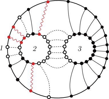
Figure 1: Planar contractions contributing to the tree-level 3-point function. The contractions $\langle X\bar{X}\rangle,\langle Y\bar{Y}\rangle$ and $\langle Z\bar{Z}\rangle$ are represented respectively by black solid lines, blue solid lines and dashed lines.

In a $su(2)$ sector, there is only one non-trivial configuration of 3-point functions. In the presence of one or more operators from an $su(3)$ sector, the structure of the 3-point functions becomes richer and we need to classify the set of possible non-trivial configurations of structure constants. An example of a set of planar contractions is given in Fig. 1. The contractions $\left\langle\,X\bar{X}\,\right\rangle$, $\left\langle\,Y\bar{Y}\,\right\rangle$ and $\left\langle\,Z\bar{Z}\,\right\rangle$ are represented respectively by solid lines, (red) wavy lines and dashed lines.

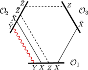
Figure 2: Schematic representation of the type-$\{2,3,3\}$ correlation function from Fig. 1.

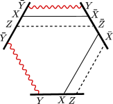
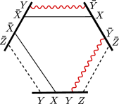
Figure 3: The two type-$\{3,3,3\}$ structure constants.

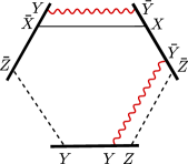
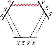
Figure 4: The remaining two type-$\{2,3,3\}$ structure constants.

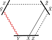
Figure 5: The type-$\{2,2,3\}$ structure constant.

Let us introduce some conventions. There are several possible choices of an $su(3)$ sector, which correspond to a choice of three distinct complex scalar fields $X$, $Y$, $Z$, $\bar{X}$, $\bar{Y}$, $\bar{Z}$, with pairs of mutually conjugated fields, like $Z$ and $\bar{Z}$, excluded. When only two types of non-conjugate scalar fields are chosen, the composite operator belongs to an $su(2)$ sector. If $\mathcal{O}_{1}$, $\mathcal{O}_{2}$ and $\mathcal{O}_{3}$ belong to $su(\alpha)$, $su(\beta)$ and $su(\gamma)$ sectors respectively, then the corresponding 3-point function of type $\{\alpha,\beta,\gamma\}$. By permutation invariance, the order of $\alpha,\beta,\gamma$ is irrelevant.

We represent the different classes of correlation functions schematically by specifying the different types of Wick contractions between pairs of operators. For example, the correlation functions corresponding to Fig. 1 belong to the class $\{2,3,3\}$ in Fig. 5. We call the operator at the bottom $\mathcal{O}_{1}$, the one at right $\mathcal{O}_{3}$ and the one at left $\mathcal{O}_{2}$. Exchanging a scalar field and its complex conjugate in all the operators does not change the value of the structure constant. This enables us to choose $\mathcal{O}_{1}$ such that it contains only the scalar fields $X,Y$ and $Z$. Since we are interested in the large $N_{c}$ limit, only planar contractions are retained.

We start by classifying the type-$\{3,3,3\}$ structure constants. In this case, there are two non-trivial inequivalent configurations, as is shown in Fig. 5. Deleting one line, that is, one type of Wick contractions, from each of these two configurations, one obtains type-$\{2,3,3\}$ structure constants. There are three such configurations, as shown in Fig. 5 and Fig. 5.

Deleting one line from the configurations in Fig. 5, one obtains a type-$\{2,2,3\}$ or a type-$\{2,2,2\}$ 3-point functions. The latter is a pure $su(2)$ 3-point function of the type studied in [9, 10, 32, 31]. There is one configuration of type-$\{2,2,3\}$, as in Fig. 5. To summarize, there are six non-trivial types of 3-point functions with at least one $su(3)$ operator.

2.2 Tailoring the tree-level structure constants

Following [9], we construct the structure constant in three steps. 1. We split the algebraic Bethe Ansatz representation of each spin chain into two: a left sub-chain and a right sub-chain. 2. Considering each spin chain to be an in-state, we “flip” each left sub-chain from an in-state to an out-state. 3. We take the scalar products of the left sub-chain state of $\mathcal{O}_{i}$ with the right sub-chain state of $\mathcal{O}_{i+1\;{\rm mod}\;3}$ $(i=1,2,3)$. Finally, we normalize the three external states. Further details on the tailoring procedure are in appendix B. We give our setup data in the table below.

Operators	Length	Rapidities	No. of Rapidities	Partitions of Rapidities
$\mathcal{O}_{1}$	$L_{1}$	$\mathbf{u}_{1},\mathbf{u}_{2}$	# $\mathbf{u}_{1}$=$N_{1}$, # $\mathbf{u}_{2}$=$M_{1}$	$\mathbf{u}^{\prime}_{1}\cup\mathbf{u}^{\prime\prime}_{1}=\mathbf{u}_{1}$, $\mathbf{u}^{\prime}_{2}\cup\mathbf{u}^{\prime\prime}_{2}=\mathbf{u}_{2}$
$\mathcal{O}_{2}$	$L_{2}$	$\mathbf{v}_{1},\mathbf{v}_{2}$	# $\mathbf{v}_{1}$=$N_{2}$, # $\mathbf{v}_{2}$=$M_{2}$	$\mathbf{v}^{\prime}_{1}\cup\mathbf{v}^{\prime\prime}_{1}=\mathbf{v}_{1}$, $\mathbf{v}^{\prime}_{2}\cup\mathbf{v}^{\prime\prime}_{2}=\mathbf{v}_{2}$
$\mathcal{O}_{3}$	$L_{3}$	$\mathbf{w}_{1},\mathbf{w}_{2}$	# $\mathbf{w}_{1}$=$N_{3}$, # $\mathbf{w}_{2}$=$M_{3}$	$\mathbf{w}^{\prime}_{1}\cup\mathbf{w}^{\prime\prime}_{1}=\mathbf{w}_{1}$, $\mathbf{w}^{\prime}_{2}\cup\mathbf{w}^{\prime\prime}_{2}=\mathbf{w}_{2}$

The lengths of the left subchains are

$$L_{13} ={\textstyle{1\over 2}}(L_{1}+L_{3}-L_{2})\;,$$ (2.4)

$$L_{12} ={\textstyle{1\over 2}}(L_{1}+L_{2}-L_{3})\;,$$

$$L_{23} ={\textstyle{1\over 2}}(L_{2}+L_{3}-L_{1})\;.$$

The structure constant reads

$$C_{123}^{(0)}=\sqrt{\frac{L_{1}L_{2}L_{3}}{\mathcal{N}_{1}\,\mathcal{N}_{2}\,\mathcal{N}_{3}}}\sum_{{\mathbf{u}}^{\prime},{\mathbf{v}}^{\prime},{\mathbf{w}}^{\prime}}{\mathrm{H}}_{F}^{\mathbf{u}}\ {\mathrm{H}}_{F}^{\mathbf{v}}\ {\mathrm{H}}_{F}^{\mathbf{w}}\ \langle{\mathbf{u}}^{\prime\prime*}|{\mathbf{v}}^{\prime}\rangle\ \langle{\mathbf{v}}^{\prime\prime*}|{\mathbf{w}}^{\prime}\rangle\ \langle{\mathbf{w}}^{\prime\prime*}|{\mathbf{u}}^{\prime}\rangle\;,$$ (2.5)

where $\mathcal{N}_{i}$ are the norms of the Bethe states:

$$\mathcal{N}_{1}=\langle{\mathbf{u}}|{\mathbf{u}}\rangle\;,\qquad\mathcal{N}_{2}=\langle{\mathbf{v}}|{\mathbf{v}}\rangle\;,\qquad\mathcal{N}_{3}=\langle{\mathbf{w}}|{\mathbf{w}}\rangle\;.$$ (2.6)

The $\mathrm{H}_{F}$ factors are given by

$$\mathrm{H}^{\mathbf{u}}_{F} =S_{1}(\mathbf{u}^{\prime\prime}_{1},\mathbf{u}_{0})\ S_{1}(\mathbf{u}^{\prime\prime}_{2},\mathbf{u}_{1})S_{2}^{>}(\mathbf{u}_{1},\mathbf{u}^{\prime\prime}_{1})S_{2}^{>}(\mathbf{u}_{2},\mathbf{u}^{\prime\prime}_{2})$$ (2.7)

$$\mathrm{H}^{\mathbf{v}}_{F} =S_{1}(\mathbf{v}^{\prime\prime}_{1},\mathbf{v}_{0})\ S_{1}(\mathbf{v}^{\prime\prime}_{2},\mathbf{v}_{1})\ S_{2}^{>}(\mathbf{v}_{1},\mathbf{v}^{\prime\prime}_{1})\ S_{2}^{>}(\mathbf{v}_{2},\mathbf{v}^{\prime\prime}_{2})$$

$$\mathrm{H}^{\mathbf{w}}_{F} =S_{1}(\mathbf{w}^{\prime\prime}_{1},\mathbf{w}_{0})\ S_{1}(\mathbf{w}^{\prime\prime}_{2},\mathbf{w}_{1})\ S_{2}^{>}(\mathbf{w}_{1},\mathbf{w}^{\prime\prime}_{1})\ S_{2}^{>}(\mathbf{w}_{2},\mathbf{w}^{\prime\prime}_{2})\;.$$

with ${{\bf u}}_{0}=\{0^{L_{1}+1}\},\;{\bf v}_{0}=\{0^{L_{2}+1}\}$ and ${\bf w}_{0}=\{0^{L_{3}+1}\}$. In the previous formula we used the following notations: we denote the scattering factors as

$$S_{\sigma}(u_{a,i},u_{b,j})=\frac{u_{a,i}-u_{b,j}+\frac{i}{2}\sigma}{u_{a,i}-u_{b,j}-\frac{i}{2}\sigma}\;,\qquad\sigma=1,2\;,$$ (2.8)

and, given a function $F(x,y)$ and two sets of variables $\mathbf{u}$, $\mathbf{v}$, we define

$$F(\mathbf{u},\mathbf{v})\equiv\prod_{u_{i}\in\mathbf{u},\;v_{j}\in\mathbf{v}}F(u_{i},v_{j}),\quad F^{>}(\mathbf{u},\mathbf{v})\equiv\prod_{i>j\atop u_{i}\in\mathbf{u},\;v_{j}\in\mathbf{v}}F(u_{i},v_{j})\;.$$ (2.9)

Proportionality factor between ABA and CBA Bethe state: $|{{\bf u}}\rangle_{\text{alg}}=c_{{\bf u}}\,|{{\bf u}}\rangle_{\text{cor}}$ is given by

$$c_{{\bf u}} = i^{N+M}\ \prod_{a=1,2}\prod_{j<k}{u_{a,j}-u_{a,k}+i\over{u_{a,j}-u_{a,k}}}.$$ (2.10)

While the formula (2.5) can be explicitly used for a small numbers of magnons, it is not adapted for taking the classical limit where the number of magnons is large. The main obstruction for taking the classical limit of (2.5) is that the scalar products involved are between off-shell states, and there is no closed form expression such as a determinant for this scalar product. In the following sections, we restrict our attention to a particular situation where the 3-point function can be written in terms of a scalar products of an off-shell state and an on-shell state.

3 The $su(2)$ cubic vertex in terms of scalar products

In preparation for the computation of the type-$\{2,3,3\}$ $su(3)$ 3-point function that we are interested in, we review an analogous computation of a type-$\{2,2,2\}$ $su(2)$ 3-point function in [10]. Consider the 3-point function of the operators ${\mathcal{O}}_{i}$, of lengths $L_{i}$, and rapidities ${{\bf u}}_{i}$ with cardinalities $N_{i}$, $i\in\{1,2,3\}$. In the following we set ${{\bf u}}_{1}={{\bf u}}$, ${{\bf u}}_{2}={\bf v}$, and ${{\bf u}}_{3}={\bf w}$. In our conventions, ${\mathcal{O}}_{1}$ consists of the fundamental fields $\{Z,X\}$, ${\mathcal{O}}_{2}$ of $\{\bar{Z},\bar{X}\}$, and ${\mathcal{O}}_{3}$ of $\{Z,\bar{X}\}$.

It is advantageous to generalize the problem slightly by introducing inhomogeneities associated with the sites of the three spin chains. Thus the $i$-th chain is characterized by inhomogeneities ${\bm{\theta}}^{(i)}=\{\theta^{(i)}_{1},\dots,\theta^{(i)}_{L_{i}}\}$, $i=1,2,3$. The three sets of inhomogeneities are not independent, because the inhomogeneities associated with two sub-chains whose fundamental fields are contracted should match. The independent inhomogeneities associated with the contractions between the $i$-th left sub-chain and the $j$-th right sub-chain are denoted by ${\bm{\theta}}^{(ij)}$. The cardinality of the set ${\bm{\theta}}^{(ij)}$ is $L_{ij}$. In this notation

$${\bm{\theta}}^{(1)}={\bm{\theta}}^{(12)}\cup{\bm{\theta}}^{(13)},\ {\bm{\theta}}^{(2)}={\bm{\theta}}^{(12)}\cup{\bm{\theta}}^{(23)},\ {\bm{\theta}}^{(3)}={\bm{\theta}}^{(13)}\cup{\bm{\theta}}^{(23)}.$$ (3.1)

The planarity of the $\langle Z\bar{Z}\rangle$ contractions between the operators ${\mathcal{O}}_{2}$ and ${\mathcal{O}}_{3}$ and the $\langle X\bar{X}\rangle$ contractions between the operators ${\mathcal{O}}_{1}$ and ${\mathcal{O}}_{3}$ selects the component of ${\mathcal{O}}_{3}$ with $N_{3}=L_{13}$ successive $\bar{X}$’s and $L_{3}-N_{3}$ successive $Z$’s, as in Fig. 1. Consequently, the correlation function is given by the product of two factors:

• The probability to find the component ${\rm Tr}[Z^{L_{23}}\bar{X}^{L_{13}}]$ in the state $|{\bf w}\rangle$.

• The contribution of the remaining contractions can be recast as the scalar product of an on-shell state of rapidities ${{\bf u}}$ and an off-shell state of rapidities ${\bf v}$, in a spin chain of length $L_{1}$.

We present below the derivation of the two factors using the language of the six-vertex model.

3.1 The $su(2)$ Bethe states as six-vertex-model partition functions

The three type of vertex configurations, $a$, $b$, $c$ represented in Fig. 6 have weights

$$a(u-z)=\frac{u-z+i}{u-z}\;,\quad b(u-z)=1\;,\quad c(u-z)=\frac{i}{u-z}.$$ (3.2)

The rapidities $u$ and $z=\theta+i/2$ are associated respectively with the horizontal and with the vertical lines. These weights are given by the three types of non-zero elements of the $L$-matrix, which in our case coincides with the $R$-matrix,

$${L}(u-z)={\bf I}+\frac{i}{u-z}\ {\bf P}\;,\qquad z=\theta+i/2.$$ (3.3)

Here ${\bf I}$ is the identity matrix and ${\bf P}$ is the permutation matrix.

Figure 6: Graphical representation of the six non-zero elements of the $L$ -matrix (3.3). The rapidity $u$ is associated with the horizontal line, while the rapidity $z=\theta+i/2$ is associated with the vertical line.

Consider the expansion of a Bethe vector $|{{\bf u}}\rangle$ in the local basis $|s_{1},\dots,s_{L}\rangle$, where $s_{k}\in\{1,2\}$,

$$|{{\bf u}}\rangle=\sum_{s_{1},\ldots,s_{L}=1,2}\psi_{s_{1},\ldots,s_{L}}({{\bf u}})|{s_{1},\ldots,s_{L}}\rangle\,.$$ (3.4)

Each of the components $\psi_{s_{1},\ldots,s_{L}}({{\bf u}})$ is a sum over all the possible vertex configurations with on a $L\times N$ rectangle, with all indices fixed to 1 on the left and the upper boundaries, 2 on the right boundary, and free indices equal to $s_{1},\ldots,s_{L}$ on the lower boundary, as shown in Fig. 8. Similarly the dual Bethe state is represented by the partition function of the six-vertex model on a rectangle, with boundary conditions 1 on the right and the lower boundary, and 2 on the left boundary.

3.2 The $su(2)$ scalar/ inner product in terms of the 6-vertex model

With the normalisation of the basis

$$\left\langle\,s_{1},\dots,s_{L}|r_{1},\dots,r_{L}\,\right\rangle=\delta_{s_{1},r_{1}}\dots\delta_{s_{L},r_{L}}\,,$$ (3.5)

the scalar product of two (in general off-shell) Bethe states

$$\langle{\bf v}|{{\bf u}}\rangle=\sum_{s_{1},\dots,s_{L}=1,2}\psi_{s_{1}\dots s_{L}}({{\bf u}})\ \psi_{s_{1}\dots s_{L}}({\bf v})^{*}$$ (3.6)

is obtained simply by gluing two such partition functions, as shown in Fig. 8, and summing over the free indices. In addition to the sesquilinear form (3.6), which is ‘the scalar product’ , we define a bilinear form, which we call ‘the inner product’ 

$$\langle{\bf v},{{\bf u}}\rangle=\langle{\bf v},{{\bf u}}\rangle=\sum_{s_{1},\dots,s_{L}=1,2}\psi_{s_{1}\dots s_{L}}({{\bf u}})\ \psi_{s_{L}\dots s_{1}}({\bf v}).$$ (3.7)

The vertex representation of the inner product (3.7) is obtained by gluing two lattices as the one shown in Fig. 8 and summing over the free spin indices. The result is the six-vertex partition function on a lattice with indices $1^{L}$ on the upper and lower boundaries, and $1^{N}2^{N}$ on the left and right boundaries in Fig. 8. The symmetry $\langle{\bf v},{{\bf u}}\rangle=\langle{\bf v},{{\bf u}}\rangle$ of the inner product follows from the symmetry of the weights $a,b,c$ of the vertices in Fig 6 with respect to a rotation by 180 degrees.

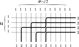
Figure 7: A six-vertex configurations for the coefficient $\psi_{{}_{121221211111}}({{\bf u}})$ of the Bethe state $|{{\bf u}}\rangle$, Eq. (3.4).

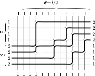
Figure 8: A six-vertex configurations for the inner product $\left\langle\,{\bf v},{{\bf u}}\,\right\rangle$.

It follows from the hermitian conjugation properties of the creation ($B$) and the annihilation ($C$) operators (see the historical note [38]) that for $N$-magnon states

$$\langle{\bf v}|{{\bf u}}\rangle=(-1)^{N}\ \left\langle\,{\bf v}^{*},{{\bf u}}\,\right\rangle,$$ (3.8)

where the set of rapidities ${\bf v}^{*}$ is obtained from ${\bf v}$ by complex conjugation. Since the Hamiltonian of the XXX chain is hermitian, the sets of rapidities of the Bethe eigenstates are symmetric under complex conjugation. Therefore the normalisation factor ${\mathcal{N}}_{1}=|\left\langle\,{{\bf u}},{{\bf u}}\,\right\rangle|$ in (2.1) is equal to the (squared) norm $\left\langle\,{{\bf u}}|{{\bf u}}\,\right\rangle$ of the Bethe eigenstate.

The structure constant $C^{(0)}_{123}$ is equal, up to the normalization factor, to the cubic vertex made of the wave functions of the Bethe states in the representation (3.4),

$$C^{(0)}_{123}={\left\langle\,{{\bf u}},{\bf v},{\bf w}\,\right\rangle\over\sqrt{\left\langle\,{{\bf u}},{{\bf u}}\,\right\rangle\left\langle\,{\bf v},{\bf v}\,\right\rangle\left\langle\,{\bf w},{\bf w}\,\right\rangle}}\,,$$ (3.9)

where the form of the cubic vertex depends on the choice of the three $su(2)$ sectors. In our particular case

$$\left\langle\,{{\bf u}},{\bf v},{\bf w}\,\right\rangle \equiv \sum\psi_{{\underbrace{{}_{1\dots 1}}_{L_{23}}}s_{{L_{12}}}\dots s_{1}}({\bf v})\ \psi_{s_{1}\dots s_{L_{12}}\underbrace{{}_{2\dots 2}}_{L_{13}}}({{\bf u}})\ \ \psi_{\underbrace{{}_{2\dots 2}}_{L_{13}}\underbrace{{}_{1\dots 1}}_{L_{23}}}({\bf w})\,,$$ (3.10)

where the summation indices $s_{1},\dots s_{L_{12}}$ take values $1$ and $2$.

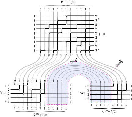
Figure 9: The $su(2)$ cubic vertex in terms of six-vertex configurations. The shaded area factorizes out and can be cut out. Furthermore, the right piece is connected to the rest only with type-2 contractions and factorizes out. The lattice splits into two pieces which do not talk to each other and can be evaluated separately.

The cubic vertex $\left\langle\,{{\bf u}},{\bf v},{\bf w}\,\right\rangle$ can be evaluated using the fact that it gives the partition function of the six-vertex model on a lattice obtained by gluing three rectangular lattices with dimensions $L_{1}\times N_{1}$, $L_{2}\times N_{2}$ and $L_{3}\times N_{3}$ as shown in Fig. 9. The indices $1$ and $2$ are identified with $Z$ and $X$ or their complex conjugates, depending on the operator under consideration. First we notice that in the part of the lattice that has vertical lines labeled by ${\bm{\theta}}^{(23)}$, represented by the shaded area in Fig. 9, there is only one six-vertex configuration, and therefore its contribution to the cubic vertex factorizes out. The factor is a pure phase if the sets ${\bf v}$ and ${\bm{\theta}}^{(23)}$ are symmetric under complex conjugation. We will assume that this is the case and will ignore this phase factor. Therefore we can delete this part of the lattice.

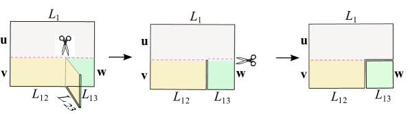
Figure 10: Schematic representation of the lattice obtained by gluing the rectangular lattices corresponding to the states $\langle{{\bf u}}|$, $|{\bf v}\rangle$ and $|{\bf w}\rangle$, with subsequent removal of the redundant piece and separating the two non-interacting sub-lattices. After the removal of the redundant piece, the states $|{\bf v}\rangle$ and $|{\bf w}\rangle$ are no more Bethe eigenstates, because the chain are shortened ($L_{1}\to L_{12}$ and $L_{3}\to L_{23}$).

Next, we observe that the sub-lattice associated with the operator ${\mathcal{O}}_{3}$ factorizes because all lines that connect it with the rest of the lattice are of type 2. (This factorisation is obvious in the expression (3.10) for the cubic vertex.) These operations are schematically represented in Fig. 10.

The problem boils down to the calculation of two independent six-vertex partition functions, which give the two non-trivial factors in the structure constant. These two factors will be computed using the freezing procedure. The freezing procedure for the first factor works as follows. One starts from a rectangular lattice corresponding to the scalar product $\left\langle\,\tilde{\bf v}|{{\bf u}}\,\right\rangle$. Both sets of rapidities have cardinality $N_{1}$. The first $N_{2}$ rapidities $\tilde{\bf v}$ coincide with the rapidities ${\bf v}$ characterizing the operator ${\mathcal{O}}_{3}$, the rest $N_{3}=N_{1}-N_{2}=L_{1}-L_{12}$ of the rapidities $\tilde{\bf v}$ will be denoted by $\tilde{v}_{N_{2}+1}=\tilde{z}_{L_{12}+1},\dots,\tilde{v}_{N_{1}}=\tilde{z}_{L_{1}}$, or symbolically, $\tilde{\bf v}={\bf v}\cup\tilde{{\bf z}}$.

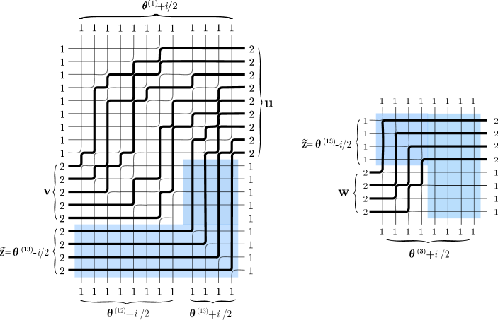
Figure 11: The freezing procedure for the two factors in $C_{123}^{0}$

3.3 The $su(2)$ freezing procedure

If we adjust the rapidity of the last magnon to the value of the last inhomogeneity, $\tilde{z}_{L_{1}}=\theta_{L_{1}}-i/2$, then the vertex at the low right corner is necessarily of type $c$. Then the only possibility for the rest of the vertices on the last row and the last column is that they are type $b$. This is what we call “freezing". Hence last row and the last column form a hooked index line carrying the index $2$, as shown in Fig. 11, left. This procedure is repeated $N_{3}$ times, the rapidities of the lowest $N_{3}$ rows fixed to $\tilde{{\bf z}}={\bm{\theta}}^{(13)}-i/2$. The result is that the rightmost $N_{3}$ indices below the lowest horizontal $u$-line are fixed to the value $2$. After removing the frozen part of the lattice, shaded in blue in the figure, we obtain that the first factor in the cubic vertex equals the scalar product $\left\langle\,{\bf v}\cup\tilde{{\bf z}},{{\bf u}}\,\right\rangle$. The contribution of the frozen part of the lattice is the product of all $c$-vertices on the diagonal, which equals $(-1)^{L_{13}}$, a factor we will ignore.

In a similar way we compute the second factor . The freezing procedure is shown in Fig. 11, right. We start with a scalar product $\left\langle\,{\bf w},\tilde{{\bf z}}\,\right\rangle$ for a chain of length $L_{3}=N_{3}+L_{23}$. We freeze the rapidities of the bra state to $\tilde{{\bf z}}={\bm{\theta}}^{(13)}-i/2$. The frozen area (shaded in blue) gives a contribution, which is a pure phase if both sets ${\bf w}$ and ${\bm{\theta}}^{(23)}$ are symmetric under complex conjugation. We will assume that this is the case and will ignore this factor. The rest of the lattice gives the second factor in the expression for the cubic vertex. We find

$$\left\langle\,{{\bf u}},{\bf v},{\bf w}\,\right\rangle=\langle{\bf v}\cup\tilde{{\bf z}},{{\bf u}}\rangle_{{\bm{\theta}}^{(1)}}\ \langle{\bf w},\tilde{{\bf z}}\rangle_{{\bm{\theta}}^{(3)}}$$ (3.11)

up to a factor which takes into account the contribution of the deleted and added pieces of the lattice. This factor is a pure phase, since the set ${\bf w}$ is symmetric under complex conjugation, and can be ignored.

4 The $su(3)$ cubic vertex in terms of scalar products

As before, we consider that the three operators, ${\mathcal{O}}_{1},\ {\mathcal{O}}_{2},\ {\mathcal{O}}_{3}$, are described by three sets of rapidities ${{\bf u}}=\{{{\bf u}}_{1},{{\bf u}}_{2}\},\ {\bf v}=\{{\bf v}_{1},{\bf v}_{2}\}$ and ${\bf w}=\{{\bf w}_{1},{\bf w}_{2}\}$ with cardinalities respectively $N_{1}+M_{1},N_{2}+M_{2}$ and $N_{3}+M_{3}$. In the configuration we are considering, ${\bf w}_{2}=\emptyset$, since ${\mathcal{O}}_{3}$ is an $su(2)$ operator. We refer to Section 6 for the equations obeyed by these rapidities.

Again, we have two types of contributions to the correlation function:

• the contribution of the $\langle Z\bar{Z}\rangle$ contractions between the operators ${\mathcal{O}}_{2}$ and ${\mathcal{O}}_{3}$, through the factor $\langle\tilde{{\bf z}}_{1},{\bf w}_{1}\rangle$, with $\tilde{{\bf z}}_{1}={\bm{\theta}}^{(13)}-i/2$ and $\#\tilde{{\bf z}}_{1}=N_{3}$,

• the remaining contractions, which can be recast as the inner product $\langle{\bf v}\cup\tilde{{\bf z}},{{\bf u}}\rangle$ between an on-shell vector of a spin chain with length $L_{1}$ and rapidities ${{\bf u}}=\{{{\bf u}}_{1},{{\bf u}}_{2}\}$ and an off-shell state with the same length and rapidities $\left({\bf v}=\{{\bf v}_{1},{\bf v}_{2}\}\right)\cup\left(\tilde{{\bf z}}=\{\tilde{{\bf z}}_{1},\tilde{{\bf z}}_{2}\}\right)$, with $\tilde{{\bf z}}_{1}={\bm{\theta}}^{(13)}-i/2$ and $\tilde{{\bf z}}_{2}={\bm{\theta}}^{(13)}-i$.

Below we evaluate, using the freezing argument, the $\{2,3,3\}$ type structure constant (Fig. 1),

$$C^{(0)}_{123}={\left\langle\,{{\bf u}},{\bf v},{\bf w}_{1}\,\right\rangle^{{{}^{su(3)}}}\over\sqrt{\left\langle\,{{\bf u}},{{\bf u}}\,\right\rangle^{{}^{su(3)}}\left\langle\,{\bf v},{\bf v}\,\right\rangle^{{}^{su(3)}}\left\langle\,{\bf w}_{1},{\bf w}_{1}\,\right\rangle}}\,.$$ (4.1)

We will show that the corresponding cubic vertex is given by

$$\left\langle\,{{\bf u}},{\bf v},{\bf w}\,\right\rangle^{{{}^{su(3)}}} = \langle{\bf v}\cup\tilde{{\bf z}},{{\bf u}}\rangle_{{\bm{\theta}}^{(1)}}^{{}^{{}^{su(3)}}}\ \langle{\bf w}_{1},\tilde{{\bf z}}_{1}\rangle_{{\bm{\theta}}^{(3)}}$$ (4.2)

$${\rm with}\quad\quad\tilde{{\bf z}} = \{\tilde{{\bf z}}_{1},\tilde{{\bf z}}_{2}\}=\{{\bm{\theta}}^{(13)}-i/2,\ {\bm{\theta}}^{(13)}-i\}.$$ (4.3)

Here $\langle\ \ ,\ \ \rangle$ denotes, as before, the $su(2)$ inner product, and $\langle\ \ ,\ \ \rangle^{{}^{su(3)}}$ denotes the $su(3)$ inner product.

4.1 The $su(3)$ Bethe states in terms of the 15-vertex-model

In order to generalize the freezing procedure to $su(3)$, let us first show how to represent the components of the $su(3)$ Bethe vectors in terms of configurations of a 15-vertex model shown in Fig. 12. The vertices are similar to those from Fig. 6, with the difference that the indices carried by the lines can be now $1,2$ or $3$. We represent them graphically by thin, red and black lines, respectively. The weights are identical to those from equation (3.2), depending on whether the indices carried by the lines are equal or different.

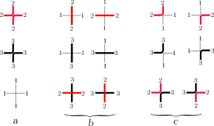
Figure 12: Graphical representation of the 15 non-zero elements of the $su(3)$ $L$ -matrix, Eq. (3.3). The rapidities $u$ and $z=\theta+i/2$ are associated with the horizontal and the vertical lines, respectively.

The Bethe vector $|{{\bf u}}\rangle$ is given by the expansion

$$|{{\bf u}}\rangle=\sum_{s_{1},\ldots,s_{L}=1}^{3}\psi_{s_{1},\ldots,s_{L}}({{\bf u}})\ |{s_{1},\ldots,s_{L}}\rangle$$ (4.4)

where $\psi_{s_{1},\ldots,s_{L}}({{\bf u}})$ is a sum over all the possible 15-vertex configurations on a rectangular lattice with $L_{1}+N_{1}$ vertical lines and $N_{1}+M_{1}$ horizontal lines, with the free spin indices equal to $s_{1},\ldots,s_{L}$. An example for such a vertex configuration is given in Fig. 13. The first $L_{1}$ vertical lines carry rapidities $\theta^{(1)}_{1}+i/2,\ldots,\theta^{(1)}_{L_{1}}+i/2$ and spin indices $1$ on the top, which correspond to the vacuum $|\Omega\rangle=|1^{L}\rangle\equiv|11\ldots 1\rangle$. The right $N_{1}$ vertical lines carry rapidities $u_{1,1}+i\ldots u_{1,N_{1}}+i$ and have index $2$ on the top. At the bottom, the first $L_{1}$ indices are free, and the last $N_{1}$ ones are fixed to $1$. The lower $N_{1}$ horizontal line correspond to the first-level magnons and carry rapidities $u_{1,1},\dots,u_{1,N_{1}}$. The higher $M_{1}$ horizontal lines represent the second-level magnons with rapidities $u_{2,1},\dots,u_{2,M_{1}}$. Due to the particular spin and rapidity choices, the shaded regions are frozen to the particular configuration shown in the Figure. This diagram is equivalent to (a special case of) the one used by Reshetikhin in [39].

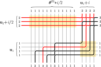
Figure 13: A configuration contributing to the coefficient $\psi_{131231311111}({{\bf u}})$ of a $su(3)$ Bethe vector (4.4) with $L=12$, $N=4$ and $M=3$ .

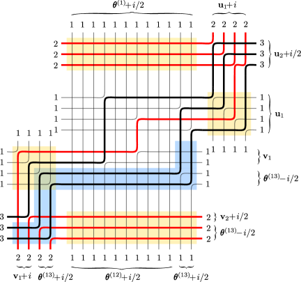
Figure 14: The inner product $\langle\tilde{\bf v},{{\bf u}}\rangle$ and the freezing to $\langle{\bf v}\cup{\bm{\theta}}^{(13)}-i/2,{{\bf u}}\rangle$ .

The structure constant factorizes as in the $su(2)$ case. The two factors can be cast in the form of scalar products of an on-shell and an off-shell Bethe states by applying the freezing procedure.

4.2 The $su(3)$ freezing procedure

Consider the scalar product of two $su(3)$ states of the first chain, $\langle\tilde{\bf v},{{\bf u}}\rangle$=$\langle\{\tilde{\bf v}_{1},\tilde{\bf v}_{2}\},\{{{\bf u}}_{1},{{\bf u}}_{2}\}\rangle$, as represented in figure 14. Our purpose is to freeze the rightmost $N_{3}$ indices to the value $3$, as imposed by the planarity of the contractions in the three point function. This can be done by setting the last $N_{3}$ rapidities of first level magnons at their freezing values,

$$\tilde{v}_{1,N_{2}+1}=\theta^{(13)}_{1}-i/2,\ \ldots,\ \tilde{v}_{1,N_{1}}=\theta^{(13)}_{N_{3}}-i/2.$$ (4.5)

This will insure that the corresponding frozen region contains only red and black lines propagating from the top to the bottom of the diagram. The number of black or red lines is not fixed by the freezing, only their sum is fixed. In order to force all the lines in the frozen region to be black, we have to apply once again the freezing procedure to the magnons of second level, by fixing

$$\tilde{v}_{2,M_{2}+1}=\theta^{(13)}_{1}-i,\ \ldots\ \tilde{v}_{2,M_{1}}=\theta^{(13)}_{N_{3}}-i.$$ (4.6)

The remaining magnons are set to the corresponding values in the state $|{\bf v}\rangle$,

$$\tilde{v}_{1,1}=v_{1,1},\ \ldots,\ \tilde{v}_{2,M_{2}}=v_{2,M_{2}}.$$ (4.7)

This gives us the first factor of the expression (4.2) for the cubic vertex. The second factor, $\left\langle\,{{\bf z}}_{1},{\bf w}_{1}\,\right\rangle$, is the same as in the $su(2)$ case.

5 The $su(2)$ structure constant in terms of the ${\mathscr{A}}$-functional

In the $su(2)$ case, the rapidities of the on-shell Bethe states satisfy the Bethe equations

$$\prod_{l=1}^{L}{u_{j}-\theta_{l}+i/2\over u_{j}-\theta_{l}-i/2}=-\prod_{k=1}^{N}{u_{j}-u_{k}+i\over u_{j}-u_{k}-i}\,,\quad j=1,\dots,N.$$ (5.1)

The Bethe equations (5.1) follow from the requirement that the eigenvalue $T(u)$ of the $T$-matrix,

$$T(u)={Q_{\bm{\theta}}^{+}(u)\over Q^{-}_{\bm{\theta}}(u)}{Q^{--}_{{\bf u}}(u)\over Q_{{\bf u}}(u)}+{Q^{++}_{{\bf u}}(u)\over Q_{{\bf u}}(u)}\equiv e^{ip_{{\bf u}}^{1}(u)}+e^{ip^{2}_{{\bf u}}(u)}$$ (5.2)

has vanishing residues at the Bethe roots. Here $Q_{{\bf u}}$ and $Q_{\bm{\theta}}$ are the Baxter polynomials

$$Q_{{\bf u}}(u)=\prod_{j=1}^{N}(u-u_{j}),\qquad Q_{{\bm{\theta}}}(u)=\prod_{l=1}^{L}(u-\theta_{l}),$$ (5.3)

and

$$Q^{\pm}(u)=Q(u\pm i/2),\ \ Q^{\pm\pm}(u)=Q(u\pm i),\quad Q^{[n]}(u)=Q(u+in/2).$$ (5.4)

The Bethe equations read

$$e^{2ip_{{\bf u}}(u_{j})}=-1,\qquad j=1,\dots,N,$$ (5.5)

where the pseudomomentum $p_{{\bf u}}$, known also as the counting function, is defined modulo $\pi$ by

$$e^{2ip_{{\bf u}}}=e^{ip^{1}_{{\bf u}}-ip^{2}_{{\bf u}}}={Q_{\bm{\theta}}^{-}\over Q^{+}_{\bm{\theta}}}\ {Q^{++}_{{\bf u}}\over Q^{--}_{{\bf u}}}\,.$$ (5.6)

The $T$-matrix (5.2) is normalized according to the vertex representation with weights (3.2). The eigenvalues of the diagonal elements of the monodromy matrix on the vacuum, $A(u)$ and $D(u)$, are given by

$$\begin{aligned} D(u)&=e^{ip^{1}_{\emptyset}(u)}=\prod_{l=1}^{L}b(u-\theta_{l}-i/2)=1,\\ A(u)&=e^{ip^{2}_{\emptyset}(u)}=\prod_{l=1}^{L}a(u-\theta_{l}-i/2)={Q_{\bm{\theta}}^{+}(u)\over Q^{-}_{\bm{\theta}}(u)}.\end{aligned}$$ (5.7)

The inner product of an on-shell Bethe state ${{\bf u}}$ and an off-shell state ${\bf v}$ is given in a determinant form by [40][41]

$$\left\langle\,{\bf v},{{\bf u}}\,\right\rangle = \ \prod_{j=1}^{N}A_{\bm{\theta}}(v_{j})\ {\mathscr{S}}_{{{\bf u}},{\bf v}}\,,$$ (5.8)

where

$${\mathscr{S}}_{{{\bf u}},{\bf v}} = {\det_{jk}\Omega(u_{j},v_{k})\over\det_{jk}{1\over u_{j}-v_{k}+i}}\,,$$ (5.9)

is the Slavnov determinant. The Slavnov kernel $\Omega(u,v)$ is defined by

$$\Omega(u,v)=t(u-v)-e^{2ip_{{\bf u}}(v)}\ t(v-u)\,,\qquad t(u)={1\over u}-{1\over u+i}\,.$$ (5.10)

The Slavnov determinant cannot be directly evaluated in the classical limit. This can be done using the representation in terms of the ${\mathscr{A}}$-functional introduced in [29]. The Slavnov determinant ${\mathscr{S}}_{{{\bf u}},{\bf v}}$ was expressed in terms of the ${\mathscr{A}}$-functional first for the limit ${{\bf u}}\to\infty$ [29] and then in the general case [32][31]. Later a more compact expression was found in [37].

The ${\mathscr{A}}$-functional, whose properties are listed in Appendix C, is defined for any function $f(u)$ and any set of points in the complex plane ${{\bf u}}=\{u_{1},\dots,u_{N}\}$ as follows,

$${\mathscr{A}}^{\pm}_{{\bf u}}[f] = {\det_{jk}\left(u_{j}^{k-1}-f(u_{j})\,(u_{j}\pm i)^{k-1}\right)\over\det_{jk}\left(u_{j}^{k-1}\right)}\,.$$ (5.11)

The Slavnov determinant is expressed in terms of this functional as [37]

$${\mathscr{S}}_{{{\bf u}},{\bf v}}=(-1)^{N}\ {\mathscr{A}}^{+}_{{{\bf u}}\cup{\bf v}}[{Q^{-}_{\bm{\theta}}\over Q^{+}_{\bm{\theta}}}].$$ (5.12)

Let us express the scalar products in the expression for the cubic vertex in terms of the ${\mathscr{A}}$-functional. We find for the two inner products in (4.2)

$$\langle{\bf v}\cup\tilde{{\bf z}},{{\bf u}}\rangle_{{\bm{\theta}}^{(1)}} = (-1)^{N_{1}}{\prod_{j=1}^{N_{2}}A(v_{j})\prod_{j=1}^{N_{3}}A(\tilde{z}_{j})}\ \ {\mathscr{A}}^{+}_{{\bf v}\cup{{\bf u}}}[{Q^{-}_{{\bm{\theta}}^{(12)}}\over Q^{+}_{{\bm{\theta}}^{(12)}}}]\,,$$ (5.13)

$$\langle{\bf w},\tilde{{\bf z}}\rangle_{{\bm{\theta}}^{(3)}}\ \ \ = (-1)^{N_{3}}\prod_{j=1}^{N_{3}}A(\tilde{z}_{j})\ \ {\mathscr{A}}^{+}_{\bf w}[{Q^{+}_{{\bm{\theta}}^{(23)}}\over Q^{-}_{{\bm{\theta}}^{(23)}}}].$$ (5.14)

Proof: Using the properties of the ${\mathscr{A}}$-functional (Appendix C), we transform

$${\mathscr{A}}^{+}_{{\bf v}\cup\tilde{{\bf z}}\cup{{\bf u}}}[{Q^{-}_{{\bm{\theta}}^{(1)}}\over Q^{+}_{{\bm{\theta}}^{(1)}}}] = {\mathscr{A}}^{+}_{{\bf v}\cup\tilde{{\bf z}}\cup{{\bf u}}}[{Q^{-}_{{\bm{\theta}}^{(13)}}\over Q^{+}_{{\bm{\theta}}^{(13)}}}{Q^{-}_{{\bm{\theta}}^{(12)}}\over Q^{+}_{{\bm{\theta}}^{(12)}}}]={\mathscr{A}}^{+}_{{\bf v}\cup{{\bf u}}}[{Q^{-}_{{\bm{\theta}}^{(12)}}\over Q^{+}_{{\bm{\theta}}^{(12)}}}],$$ (5.15)

$${\mathscr{A}}^{+}_{{\bf w}\cup\tilde{{\bf z}}}[{Q^{-}_{{\bm{\theta}}^{(3)}}\over Q^{+}_{{\bm{\theta}}^{(3)}}}] = {\mathscr{A}}^{+}_{{\bf w}\cup\tilde{{\bf z}}}[{Q^{-}_{{\bm{\theta}}^{(13)}}\over Q^{+}_{{\bm{\theta}}^{(13)}}}{Q^{-}_{{\bm{\theta}}^{(23)}}\over Q^{+}_{{\bm{\theta}}^{(23)}}}]={\mathscr{A}}^{+}_{\bf w}[{Q^{-}_{{\bm{\theta}}^{(23)}}\over Q^{+}_{{\bm{\theta}}^{(23)}}}].$$ (5.16)

Ignoring the factors that are pure phases, we find for the cubic vertex

$$\left\langle\,{{\bf u}},{\bf v},{\bf w}\,\right\rangle^{{}^{su(3)}}={\mathscr{A}}^{+}_{{\bf v}\cup{{\bf u}}}[{Q^{-}_{{\bm{\theta}}^{(12)}}\over Q^{+}_{{\bm{\theta}}^{(12)}}}]\ {\mathscr{A}}^{+}_{\bf w}[{Q^{-}_{{\bm{\theta}}^{(23)}}\over Q^{+}_{{\bm{\theta}}^{(23)}}}]\,.$$ (5.17)

The second factor has been evaluated in a different ways in [10] and [31], where it was used that it equal to a partial domain wall partition function of the six-vertex model.

The norm $\left\langle\,{{\bf u}},{{\bf u}}\,\right\rangle$ is most easily computed by taking the expression for the inner product $\left\langle\,{\bf v},{{\bf u}}\,\right\rangle$, Eq. (5.12), in the limit ${\bf v}\to{{\bf u}}$.

6 The $su(3)$ structure constant in terms of the ${\mathscr{A}}$-functional

A generic Bethe state $|{{\bf u}}\rangle$ in an $su(3)$ sector is characterized by the rapidities ${{\bf u}}=\{{{\bf u}}_{1},{{\bf u}}_{2}\}$ and the inhomogeneity parameters ${\bm{\theta}}$ associated with the momentum-carrying node (1), where

$${{\bf u}}_{1}=\{u_{1,j},\dots,u_{1,N}\},\quad{{\bf u}}_{2}=\{u_{2,1},\dots,u_{2,M}\}\,,\quad{\bm{\theta}}=\{\theta_{1},\dots,\theta_{L}\}.$$ (6.1)

The rapidities satisfy the nested Bethe wave functions for the $su(3)$ R-matrix given by (3.3):

$$\prod_{l=1}^{L}{u_{1,j}-\theta_{l}+{\textstyle{1\over 2}}i\over u_{1,j}-\theta_{l}-{\textstyle{1\over 2}}i} = -\prod_{n=1}^{N}{u_{1,j}-u_{1,n}+i\over u_{1,j}-u_{1,n}-i}\ \prod_{m=1}^{M}{u_{1,j}-u_{2,m}-{\textstyle{1\over 2}}i\over u_{1,j}-u_{2,m}+{\textstyle{1\over 2}}i}$$

$$1 = -\prod_{m=1}^{M}{u_{2,j}-u_{2,m}+i\over u_{2,j}-u_{2,m}-i}\ \prod_{n=1}^{N}{u_{2,j}-u_{1,n}-{\textstyle{1\over 2}}i\over u_{2,j}-u_{1,n}+{\textstyle{1\over 2}}i}\,.$$ (6.2)

The Bethe equations (6) follow from the requirement that that the $su(3)$ $T$-matrix in the fundamental representation,

$$T(u)=e^{ip^{1}_{{\bf u}}(u)}+e^{ip^{2}_{{\bf u}}(u)}+e^{ip^{3}_{{\bf u}}(u)}\,,$$ (6.3)

has vanishing residues at the Bethe roots. For given distribution of the roots ${{\bf u}}_{1}$ and ${{\bf u}}_{2}$, the pseudomomenta $p_{{\bf u}}^{i}(z)$ are determined modulo $2\pi$ by

$$\begin{aligned} e^{ip^{1}_{{\bf u}}}={Q_{{{\bf u}}_{1}}^{++}\over Q_{{{\bf u}}_{1}}}{Q_{\bm{\theta}}^{-}\over Q_{\bm{\theta}}^{+}},\quad e^{ip^{2}_{{\bf u}}}={Q_{{{\bf u}}_{1}}^{--}\over Q_{{{\bf u}}_{1}}}{Q_{{{\bf u}}_{2}}^{+}\over Q_{{{\bf u}}_{2}}^{-}},\quad e^{ip^{3}_{{\bf u}}}&={Q_{{{\bf u}}_{2}}^{---}\over Q_{{{\bf u}}_{2}}^{-}}\,,\,\end{aligned}$$ (6.4)

see e.g. [42]. In terms of the three pseudomomenta, the Bethe equations (5.5) read

$$\begin{aligned} e^{ip^{1}_{{\bf u}}(z)-ip^{2}_{{\bf u}}(z)}&=-1\quad\text{if}\ z\in{{\bf u}}_{1};\\ e^{ip^{2}_{{\bf u}}(z)-ip^{3}_{{\bf u}}(z)}&=-1\quad\text{if}\ z-i/2\in{{\bf u}}_{2}\,.\end{aligned}$$ (6.5)

It is convenient to introduce the functions $P^{1}_{{\bf u}}(z)$ and $P^{1}_{{\bf u}}(z)$, associated with the two nodes of the Dynkin graph of $su(3)$, and related to the quasimomenta $p^{i}_{{\bf u}}(z)$, $i=1,2,3$, by

$$P^{1}_{{\bf u}}(z)=p^{1}_{{\bf u}}(z)-p^{2}_{{\bf u}}(z),\quad P^{2}_{{\bf u}}(z)=p^{2}_{{\bf u}}(z+i/2)-p^{3}_{{\bf u}}(z+i/2).$$ (6.6)

In terms of these functions, which we will also call pseudomomenta, the Bethe equations take the more standard form

$$e^{iP^{a}_{{\bf u}}(z)}=-1,\quad\text{if}\ z\in{{\bf u}}_{a}\quad(a=1,2).$$ (6.7)

The functions $P_{1}$ and $P_{2}$ can be expressed in terms of the $su(3)$ Cartan matrix $\{M_{ab}\}=\left({}^{\ \ 2\ \ -1}_{-1\ \ \ \ 2}\right)$ as

$$e^{iP^{a}_{{\bf u}}}=\left({Q_{\bm{\theta}}^{-}\over Q_{\bm{\theta}}^{+}}\right)^{\delta_{a,1}}\prod_{b=1,2}{Q_{{{\bf u}}_{b}}^{[M_{ab}]}\over\ Q_{{{\bf u}}_{b}}^{[-M_{ab}]}}\,,\quad a=1,2.$$ (6.8)

Let us stress that the values of the local conserved charges are determined only by the level-1 roots ${{\bf u}}_{1}$. The duality transformations change the level-2 roots ${{\bf u}}_{2}$, but leave invariant the level-1 roots ${{\bf u}}_{1}$, which carry the physical information [42].

The norm of an on-shell Bethe state  The squared norm of an on-shell Bethe state has been computed for the case of $su(3)$ by Reshetikhin [39] and is expressed as the determinant of the matrix of the derivatives of the two quasi-momenta:

$$\left\langle\,{{\bf u}},{{\bf u}}\,\right\rangle=c_{{\bf u}}\ \det\left[\partial_{u_{a,j}}P^{b}_{{{\bf u}}}(u_{b,k})\right],$$ (6.9)

where the determinant is with respect to the double indices $A=\{a,j\}$ and $B=\{b,k\}$. The normalizationn factor $c_{{\bf u}}$ is given by (2.2). The matrix of the derivatives of the two quasimomenta is explicitly

$$\partial_{u_{a,j}}P^{b}_{{{\bf u}}}(u_{b,k}) = t_{ab}(u_{a,j}-u_{b,k})+t_{ab}(-u_{a,j}+u_{b,k})+i\,\delta_{a,b}\delta_{j,k}{\partial P^{a}_{{{\bf u}}}(z)\over\partial{z}}\Bigg{|}_{z=u_{a,j}}\,,$$ (6.10)

where

$$t_{ab}(u)={1\over u}-{1\over u+{i\over 2}M_{ab}}.$$ (6.11)

Instead of taking the derivatives, we will compute the norm as the limit of the determinant depending on two sets of rapidities, ${{\bf u}}$ and ${\bf v}$, which has the limit (6.10) when ${\bf v}\to{{\bf u}}$. We define the $(N+M)\times(N+M)$ square matrix $\Omega_{ab}(u_{j},v_{k})$, with

$$\Omega_{ab}(u,v) = t_{ab}(u-v)-e^{iP^{a}_{{\bf u}}(v)}\ t_{ab}(-u+v)\,.$$ (6.12)

The expression for the norm, which we are going to evaluate in the classical limit, is

$$\left\langle\,{{\bf u}},{{\bf u}}\,\right\rangle=c_{{\bf u}}\lim_{v_{a,j}\to u_{a,j}}\det\left[\Omega_{ab}(u_{a,j},v_{b,k})\right].$$ (6.13)

6.1 The inner product $\langle{{\bf u}},{\bf v}\rangle$ in the limit ${{\bf u}}_{2}\to\infty$

Unlike the $su(2)$ case, the inner product of an on-shell Bethe state with an of-shell Bethe state is not generically a determinant. Determinant representations exist in some particular cases [43, 36, 44]. We will use the determinant expression obtained by Wheeler [36], when the rapidities of the second type of magnons of the Bethe eigenstate are sent to infinity. We assume that $M$ is odd; then one can send to infinity the ${{\bf u}}_{2}$ roots one by one. As a result the second level Bethe equations become trivial and the first level Bethe equations take the same form as for $su(2)$. The inner product $\left\langle\,{{\bf u}},{\bf v}\,\right\rangle^{{}^{su(3)}}_{\bm{\theta}}$ factorizes into two $su(2)$ inner products [36]

$$\lim_{{{\bf u}}_{2}\to\infty}\langle{\bf v},{{\bf u}}\rangle^{{}^{su(3)}} = {\det_{jk}\left([v_{2,j}]^{k-1}-[v_{2,j}+i]^{k-1}{Q_{{\bf v}_{1}}^{-}(v_{2,j})\over Q_{{\bf v}_{1}}^{+}(v_{2,j})}\right)}$$ (6.14)

$$\times {\det_{ij}\left(t(u_{1,j}-v_{1,k})\ -{Q_{\bm{\theta}}^{-}(v_{1,k})\over Q^{+}_{\bm{\theta}}(v_{1,k})}\ {Q_{{{\bf u}}_{1}}^{++}(v_{1,k})\over Q_{{{\bf u}}_{1}}^{--}(v_{1,k})}\,t(-u_{1,j}+v_{1,k})\right)}$$

$$\times {1\over\Delta[{\bf v}_{1}]\ \Delta[{\bf v}_{2}]\ \Delta[{{\bf u}}_{1}]}\times\prod_{j,k}(u_{1,j}-v_{1,k}+i)$$

$$= \left\langle\,{{\bf u}}_{1},{\bf v}_{1}\,\right\rangle_{\bm{\theta}}^{su(2)}\ \left\langle\,\bf{\infty},{\bf v}_{2}\,\right\rangle_{{\bf v}_{1}}^{su(2)}.$$

Using (C.13), we write (6.14) in the form

$$\begin{aligned} \lim_{{{\bf u}}_{2}\to\infty}\langle{\bf v},{{\bf u}}\rangle_{\bm{\theta}}&={\mathscr{A}}^{+}_{{{\bf u}}_{1}\cup{\bf v}_{1}}[{Q_{\bm{\theta}}^{-}\over Q_{\bm{\theta}}^{+}}]\,\ {\mathscr{A}}^{+}_{{\bf v}_{2}}[{Q^{-}_{{\bf v}_{1}}\over Q^{+}_{{\bf v}_{1}}}]\,.\end{aligned}$$ (6.15)

The $su(3)$ structure constant in terms of the ${\mathscr{A}}$-functional. Combining (5.13), (5.14), (6.14) in Eq. (4.2), we get

$$\left\langle\,{{\bf u}},{\bf v},{\bf w}\,\right\rangle={\mathscr{A}}_{{\bf w}_{1}}^{+}[{Q_{{\bm{\theta}}^{(13)}}^{-}\over Q_{{\bm{\theta}}^{(13)}}^{+}}]\ {\mathscr{A}}^{+}_{{{\bf u}}_{1}\cup{\bf v}_{1}}[{Q_{{\bm{\theta}}^{(12)}}^{-}\over Q_{{\bm{\theta}}^{(12)}}^{+}}]\,\ {\mathscr{A}}^{+}_{{\bf v}_{2}}[{Q^{-}_{{\bf v}_{1}}\over Q^{+}_{{\bf v}_{1}}}]\,.$$ (6.16)

7 The semi-classical limit of the $su(3)$ 3-point function

7.1 The Sutherland limit

The classical , or thermodynamical limit is attained for long spin chains ($L\gg 1$) with macroscopically many excitations $N,M\sim L$, and in the low energy regime $(\delta E\sim 1/L)$ [11, 12, 45]. Such spin chains correspond to “heavy” operators, which are traces of products of many SYM fields. In this limit the roots scale as $u_{a,j}\sim L$. In the condensed matter literature the classical limit has been studied by Sutherland [46] and by Dhar and Shastry [47], and is known as Sutherland scaling limit. In the classical limit the roots are organized in several macroscopic strings, which condense into cuts in the complex rapidity plane. The three quasimomenta $p_{1},p_{2},p_{3}$ become the three branches of the same meromorphic function. The three sheets of the corresponding Riemann surface are joined among themselves along the cuts defined by the long Bethe strings. In the classical limit, the Bethe state is characterised by the resolvents

$$G_{{{\bf u}}_{1}}(z)=\partial_{z}\log Q_{{{\bf u}}_{1}}(z),\quad G_{{{\bf u}}_{2}}(z)=\partial_{z}\log Q_{{{\bf u}}_{2}}(z),$$ (7.1)

as well as the resolvent for the inhomogeneities

$$G_{\bm{\theta}}(u)=\partial_{u}\log Q_{\bm{\theta}}(u).$$ (7.2)

The two resolvents, $G_{{{\bf u}}_{1}}$ and $G_{{{\bf u}}_{2}}$, can be expressed in terms of the three quasimomenta $p^{1}_{{\bf u}},p^{2}_{{\bf u}}$ and $p^{3}_{{\bf u}}$, which become the three branches of a single meromorphic function on the tri-foliated Riemann surface,

$$\begin{aligned} p_{{\bf u}}^{1}&=G_{{{\bf u}}_{1}}-G_{\bm{\theta}}\ \ (\text{mod}\ 2\pi),\\ p^{2}_{{\bf u}}&=G_{{{\bf u}}_{2}}-G_{{{\bf u}}_{1}}\quad(\text{mod}\ 2\pi),\\ p^{3}_{{\bf u}}&=-G_{{{\bf u}}_{2}}\quad(\text{mod}\ 2\pi).\end{aligned}$$ (7.3)

or

$$\begin{aligned} P_{{\bf u}}^{1}&=2G_{{{\bf u}}_{1}}-G_{{{\bf u}}_{2}}-G_{\bm{\theta}}\ (\text{mod}\ 2\pi),\\ P^{2}_{{\bf u}}&=2G_{{{\bf u}}_{2}}-G_{{{\bf u}}_{1}}\quad(\text{mod}\ 2\pi).\end{aligned}$$ (7.4)

Let ${\mathcal{C}}^{\alpha}_{ij}$ be the cuts joining the $i$-th and the $j$-th sheets. Then the Bethe equations (6.5) become boundary conditions on these cuts, depending on the mode numbers $n^{\alpha}_{ij}$:

$$\begin{aligned} 2\pi n_{12}^{\alpha}&=/\!\!\!p_{1}-/\!\!\!p_{2},\qquad z\in{\mathcal{C}}^{\alpha}_{12}\,,\\ 2\pi n_{23}^{\alpha}&=/\!\!\!p_{2}-/\!\!\!p_{3},\qquad z\in{\mathcal{C}}^{\alpha}_{23}\,,\end{aligned}$$ (7.5)

where $/\!\!\!p$ denotes the half-sum of the values of the function $p$ on both sides of the cut.

7.2 Stacks

In addition, there is the possibility of configurations called stacks (bound states of rapidities associated with different nodes [48]), which represent pairs of roots belonging to the nodes 1 and 2 and at distance $O(1)$ from each other [49, 45, 42]. We can have macroscopic strings of stacks, which in the classical limit become two cuts that merge into one cut. Since the roots that form the string of stacks belong to two different nodes, they correspond to a cut type 1-2 and a cut type 2-3, where we understand that the cut of type $i$-$j$ joins the $i$-th and the $j$-th sheets of the Riemann surface. The result of merging of the two cuts is a cut of the type 1-3. Therefore, in order to have a description of the generic Bethe state in the classical limit, we must assume also the existence of cuts of type 1-3. The boundary condition on these cuts is obtained by taking the limit of (7.5) and has the form

$$\begin{aligned} 2\pi n_{13}^{\alpha}&=/\!\!\!p_{1}-/\!\!\!p_{3},\qquad z\in{\mathcal{C}}^{\alpha}_{13}\,.\end{aligned}$$ (7.6)

The bosonic duality transformations [42] in the classical limit corresponds simply to the exchange of the Riemann sheets 2 and 3.

7.3 The semi-classical norm

The determinant (6.13) can be computed in the classical limit under the assumption that there are only 1-2 and 2-3 type cuts, which are separated at macroscopic distance $\sim L$. With this assumption, the off diagonal elements of $\Omega(u,v)\sim(u-v)^{-2}\sim 1/L^{2}$, and the only matrix elements of order one are those in a strip of width $\sim 1/\sqrt{L}$ along the diagonal. As a consequence, the non-diagonal blocks do not contribute in the classical limit and the determinant is simply the product of the determinants of the diagonal blocks,

$$\begin{aligned} \left\langle\,{{\bf u}},{{\bf u}}\,\right\rangle_{{}^{su(3)}}&\simeq\det\left[\Omega_{11}(u_{1,j},u_{1,k})\right]\ \det\left[\Omega_{22}(u_{2,j},u_{2,k})\right]\\ &=\left\langle\,{{\bf u}}_{1},{{\bf u}}_{1}\,\right\rangle^{su(2)}\ \left\langle\,{{\bf u}}_{2},{{\bf u}}_{2}\,\right\rangle^{su(2)}.\end{aligned}$$ (7.7)

Let us evaluate the norm assuming that there there are no cuts relating the first and the third sheet of the Riemann surface. We can use the expression for the classical limit of the norm in the $su(2)$ sector (Appendix (C)):

$$\begin{aligned} \left\langle\,{{\bf u}},{\bf v}\,\right\rangle_{{\bm{\theta}}}=\log{\mathscr{A}}^{+}_{{{\bf u}}\cup{\bf v}}[{Q_{\bm{\theta}}^{-}\over Q_{\bm{\theta}}^{+}}]&=\oint\limits_{C_{{\bf u}}\cup C_{\bf v}}{dz\over 2\pi}\ \text{Li}_{2}[f(z)\ e^{iG_{{\bf u}}(z)+iG_{\bf v}(z)-iG_{\bm{\theta}}(z)}]+o(\log L),\end{aligned}$$ (7.8)

with

$$G_{{\bf u}}(z)=\partial_{z}\log Q_{{\bf u}}(z),\quad G_{\bm{\theta}}(z)=\partial_{z}\log Q_{\bm{\theta}}(z).$$ (7.9)

The norm of the classical Bethe state is then

$$\log\left\langle\,{{\bf u}}|{{\bf u}}\,\right\rangle=\oint_{{\mathcal{C}}_{{{\bf u}}_{1}}}{dz\over 2\pi}\ \text{Li}_{2}\big{(}e^{2iG_{{{\bf u}}_{1}}(z)-iG_{{{\bf u}}_{2}}(z)-iG_{\bm{\theta}}(z)}\big{)}+\oint_{{\mathcal{C}}_{{{\bf u}}_{2}}}{dz\over 2\pi}\ \text{Li}_{2}\big{(}e^{2iG_{{{\bf u}}_{2}}(z)-iG_{{{\bf u}}_{1}}(z)}\big{)}.$$ (7.11)

7.4 Semi-classical limit of the structure constant

Substituting (7.8) in (6.16) we find for the structure constant in the classical limit

$$\begin{aligned} \log C_{123}^{(0)}&=\oint_{{\mathcal{C}}_{{{\bf u}}_{1}\cup{\bf v}_{1}}}{dz\over 2\pi}\ \text{Li}_{2}\big{(}e^{iG_{{{\bf u}}_{1}}(z)+iG_{{\bf v}_{1}}(z)-iG_{\bm{\theta}}^{(12)}(z)}\big{)}\\ +\oint_{{\mathcal{C}}_{{\bf v}_{2}}}{dz\over 2\pi}&\ \text{Li}_{2}\big{(}e^{iG_{{\bf v}_{2}}(z)-iG_{{\bf v}_{1}}(z)}\big{)}+\oint_{{\mathcal{C}}_{{\bf w}_{1}}}{dz\over 2\pi}\ \text{Li}_{2}\big{(}e^{iG_{{\bf w}_{1}}(z)-iG_{{\bm{\theta}}^{(13)}}(z)}\big{)}\\ &-{\textstyle{1\over 2}}\log\left\langle\,{{\bf u}}|{{\bf u}}\,\right\rangle-{\textstyle{1\over 2}}\log\left\langle\,{\bf v}|{\bf v}\,\right\rangle-{\textstyle{1\over 2}}\log\left\langle\,{\bf w}|{\bf w}\,\right\rangle.\end{aligned}$$ (7.12)

The last line is evaluated in the classical limit according to (7.11).

8 Conclusions and outlook

We have analyzed the tree-level 3-point functions of single-trace operators of the planar ${\mathcal{N}}=4$ SYM theory in the $su(3)$ sector. Each of the three operators is an eigenstate of the dilatation operator, and it is characterized by a set of charges (angular momenta) and a set of rapidities. We have classified the possible configurations of Wick contractions and given the general expression of the 3-point functions in terms of rapidities associated to each operator. This expression, obtained using the tailoring technique of EGSV [9], is not adapted for taking the classical limit. In some particular situation, when one of the operators belongs to an $su(2)$ sector, we are able to express the 3-point function using the alternative method of freezing proposed in [10]. By further specializing the second group of rapidities corresponding to one of the operators, we can use a result of [36] to express the scalar products as determinants. Finally, the semi-classical limit of the determinants can be taken using the results from [32, 31]. The simplest classical operator from the $su(3)$ sector are the three-spin solution obtained by C. Kristjansen [50].

There are two obvious directions to explore. First, one can try to evaluate the general sum over partitions in (2.5) quasi-classically. One can either try to perform a quasiclssical evaluation of the Korepin sum over partitions for the scalar product of two off-shell Bethe states, in the spirit of [29], or refine the coherent state approximation [51, 25, 52]. Another direction is to explore the non-compact sector of the theory. There are several recent papers which are relevant for that, [53, 54, 55, 56, 57, 58, 59, 60, 61, 59, 62].

Appendix A The nested coordinate Bethe Ansatz

As an introduction to the ‘tailoring’ procedure in the context of $su(3)$ 3-point function, this appendix is a brief introduction to the nested coordinate Bethe anstaz of the $su(3)$ spin chain. Let us consider an $su(K)$ spin chain of length $L$. The treatment follows closely [63]. The hamiltonian reads

$$H=\frac{\lambda}{8\pi^{2}}\sum_{n=1}^{L}(\mathbf{I}_{n,n+1}-\mathbf{P}_{n,n+1})\;.$$ (A.1)

At each site of the spin chain, there is a spin with $K$ different polarizations. The Hilbert space of the spin chain is $\mathcal{H}=(\mathbb{C}^{K})^{\otimes L}$. In the Hamiltonian (A.1) $\mathbf{I}_{n,n+1}$ is the identity operator in the space $\mathbb{C}^{K}_{n}\otimes\mathbb{C}^{K}_{n+1}$ and $\mathbf{P}_{n,n+1}$ is the permutation operator in $\mathbb{C}^{K}_{n}\otimes\mathbb{C}^{K}_{n+1}$. The Dynkin diagrams of the Lie algebra give a convenient way to label the excitations. For the $\mathfrak{su}(K)$ algebra, the Dynkin diagram is given by Fig.(15).

Figure 15: The Dynkin diagram of $\mathfrak{su}(K)$ algebra.

Following Bethe, one looks for the eigenstates of the Hamiltonian (A.1) in the form

$$|\Psi\rangle=\sum_{\text{positions}}\psi_{{\bf n}_{1},\dots,{\bf n}_{K-1}}(\mathbf{u}_{1},\cdots,\mathbf{u}_{K-1})\,|\mathbf{n}_{1},\cdots,\mathbf{n}_{K-1}\rangle\;,$$ (A.2)

where $\mathbf{u}_{a}$ is the set of rapidities of node $a$ and $\mathbf{n}_{a}$ labels the positions of the excitation of node $a$ $(a=1,\cdots,K-1)$. The summation is taken over all possible positions of excitations. The nested ket state $|\mathbf{n}_{1},\cdots,\mathbf{n}_{K-1}\rangle$ is constructed in the following steps:

1. Start with an initial value of length $L$;

2. Create $N_{1}$ excitations of node 1 at positions $\mathbf{n}_{1}$. The $N_{1}$ excitations form a reduced inhomogeneous spin chain of length $N_{1}$;

3. Create $N_{2}$ excitations of node 2 at positions $\mathbf{n}_{2}$ in the reduced spin chain. One should have $N_{2}<N_{1}$. The excitations of node 2 again form a reduced inhomogeneous spin chain of length $N_{2}$;

4. Repeat the above steps for all the $K-1$ nodes.

The procedure for the $su(3)$ case is explained in Fig.(16). We would like to stress the important feature that the excitations of node $a$ should only be created from the excitations of node $a-1$ (the reduced spin chain). Therefore we have $N_{a}\leq N_{a-1}$. The positions should obey

$$1\leq n_{1,1}<\cdots<n_{1,N_{1}}\leq L,$$

$$1\leq n_{a,1}<\cdots<n_{a,N_{a}}\leq N_{a-1},\quad\text{for }2\leq a\leq r\;.$$

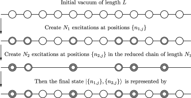
Figure 16: Nesting procedure for $su(3)$. In our example, $K=3$, $L=12$, $\{n_{1,j}\}=\{1,2,5,8,9,11\}$ and $\{n_{2,j}\}=\{1,3,4,5,6\}$. The final result reads $|2,1,0,0,2,0,0,1,2,0,2,0\rangle$, where $0$ denotes the vacuum state, $1$ denotes the first excited state and $2$ denotes the second excited state. In our ket notation, it is written as $|\{1,2,5,8,9,11\},\{1,3,4,5,6\}\rangle$.

The beauty of this method is that at each step, the operation is simple and the same: to create one kind of excitation in a reduced spin chain of length $N_{a}$. Here we see the nested feature of this method.

The wave function $\psi(\mathbf{u}_{1},\cdots,\mathbf{u}_{K-1})$ is constructed by nested Bethe ansatz. It is given in terms of a series of wave functions $\psi_{a}$, $a=2,\cdots,K-1$.The Bethe wave function reads

$$\psi(\mathbf{u}_{1},\cdots,\mathbf{u}_{K-1})=\sum_{\mathrm{P}_{1}}A_{1}(\mathrm{P}_{1})\prod_{j=1}^{N_{1}}\left(\frac{u_{1,\mathrm{P}_{1,j}}+\frac{i}{2}}{u_{1,\mathrm{P}_{1,j}}-\frac{i}{2}}\right)\psi_{2}(\mathrm{P}_{1})\;,$$ (A.3)

where the wave functions $\psi_{a}$, $a=2,\cdots,K-1$ are given by

$$\psi_{a}(\mathrm{P}_{a-1})=\sum_{\mathrm{P}_{a}}A_{a}(\mathrm{P}_{a})\prod_{j=1}^{N_{a}}\prod_{k=1}^{n_{a,j}}\frac{\left(u_{a,\mathrm{P}_{a,j}}-u_{a-1,\mathrm{P}_{a-1,k}}-M_{a-1,a}\frac{i}{2}\right)^{\delta_{k\neq n_{a,j}}}}{u_{a,\mathrm{P}_{a,j}}-u_{a-1,\mathrm{P}_{a-1,k}}+M_{a-1,a}\frac{i}{2}}\psi_{a+1}(\mathrm{P}_{a}).$$ (A.4)

with $\mathrm{P}_{a}$ the permutation $(P_{a,1},\ldots,P_{a,N_{a}})$ of $(1,\cdots,N_{a})$. We define $\psi_{K}(\mathrm{P}_{K-1})=1$. $M_{a,b}$ is the Cartan matrix of the Lie algebra, for $\mathfrak{su}(K)$ being

$$M_{a,b}=2\delta_{a,b}-\delta_{a-1,b}-\delta_{a+1,b}\;.$$ (A.5)

Our choice of normalization is

$$A_{a}(1,2\cdots,N_{a})=1$$ (A.6)

and the coefficients $A_{a}$ obey the relation

$$\frac{A_{a}(\cdots,i,j,\cdots)}{A_{a}(\cdots,j,i,\cdots)}=S_{2}(u_{a,i},u_{a,j})\;.$$ (A.7)

Here we used the following definition,

$$S_{\sigma}(u_{a,i},u_{b,j})=\frac{u_{a,i}-u_{b,j}+\frac{i}{2}\sigma}{u_{a,i}-u_{b,j}-\frac{i}{2}\sigma}\;,\qquad\sigma=1,2\;.$$ (A.8)

In order that (A.2) is an eigenstate of the spin chain Hamiltonian, the rapidities should satisfy the Bethe ansatz equations :

$$\left(\frac{u_{a,j}+V_{a}\frac{i}{2}}{u_{a,j}-V_{a}\frac{i}{2}}\right)^{L}=\prod_{b=1}^{r}\prod_{k=1\atop(a,j)\neq(b,k)}^{N_{b}}\frac{u_{a,j}-u_{b,k}+\frac{i}{2}M_{a,b}}{u_{a,j}-u_{b,k}-\frac{i}{2}M_{a,b}}\;,$$ (A.9)

where $V_{a}$ are the Dynkin labels. We consider the fundamental representation in this paper, where $V_{a}=\delta_{a,1}$.

Appendix B The $su(3)$ tailoring prescription

We consider the operators in $su(3)$ sector with definite one-loop anomalous dimensions. In the spin chain language, these operators are represented by the Bethe eigenstates of the $su(3)$ spin chain. One first write the Bethe state as the entangled state of two subchain states. This operation is called “cutting”. After cutting operation, each subchain state also takes the form of Bethe states. In order to perform Wick contraction, one needs to “flip” one of the subchains. Flipping is an operation that takes a ket state into the corresponding bra state with the same wave function. One can flip either the left or the right subchain. In this paper, we always flip the right subchain. The last step is to calculate the scalar product of Bethe states, this is called the “gluing” operation.

Consider a generic $su(2)$ Bethe state $|\mathbf{u}\rangle$ of a spin chain with length $L$. We define the first $l$ sites from the left to be the left subchain and the rest $L-l$ sites to be the right subchain. $|\mathbf{u}\rangle$ can be written as an entangled state of the subchains

$$|\mathbf{u}\rangle=\sum_{k=0}^{\text{min}\{N,l\}}\sum_{1\leq n_{1}<\cdots<n_{k}\leq l}\ \sum_{l\leq n_{k+1}<\cdots\leq L}\psi(\mathbf{u})|n_{1},\cdots,n_{k}\rangle_{\,l}\otimes|n_{k+1}-l,\cdots,n_{N}-l\rangle_{\,r}$$ (B.1)

where $k$ is the number of magnons in the left subchain. Note that one needs to re-label the positions of the magnons in the right subchain, see Fig.(17).

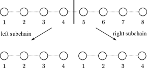
Figure 17: The cutting process for a spin chain with $L=8$. We take $l=4$ and $L-l=4$. The sites in the right subchain are originally labeled by $5,6,7,8$ while after cutting they are labeled by $1,2,3,4$.

Since we have two subchains, the magnons can either be in the left subchain or in the right subchain. After cutting a Bethe eigenstate, the resulting two subchains states still take the form of Bethe state. Hence the two subchain states have their own Bethe wave functions $\psi_{l}(\mathbf{u}^{\prime})$ and $\psi_{r}(\mathbf{u}^{\prime\prime})$, where $\mathbf{u^{\prime}}$ and $\mathbf{u^{\prime\prime}}$ is a partition of $\mathbf{u}$,

$$\mathbf{u}^{\prime}\cup\mathbf{u}^{\prime\prime}=\mathbf{u},\quad\mathbf{u}^{\prime}\cap\mathbf{u}^{\prime\prime}=\emptyset\;.$$ (B.2)

In general, $\psi(\mathbf{u})=H(\mathbf{u}^{\prime},\mathbf{u}^{\prime\prime})\;\psi_{l}(\mathbf{u}^{\prime})\,\psi_{r}(\mathbf{u}^{\prime\prime})$ where $H(\mathbf{u}^{\prime},\mathbf{u}^{\prime\prime})$ is a partition-dependent factor which shall be called $H$-factor from now on. Formally, the cutting of a Bethe state can be written as

$$|\mathbf{u}\rangle=\sum_{\alpha}H(\mathbf{u}^{\prime},\mathbf{u}^{\prime\prime})\,|\mathbf{u}^{\prime}\rangle\otimes|\mathbf{u}^{\prime\prime}\rangle\;.$$ (B.3)

Usually the expression for the $H$-factor is long. In order to make the expression more compact, we introduce some short-hand notations. Given a function $F(x,y)$ and two sets of variables $\mathbf{u}$, $\mathbf{v}$, we define

$$F(\mathbf{u},\mathbf{v})\equiv\prod_{u_{i}\in\mathbf{u},\;v_{j}\in\mathbf{v}}F(u_{i},v_{j}),\quad F^{>}(\mathbf{u},\mathbf{v})\equiv\prod_{i>j\atop u_{i}\in\mathbf{u},\;v_{j}\in\mathbf{v}}F(u_{i},v_{j})\;.$$ (B.4)

For a constant $c$, we define

$$F(\mathbf{u},c)=\prod_{u_{i}\in\mathbf{u}}F(u_{i},c),\quad F(c,\mathbf{v})=\prod_{v_{i}\in\mathbf{v}}F(c,v_{i})\;.$$ (B.5)

With the notations from (A.8) the $H$-factor for the $su(2)$ spin chain is given by

$$H(\mathbf{u}^{\prime},\mathbf{u}^{\prime\prime})=S_{1}(\mathbf{u}^{\prime\prime},0)^{l}\;S_{2}^{>}(\mathbf{u}^{\prime},\mathbf{u}^{\prime\prime})\;.$$ (B.6)

The cutting operation can be generalized to $su(K)$ Bethe state. Let us denote the nested Bethe state by $|{\mathbf{u}}\rangle$ where $\mathbf{u}=(\mathbf{u}_{1},\cdots,\mathbf{u}_{K-1})$. We have

$$|{\mathbf{u}}\rangle=\sum_{{\mathbf{u}}^{\prime}}H({\mathbf{u}}^{\prime},{\mathbf{u}}^{\prime\prime})\;|{\mathbf{u}}^{\prime}\rangle\otimes|{\mathbf{u}}^{\prime\prime}\rangle$$ (B.7)

with the $H$-factor

$$H({\mathbf{u}}^{\prime},{\mathbf{u}}^{\prime\prime})=\prod_{n=1}^{K-1}S_{1}(\mathbf{u}^{\prime\prime}_{n},\mathbf{u}^{\prime}_{n-1})\;S_{2}^{>}(\mathbf{u}^{\prime}_{n},\mathbf{u}^{\prime\prime}_{n})$$ (B.8)

where $\mathbf{u}^{\prime}_{0}$ is defined as $\mathbf{u}^{\prime}_{0}=\{0^{l}\}$ with $l$ the length of left subchain. In order to perform Wick contraction, we need to “flip” the right subchain from a ket state into a bra state. The flipping operation is different from Hermitian conjugate. Given a state

$$|\psi\rangle=e^{i\theta}|XZXZZ\rangle$$ (B.9)

the Hermitian conjugate and flipping (denoted by superscript $\mathcal{F}$) lead to

$$(|\psi\rangle)^{\dagger} =e^{-i\theta}\langle XZXZZ|$$

$$(|\psi\rangle)^{\mathcal{F}} =e^{+i\theta}\langle\bar{Z}\bar{Z}\bar{X}\bar{Z}\bar{X}|\;.$$

For an $su(2)$ Bethe state $|\mathbf{u}\rangle$, the flipped state is proportional to the hermitian conjugate of the Bethe state $|\mathbf{u}^{*}\rangle$

$$(|\mathbf{u}\rangle)^{\mathcal{F}}=\langle\mathbf{u}^{*}|F(\mathbf{u})$$ (B.10)

where $\mathbf{u}^{*}$ is the complex conjugate of $\mathbf{u}$ and we call the proportionality $F(\mathbf{u})$ the $F$-factor. For an $su(2)$ Bethe state, the $F$-factor reads

$$F(\mathbf{u})=S_{1}(\mathbf{u},0)^{L+1}\;S_{2}^{>}(\mathbf{u},\mathbf{u})$$ (B.11)

where $L$ is the length of the spin chain. For an $su(K)$ Bethe state $|\vec{\mathbf{u}}\rangle$, the $F$-factor is given by

$$F({\mathbf{u}})=\prod_{n=1}^{K-1}S_{1}(\mathbf{u}_{n},\mathbf{u}_{n-1})S_{2}^{>}(\mathbf{u}_{n},\mathbf{u}_{n})$$ (B.12)

where $\mathbf{u}_{0}$ is defined by $\mathbf{u}_{0}=\{0^{L+1}\}$. From now on, by “tailor” (denoted by $\mathcal{T}$) a (nested) Bethe state, we mean first cut the state and then flip the right subchain state. We define the product of the corresponding $H$-factor and the $F$-factor to be the $\mathrm{H}_{F}$ factor. For an $su(K)$ Bethe state $|\mathbf{u}_{1},\cdots,\mathbf{u}_{K-1}\rangle$

$$(|{\mathbf{u}}\rangle)^{\mathcal{T}}=\sum_{{\mathbf{u}}^{\prime}}\mathrm{H}_{F}^{\mathbf{u}}\;|{\mathbf{u}}^{\prime}\rangle\otimes\langle{\mathbf{u}}^{\prime\prime*}|$$ (B.13)

where

$${\mathbf{u}}^{\prime}\cup{\mathbf{u}}^{\prime\prime}={\mathbf{u}},\quad{\mathbf{u}}^{\prime}\cap{\mathbf{u}}^{\prime\prime}=\emptyset$$ (B.14)

and the $H_{F}$-factor reads

$$\mathrm{H}_{F}^{\mathbf{u}}=\prod_{n=1}^{K-1}S_{1}(\mathbf{u}^{\prime\prime}_{n},\mathbf{u}_{n-1})S_{2}^{>}(\mathbf{u}_{n},\mathbf{u}^{\prime\prime}_{n})\;.$$ (B.15)

Appendix C The functionals ${\mathscr{A}}^{\pm}$

C.1 Definition

For any set of points ${{\bf u}}=\{u_{j}\}_{j=1}^{N}$ in the complex plane and for any complex function $f(z)$, we define the pair of functionals ${\mathscr{A}}^{\pm}_{{\bf u}}[f]$, which are completely symmetric polynomials of degree $N$ of the variables $f(u_{1}),\dots,f(u_{N})$. The functional ${\mathscr{A}}^{\pm}_{{\bf u}}$ is defined as a sum of monomials labeled by all possible partitions of the set ${{\bf u}}$ into two disjoint subsets ${{\bf u}}^{\prime}$ and ${{\bf u}}^{\prime\prime}$, with ${{\bf u}}^{\prime}\cup{{\bf u}}^{\prime\prime}={{\bf u}}$,

$${\mathscr{A}}_{{{\bf u}}}^{\pm}[f] = \sum_{{{\bf u}}^{\prime}\cup{{\bf u}}^{\prime\prime}={{\bf u}}}\ \ \prod_{u^{\prime}\in{{\bf u}}^{\prime}}[-f(u^{\prime})]\prod_{u^{\prime\prime}\in{{\bf u}}^{\prime\prime}}{u^{\prime}-u^{\prime\prime}\pm i\over u^{\prime}-u^{\prime\prime}}.$$ (C.1)

The expansion (C.1) was thoroughly studied by Gromov, Sever and Vieira [29]. The expansion (C.1) is summed up by the following operator expression,

$${\mathscr{A}}^{\pm}_{{\bf u}}[f]=\hat{\mathscr{A}}^{\pm}_{{\bf u}}[f]\cdot 1\,,$$ (C.2)

where the different operator $\hat{\mathscr{A}}^{\pm}[{{\bf u}}]$ is defined as

$$\begin{aligned} \hat{\mathscr{A}}^{\pm}_{{\bf u}}[f]&\stackrel{{\scriptstyle\text{def}}}{{=}}{1\over\Delta_{{{\bf u}}}}\prod_{j=1}^{N}\left(1-f(u_{j})\,e^{\pm i\partial/\partial u_{j}}\right)\Delta_{{{\bf u}}},\qquad\Delta_{{{\bf u}}}=\sum_{j<k}(u_{j}-u_{k}).\end{aligned}$$ (C.3)

The operator functional $\hat{\mathscr{A}}^{\pm}[{{\bf u}}]$ is formally obtained from the c-functional ${\mathscr{A}}^{\pm}[{{\bf u}}]$ as

$$\hat{\mathscr{A}}^{\pm}_{{\bf u}}[f]={\mathscr{A}}^{\pm}_{{\bf u}}[f\,e^{i\partial}]\,.\$$ (C.4)

C.2 Properties

It was found in [29] that for constant function $f(u)=\kappa$, the expansion (C.1) does not depend on the positions of the rapidities ${{\bf u}}$ and the functional ${\mathscr{A}}^{\pm}_{{\bf u}}[f]$ is given in this case by

$${\mathscr{A}}^{\pm}_{{{\bf u}}}[\kappa]=(1-\kappa)^{N}.$$ (C.5)

The functional ${\mathscr{A}}^{\pm}[f]$ have other remarkable properties [32, 31]:

1) Determinant formula, Eq. (5.11), which is obtained by substituting $\Delta_{{\bf u}}=\det_{jk}(u_{j}^{k-1})$ in the definition (C.3).

2) Functional relations between ${\mathscr{A}}^{+}$ and ${\mathscr{A}}^{-}$:

$${\mathscr{A}}^{\mp}_{{{\bf u}}}[f] = {\mathscr{A}}^{\pm}_{{{\bf u}}}[1/f]\ \prod_{j=1}^{N}[-f(u_{j})]\,,$$ (C.6)

$${\mathscr{A}}^{\mp}_{{{\bf u}}}[f] = {\mathscr{A}}^{\pm}_{{\bf u}}\big{[}-{Q^{\mp\mp}_{{\bf u}}\over Q^{\pm\pm}_{{\bf u}}}\,f\big{]}\,.$$ (C.7)

3) Reduction formula:

$${\mathscr{A}}^{\pm}_{{{\bf u}}\cup{{\bf z}}}[f{Q_{{\bf z}}\over Q^{\pm\pm}_{{\bf z}}}]={\mathscr{A}}^{\pm}_{{\bf u}}[f]\,.$$ (C.8)

4) Factorization property:

$$\hat{\mathscr{A}}_{{{\bf u}}\cup{\bf v}}^{\pm}[f]=\hat{\mathscr{A}}_{{\bf u}}^{\pm}[{Q_{\bf v}^{\pm\pm}\over Q_{\bf v}}\,f]\cdot\hat{\mathscr{A}}_{\bf v}^{\pm}[{Q^{\pm\pm}_{{\bf u}}\over Q_{{\bf u}}}\,f]\,.$$ (C.9)

Aplying $N$ times the factorisation property, one obtains the representation

$$\hat{\mathscr{A}}^{\pm}_{{\bf u}}[f] = \prod_{j=1}^{N}\left(1-\,E^{\pm}_{j}f(u_{j})\ e^{i\partial/\partial u_{j}}\right),\qquad E^{\pm}_{j}=\underset{u\to u_{j}}{\text{Res}}{Q^{\pm\pm}_{{\bf u}}(u)\over Q_{{\bf u}}}.$$ (C.10)

Relation to the Slavnov determinant. The determinant of the kernel $\Omega(u,v)$ defined as

$$\Omega_{f}(u,v)=t(u-v)-{Q^{++}_{{\bf u}}\over Q^{--}_{{\bf u}}}(u)\,f(v)\,t(-u+v),$$ (C.11)

where the set ${{\bf u}}$ satisfies the “on-shell” condition

$$\quad{Q^{++}_{{\bf u}}(u_{j})\over Q^{--}_{{\bf u}}(u_{j})}\ f(u_{j})=-1\quad\text{for}\ u_{j}\in{{\bf u}},$$ (C.12)

is evaluated as [37]

$${\det_{jk}\Omega_{f}(u_{j},v_{k})\over\det_{jk}{1\over u_{j}-v_{k}+i}}={\mathscr{A}}^{+}_{{{\bf u}}\cup{\bf v}}[f].$$ (C.13)

C.3 Classical limit.

In the classical limit, the Bethe roots condensate in one or several disjoint cuts. Let ${\mathcal{C}}_{k}$ be a contour encircling the $k$-th cut anticloskwise and leaving outside all other singularities of $f$ and $G_{{\bf u}}$. The filling fraction of the $k$-th cut is

$$\alpha_{k}={1\over 2\pi L}\oint\limits_{{\mathcal{C}}_{k}}G_{{\bf u}}(u)du.$$ (C.14)

We consider the limit $L\to\infty$ with all $\alpha_{k}$ finite. Then the leading, linear in $L$, term of $\log{\mathscr{A}}^{\pm}$ is given by the contour integral

$$\log{\mathscr{A}}^{\pm}_{{\bf u}}[f] \simeq \pm\oint\limits_{{\mathcal{C}}_{{\bf u}}}\frac{du}{2\pi}\ \text{Li}_{2}\big{(}f(u)\,e^{\pm iG_{{\bf u}}(u)}\big{)}\,,\quad{\mathcal{C}}_{{\bf u}}=\cup_{k=1}^{n}{\mathcal{C}}_{k}.$$ (C.15)

While there is not yet a rigorous proof of this formula, it has passed a number of analytical and numerical checks. A heuristic derivation of (C.15) for $f(u)=\left({u-i/2\over u+i/2}\right)^{L}$, was presented in [29]. When $f(u)=\kappa$, it was shown in [29] that the quasiclassical formula (C.15) gives the exact answer (C.5). Moreover, the integral (C.15) satisfies the functional equation (C.6) thanks to the functional equation for the dilogarithm,

$$\text{Li}_{2}({1\over\omega})=-\text{Li}_{2}(\omega)-{\pi^{2}\over 6}-{1\over 2}\log^{2}(-\omega).$$ (C.16)

References

- [1] S. Lee, S. Minwalla, M. Rangamani, and N. Seiberg, “Three-Point Functions of Chiral Operators in D=4, =4 SYM at Large N,” ArXiv High Energy Physics - Theory e-prints (June, 1998) arXiv:hep-th/9806074.
- [2] D. Z. Freedman, S. D. Mathur, A. Matusis, and L. Rastelli, “Correlation functions in the CFTd/AdSd+1 correspondence,” Nuclear Physics B 546 (Apr., 1999) 96–118, arXiv:hep-th/9804058.
- [3] J. A. Minahan and K. Zarembo, “The Bethe-ansatz for N = 4 super Yang-Mills,” JHEP 03 (2003) 013, hep-th/0212208.
- [4] N. Beisert et al, “Review of AdS/CFT Integrability: An Overview,” Letters in Mathematical Physics 99 (Jan., 2012) 3–32, 1012.3982.
- [5] D. Serban, “Integrability and the AdS/CFT correspondence,” J. Phys. A: Math. Theor. 44 (2011) 124001, 1003.4214.
- [6] K. Okuyama and L.-S. Tseng, “Three-Point Functions in N=4 SYM Theory at One-Loop,” JHEP 8 (Aug., 2004) 55, arXiv:hep-th/0404190.
- [7] R. Roiban and A. Volovich, “Yang-Mills Correlation Functions from Integrable Spin Chains,” JHEP 9 (Sept., 2004) 32, arXiv:hep-th/0407140.
- [8] L. D. Faddeev, E. K. Sklyanin, and L. A. Takhtajan, “The Quantum Inverse Problem Method. 1,” Theor. Math. Phys. 40 (1979), no. 2, 688–706.
- [9] J. Escobedo, N. Gromov, A. Sever, and P. Vieira, “Tailoring three-point functions and integrability,” JHEP 9 (Sept., 2011) 28, 1012.2475.
- [10] O. Foda, “N= 4 SYM structure constants as determinants,” JHEP 3 (Mar., 2012) 96, 1111.4663.
- [11] N. Beisert, J. A. Minahan, M. Staudacher, and K. Zarembo, “Stringing spins and spinning strings,” JHEP 09 (2003) 010, hep-th/0306139.
- [12] V. Kazakov, A. Marshakov, J. A. Minahan, and K. Zarembo, “Classical / quantum integrability in AdS/CFT,” JHEP 05 (2004) 024, hep-th/0402207.
- [13] N. Beisert, V. Kazakov, K. Sakai, and K. Zarembo, “The algebraic curve of classical superstrings on AdS ,” Commun. Math. Phys. 263 (2006) 659–710, hep-th/0502226.
- [14] S. Schafer-Nameki, “Review of AdS/CFT Integrability, Chapter II.4: The Spectral Curve,” 1012.3989.
- [15] R. A. Janik, P. Surowka, and A. Wereszczynski, “On correlation functions of operators dual to classical spinning string states,” 1002.4613.
- [16] K. Zarembo, “Holographic three-point functions of semiclassical states,” Journal of High Energy Physics 9 (Sept., 2010) 30, 1008.1059.
- [17] E. Buchbinder and A. Tseytlin, “On semiclassical approximation for correlators of closed string vertex operators in AdS/CFT,” JHEP 1008 (2010) 057, 1005.4516.
- [18] R. A. Janik and A. Wereszczynski, “Correlation functions of three heavy operators - the AdS contribution,” ArXiv e-prints (Sept., 2011) 1109.6262.
- [19] E. I. Buchbinder and A. A. Tseytlin, “Semiclassical correlators of three states with large charges in string theory in AdS5xS5,” Phys. Rev. D 85 (Jan., 2012) 026001, 1110.5621.
- [20] T. Klose and T. McLoughlin, “A light-cone approach to three-point functions in AdS_5 x S^5,” ArXiv e-prints (June, 2011) 1106.0495.
- [21] Y. Kazama and S. Komatsu, “On holographic three point functions for GKP strings from integrability,” ArXiv e-prints (Oct., 2011) 1110.3949.
- [22] Y. Kazama and S. Komatsu, “Wave functions and correlation functions for GKP strings from integrability,” ArXiv e-prints (May, 2012) 1205.6060.
- [23] M. S. Costa, R. Monteiro, J. E. Santos, and D. Zoakos, “On three-point correlation functions in the gauge/gravity duality,” JHEP 1011 (2010) 141, 1008.1070.
- [24] R. Roiban and A. Tseytlin, “On semiclassical computation of 3-point functions of closed string vertex operators in AdS,” 1008.4921.
- [25] J. Escobedo, N. Gromov, A. Sever, and P. Vieira, “Tailoring Three-Point Functions and Integrability II. Weak/strong coupling match,” 1104.5501.
- [26] J. Caetano and J. Escobedo, “On four-point functions and integrability in N=4 SYM: from weak to strong coupling,” ArXiv e-prints (July, 2011) 1107.5580.
- [27] G. Georgiou, “SL(2) sector: weak/strong coupling agreement of three-point correlators,” Journal of High Energy Physics 9 (Sept., 2011) 132, 1107.1850.
- [28] S. Frolov and A. A. Tseytlin, “Rotating string solutions: AdS/CFT duality in non-supersymmetric sectors,” Physics Letters B 570 (Sept., 2003) 96–104, arXiv:hep-th/0306143.
- [29] N. Gromov, A. Sever, and P. Vieira, “Tailoring Three-Point Functions and Integrability III. Classical Tunneling,” ArXiv e-prints (Nov., 2011) 1111.2349.
- [30] V. E. Korepin, “Calculation of norms of Bethe wave functions,” Communications in Mathematical Physics 86 (1982) 391–418. 10.1007/BF01212176.
- [31] I. Kostov, “Three-point function of semiclassical states at weak coupling,” ArXiv e-prints (May, 2012) 1205.4412.
- [32] I. Kostov, “Classical Limit of the Three-Point Function of N=4 Supersymmetric Yang-Mills Theory from Integrability,” Physical Review Letters 108 (June, 2012) 261604, 1203.6180.
- [33] N. Gromov and P. Vieira, “Quantum Integrability for Three-Point Functions,” ArXiv e-prints (Feb., 2012) 1202.4103.
- [34] D. Serban, “A note on the eigenvectors of long-range spin chains and their scalar products,” ArXiv e-prints (Mar., 2012) 1203.5842.
- [35] N. Gromov and P. Vieira, “Tailoring Three-Point Functions and Integrability IV. Theta-morphism,” ArXiv e-prints (May, 2012) 1205.5288.
- [36] M. Wheeler, “Scalar products in generalized models with SU(3)-symmetry,” ArXiv e-prints (Apr., 2012) 1204.2089.
- [37] I. Kostov and Y. Matsuo, “Inner products of Bethe states as partial domain wall partition functions,” JHEP10(2012)168 (July, 2012) 1207.2562.
- [38] V. E. Korepin, “Norm of Bethe Wave Function as a Determinant,” ArXiv e-prints (Nov., 2009) 0911.1881.
- [39] N. Reshetikhin, “Calculation of the norm of bethe vectors in models with SU(3)-symmetry,” Zap. Nauchn. Semin. LOMI 150 (1986) 196–213.
- [40] N. A. Slavnov, “On Scalar Products in the Algebraic Bethe Ansatz,” Tr. Mat. Inst. Steklova 251 (2005) 257–264.
- [41] N. A. Slavnov, “The algebraic Bethe ansatz and quantum integrable systems,” Russian Mathematical Surveys 62 (2007), no. 4, 727.
- [42] N. Gromov and P. Vieira, “Complete 1-loop test of AdS/CFT,” JHEP 4 (Apr., 2008) 46, 0709.3487.
- [43] J. Caetano and P. Vieira, private communication. See also ref. [13] of [36].
- [44] S. Belliard, S. Pakuliak, E. Ragoucy, and N. A. Slavnov, “Algebraic Bethe ansatz for scalar products in SU(3)-invariant integrable models,” ArXiv e-prints (July, 2012) 1207.0956.
- [45] N. Beisert, V. Kazakov, K. Sakai, and K. Zarembo, “Complete spectrum of long operators in N = 4 SYM at one loop,” JHEP 07 (2005) 030, hep-th/0503200.
- [46] B. Sutherland, “Low-Lying Eigenstates of the One-Dimensional Heisenberg Ferromagnet for any Magnetization and Momentum,” Phys. Rev. Lett. 74 (Jan, 1995) 816–819.
- [47] A. Dhar and B. Sriram Shastry, “Bloch Walls and Macroscopic String States in Bethe’s Solution of the Heisenberg Ferromagnetic Linear Chain,” Phys. Rev. Lett. 85 (Sep, 2000) 2813–2816.
- [48] M. Takahashi, “One-Dimensional Hubbard Model at Finite Temperature,” Progress of Theoretical Physics 47 (1972), no. 1, 69–82.
- [49] N. Beisert, V. Kazakov, and K. Sakai, “Algebraic curve for the SO(6) sector of AdS/CFT,” Commun. Math. Phys. 263 (2006) 611–657, hep-th/0410253.
- [50] C. Kristjansen, “Three-spin strings on AdS(5) x S**5 from N = 4 SYM,” Phys. Lett. B586 (2004) 106–116, hep-th/0402033.
- [51] M. Kruczenski, “Spin chains and string theory,” Phys.Rev.Lett. 93 (2004) 161602, hep-th/0311203.
- [52] A. Bissi, T. Harmark, and M. Orselli, “Holographic 3-Point Function at One Loop,” JHEP 1202 (2012) 133, 1112.5075.
- [53] R. A. Janik and P. Laskos-Grabowski, “Surprises in the AdS algebraic curve constructions - Wilson loops and correlation functions,” ArXiv e-prints (Mar., 2012) 1203.4246.
- [54] D. Correa, J. Maldacena, and A. Sever, “The quark anti-quark potential and the cusp anomalous dimension from a TBA equation,” ArXiv e-prints (Mar., 2012) 1203.1913.
- [55] N. Drukker, “Integrable Wilson loops,” ArXiv e-prints (Mar., 2012) 1203.1617.
- [56] A. Sever, P. Vieira, and T. Wang, “From Polygon Wilson Loops to Spin Chains and Back,” ArXiv e-prints (Aug., 2012) 1208.0841.
- [57] N. Gromov and A. Sever, “Analytic Solution of Bremsstrahlung TBA,” ArXiv e-prints (July, 2012) 1207.5489.
- [58] J. Caetano and J. Toledo, “-Systems for Correlation Functions,” 1208.4548.
- [59] M. S. Costa, V. Goncalves, and J. Penedones, “Conformal Regge theory,” Journal of High Energy Physics 12 (Dec., 2012) 91, 1209.4355.
- [60] V. Kazakov and E. Sobko, “Three-point correlators of twist-2 operators in N=4 SYM at Born approximation,” ArXiv e-prints (Dec., 2012) 1212.6563.
- [61] J. Plefka and K. Wiegandt, “Three-Point Functions of Twist-Two Operators in N=4 SYM at One Loop,” JHEP 1210 (2012) 177, 1207.4784.
- [62] B. Eden, “Three-loop universal structure constants in N=4 susy Yang-Mills theory,” ArXiv e-prints (July, 2012) 1207.3112.
- [63] J. Escobedo, Integrability in AdS/CFT: Exact Results for Correlation Functions. PhD thesis, University of Waterloo, 2012.