Synchronization, quantum correlations and entanglement in oscillator networks

Abstract

Synchronization is one of the paradigmatic phenomena in the study of complex systems. It has been explored theoretically and experimentally mostly to understand natural phenomena, but also in view of technological applications. Although several mechanisms and conditions for synchronous behavior in spatially extended systems and networks have been identified, the emergence of this phenomenon has been largely unexplored in quantum systems until very recently. Here we discuss synchronization in quantum networks of different harmonic oscillators relaxing towards a stationary state, being essential the form of dissipation. By local tuning of one of the oscillators, we establish the conditions for synchronous dynamics, in the whole network or in a motif. Beyond the classical regime we show that synchronization between (even unlinked) nodes witnesses the presence of quantum correlations and entanglement. Furthermore, synchronization and entanglement can be induced between two different oscillators if properly linked to a random network.

*Correspondence to roberta@ifisc.uib-csic.es

Synchronization is a paradigmatic and well studied phenomenon in many biological, physical and social systems Strogatz ; Pikovsky ; Arenas , also proposed as a tool in view of applications Athen , but almost unexplored in the quantum regime. Interesting exceptions entrain1 ; entrain2 ; entrain3 deal with entrainment, i.e. synchronization as the response to an external driver. At the microscopic level, spontaneous synchronization was recently predicted in nanomechanical oscillators Marquardt2011 ; Milburn2011 and observed Lipson2012 in the classical regime, when quantum fluctuations are neglected. Indeed a first approximation to a great variety of quantum systems, such as electromagnetic modes opt1 ; opt2 ; opt3 , trapped ions ions1 ; ions2 or nanoelectromechanical resonators Plenio , is given by a set of coupled quantum harmonic oscillators, susceptible to experience spontaneous synchronization. Beyond physical systems, there is an increasing awareness that quantum phenomena might play an important role in terms of efficiency of biological processes. Several examples Gauger2011 ; Panitchayangkoon ; Engel have shown that we may have to consider quantum dynamics to explain biological phenomena.

A first step to characterize quantum spontaneous synchronization, considering quantum fluctuations and correlations beyond the classical limit, has been taken in Ref.PRAsync where synchronization between one pair of damped quantum harmonic oscillators has been reported. Most of the classical literature deals with self-sustained phase oscillators modeled by Kuramoto-type models, or with identical nonlinear oscillators studied through the master stability formalism Arenas . Ref. PRAsync takes a different view focusing on synchronization during the relaxation dynamics of different linear oscillators driven out of equilibrium and exploring the key role of dissipation. Indeed, depending on the way in which damping occurs, a pair of oscillators with different frequencies can show synchronous evolution emerging after a transient, as well as robust (slowly decaying) non-classical correlations PRAsync . When several dissipative quantum oscillators coupled in a network are considered dissipation can act globally or locally (in a node) and, depending on the correlation length in the bath with respect to the size of the system, a variety of surprising phenomena are observed. In this work we show how synchronization can actually be induced by local tuning of one (even newly attached) oscillator of a generic (regular or random) network. Synchronous behavior emerges in the whole network or in a part of it and witnesses robust quantum correlations and entanglement. Stemming both from the structure of the system and from the form of system-bath coupling we further show the possibility to tune the system to configurations in which nodes do not thermalize and relax into a synchronous and non-classical asymptotic state.

The form in which dissipation occurs in a spatially extended system has deep consequences. We stress that the importance of symmetries present in the system-bath coupling has been recognized in many contexts. In classical systems, this fundamental issue was already discussed in the seminal work of Lord Rayleigh analyzing damping effects on normal modes in vibrating systems Rayleigh . Indeed, the role of dissipation to reduce detrimental effects of vibrations is fundamental in many areas of mechanical, civil and aerospace engineering Engineering . On the other hand, in the context of quantum systems, symmetries in the coupling between qubits and the environment allow for decoherence-free subspaces dfs , entangled states preparation Diehl ; Barreiro2010 and dissipative quantum computing cirac2009 ; blatt2011 .

In the following we show that the distribution and form of losses through the network amounts to synchronous dynamics in spite of the nodes diversity, and robust quantum correlations. Furthermore, steady entanglement can be generated between unlinked nodes by properly coupling them to a network.

Results

Dissipation mechanisms and synchronization

We consider generic networks of $N$ nonresonant, coupled quantum harmonic oscillators, given by the Hamiltonian

$$H_{S}=\frac{1}{2}\left(\bf{p}^{T}{\bf{p}}+{\bf{q}}^{T}\mathcal{H}{\bf{q}}\right)$$ (1)

where ${\bf{q}}^{T}=(q_{1},...,q_{N})$ is the vector of canonical position operators and ${\bf{p}}$ are momenta, satisfying $[q_{j},p_{j}]=i$ (we take $\hbar=1$ throughout the paper), and $\mathcal{H}_{m,n}=\omega_{m}^{2}\delta_{mn}+\lambda_{mn}(1-\delta_{mn})$ is the matrix containing the topological properties of the network (frequencies $\omega_{m}$ and couplings $\lambda_{mn}$). The eigenmodes of the system $\bf{Q}$ result from diagonalization of this Hamiltonian through the transformation matrix $\mathcal{F}$.

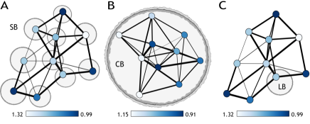
Figure 1: (A) Network of oscillators (represented by the network nodes) dissipating into separate baths (SB, represented by the gray circles surrounding the nodes). Links, representing couplings, have different strengths (lines thickness) and nodes have different natural frequencies (corresponding to different colors as given in the color bar). (B) Network of oscillators dissipating into a common bath (CB). (C) Network of oscillators with dissipation restricted to one node, local bath (LB).

Any realistic model needs to include also environment effects Weiss ; Schloss ; gardiner and, depending on system and bath correlations lengths, different forms of dissipation can be envisaged for an extended network (see Methods). All units can dissipate into separate identical baths (SB), Fig.1A, as cavity optical modes Weiss ; gardiner . Otherwise, if the coherence length of the environment is larger than the size of the system (here given by the spatial extension occupied by the oscillators network in Eq.(1)), all the nodes feel a ’similar’ dissipation. This common bath (CB), Fig.1B, is known to create decoherence-free subspaces dfs ; Viola and asymptotic entanglement klesse ; paz-roncaglia ; liu ; galve2010 . A third, limiting, case (LB) in which a specific oscillator $d$ dissipates much faster than any other node (Fig.1B) is also considered (local bath).

One of the key insights of our work comes from noting that the coupling of real oscillators to the bath (taken here to be equal, $\gamma$) differs from those of eigenmodes. The latter are found to be $\gamma\kappa_{m}$ (with $\kappa_{m}^{CB}=\sum_{n}\mathcal{F}_{nm}$, $\kappa_{m}^{SB}=1$ and $\kappa_{m}^{LB}=\mathcal{F}_{dm}$) meaning that, except the SB situation, the eigenmodes have different decay rates. Then for CB and LB only the least dissipative eigenmode will survive to thermalization, thus governing the motion of all oscillators overlapping with it. It is then useful identifying the less dissipating normal mode with smallest effective coupling, $\kappa_{\sigma}$, and also the following one, $\kappa_{\eta}$, such that $|\kappa_{\sigma}|\leq|\kappa_{\eta}|$. Further, in the case of an Ohmic bath with cut-off-frequency larger than the frequencies of the system, the normal-mode damping rates simplify to the form $\Gamma_{i}=\gamma~{}\kappa_{i}^{2}$

Conditions for synchronization in a network

Knowledge of the normal modes of a complex network and of their dissipation rates (or effective couplings) allows to fully characterize a large variety of phenomena. Indeed this is a simple but powerful approach, even if diagonalization of the problem needs to be performed numerically except in a few (highly symmetric) configurations. By the diagonalization matrix $\mathcal{F}$ and system-bath interaction Hamiltonian we obtain the conditions to have a dominating mode during a transient. This mode dissipating most slowly, $|\kappa_{\sigma}|<|\kappa_{j}|$ $\forall j\neq\sigma$, is found either for CB or LB. Even more important, it is possible to identify normal modes completely protected against dissipation, so that some network’s nodes do not thermalize. Indeed, a normal mode $\sigma$ is protected against decoherence if $\kappa_{\sigma}=0$. For a pair of oscillators interacting with a CB, this condition is accomplished only in the trivial case of identical frequencies paz-roncaglia ; galve2010 but this is not the case when more than two nodes are considered. We find that asymptotic synchronized quantum states can then be observed even in random networks where all nodes have different natural frequencies.

Full characterization of the quantum state evolution of the network comes from moments of all orders of the oscillator operators ${{q}_{j}}$ and ${{p}_{j}}$ gardiner . For SB, average positions (and momenta) are characterized by irregular oscillations before thermalization (Fig. 2A). On the other hand, for dissipation in CB and after a transient, regular phase locked oscillations can arise, as shown in Fig. 2B. Synchronization between detuned nodes can be found during a rather long and slow relaxation, like in the case of just one pair PRAsync . Further, the oscillations can remain robust even asymptotically if the condition $\kappa_{\sigma}=0$ is satisfied.

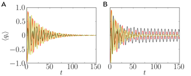
Figure 2: First order moments for initial conditions $-\langle q_{1}\rangle=\langle q_{3}\rangle=1.0$, $\langle q_{2}\rangle=0.0$, and vanishing momenta in the case of an open chain of three oscillators with $\omega_{1}=1.2~{}\omega_{2}$, $\omega_{3}=1.8~{}\omega_{2}$, non-vanishing couplings $\lambda_{12}=\lambda_{23}=0.4~{}\omega_{2}^{2}$, temperature $T=10~{}\omega_{2}$ (Boltzmann constant taken to be unity), $\gamma=0.07~{}\omega_{2}^{2}$, bath cutoff $50~{}\omega_{2}$, for SB (A) and for CB (B). Time is scaled in units of the inverse of the reference frequency $\omega_{2}$.

Beyond the classical limit given by average positions and momenta, let us now consider the full quantum dynamics stemming from the evolution of higher moments (see SI). At the microscopic level, quantum fluctuations also oscillate in time (even for initial vacuum states for which first order moments vanish at any time). This collective periodic motion is associated to a slow energy decay and witnesses the presence of robust quantum correlations against decoherence Schloss . Our approach points to a wide range of appealing possibilities in quantum networks. In the following we show how a whole random network (or a part of it) can be brought to a synchronized state retaining quantum correlations via local tuning of just one of the nodes, or how two external oscillators can be linked to a random network leading to their entanglement and locked oscillations.

Collective synchronization by tuning one oscillator

Let us consider an Erdös-Rényi random and dissipative network Arenas of oscillators with different node frequencies, links and weights (Fig. 1) focusing on the relaxation dynamics of energy and quantum correlations. The node dynamics is mostly incoherent and even if initializing the network in a non-classical state, quantum correlations generally disappear due to decoherence Schloss . Independently on the form of the network, for dissipation in SB, all nodes thermalize on a time scale $\gamma^{-1}$ (see Eq. (8) and Methods). As anticipated before, this is not the case in the presence of a dissipation acting not-uniformly within the network.

Common dissipation bath

In presence of CB, an arbitrary network of $N$ nodes can reach a synchronized state before thermalization if there is a weakest effective coupling $\kappa_{\sigma}$. As a matter of fact just by tuning one of the node frequencies, $\omega_{v}$, even maintaining fixed the rest of the network frequencies $\{\omega_{l\neq v}\}$ and its topology ($\lambda_{ij}$ couplings) it is possible to decrease the weakest coupling $\kappa_{\sigma}$. This means that an extra oscillator of properly selected frequency $\{\omega_{l\neq v}\}$ (like a synchronizer) can be added to a random network, even if weakly coupled, and it will lead to a collective synchronization of the whole system at some frequency ($\Omega_{\sigma}$), generally different from $\omega_{v}$. Fig. 3 displays the average global synchronization and quantum correlations established in the network. Synchronization arises after a transient across the whole network by tuning one of the frequencies $\omega_{v}$ to a particular value $\bar{\omega}_{v}$, while it is not present when moving a few percent away from this value. Equivalently one could have tuned one of the couplings $\lambda_{vv^{\prime}}$. In the following we consider separately the case in which $\kappa_{\sigma}$ is significantly smaller than the other effective couplings and the case in which it vanishes.

Conditions for global synchronization follow from small ratio between the damping rates of the two slowest normal modes $R=\kappa_{\sigma}/\kappa_{\eta}\rightarrow 0$. Interestingly, this is a necessary but not sufficient condition for $collective$ synchronization. This is due to the fact that the presence of a slowly dissipating normal mode into the system needs to be accompanied by a significant overlap between this mode ($Q_{\sigma}$), or virtual oscillator, and all the real ones ($q_{1},...,q_{N}$). An analytical estimation of the synchronization time is found taking into account both the importance (overlap with individual oscillator) and decay of few normal modes in the system. The time for oscillator $j$ to start oscillating at the less damped frequency $\Omega_{\sigma}$ reads:

$$t^{(j)}\equiv\max_{\{k\neq\sigma\}}2\frac{\log{\mathcal{F}_{jk}}-\log{\mathcal{F}_{j\sigma}}}{\Gamma_{k}-\Gamma_{\sigma}}\ ,$$ (2)

maximizing over all modes $k$ different from the slowest one $\sigma$ (see SI). Collective synchronization time corresponds to $t_{sync}=\max_{\{j\}}\{t^{(j)}\}$, i.e. when even the last oscillator joins the synchronous dynamics dominated by the less damped mode. Then phase-locking in the evolution of all oscillators, namely in their (all order) moments, can arise before thermalization, when there is significant separation between largest time decays $\Gamma_{\eta},\Gamma_{\sigma}$, and overlap between slowest normal modes and each system node. Global network synchronization (see Methods) obtained from the full dynamical evolution and the estimated synchronization time $t_{sync}$ are in good agreement, as seen in Fig. 3A. For the same network, the ratio $R$, the collective synchronization $\mathcal{S}$ and mean discord $\langle\delta\rangle$ at long times can be seen in Fig. S1 (see SI).

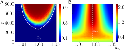
Figure 3: (A) Time evolution of synchronization $\mathcal{S}$, and (B) quantum correlations quantified by the discord $\langle\delta\rangle\times 10^{3}$ , when varying one node frequency $\omega_{v}$. Results are shown for a random network (connection probability $p=0.6$) of $10$ oscillators. Frequencies of nodes are sampled from a uniform distribution from $0.9\omega_{0}$ to $1.2\omega_{0}$ and couplings from a Gaussian distribution around $-0.1\omega_{0}^{2}$ with standard deviation $0.05\omega_{0}^{2}$. Environment parameters (here and in the following figures) are $\gamma=0.01\omega_{0}^{2}$, $T=10\omega_{0}$ and cut-off frequency $\Lambda=50\omega_{0}$ (see Methods). Time units are chosen so that $\omega_{0}=1$. Collective synchronization $\mathcal{S}$ and (averaged and filtered) discord $\delta$ (see Methods) are obtained considering all oscillator pairs of the network. Dashed line identifies the frequency $\bar{\omega}_{v}$ for which $\kappa_{\sigma}=0$. Continuous line in (A) corresponds to the estimated synchronization time $t_{sync}$.

We now look at the quantumness of the state in presence of collective synchronization. Generally decoherence is independent on the specific features such as the oscillation frequency in a system CaldeiraLeggett . Still, synchronization is a consequence of a reduced dissipation in some system mode and indeed witnesses the robustness of quantum correlations, as evident form the average discord $\langle\delta\rangle$ in the network represented in Fig.3B. After a transient dynamics in which the couplings in the network create quantum correlations Plenio , even when starting from separable states, discord does actually decay to small values for $\omega_{v}$ different from $\bar{\omega}_{v}$ (non-synchronized network) while it maintains large values for the case of a properly tuned node ($\omega_{v}\sim\bar{\omega}_{v}$).

The case $\omega_{v}=\bar{\omega}_{v}$, leading to $\kappa_{\sigma}=0$, needs special attention. After a transient all the nodes will oscillate at a locked common frequency, the one of the undamped normal mode $\Omega_{\sigma}$, which we call a frozen mode. As before (Eq.(2)), the possibility to synchronize the whole network also requires a second condition, namely that the undamped mode involves all the network nodes. (The case in which the latter condition applies only to some nodes is discussed below.) When both the conditions

$$\kappa_{\sigma}=\sum_{k=1}^{N}\mathcal{F}_{k\sigma}=0\text{ , and }\mathcal{F}_{k\sigma}\neq 0\text{ }\forall k$$ (3)

are met, there is a frozen normal mode linking all oscillators. This leads to collective synchronization in the whole network and allows for mutual information and quantum correlations remaining strong even asymptotically, being orders of magnitude larger than for the fully thermalized state, when synchronization is not present (Fig.3). The undamped mode gives actually rise to a decoherence-free dynamics for the whole system of oscillators where quantum correlations and mutual information survive.

The phenomena above are found for nodes dissipating at equal rates into a CB, while in the presence of $N$ independent environments (SB) all oscillators thermalize incoherently, synchronization is not found, and decoherence times for all oscillators are of the same order. As a final observation we mention the special case in which the center of mass of the system is one of the normal modes; then there will be a large decoherence-free subspace (corresponding to the other $N-1$ modes) but no synchronization will appear for a CB.

Local dissipation bath

Common and separate baths correspond to two extreme situations in which all oscillators have equivalent interactions with the environment(s). We now consider the case of a local bath, as a limit case in which one oscillator is dissipating stronger, Fig.1C. A frozen normal mode $\sigma$ must not overlap with the dissipative oscillator (labeled by $d$) while involving all the other nodes ($\mathcal{F}_{i\sigma}\neq 0$ $\forall~{}i\neq d$). Then, synchronization of the whole network (except for the dissipative oscillator) arises. This occurs when

$$\mathcal{F}_{d\sigma}=0\text{ , with }\mathcal{F}_{dj}\neq 0\text{ }\forall~{}j\neq\sigma$$ (4)

meaning that the undamped mode $\sigma$ involves a cluster of oscillators not including the lossy one. We find synchronization and robust quantum effects across the network as for CB, with the difference that for LB the dissipating node is now excluded (further details are discussed in SI).

Synchronization of linear motifs

The possibility to synchronize a whole network, in presence of different dissipation mechanisms, just by tuning one local parameter opens-up the perspective of control that can be explored considering the dynamical variation of a control-node frequency. In particular we find similar qualitative results both for random networks and for disordered lattices consisting of regular networks with inhomogeneous frequencies and couplings, being the latter largely studied in ultracold atomic gases lew . Local tuning to collective synchronization is not only a general feature of different kind of networks but can also be established in motifs within the network. As we show in the following, the system can be tuned to a partial synchronization, involving some nodes of a network independently of the rest of it. Indeed, even if the whole system is coupled to a CB, we can identify the conditions for having a synchronized cluster, like the 3-node linear motif in Fig. 4. Two non-directly linked nodes $a$ and $b$ of the motif are then asymptotically synchronized through another one, here $c$, and this leads to a common oscillation dynamics along the whole motif $a$-$c$-$b$. The condition for synchronization of a cluster, namely its dependence on a frozen normal mode, reads

$$\frac{\lambda_{ac}}{\Omega_{\sigma}^{2}-\omega_{a}^{2}}+\frac{\lambda_{bc}}{\Omega_{\sigma}^{2}-\omega_{b}^{2}}=-1$$ (5)

with $\Omega_{\sigma}$ frequency of the frozen mode (see details in SI).

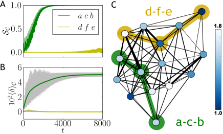
Figure 4: (A) Synchronization factors $\mathcal{S}_{C}$ and (B) average discord $\delta_{C}\times 10^{2}$ evaluated for linear 3-node motifs (hence the subindex $\mathcal{C}$) in a random network (connection probability $p=0.6$) of $15$ oscillators (shown in C). A tuned non-dissipative motif $\mathcal{C}_{1}$ composed by the three nodes $(a-c-b)$ is compared with another equivalent non-tuned motif $\mathcal{C}_{2}$ composed by nodes $(d-f-e)$. Frequencies in the network are sampled from a uniform distribution from $\omega_{0}$ to $1.8\omega_{0}$, and couplings with a Gaussian distribution around $-0.1\omega_{0}^{2}$ with standard deviation $0.05\omega_{0}^{2}$. In order to avoid dissipation in the $(a-c-b)$ motif we have set $\omega_{c}=1.51~{}\omega_{0}$, being $\lambda_{ac}=-0.09~{}\omega_{0}^{2}$ and $\lambda_{bc}=-0.11~{}\omega_{0}^{2}$. Time units such that $\omega_{0}=1$.

This case is an example of the general result stating that given any network, a part of it (in our case a linear motif, $\mathcal{C}_{1}$) can be synchronized by tuning one of its components, for instance a frequency or coupling of the motif. A key point is that this is independent of the frequencies and links of the rest of the network, provided the motif is properly embedded in the network. The links between $\mathcal{C}_{1}$ and the rest of the network should satisfy

$$\left(\frac{\lambda_{ac}}{\Omega_{s}^{2}-\omega_{a}^{2}}\right)\lambda_{aj}+\left(\frac{\lambda_{bc}}{\Omega_{s}^{2}-\omega_{b}^{2}}\right)\lambda_{bj}+\lambda_{cj}=0\ ,\ \forall j\ .$$ (6)

This is equivalent to saying that a synchronized motif with robust quantum correlations can preserve these features when linked to an $arbitrary$ network, if some constraints on the reciprocal links are satisfied. For instance, each node of the synchronized motif needs to share with the rest of the network more than one link. In Fig. 4 we compare the behavior of two linear motifs of a large network, where a first motif $\mathcal{C}_{1}$ is synchronized, satisfying Eqs.(5)-(6) while the second one $\mathcal{C}_{2}$ is not. After a transient a frozen mode tames the dynamics of $\mathcal{C}_{1}$, which then shows a synchronous evolution and robust correlations. It can also be shown that quantum purity and energy reach higher values of a stationary non-thermal state. This is compared with the non-synchronized motif $\mathcal{C}_{2}$ whose dynamics quickly relaxes to a thermal state. The case of a three oscillator chain is an example showing the possibility to tune synchronization and quantum effects in a motif within the network when the proper link conditions are satisfied.

Entangling two oscillators through a network

The same technique discussed in the previous section can be applied to the case in which we aim to synchronize few, even if not directly connected, elements of a network. But this does not mean that any set of nodes can be synchronized asymptotically. In fact, we find that for a CB we can only synchronize two different and not directly linked ($\lambda_{ab}=0$) oscillators if we synchronize with them also other intermediate linked elements (like in the linear motif example, Fig. 4) or when these two oscillators are identical, like we discuss in the present section.

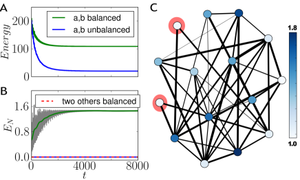
Figure 5: (A) Energy evolution and (B) entanglement (logarithmic negativity) between two nodes with identical frequency $\omega_{0}$ (we call these nodes $a$ and $b$ and are plotted in red in the network displayed in panel (C)). The network is a random one (connection probability $p=0.6$ of 15 oscillators and same frequency and couplings distribution as in Fig. 4. We compare the situations in which the couplings from the red nodes to the rest of the network (they are directly connected to other nodes called $c$ and $d$) are properly balanced in order to avoid dissipation $(\lambda_{ac}=\lambda_{bc}=-0.15\omega_{0}^{2}$ and $\lambda_{ad}=\lambda_{bd}=-0.12\omega_{0}^{2})$ with the case when this balance is perturbed $(\lambda_{ac}+0.04\omega_{0}^{2}$ and $\lambda_{ad}+0.04\omega_{0}^{2})$ .The third line in panel (B) shows the entanglement between other two arbitrary oscillators in the situation in which $a$ and $b$ are balanced. Time units such that $\omega_{0}=1$

We consider the case of two identical oscillators (i.e. with $\omega_{a}=\omega_{b}$) prepared in a separable state, with some local squeezing. They are not directly coupled ($\lambda_{ab}=0$) but are connected through an arbitrary network. In general they will dissipate reaching the thermal state, but with the proper conditions we find an important result: because their frequencies are identical it is possible to construct a frozen normal mode involving only these two nodes, given by $Q_{\sigma}=\mathcal{F}_{a\sigma}~{}q_{a}+\mathcal{F}_{b\sigma}~{}q_{b},$ with $\mathcal{F}_{a\sigma},\mathcal{F}_{b\sigma}\neq 0$ and this can be obtained, for instance, by properly attaching them to the network. In other words, by tuning their couplings to the network it is possible to have both oscillators relaxing onto a frozen mode, so that they will be synchronized and will keep a higher energy than otherwise. Most importantly, in this case entanglement can actually be generated between oscillators initially in a separable state and remains high asymptotically.

In order to entangle the oscillators, their coupling to the rest of the network needs to fulfill the condition

$$\sum_{k=a,b}\mathcal{F}_{k\sigma}\lambda_{kj}=0,$$ (7)

(similar to Eq. (6)), achieved by proper tuning of coupling strengths of the active links ($j$) with the rest of the network $\lambda_{aj},\lambda_{bj}$. In Fig. 5A and B we show the evolution of energy and entanglement of the oscillators $a$ and $b$ when linked to a random network. As we see in Fig. 5C there is not direct link between $a$ and $b$ ($\lambda_{ab}=0$) and the whole system dissipates in a common environment. The case where the oscillators $a$ and $b$ are coupled to the network following the prescription (7) is compared to another case in which their links are not properly balanced (we slightly change the coupling strengths). Both energy and entanglement are shown to be sensitive to the structure of the reciprocal links and the possibility to actually bring the added nodes into an entangled state that will survive asymptotically is guaranteed by Eq. (7). The importance of this result is twofold: in terms of applications it shows that it is possible to dynamically generate entanglement between two non-linked nodes embedded in a random network by tuning their connections to it, and on the other hand it enlarges the scenario for asymptotic entanglement generation through the environment. It is known that large entanglement can be generated between far oscillators during a transient due to a sudden-switch Plenio or through parametric driving Galve . On the other hand, a common environment leads to entanglement between a pair of spins dfs or oscillators paz-roncaglia .

Discussion

Our results on synchronization in dissipative harmonic networks and its optimization give a flavor of all the possibilities that show up once the mechanism behind the phenomenon is understood. At difference from widely considered self-sustained non-linear oscillators, here we focus in a linear system showing how synchronization can emerge after a transient for dissipation processes introducing inhomogeneous decay rates among the systems normal modes. A synchronous oscillation is predicted, for the first time, either in a long transient during relaxation to the equilibrium state or in a stationary non-thermal state. We considered the most significant examples of correlation length of the bath larger than the system size (CB) and of a node of the network more strongly exposed to dissipation (LB), displaying synchronous dynamics. On the other hand, for independent environments (SB) on different nodes the resulting dynamics remains incoherent even when increasing the strength of the reciprocal couplings in the network.

The presence of synchronization in the whole or a part of the network witnesses the survival of quantum correlations and entanglement between the involved nodes. This connection between a coherent oscillation in the network and its non-classical state is a powerful result in the context of complex quantum systems, considering the abundance of this phenomenon. Indeed, the condition underlying synchronization provides a strategy to protect a system subspace from decoherence. Our discussion and methodological approach are general, but we show specific consequences of our analysis, such as global or partial synchronization in a network through local tuning in one node (synchronizer) as well as the possibility of connecting two nodes (not linked between them) to a network and synchronize and entangle them, even starting from separable states. Even if the reported results refer to random networks, our analysis applies to generic ones, also including homogeneous and disordered lattices and do not require all-to-all connectivity.

In some sense, tuning part of a network so that the rest of it reaches a synchronous, highly correlated state can be seen as a kind of reservoir engineering, where here the tuned part of the network would be a part of the reservoir. This is to be compared with recent proposals of dissipative engineering for quantum information, where special actions are performed to target a desired non-classical state Diehl ; Barreiro2010 ; cirac2009 ; blatt2011 . In the context of quantum communications and considering recent results on quantum Internet Kimble ; Ritter , our study can offer some insight in designing a network with coherent information transport properties. Furthermore implications of our approach can be explored in the context of efficient transport in biological systems Panitchayangkoon ; Engel . An interesting methodological connection is also with transport through (classical) random networks transport . On the other hand, our analysis, when restricted to the classical limit, also gives some insight about vibrations in an engineering context, providing the conditions for undamped normal modes and their effect Rayleigh ; Engineering .

Methods

Interaction with the environment

The Hamiltonian of the system $H_{S}$ as defined in Eq. (1) is diagonalized in the basis of its eigenmodes $\bf{Q}=\mathcal{F}^{T}\bf{q}$ yielding $\Omega=\mathcal{F}^{T}\mathcal{H}\mathcal{F}$. In a microscopic description with independent oscillators modeling the environment, the system-bath interaction Hamiltonian for SB takes the form

$$H_{I}^{SB}=-\gamma\sum_{m=1}^{N}q_{m}B^{(m)}\text{ , with }B^{(m)}=\sum_{\alpha=1}^{\infty}\lambda_{\alpha}X_{\alpha}^{(m)},$$ (8)

being $\gamma$ the system-bath coupling strength (explicitly shown for the ease of understanding), $X_{\alpha}^{(m)}$ the position operators for each environment oscillator $\alpha$ (representing for instance a vibrational mode, or an optical one, etc…) of the bath $B^{(m)}$ in which the network unit $(m)$ is dissipating. As explained in the main text, this situation occurs when the coherence length of the environment is smaller than the spatial extension of the system. Thus each oscillator dissipates to its own heat bath. In the opposite case, a common bath is seen by all oscillators, resulting in an interaction Hamiltonian

$$H_{I}^{CB}=-\gamma\sum_{m=1}^{N}q_{m}B,$$ (9)

and actually involving only the average position (here the center of mass) of the network, Fig. 1B. Notice that in the eigenmodes basis

$$H_{I}^{CB}=-\gamma\sum_{m}\kappa_{m}Q_{m}B\text{ , with }\kappa_{m}=\sum_{n}\mathcal{F}_{nm}.$$ (10)

The effective couplings $\kappa_{m}$ are different and determined by characteristics of the network such as topology, coupling strengths, and frequencies, as encoded in the diagonalization matrix $\mathcal{F}$. This is in stark contrast to the case of identical SB (8) where all normal modes have equal effective couplings to the baths (to see this, notice that we can transform the bath operators $X_{\alpha}^{(m)}$ to a new basis which exactly cancels the transformation $\mathcal{F}$; these new ‘oscillators’ can be shown to have the same statistical properties as the others, thus resulting in equivalent heat baths).

Finally, the case of a given node $d$ dissipating much faster than any other is modeled by

$$H_{I}^{LB}=-\gamma q_{d}B.$$ (11)

This local bath (LB) situation does also lead to non-uniform environment interaction in some of the normal modes with effective couplings ${\kappa_{m}}$:

$$H_{I}^{LB}=-\gamma\sum_{m}{\kappa_{m}}Q_{m}B\text{ , with }{\kappa_{m}}=\mathcal{F}_{dm}.$$ (12)

All the mentioned situations of separate, common and local bath can be described by different master equations Weiss for the evolution of the network state.

Master equation

A standard procedure allows to obtain from the total Hamiltonian of system, bath and reciprocal interaction the evolution of the reduced density matrix for the state of the system, in our case a network of different oscillators. After a (post-trace) rotating wave approximation, the master equations in the weak coupling limit for separate, common, and local baths are in the Lindblad form, guarantying a well-behaved system dynamics. These equations (given in SI) are obtained by generalization of the problem of a pair of coupled oscillators PRAsync . For the purpose of our analysis it is interesting to consider the master equation in the normal-mode basis $([Q_{k},P_{l}]=i\delta_{kl})$.

$$\frac{d\rho(t)}{dt}=-i[H_{S},{\rho}(t)]-$$ (13)

$$- \frac{1}{4}\sum_{n}i\Gamma_{n}\left([Q_{n},\{P_{n},\rho(t)\}]-[P_{n},\{Q_{n},\rho(t)\}]\right)+$$

$$+ D_{n}\left([Q_{n},[Q_{n},\rho(t)]]-\frac{1}{\Omega_{n}^{2}}[P_{n},[P_{n},\rho(t)]]\right)$$

where $\Omega_{n}$ are the normal-mode frequencies of $H_{S}$ and the damping and diffusion coefficients, for an Ohmic bath with spectral density $J(\omega)=(2\gamma/\pi)\omega\Theta(\Lambda-\omega)$, are, at temperature $T$ far away from the frequency cutoff $\Lambda$: $\Gamma_{n}=\kappa_{n}^{2}\gamma$ and $D_{n}=\kappa_{n}^{2}\gamma\Omega_{n}\coth(\frac{\Omega_{n}}{2T})$, being $\kappa_{n}$ the effective couplings (see Eqs. (10) and (12)). Boltzmann constant is taken to be unity. With the appropriate definition of the couplings this equation is valid both for common and local bath while for CB we have: $\Gamma_{n}=\gamma$ and $D_{n}=\gamma\Omega_{n}\coth(\frac{\Omega_{n}}{2T})$ i.e. we obtain the same damping coefficient for all normal modes. The main differences in the models of dissipation here proposed reside in these expressions for the master-equation coefficients that will produce different friction terms in the equations of motion determining collective or individuals behaviors (See SI). We stress that the choice of this master-equation representation is not critical for our main conclusions, as also shown in PRAsync .

Synchronization factor

Synchronization between two time series $f(t)$ and $g(t)$ can be characterized by a commonly used indicator, namely $C_{f,g}(t,\Delta t)=\overline{\delta f\delta g}/\sqrt{\overline{\delta f^{2}}\ \overline{\delta g^{2}}}$ where the bar stands for a time average $\overline{f}=\frac{1}{\Delta t}\int_{t}^{t+\Delta t}dt^{\prime}f(t^{\prime})$ with time window $\Delta t$ and $\delta f=f-\overline{f}$. For ‘similar’ and in phase (anti-phase) evolutions $C\sim 1$ ($-1$), while it tends to vanish otherwise. As a figure of merit for global synchronization in the whole network we look at the product (neglecting the sign) of the indicator for all pairs of oscillators in the system. When the time series correspond to positions second moments we have $\mathcal{S}=\Pi_{i<j}|C_{\langle q_{i}^{2}\rangle\langle q_{j}^{2}\rangle}|$. This collective synchronization factor $\mathcal{S}$ can reach unit value only in presence of synchronous dynamics between all the pairs of oscillators in the network.

Mutual information, discord and entanglement

The total amount of correlations present in a bipartite system can be measured by the mutual information $\mathcal{I}=S_{A}+S_{B}-S_{AB}$ with $S_{i}$ the entropy of the reduced system $i=A,B$ and $S_{AB}$ the total entropy. It can be decomposed in a purely classical part $\mathcal{J}_{A:B}=\min[S_{A}-S_{A|E_{j}^{B}}]$, with $S_{A|E_{j}^{B}}=\sum_{i}p_{i}S(\varrho_{A|E_{i}^{B}})$, $p_{i}={\rm Tr}_{AB}(E_{i}^{B}\varrho)$ and $\varrho_{A|E_{i}^{B}}=E_{i}^{B}\varrho/{p_{i}}$ (where $i$ labels the possible outcomes of a general measurement with operators $E_{i}^{B}$ acting on $B$ occurring with probability $p_{i}$ and resulting in a density matrix $\varrho_{A|E_{i}^{B}}$), and a quantum part which is just the difference $\delta_{A:B}=\mathcal{I}-\mathcal{J}_{A:B}$, the quantum discord disc0 ; disc1 ; disc2 . As a quantifier for entanglement we have used the logarithmic negativity $E_{N}=\max(0,-\ln\nu_{-})$, with $\nu_{-}$ the smallest symplectic eigenvalue of the partially transposed density matrix horodecki_review . We quantify correlations between pairs of (linked or unlinked) nodes by applying these definitions to different pairs of oscillators in the network. Average quantities ($\langle.\rangle$) for all pairs in the network can be considered to assess globally the network.

Author contributions

RZ and FG planned the research. GM did most calculations and numerical simulations. All authors contributed analysing and discussing results and writing the manuscript.

Additional Information

Competing Financial Interests: None.

References

- (1) Strogatz, S. H. Nonlinear Dynamics And Chaos: With Applications To Physics, Biology, Chemistry, And Engineering (Westview Press, Boulder, 2001).
- (2) Pikovsky, A., Rosenblum, M. & Kurths, J. Synchronization: A Universal Concept in Nonlinear Sciences (Cambridge Univ. Press, Cambridge, 2001).
- (3) Arenas, A., Diaz-Guilera, A., Kurths, J., Moreno, Y. & Zhou, C. Synchronization in complex networks. Phys. Rep. 469, 93-153 (2008).
- (4) Argyris, A. et al. Chaos-based communications at high bit rates using commercial fibre-optic links. Nature 438, 343-346 (2005).
- (5) Goychuk, I., Casado-Pascual, J., Morillo, M., Lehmann, J. & Hänggi, P. Quantum stochastic synchronization. Phys. Rev. Lett. 97, 210601 (2006).
- (6) Zhirov, O. V. & Shepelyansky, D. L. Synchronization and Bistability of a Qubit Coupled to a Driven Dissipative Oscillator. Phys. Rev. Lett. 100, 014101 (2008) .
- (7) Shim, S. B., Imboden, M. & Mohanty, P. Synchronized Oscillation in Coupled Nanomechanical Oscillators. Science 316, 95-99 (2007).
- (8) Heinrich, G., Ludwig, M., Qian, J., Kubala, B. & Marquardt, F. Collective Dynamics in Optomechanical Arrays. Phys. Rev. Lett. 107, 043603 (2011).
- (9) Holmes, C. A., Meaney, C. P. & Milburn, G. J. Synchronization of many nanomechanical resonators coupled via a common cavity field. Phys. Rev. E 85, 066203 (2012).
- (10) Zhang, M. et al. Synchronization of Micromechanical Oscillators Using Light. Phys. Rev. Lett. 109, 233906 (2012).
- (11) Raimond, J. M., Brune, M. & Haroche, S. Reversible Decoherence of a Mesoscopic Superposition of Field States. Phys. Rev. Lett. 79, 1964-1967 (1997).
- (12) Bayindir, M., Temelkuran, B. & Ozbay, E. Tight-Binding Description of the Coupled Defect Modes in Three-Dimensional Photonic Crystals. Phys. Rev. Lett. 84, 2140-2143 (2000).
- (13) Mariantoni, M. et al. Photon shell game in three-resonator circuit quantum electrodynamics. Nat. Phys. 7, 287-293 (2011).
- (14) Brown, K. R. et al. Coupled quantized mechanical oscillators. Nature 471, 196-199 (2011).
- (15) Harlander, M., Lechner, R., Brownnutt, M., Blatt, R. & Hänsel, W. Trapped-ion antennae for the transmission of quantum information. Nature 471, 200-203 (2011).
- (16) Eisert, J., Plenio, M. B., Bose, S. & Hartley, J. Towards Quantum Entanglement in Nanoelectromechanical Devices. Phys. Rev. Lett. 93, 190402 (2004).
- (17) Gauger, E. M., Rieper, E., Morton, J. J. L., Benjamin, S. C. & Vedral, V. Sustained Quantum Coherence and Entanglement in the Avian Compass. Phys. Rev. Lett. 106, 040503 (2011).
- (18) Panitchayangkoon, G. et al. Direct evidence of quantum transport in photosynthetic light-harvesting complexes. Proc. Natl. Acad. Sci. USA 108, 20908-20912 (2011).
- (19) Engel, G. S. et al. Evidence for wavelike energy transfer through quantum coherence in photosynthetic systems. Nature 446, 782-786 (2007).
- (20) Giorgi, G. L., Galve, F., Manzano, G., Colet, P. & Zambrini, R. Quantum correlations and mutual synchronization. Phys. Rev. A 85, 052101 (2012).
- (21) Rayleigh, J. The Theory of Sound (Dover Publishers, New York,1945).
- (22) Adhikar,i S. in Damping Models for Structural Vibration, PhD. thesis, Cambridge Univ. Engineering Department (2000); Bottega, W. J. Engineering Vibrations (Taylor & Francis, 2006).
- (23) Lidar, D. A. & Whaley, K. B. in Irreversible Quantum Dynamics (eds Benatti, F. & Floreanini, R.) 83-120 (Springer Lecture Notes in Physics, Berlin, 2003), and references therein.
- (24) Diehl, S. et al. Quantum states and phases in driven open quantum systems with cold atoms. Nat. Phys. 4, 878-883 (2008).
- (25) Barreiro, J. T. et al. Experimental multiparticle entanglement dynamics induced by decoherence. Nat. Phys. 6, 943-946 (2010).
- (26) Verstraete, F., Wolf, M. M. & Cirac, J. I. Quantum computation and quantum-state engineering driven by dissipation. Nat. Phys. 5, 633-636 (2009).
- (27) Barreiro, J. T. et al. An open-system quantum simulator with trapped ions. Nature 470, 486-491 (2011).
- (28) Weiss, U. Quantum Dissipative Systems (World Scientific Publishing Company, Singapore, 3rd Ed., 2008).
- (29) Schlosshauer, M. Decoherence and the Quantum-to-Classical Transition (Springer, Berlin, 2007).
- (30) Gardiner, C. & Zoller, P. Quantum Noise (Springer, Berlin, 3rd Ed., 2004).
- (31) Viola, L. et al. Experimental Realization of Noiseless Subsystems for Quantum Information Processing. Science 293, 2059-2063 (2001).
- (32) Zell, T., Queisser, F. & Klesse, R. Distance Dependence of Entanglement Generation via a Bosonic Heat Bath. Phys. Rev. Lett. 102, 160501 (2009).
- (33) Paz, J. P. & Roncaglia, A. J. Dynamics of the Entanglement between Two Oscillators in the Same Environment. Phys. Rev. Lett. 100, 220401 (2008).
- (34) Liu, K. L. & Goan, H. S. Non-Markovian entanglement dynamics of quantum continuous variable systems in thermal environments. Phys. Rev. A 76, 022312 (2007).
- (35) Galve, F., Giorgi, G. L. & Zambrini, R. Entanglement dynamics of nonidentical oscillators under decohering environments. Phys. Rev. A 81, 062117 (2010).
- (36) Caldeira, A. O. & Leggett, A. J. Influence of damping on quantum interference: an exactly soluble model. Phys. Rev. A 31, 1059 (1985).
- (37) Sanchez-Palencia, L. & Lewenstein, M. Disordered quantum gases under control. Nat. Phys. 6, 87-95 (2010) and references therein.
- (38) Galve, F., Pachon, L. A. & Zueco, D. Bringing Entanglement to the High Temperature Limit. Phys. Rev. Lett. 105, 180501(2010).
- (39) Kimble, H. J. The quantum internet. Nature 453, 1023-1030. (2008).
- (40) Ritter, S. et al. An elementary quantum network of single atoms in optical cavities Nature 484, 195-200 (2008).
- (41) Kim, M. et al. Maximal energy transport through disordered media with the implementation of transmission eigenchannels. Nat. Photonics 6, 583-587 (2012).
- (42) Zurek, W. H. Einselection and Decoherence from information theory perspective. Annalen der Physik 9, 855 (2000).
- (43) Ollivier, H. & Zurek, W. H. Quantum Discord: A Measure of the Quantumness of Correlations. Phys. Rev. Lett. 88, 017901 (2001).
- (44) Henderson, L. & Vedral, V. Classical, quantum and total correlations. J. Phys. A Math. Gen. 34, 6899-6905 (2001).
- (45) Horodecki, R., Horodecki, P., Horodecki, M. & Horodecki, K. Quantum entanglement. Rev. Mod. Phys. 81, 865-942 (2009).