$k$-d Darts: Sampling by $k$-Dimensional Flat Searches

Abstract

We formalize the notion of sampling a function using $k$-d darts. A $k$-d dart is a set of independent, mutually orthogonal, $k$-dimensional subspaces called $k$-d flats. Each dart has $d$ choose $k$ flats, aligned with the coordinate axes for efficiency. We show that $k$-d darts are useful for exploring a function’s properties, such as estimating its integral, or finding an exemplar above a threshold. We describe a recipe for converting an algorithm from point sampling to $k$-d dart sampling, assuming the function can be evaluated along a $k$-d flat.

We demonstrate that $k$-d darts are more efficient than point-wise samples in high dimensions, depending on the characteristics of the sampling domain: e.g. the subregion of interest has small volume and evaluating the function along a flat is not too expensive. We present three concrete applications using line darts (1-d darts): relaxed maximal Poisson-disk sampling, high-quality rasterization of depth-of-field blur, and estimation of the probability of failure from a response surface for uncertainty quantification. In these applications, line darts achieve the same fidelity output as point darts in less time. We also demonstrate the accuracy of higher dimensional darts for a volume estimation problem. For Poisson-disk sampling, we use significantly less memory, enabling the generation of larger point clouds in higher dimensions.

1 Introduction

99 Point Darts

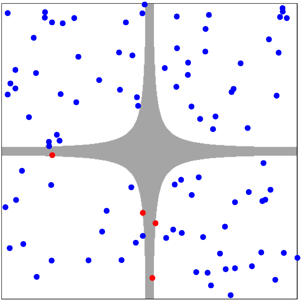
6 Line Darts

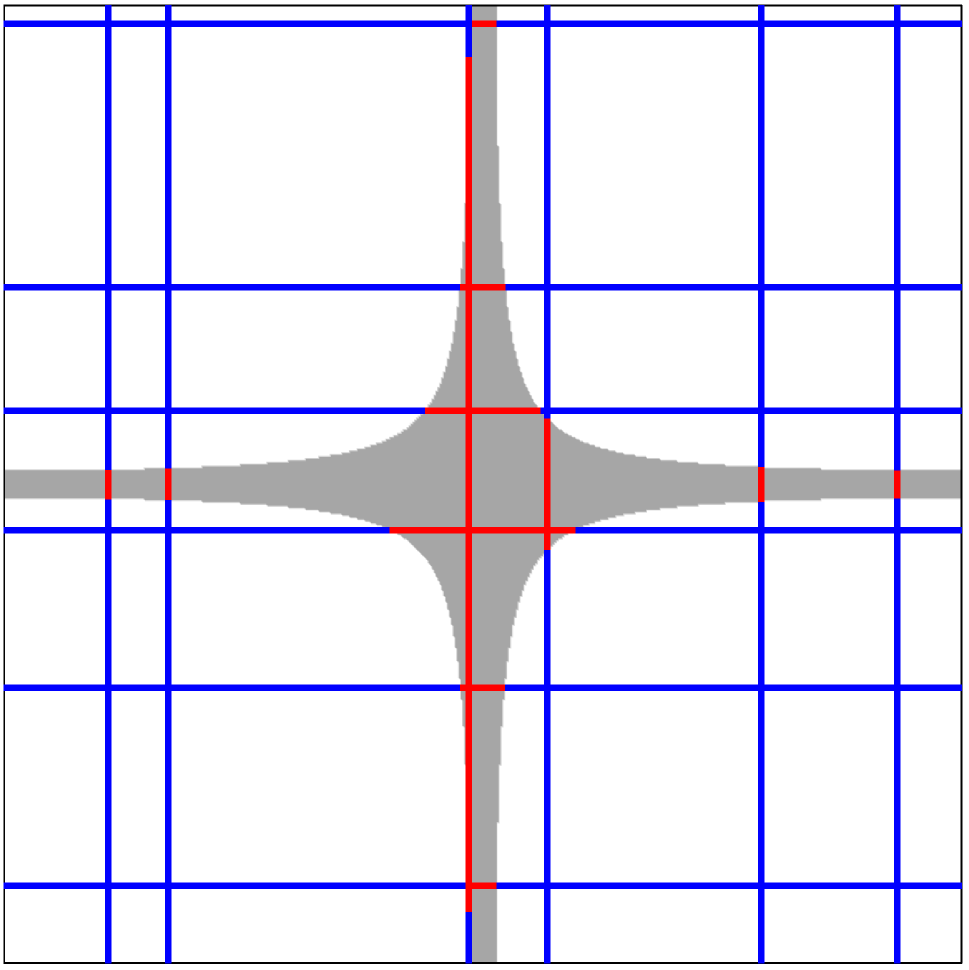
1 Plane Dart

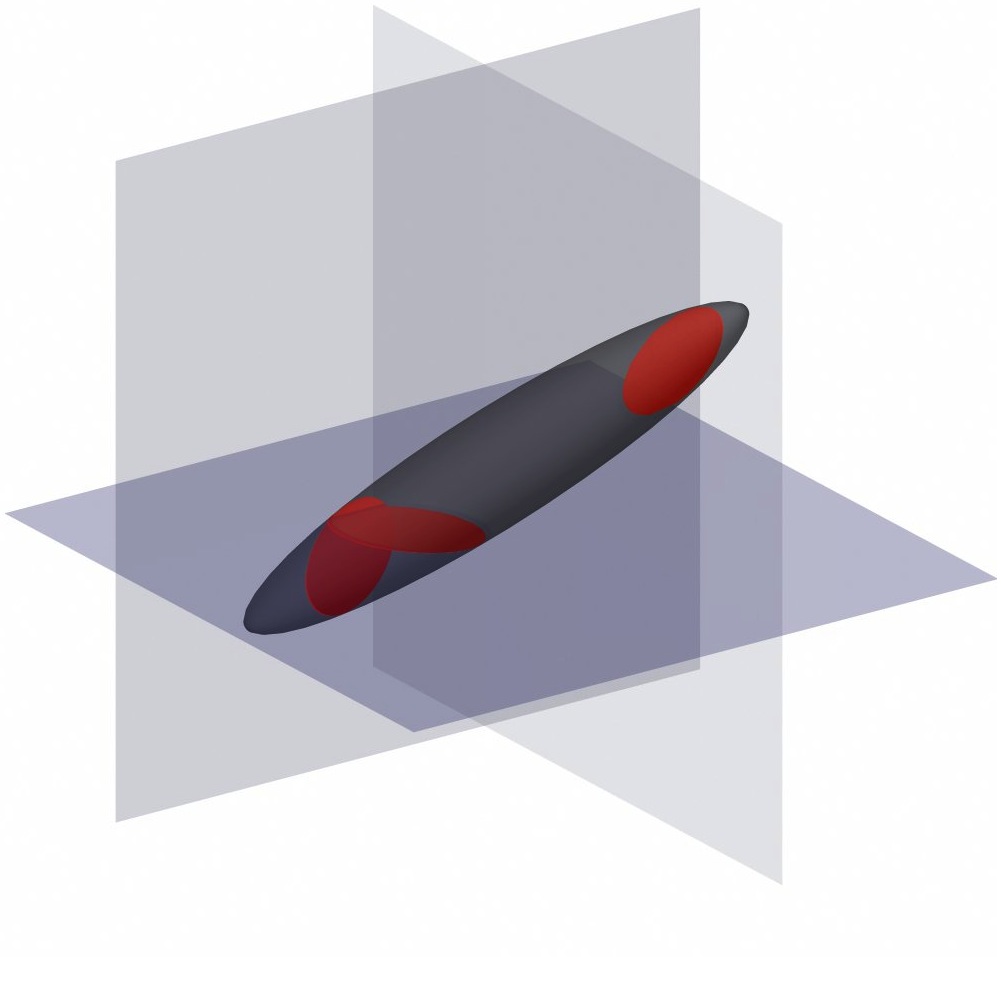
Figure 1: Sampling long and thin subregions (gray) using points (left), lines (center), and planes (right). Point samples may be cheap to generate and evaluate, but they contribute nothing to the final result if they miss the region of interest. Misses (blue) are frequent for regions with a small volume. Samples of higher dimensions, or $k$-d darts, often intersect (red) the region of interest, especially if the region is long and thin. A $k$-d dart’s greater expense is offset by it providing more information.

In many applications we are interested in estimating some global property of a function because it is difficult to calculate that property exactly. Sampling is the process of randomly selecting samples, subsets of a domain. The function is evaluated at these subsets, and the global property is estimated based on those values.

In typical sampling processes, the samples are points. However, a recurring challenge is to deal efficiently with the case that the interesting part of the domain is very small compared to the entire domain. For example, suppose we have a function over a domain, and we are interested in estimating the volume of the subdomain where the function is negative. If this subdomain has a very small volume, only a correspondingly very small fraction of uniform sample points will land in it; see Figure 1. Consequently, point sampling will require a large number of samples to get any estimate, and will be inefficient since most samples will not contribute.

We propose the $k$-d dart to address this problem. One key idea is that rather than evaluate the function at a single point, we evaluate it in a higher-dimensional region. For each sample, we evaluate the function along a set of higher-dimensional flats (i.e. lines, planes … hyperplanes). The second key idea is to use a set of mutually orthogonal flats, aligned with the coordinate axes; a $k$-d dart denotes this set of flats. Randomly oriented flats have been considered before, but orthogonal flats are more efficient and have better worst-case performance when probing high aspect-ratio settings. To ensure that the expected mean of the function estimates is correct, each of these flats is chosen independently. An important case of flats are one-dimensional lines. Using our previous example, we may find the points along the line where the function value is zero, then partition the line into segments where the function value $f$ is strictly positive or negative, and finally estimate the volume where $f<0$ from the negative-interval lengths. While these samples are more expensive to compute, they are more powerful; depending on the function they can generate better results for the same amount of effort.

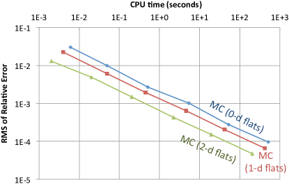
(a) Monte Carlo Sampling (MC)

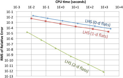
(b) Latin Hypercube Sampling (LHS)

Figure 2: Estimating the volume of a sphere using random sampling via $k$-d flats, k = 0, 1, 2. For each sample size, we performed 100 experiments and calculated the RMS error. The reported CPU time is the total time consumed by these experiments. For MC sampling (a) plane samples consumed an order of magnitude less time to achieve the same error as point samples. The savings were even more for LHS (b).

A simple example that demonstrates this concept is estimating the volume of a unit sphere by sampling from its bounding box: $f=-1$ inside the sphere and $0$ outside it, and we seek an estimate of $\int_{f<0}1$. Figure 2 shows the relation between error and time as the size of the sample increases. We sampled using $k$-d flats of dimension $k=0,1,2$. For a point sample, we checked if the point was inside the sphere. For higher dimensions, we calculated the fraction of the flat inside the sphere; see Figure 3. We performed both Monte Carlo (MC) and Latin Hypercube Sampling (LHS). For each sample size we ran 100 experiments and calculated the error in the volume estimate. Plane samples consumed less CPU time than point samples for the same RMS error. For MC sampling the payoff was about a factor of 5, and for LHS sampling the payoff was 3 to 8 orders of magnitude! The reasons behind these gains are the following:

• Evaluating $f$ along $k$-d flats is cheap; in this case we exploited the analytic function of the sphere.

• A $k$-d flat gives more information as $k$ increases.

• A flat is cheap to generate. Each $k$-d flat requires $d-k$ random numbers; here $d=3$.

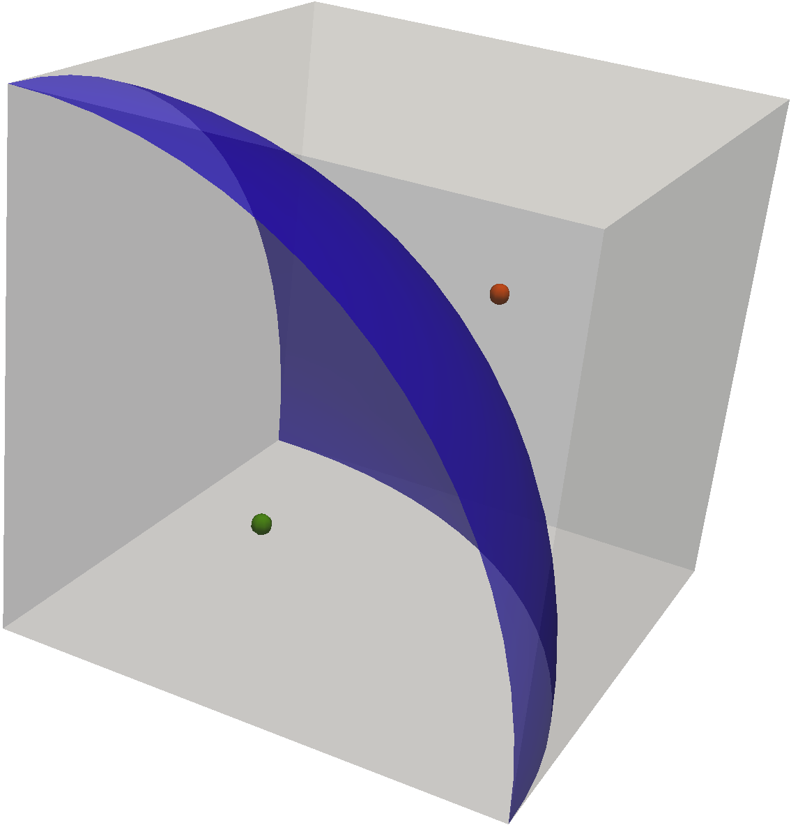
(a) 0-d flats

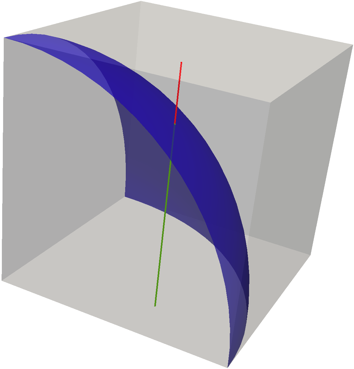
(b) 1-d flat

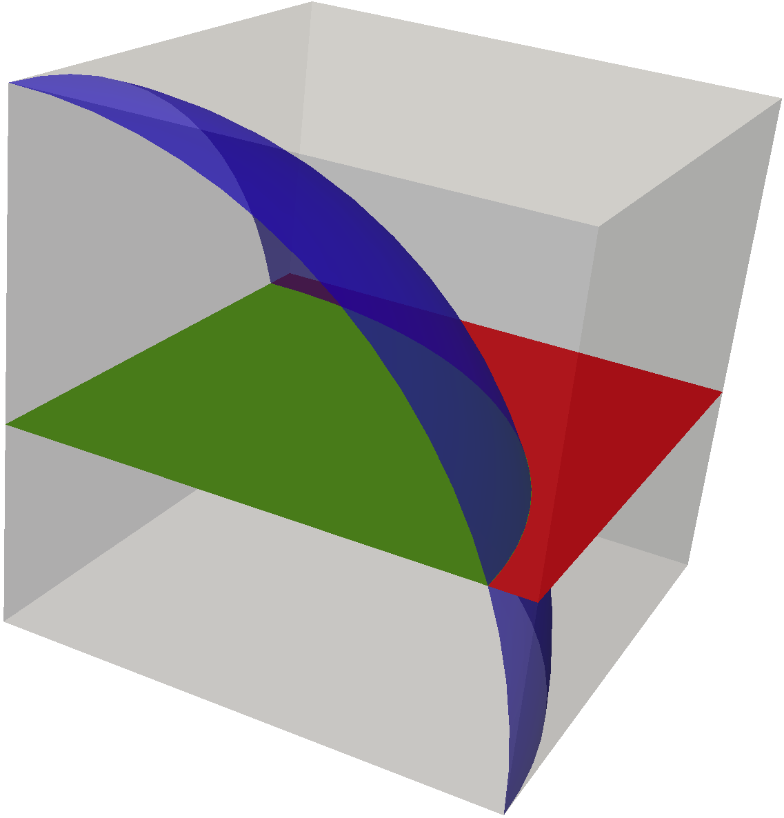
(c) 2-d flat

   

Figure 3: $k$-d flats used to estimate the volume of a sphere. The fraction of the sub-flats inside the sphere estimates the function average.

In general, evaluating the integration function along a $k$-d flat costs more than at a single point. However, for many problems, this extra cost is offset by the superior capability of a $k$-d flat to capture narrow regions. For instance, consider Figure 4(a), where a line flat perpendicular to that narrow region of interest will capture it regardless of its thickness. On the other hand, the probability of a point sample landing in the region approaches zero as the thickness decreases.

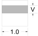
(a) Thin object

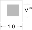
(b) Cubic object

Figure 4: Extreme subregion shapes. In general, a $k$-d flat has a better chance to intersect a region of interest as $k$ increases. For a given region volume, the advantage is higher for stretched regions than for square ones.

The purpose of this paper is to formalize and demonstrate the $k$-d dart approach. In Section 4, we show three practical applications: completing a relaxed maximal Poisson-disk sampling, in dimensions 4–30; rendering depth-of-field blur in four dimensions; and estimating the probability of failure from a response surface for uncertainty quantification, where the probability is small, e.g. 1e-5, and the dimension is large, e.g. 15. In each of these three applications the space is of moderate dimension, and line darts are particularly effective. The experiments in Section 5 verify the accuracy of higher-dimensional darts, using a volume estimation application.

2 Previous Work

Our work generalizes sampling. There are many patterns for generating samples. For graphics, maximal Poisson-disk sampling (Section 2.1) is common. Much prior work focuses on dimensions 2 and 3, but our interests extend beyond. Rendering applications use sampling in many forms (Section 2.3), often with high dimension. The field of uncertainty quantification (non-graphics, Section 2.4) attempts to quantify the range of a computation, typically by performing the computation many times with a well-distributed selection of input parameters. This is important in computational science for predictions and reliability.

Our $k$-d dart is a particular conception of high dimensional sampling. Line sampling has been explored in varied contexts already, within graphics and other domains. Unfortunately much of this work is isolated and does not consider dimension as a free parameter; we hope to help provide a unified view of these approaches.

Lines were used early in the history of Monte Carlo sampling. For instance, “Buffon’s needle problem” was published in 1777. It considers the number of intersections of randomly-oriented short line segments with axis-aligned regularly spaced infinite lines. Its solution involves geometric probability, either through integral geometry [25] or MC experiments [12], and gives an estimate of the value of $\pi$. Both the needle problem and volume estimation by line darts use finite objects, varying orientations, and infinite probes; but which things are known, measured, and estimated are different, as are which quantities are uniform-random and which are uniform-deterministic. For example, using sets of orthogonal flats means the indices of the fixed dimensions of our flats are evenly spaced deterministically, whereas in Buffon’s problem the geometry of the rule lines are evenly spaced.

In neutron transport physics simulations, a class of Monte Carlo algorithms known as “track length estimators” essentially performs Monte Carlo estimation using line segments [28]. This is in contrast to the “collision estimators” class that estimates using point samples. In graphics, these collision estimators correspond to standard volumetric photon mapping, estimation using photon scattering locations. Also track-length estimators (using line samples) correspond to photon beams; estimation uses entire random-walk path segments [14]. In surface reconstruction and CAD modeling, we can count the intersections of unoriented line samples with the surface, then make use of the integral geometry Cauchy-Crofton formula to estimate integration quantities such as surface area or enclosed volume [19]. To get the right estimate with low variance, it is crucial to select the sample lines using the right probability model. For example, models for bundles of uniformly-spaced parallel lines, reminiscent of both $k$-d darts and the regularly spaced lines in Buffon’s needle problem; models for chordal lines; and pseudo-random and other numerical sequences have all been studied in the context of sampling surfaces [26].

2.1 Relaxed Maximal Poisson-Disk Sampling

Maximal Poisson-disk Sampling (MPS) is a popular graphics technique to distribute a set of points in a domain. The points are random and have a blue-noise spectrum, which is well-suited to the human visual system and helps avoid visual artifacts. The points have a minimum distance between them, $r_{f}$, which helps to use the point budget efficiently. We denote the maximum distance from a domain point to its nearest sample by $r_{c}$. In a maximal sample, the $r_{f}$ disks around the points overlap to cover the whole domain, leaving no room to add another point, and $r_{c}\leq r_{f}$. Otherwise, maximality is relaxed, and we measure how far the geometry is from maximality by the distribution aspect ratio $\epsilon_{r}=r_{c}/r_{f}\geq 1$. Point clouds with a meaningful upper bound on $\epsilon_{r}$ are separated-yet-dense, also known as “well-spaced.”

MPS algorithms abound, and often achieving maximality is the most challenging part. In some applications maximality is not required [17]. The acceptable relaxation of maximality depends on the application. For example, in Voronoi mesh generation [4], the cells have an aspect ratio bound that varies smoothly with the relaxation, $2\epsilon_{r}$. Some methods sacrifice maximality to terminate more quickly, but explicit statements about the achieved $\epsilon_{r}$ are rare.

Many methods use some form of a background grid for point location and proximity queries [6, 15, 32]. The background grid may be refined, as in a quadtree, to track the remaining voids (uncovered regions) [7, 33]. This can be made efficient in dimensions up to about 5 [5]. However, even in dimensions below 5, refinement methods can run out of memory as the sample size increases. Memory problems are exacerbated on a GPU.

Uncertainty quantification motivates MPS sampling in higher dimensions, e.g. 10–30. No MPS methods in the literature scale to these dimensions due to the so-called “curse of dimensionality.” Classical dart throwing [2, 3] is not strongly dependent on dimension, but as the number of accepted samples increases, the runtime for the next sample becomes prohibitive and the algorithm must terminate well before maximality.

Consider sampling a unit box with disk radius $r$ in dimension $d$. Some issues are fundamental to the problem, independent of any specific algorithm or application. The size of a maximal sampling $n$ is indeterminate, but its lower and upper bounds grow exponentially in $1/r$ and $d$. The kissing number, the number of disks that can touch another disk, grows exponentially in $d$. (The geometry literature discusses these issues extensively. The densest packings and largest kissing numbers by dimension are summarized in “A Catalogue of Lattices” [23].)

The curses of dimensionality for grid-based methods go beyond those unavoidable issues:

1. The base grid size grows exponentially and faster than the output point set.

2. A grid cell is refined into $2^{d}$ subcells.

3. The number of nearby cells that might contain a conflicting sample grows faster than the kissing number.

4. The ratio of misses/hits grows exponentially with the dimension [5].

Item 1 arises because the size of the base grid is usually chosen such that each cell can accommodate at most one point: base squares have diagonal length $r$ and edge length $r/\sqrt{d}$. Worse, at maximality, the number of empty base cells grows exponentially with the dimension. These empty cells increase the time, and especially the memory requirements, to prohibitive levels. One possible solution is to choose a base grid level with edge length $2d$, so that every square must contain one point. However, due to Item 2, this approach just defers the problem until cells are required to be refined a couple of times to represent voids. Because of the kissing number, representing voids through geometric constructions [6] or explicit arrival times [15] do not appear to be viable solutions at high dimension.

Some approximate methods [32] put an upper bound on the number of misses per cell, which partly addresses Item 4. The drawback is that the sampling is not maximal. How far it is from maximality has not been analyzed, but volume arguments suggest that for a fixed box size, the number of allowed misses must grow exponentially in $d$ to bound the linear distance between an uncovered point and a sample’s disk.

While some of these issues affect runtime, the real curse is the memory requirements for quadtrees. Simple MPS [5] is the quadtree method with the best memory scaling by dimension. It seems unlikely to extend to even $d=10$ in the near future. Simple MPS uses a flat quadtree of same-sized squares, periodically refining all remaining squares uniformly. We compare our results to Simple MPS in Section 4.1.4.

2.2 Motivation for High-Dimensional Point Clouds

In the design of computer experiments, we generate points in parameter space, then evaluate a function at the sample points. We often build a surrogate model based on those points’ values, e.g. Kriging models. The dimension is equal to the number of parameters, so can be very high. The time it takes to generate the points is often very small compared to evaluating the function, so it is worthwhile to spend the time to find a set of points that span the space efficiently. Well-spaced points use the point budget efficiently, and provide bounds on the condition number and interpolation error.

For some applications, if the function is not too expensive, it may make sense to sample the function directly using $k$-d darts. For example, if the integral of a function over a flat is available analytically, then sampling it directly using $k$-d darts would be very efficient. Otherwise, $k$-d darts can provide well-spaced points (see Section 4.1); we can build a surrogate model over those points; then $k$-d darts can integrate the surrogate model analytically.

Another application where sample points are required is finite element simulation, where we need a computational mesh of the points.

2.3 Rendering

High-quality rendering is an important application of multi-dimensional sampling. Photorealistic effects like motion blur, depth-of-field (defocus) and soft shadows can be expressed as integrals over multiple dimensions. Classical techniques often employ stochastic point sampling to estimate these integrals. Noise-free rendering using point sampling can require a large number of samples, which can be extremely expensive for complicated scenes.

Thus a long history of research has targeted choosing samples wisely. Mitchell’s classic antialiasing paper [22], for instance, “focus[es] on reducing sampling density while still producing an image of high quality,” primarily in the context of ray tracing. Metropolis light transport [31] “performs especially well on problems that are usually considered difficult” by using mutations to preferentially (but in an unbiased way) sample light paths in interesting regions of the path space.

Besides choosing samples carefully, another approach toward the same goal is to reduce the number of required samples through techniques such as sample reuse and/or caching. For example, a notable recent advance in this area, by Lehtinen et al. [18], specifically notes “a clear need for methods that maximize the image quality obtainable from a given set of samples” and exploits anisotropy in the temporal light field to reuse samples between pixels. Our work has a similar goal—making the best use of a limited number of samples—but instead reduces the number of necessary samples by increasing their dimensionality.

$k$-d darts formalize a general way of multi-dimensional sampling. Several early graphics applications use multi-dimensional samples in limited and specific scenarios. The OpenGL accumulation buffer [11] uses a form of $k$-d darts for motion blur: each output pixel is an aggregate of several input pixels, each of which may span a 2-d region (pixel area) for a constant shutter time. Essentially, the accumulation buffer samples 2-d $x$-$y$ images in a 3-d $x$-$y$-time space. Nelson Max [20] uses a scan-line visible surface algorithm that generates line samples, describing how to use the information in these samples to create antialiased images.

Recent research has also shown promise in rendering high-quality motion blur using multi-dimensional samples. Gribel et al. [10, 9] present the use of line samples (our “1-d flats”). In their 3-d domain ($x,y,t$) they fix $x,y$ and perform a 1-d flat in the $t$ domain. They also extend their implementation to render motion-correct ambient occlusion.

More recently, line samples have proven useful in the representation of light. Sun et al. [29] represent lighting and viewing rays directly in a 6-d Plücker space, which allows an efficient formulation of finding nearby lighting rays. This, in turn, allows accurate, fast rendering of large scenes with single scattering even in the presence of occlusions and specular bounces. The previously mentioned work of Jarosz et al. [14] concentrates on better representations for light paths in photon tracing for the purposes of rendering participating media in light interaction; previous methods had used photon particles. Instead, they represent and store full light paths (samples), resulting in a more compact and expressive lighting representation with corresponding performance benefits.

Jones and Perry [16] experimented with using analytical line sampling for anti-aliased polygon rendering. They shoot single-dimensional darts across a pixel’s surface, analytically compute triangle coverage for each of them, and then average them to obtain pixel colors.

Our paper generalizes the idea of multi-dimensional darts for sampling, and it is this generalization that helps us design renderers that use $k$-d darts in different configurations. For rendering depth-of-field effects with added anti-aliasing, we present a generalized configuration using a full 1-d dart in Section 4.2. That is, we use a set of orthogonal flats rather than just a single flat as in prior work. We compute high-quality depth-of-field images efficiently.

While we demonstrate just one configuration of $k$-d darts, several different strategies are possible for depth-of-field and other effects. In general, $k$-d darts offer a sampling process that converges faster and has lower noise than point sampling; the use of $k$-d darts offers the potential benefit of faster convergence but must be weighed against the higher complexity per $k$-d dart.

2.4 Monte Carlo Sampling

Random sampling is one of the oldest [12] and most robust methods for uncertainty quantification. The principal use of Monte Carlo (MC) sampling is to approximate a high-dimensional integral with a sample mean. The primary drawback of MC is the slow rate at which the sample mean converges to its true value. The standard error in the computed mean for $n$ samples is

$$\sigma_{\mathrm{err}}=\frac{\sigma}{\sqrt{n}}.$$ (1)

Although this rate of convergence in $n$ is very slow, the number of dimensions, $d$, does not appear in Equation (1). MC’s primary advantage is that it is not subject to the curse of dimensionality. Significant effort has been invested in developing variants of MC with faster rates of convergence; a full review is out of scope. Latin Hypercube Sampling (LHS) [21, 24] is known as “N-rooks sampling” in the graphics community. Importance sampling [8] involves preferentially sampling rare cases and compensating by reducing their weight.

3 Dart Framework

Given the ideas of the method (Section 1) and where it might be useful (Section 2), we now define it formally and give a general recipe for converting a point sampling algorithm to a $k$-d dart sampling algorithm. We consider two application scenarios. The first is sampling to evaluate a function, as in numerical integration; see Section 3.1. The second is sampling to find locations in the domain where the function has a particular value; see Section 3.2.

We begin with terminology. Function $f$ is defined over domain $\mathcal{X}\subset\mathbb{R}^{d}$. Often $\mathcal{X}=[0,1]^{d}$. A flat $F$ is a $k$-dimensional subspace of the domain, the vector space defined by fixing $d-k$ coordinates. A $k$-d dart $s^{k}$ is a sample defined by a set of $I=\binom{d}{k}$ $k$-dimensional flats, $s^{k}_{i}$, one for each combination of fixed coordinates. So in $\mathbb{R}^{2}$, a 1-d dart might consist of the two 1-d flats at $x=0.5$ and $y=0.5$.

3.1 Evaluating a Function over a Domain

Consider an algorithm that receives a single value, $y=f(x)$, from evaluating a function $f$ at a uniform random point $x$. To get an analogous single value $y^{\prime}$ from a $k$-d dart, we calculate the average of $f$ over its flats, weighted by the relative measure of the flats. We generate a $k$-d dart’s flats one at a time. For each flat $F$ we choose its fixed coordinates uniformly at random, then:

1. Clip $F$ at the boundary of the domain and estimate its relative volume $|F|=\int_{F}1$. For the unit box this is trivial.

2. Integrate the function along the clipped flat: $G=\int_{F}f$.

3. Now the weighted average of $f$ over the flat is simply the ratio of these two computations: $H=G/|F|$.

Then $y^{\prime}$ is simply the average of $H$ over the flats: $y^{\prime}=\sum_{i=1}^{I}H_{i}/I$. We can combine multiple $k$-d dart $y^{\prime}$ measurements in the same way that we might combine measurements made at multiple point samples. Thus we can convert point-sampling function evaluation to $k$-d dart function evaluation.

A generic approach (for any $k$-dimensional flat) is to use numerical integration over a discretization of the flat. Represent a flat with a uniform grid (mesh). (We assume it is too expensive to mesh the entire domain.) In (1), clip the grid elements at the domain boundary, generating simplices. In (2), evaluate $f$ at the grid points and perform standard numerical integration over the grid simplices.

Our depth of field, probability of failure, and volume estimation applications follow this recipe, because they use Monte Carlo integration, but the integration along the line flats can be made faster and more accurate given application-specific knowledge about the function. For probability of failure, the function we integrate is the 0–1 indicator function of failure, rather than the continuous value of the response function. We improve accuracy by finding the roots of a single-variable equation to find the boundary points where the indicator function switches its value. For depth of field, $f$ is the contribution of one ray (photon) to a pixel, and we seek to estimate the contribution of all photons over all focal depths for each pixel. For efficiency we use discrete algorithms to find the occlusion boundaries of triangles, then integrate a continuous function over each non-occluded segment of a triangle.

3.2 Identifying Points in the Domain with a Particular Function Value

MPS represents a different category of application. In this application, instead of integrating $f(x)$, we are looking for a random $x$ that satisfies $f(x)>0$, i.e. finding a point outside all prior disks. Point-sampling techniques would sample the domain until such a point was found, which is expensive if the region of interest is small compared to the size of the domain. Instead, we can use $k$-d darts for sampling using the following generic recipe:

1. Clip $F$ at the boundary of the domain. Retain $g$, a representation of the clipped flat. (For MPS, we clip a line by the unit cube.)

2. Retain the portions of $g$ where the function has the particular value of interest, e.g. $f>0$. (For MPS, these are the subsegments outside all prior disks.)

3. Return a random point from $g$.

4 Applying the Framework

We now describe how to apply the $k$-d dart framework to our representative applications in more detail.

4.1 Relaxed MPS

  while maximality estimates are inadequate do

     generate a line dart $s^{1}$

     for all $i=$permutation$(1..d)$ do

        generate line segments $g=s^{1}_{i}\cap$ domain

        for all samples $p$ do

           subdivide $g=g\setminus D(p)$

        end for

        if $g\neq\emptyset$ then

           count $s^{1}$ as a hit

           select a sample point uniformly from $g$

           skip to next line dart

        end if

     end for

     count $s^{1}$ as a miss

  end while

Algorithm 1 A classical dart throwing algorithm using line darts.

Our relaxed maximal Poisson-disk sampling algorithm is a variant of traditional dart-throwing, throwing point darts and keeping those that hit an uncovered region (void). Algorithm 1 specifies our implementation in detail; in brief, we cast a line dart into the domain and intersect it with the disks of previously accepted samples to generate a set of uncovered segments, then uniformly sample from those segments with a point dart. The user specifies an acceptable void volume $V$, the fraction of the domain uncovered by sample disks. We have a conservative stopping criteria based on the number of successive misses that usually achieves a smaller void volume. Figure 5 can be used as a guide for selecting $V$ in four dimensions.

4.1.1 Complexity

The memory requirements are only $O(nd)$, which is what is required to represent the output point cloud because each sample has $d$ coordinates. Only $2n+d$ floats are needed for scratch space for line segments $g$. We may generate and store only one flat of one dart at a time. The runtime is $O(dn\log n+nd^{2})$ per dart throw. The most significant feature is that the complexity does not suffer from a curse of dimensionality: there are no exponents containing $d$. The number of throws is a function of $V$ and the miss rate; the community appears to lack the tools to analytically bound the miss rate, but we show that for line darts it can be made to be reasonable, or at least more reasonable than the alternatives.

Our approach is efficient because a line dart is more likely to intersect an uncovered region than a point dart. Only extremely simple and one-dimensional data structures are needed. The cost of throwing a line dart is nearly the same as a point dart.

4.1.2 Output and Process

The main drawback is that the output is not maximal, but its deviation can be estimated. A second potential drawback is that the process is not identical to MPS. There is no proof that the expected outputs are the same. Indeed, for a non-maximal sample, the probability of inserting the next sample point in a given disk-free subregion depends only on the subregion’s area in MPS; but for our variant the probability depends also on how much prior disks cover the axis-aligned lines through the subregion. The main effect appears to be the order in which points are introduced, rather than their spatial distribution near maximality. Choosing the position of the next sample is dependent on many prior random decisions, so there are few noticeable patterns between one run and another with a different random number seed.

MPS and Algorithm 1 follow a different process. The quality of the outcome, the point positions, does not appear to be sensitive to this, and we see little distinction between the outputs using the standard measures of FFT spectrum, power, and anisotropy. Additionally, we are unaware of any formal definition of an ideal point cloud nor any proof that MPS produces it, so exactly matching the MPS process and its output are not strict requirements. The conventional goal in the graphics literature is “blue noise,” meaning no discernible axis or boundary aligned patterns, and something resembling a Heaviside step function for the mean radial power, as in Figure 10 right.

4.1.3 Implementation Details

$k$-d Tree

To speed up the iteration over prior samples when generating segments $g$ we use a $k$-d tree. This allows us to prune samples whose disks are too far away to intersect the line of $s^{1}_{i}$. A $k$-d tree requires little memory regardless of the number of dimensions.

Line Segments $g$

Beyond the $k$-d tree and storing the accepted samples, our only data structure is $g$, an array of segments in the line of $s^{1}_{i}$. Each stored segment is inside the domain but outside the sample disks processed so far. The set $g$ may be implemented as a one-dimensional linked list storing the $i$th coordinate of the starts and ends of segments: $g=[a_{0}b_{0}a_{1}b_{1}\ldots a_{q}b_{q}]$ where $q\leq n$ if the domain is convex.

To update $g$ for a new disk $D(c)$ centered at sample $c$, we first compute $g^{\prime}=D(c)\cap l=[b^{\prime},a^{\prime}]$. Using binary search in $O(\log n)$ time, we find the position in $g$ where $b^{\prime}$ and $a^{\prime}$ should appear. If they are beyond $a_{0}$ or $b_{q}$, the disk does not intersect $g$. If $b^{\prime}$ and $a^{\prime}$ both lie between $a_{j}$ and $b_{j}$, the latter segment is split into two: $a_{j}b^{\prime}a^{\prime}b_{j}$. Otherwise, if only $b^{\prime}$ lies between $a_{j}$ and $b_{j}$, then a segment is trimmed by replacing $b_{j}$ by $b^{\prime}$; a similar step applies for $a^{\prime}$. Any endpoints between $b^{\prime}$ and $a^{\prime}$ are covered by the disk and discarded. The updates are $O(1)$ time for a linked list.

To choose a point from $g$ uniformly, we sum the lengths of the segments $L$, choose a random number between $0$ and $L$, and use binary search to find the corresponding point on $g$.

Maximality Estimates

The user sets the remaining void volume $V$ that is acceptable. Here we show how to translate that into a conservative stopping criteria. Denote the probability of hitting the void with a $k$-d dart by $P_{k}$. Given a lower bound on $P_{k}$, we set $m\geq\lceil 1/P_{k}\rceil.$ We stop after $m$ consecutive misses.

We seek lower bounds on $P_{k}$ in terms of $V$ in order to find a sufficiently large value of $m$. For point darts, $k=0$ and $P_{0}=V$ regardless of void shape. For higher dimensional darts, the worst shape for a void is a hypercube with edge length $b=V^{\frac{1}{d}}$. By worst shape, we mean the shape that has the smallest $P_{k}$ for a fixed $V$, assuming the entire domain is a hypercube. For a hypercube void, the probability of hitting that void with a $k$-d flat is given by $p_{k}=V^{\frac{d-k}{d}}$. A $k$-d dart contains $l_{k}={d\choose k}$ $k$-d flats and hence $P_{k}=1-\left(1-p_{k}\right)^{l_{k}}$. This gives a lower bound on $P_{k}$, and a sufficient value of $m$. We may consider this as a MC estimation of the remaining void using a sample size of the last $m+1$ $k$-d darts. As in any MC process, there is some variance, which decreases as $k$ increases. Moreover, the remaining void is typically scattered throughout the domain; $r_{c}$ is less than if the void volume was a single ball.

4.1.4 Experimental Results

Distribution Aspect Ratio

The free radius, $r_{f}$, is the disk radius, the minimum distance between any two samples. The coverage radius, $r_{c}$, is the maximum distance between a domain point and its nearest sample. We define the distribution aspect ratio as $\epsilon_{r}={r_{c}}/{r_{f}}\geq 1.$ This is a measure of maximality.

To compute this for a point cloud, we used Qhull [1] to generate a Voronoi diagram. For each Voronoi vertex we retrieved the distance to its closest sample point: $r_{c}$ is the maximum of these distances.

Figure 5 shows the relation between the average distribution aspect ratio and the acceptable void volume over four-dimensional samples of two different disk-free radii: $r_{f}=0.1$ and $r_{f}=0.05$. Figure 7 shows run-times for generating the point clouds. Line darts consistently produced better results.

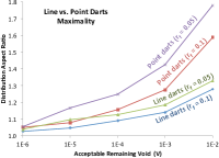
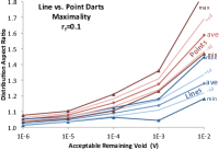
Figure 5: Achieved distribution aspect ratio for void volume threshold $V$ in $d=4$. Data points are averages over 25 experiments. Right shows more statistics for $r_{f}=0.01$, including standard deviation, sd.

Speed of Approaching Maximality

We tested our code over 2, 4, 10, and 30-dimensional domains using point darts and line darts. Figure 8 shows the number of points inserted over time. The expected void volume $V$ is related to the number of points; in practice the number of inserted points is a better indicator of maximality than our loose estimates of $V$ based on successive misses. Line darts were able to generate larger samples for all $V$ and $d$.

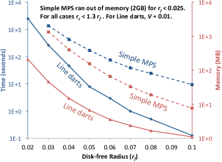
Figure 6: Time (blues) and memory (reds) for line darts compared to Simple MPS for the same acceptable void volume, $V$=1e-2.

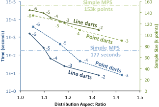
Figure 7: $V$ threshold effects on time (blues) and sample size (greens) for line and point darts. Data points are labeled with $\log_{10}V$. As $V$ decreases, the sample approaches maximality and distribution aspect ratio 1. Simple MPS [5] dashed lines are for a maximal distribution.

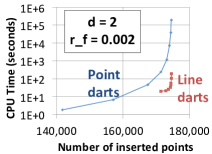
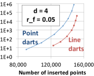
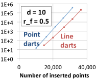
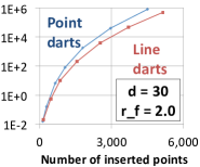
Figure 8: Line darts approach maximality faster than point darts, as measured by the number of inserted points in a given run time.

Efficiency by Method

Figure 6 compares the performance of traditional point darts and line darts (this work) to Simple MPS [5]. Recall Simple MPS is based on a flat quadtree, and is currently the fastest and most memory-efficient of the provably-correct MPS methods. Our method is attractive at large values of $r_{f}$ for its speed, and at low values of $r_{f}$ for its memory consumption. For example, for $r_{f}<0.025$, we generated 4M points in half an hour using 107 MB of memory, while Simple MPS ran out of memory at 2 GB.

Output Quality

We measure the quality of the distribution of 2-d output points using the PSA spectrum analysis tool [27]. Using point darts, our process is the same as classic dart-throwing, so we it for our standard of correct output. Figures 9 and 10 compare the outputs’ blue-noise properties; the difference between point and line darts was insignificant, at least for these three metrics.

   

(a) Line darts

   

(b) Point darts

Figure 9: FFT spectra (right) for the relaxed MPS point clouds (left) generated by line darts (top) and point darts (bottom).

   

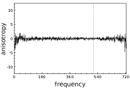
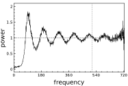
(a) Line darts

   

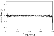
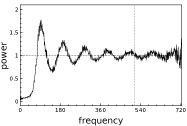
(b) Point darts

Figure 10: Radial anisotropy and mean power estimates for line darts (top) and point darts (bottom), averaged over ten samplings.

4.2 Depth of Field With Antialiasing

$k$-d darts can be used for fast and high-quality rendering of depth-of-field (DOF) effects in computer-synthesized images. Mathematically, computing a pixel’s color in the presence of DOF can be expressed as a four-dimensional integral over the pixel’s spatial $(x,y)$ and lens aperture $(u,v)$ dimensions. In most high-quality renderers, this is calculated using Monte Carlo integration over many point samples. This method suffers from a low rate of convergence; reducing noise for a good quality image usually requires a very large number of samples per pixel. $k$-d darts offer the promise of faster convergence with low noise. Instead of using point samples for reconstruction, we use 1-d (line) darts, thrown in the 4-d $(x,y,u,v)$ space.

We use Latin Hypercube Sampling (LHS) or jittered sampling for each dimension [2]. Given that our sample space is four-dimensional, each line dart consists of four line flats. We select $n$ points, i.e. $4n$ flats. Each line requires a fixed location in 3-d and a variable fourth dimension.

We compute coverage for these darts using a method inspired by Gribel et al.’s work [10, 9] on rendering motion blur. Gribel et al. fix $x$ and $y$ and shoot line samples in the time domain; instead, we use line darts that shoot line flats in all spatial dimensions to compute depth-of-field blur. We also sample a higher-dimensional problem.

4.2.1 Contrast to Tzeng et al.

Tzeng et al. [30] considered line sampling for DOF. They only consider the two $(u,v)$ dimensions, not the four $(u,v,x,y)$ dimensions as we do. Further, they take advantage of the structure that the $(u,v)$ subspace of interest is uniformly circular. This reduces 2-d $(u,v)$ sampling to 1-d sampling of lines through the origin, pinwheel sampling by angle. In their implementation, for each pixel, they fix $x$ and $y$ and use a pinwheel of line samples to vary $u$ and $v$. The resulting DOF had high performance when compared to point sampling strategies, with low noise. However, due to both the pinwheel configuration and the fixing of $x$ and $y$ for each pixel’s sample, strobing artifacts tended to occur in regions with high frequency changes. The formulation we present in this paper differs in the following ways:

• Both implementations address DOF, but we also address antialiasing.

• Tzeng et al.’s line darts are all radial and specified completely by their angle; they live in 1-d $(\theta)$ space. In this paper, we use axis-aligned darts in 4-d $(x,y,u,v)$ space. The positive and negative consequences follow:

  • Tzeng et al. exhibits screen-space aliasing because $x$ and $y$ are fixed.

  • Tzeng et al. achieves higher quality DOF for the same number of samples, because 1-d spaces require fewer samples to cover than 4-d spaces.

• Tzeng et al. use non-random dart locations, but we randomly position darts.

• Tzeng et al.’s work specifically targets the GPU pipeline; we do not discuss (or consider) implementation details.

4.2.2 Triangle Edge Equations in 4-d

We now describe the triangle equations and how we create a line sample. For a given triangle, we start by computing a signed radius of Circle of Confusion (CoC) for each vertex, obtained using the following expression [13]:

$$\textnormal{CoC}=A\frac{f(z-z_{f})}{z(z_{f}-f)},$$

where $A$ and $f$ are the camera aperture and focal length, respectively, and $z_{f}$ and $z$ indicate the respective depths of the focal plane and the given vertex. Note $z$ is simply the $w$ coordinate of the vertex in clip space. Now that we have the circle of confusion for each triangle’s vertex, we can begin formulating a sampling strategy for each pixel.

Given a set of coordinates on the lens $u$ and $v$, we assume a linear apparent motion of the vertex screen coordinates. For a given screen space vertex $i\in\{0,1,2\}$, with coordinates $(x_{i},y_{i})$, circle of confusion $c_{i}$, and $u,v\in[-0.5,0.5]$, we have

$$x_{i}^{u}=x_{i}+c_{i}u$$ (2)

$$y_{i}^{v}=y_{i}+c_{i}v$$ (3)

For each pixel we have a four-dimensional space $(x,y,u,v)$, where $x$ and $y$ are the subpixel regions, and $u$ and $v$ are coordinates on the lens. To get a realistic and noise-free image, we seek to sample this space uniformly in an effective manner. Since we have four varying dimensions, we choose to use four different hypercubes for our Latin Hypercube Sampling (LHS). Each hypercube chooses three dimensions within which to sample, and one that will vary in our next stage.

For each triangle, we can consider the edge equations in this four-dimensional space to be the following: we substitute Equations (2) and (3) into the equations for testing whether a point $(x,y)$ lies within one of the triangle edges $i$. Let $ES_{i}$ represent the edge-sum at point $(x,y)$ for the $i$th edge, between vertices $i$ and $j$,

$$ES_{i}(x,y,u,v)=(y-y^{v}_{i})(x^{u}_{j}-x^{u}_{i})-(x-x^{u}_{i})(y^{v}_{j}-y^{v}_{i}).$$

Expanding, we get equivalent right-hand sides

$$\Leftrightarrow (y-y_{i}-c_{i}v)\left(x_{j}-x_{i}+u(c_{j}-c_{i})\right)$$

$$- (x-x_{i}-c_{i}u)\left(y_{j}-y_{i}+v(c_{j}-c_{i})\right)$$

$$\Leftrightarrow ES_{i}(x,y,0,0)$$

$$+ u\left(c_{j}(y-y_{i})-c_{i}(y-y_{j})\right)$$

$$- v\left(c_{j}(x-x_{i})-c_{i}(x-x_{j})\right).$$

This simplifies to

$$ES_{i}(x,y,u,v)=C_{i}(x,y)+uA_{i}(y)-vB_{i}(x)\geq 0.$$

Here we have four dimensions of variability ($x,y,u,v$). In conventional point sampling, one would randomly (or pseudo-randomly) select a set of points in this space. We instead decide to employ line sampling using our Latin hypercubes. To illustrate this concept, consider fixing three of these dimensions with points on our hypercube from LHS: select $x_{1},y_{1}$ and $u_{1}$ for $x,y$ and $u$. Now we have a line equation as follows:

$$ES_{i}(v)=C_{i}(x_{1},y_{1})+u_{1}A_{i}(y_{1})-vB_{i}(x_{1}),$$

which simplifies to

$$ES_{i}(v)=P-vQ.$$

This line equation is easy to analytically solve for each of our edge equations and determines where line coverage exists. The same concept can be extended to our other hypercube setups, fixing three of the dimensions and varying the last.

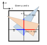
(a) Two line darts in $(x,u)$

(b) Resolving occlusion depth

Figure 11: Our technique for computing analytical coverage using line darts. In this example, consider two possible line flats in the $x$ and $u$ directions. The domain can be transformed and we can test the triangles for occlusion along the line flat as shown in (a). Depth resolution per flat is shown in (b).

4.2.3 Analytical Coverage in the Hypercube Domain

Knowing the edge equations in our 4-d domain, we can now compute their coverage along a line sample. Figure 11 summarizes our technique for determining coverage.

We instantiate a set of line flats along each of our four hypercube configurations. A line dart is the combination of four different line flats (one in the direction of each of the four dimensions of the domain) with initial points chosen using our LHS.

Rendering consists of testing each incoming triangle against potentially covered line flats. For each pixel sample in the triangle’s bounding box, we use equations from Section 4.2.2 to transform triangle edges to test for the correct hypercube domain.

To finish the calculation we follow Gribel et al.’s approach [10] to construct and resolve line darts.

For each line flat, we analytically compute its segment covered by the triangle. A per-line-sample queue stores the color and depth of covered segments. Once all triangles have been processed, we resolve the final color for each sample. We sweep across the flat while aggregating triangles closest in depth, and then use all pixel samples to compute the final color for the pixel.

4.2.4 Implementation and Results

To test our formulation, we built a simple CPU-based renderer. It is capable of rendering scenes using traditional triangle rasterization. We integrated two additional capabilities:

• A stochastic sampler based on point darts.

• A sampler based on line darts.

Table 1: Performance of our point vs. line darts.

Cessna	256 points	1024 points	16 lines	30 lines
time (s)	125	494	97	176
Teapot	256 points	1024 points	16 lines	30 lines
time (s)	214	853	157	292

The two noise artifacts that typically occur using a DOF scheme are noise in blurry regions and noisy aliasing artifacts near the point in focus. For scenes far away from the focal plane, line flats in the $x$ and $y$ direction become particularly narrow when compared to the sampling space, and this causes additional noise. In these regions the length of flats in the $x$ and $y$ dimensions are significantly smaller than flats in either the $u$ or $v$ direction.

If we consider all such flats to have equal contributions, this results in the $x$ and $y$ samples adding a noticeable amount of noise into our system in blurry regions. To address this, rather than considering all line flats to have equal contribution, we select a weight constant ($\alpha=0.2$ in our case) such that $x$ and $y$ line flats are scaled by $\alpha$ and contribute less to the scene.

This weight can be modified based on the aperture of the lens for the scene. In cases where the aperture is small, contributions from $x$ and $y$ are deemed more important (for antialiasing), and the weight is adjusted accordingly. A more accurate dart sampling method might also consider the ratios of flat lengths per tile (worst case) and decide on an $\alpha$ weight accordingly. Research is needed to determine the optimal amount for each flat to contribute. Still, our simple heuristic seems to be effective.

Figure 12 compares two scenes rendered with our point dart and line dart techniques. Renderings based on $k$-d darts are virtually free of noise and aliasing artifacts. Point darts, however, retain noticeable aliasing artifacts even with 1024 darts. Although 16 line darts produce a bit more noise in unfocused regions than 256 point darts, 30 line darts has better quality than 256 point darts and around the same quality as 1024 point darts in unfocused regions, and no noticeable aliasing artifacts in focused areas.

Table 1 shows the performance of our samplers. Clearly, throwing one line dart is more expensive than throwing one point dart. However, fewer are needed, and correctly weighted line darts converge more quickly to a less noisy image without aliasing artifacts.

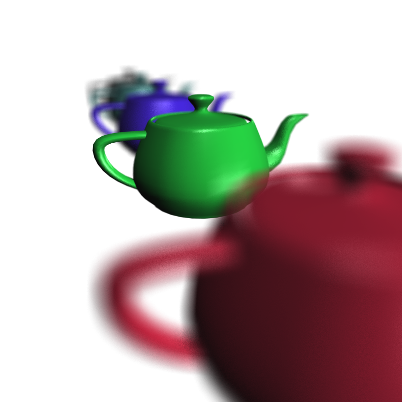
(a) Point darts, 256 per pixel.

(b) Point darts, 1024 per pixel.

(c) Line darts, 16 per pixel.

(d) Line darts, 30 per pixel.

Figure 12: Depth Of Field (DOF) images using conventional point sampling (a–b) vs. our $k$-d darts (c–d). $k$-d darts produce high-quality, antialiased images. The third column from the left shows a close up of an extremely blurry region, the Cessna’s tail. In regions close to the focal plane we see some aliasing artifacts for point darts but not for line darts, e.g. the Cessna’s prop cone, the junction of its body and wing, and the transition shades on the green teapot spout. Furthermore, line darts tend to be faster for the same quality blur; see Table 1.

4.3 Probability of Failure

Uncertainty quantification usually explores a vast high-dimensional space with a limited budget of sample points. Efficiency is crucial because typically the function evaluation is expensive and more sample points are desired than we can afford. Surrogate models create a cheaper response surface that is evaluated instead. Even for very cheap response surfaces, if the failure region is small enough Monte Carlo (MC) sampling will not estimate it accurately. Here we show that $k$-d darts can improve MC efficiency.

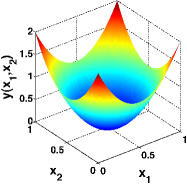
(a) Circular Parabola

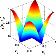
(b) Planar Cross

   

Figure 13: Plots of the two surrogate model test functions.

We test the “circular parabola” (Equation (4)) and “planar cross” (Equation (5)) surrogate models; see Figure 13.

$$y(\underline{x})=\sum_{i=1}^{d}(2x_{i}-1)^{2},\ 0<x_{i}<1.$$ (4)

$$y(\underline{x})=\left[\prod_{i=1}^{d}\frac{\left(1+\cos(2\pi x_{i})\right)}{2}\right]^{1/d},\ 0<x_{i}<1.$$ (5)

   

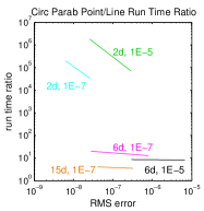
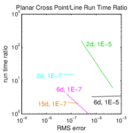
Figure 14: Speedup of line darts over point sampling for estimating the probability of failure of two analytic response surfaces.

Failure is defined as the function value below some constant threshold: $y(\underline{x})<y_{t}$. The shape of the failure region is different for the two test functions: a disk for the parabola and a fattened plus-sign for the planar cross; see Figure 13 and also Figure 1. For uniform distributions, the probability of failure is the fraction of the domain volume where $y(\underline{x})<y_{t}$. We choose $y_{t}$ so the probability of failure is exactly $10^{-5}$ or $10^{-7}$. We estimate the failure volume using line darts. For a line flat, we find the roots of the single variable equation $y(x_{i})=y_{t}$. The length of the line segment between the two roots (if real roots exist) is used to estimate the volume of the failure region. Figure 14 demonstrates the benefit of line darts over conventional point sampling in reducing the time required to achieve a given accuracy level. The complexity of root-finding reduces the performance of line darts. However, for both test functions, line darts were better than point darts in dimensions up to 15.

5 Accuracy Experiments

5.1 Problem Motivation

We provide some experimental results on the accuracy of darts for the canonical Monte Carlo problem of estimating the volume of an object in high dimensions. (Volume estimation is in the same category as the probability-of-failure problem in Section 4.3.) In particular, we seek to show that the method produces good estimates, regardless of the size, shape, dimension and orientation of the object, and regardless of the dimension and orientation of the darts. The average estimate should be close to the true estimate, and the higher moments of the estimates should be low. We design our experiments to show the effects (if any) of the following factors.

• $d$, the dimension of the object.

• $k$, the dimension of the dart. Of particular interest is comparing our results to standard MC point sampling, $k=0.$

• $s$, the squish factor of the object, which controls its aspect ratio.

• $r$, the number of rotations of the object. This allows us to compare axis-aligned objects to unaligned ones.

• Axis-aligned darts vs. unaligned darts.

We perform $N$ experiments of $n$ flats over the prior parameters, as described in Table 2. Note that we keep the number of flats constant, rather than the number of darts, because the computational expense is more closely tied to the number of flats for objects with an analytic expression, and because middle-dimensional darts have many more flats than high and low dimensional ones.

Table 2: $k$-d dart parameter study

$d$	$k$	$s$	$r$	$n$
2	0–1	${\frac{1}{10},\frac{1}{2},1,2,10}$	10	$10^{2}$–$10^{6}$
2	0–1	0.5	0, 1, 5, 10, 20	$10^{2}$–$10^{6}$
3	0–2	${\frac{1}{10},\frac{1}{2},1,\sqrt{2},\sqrt{10}}$	10	$10^{2}$–$10^{6}$
3	0–2	0.5	0, 1, 5, 10, 20	$10^{2}$–$10^{6}$
10	0–9	${\frac{1}{10},\frac{1}{2},1,\sqrt[9]{2},\sqrt[9]{10}}$	10	$10^{2}$–$10^{6}$
10	0–9	0.5	0, 1, 5, 10, 20	$10^{2}$–$10^{6}$

The darts are aligned with the coordinate axis except for some $d=2$ experiments. We repeat each parameter combination 1000 times, $N=1000$. Squish parameters $s$ are symmetric around 1 with respect to ellipse volume: e.g. for $d=2$, $s=1/2$ and $s=2$ define ellipses with the same volume.

5.2 Object Generation

Instead of a spherical object, we estimate the volume of an ellipse (a.k.a. ellipsoid), randomly oriented and squished. An ellipse provides enough generality to test the factors in Section 5.1, but enough simplicity to isolate numerical from methodology issues. In particular, we choose an ellipse because it is possible to analytically calculate the volume of an ellipse’s intersection with a $k$-d dart.

Our object is a $d$-dimensional ellipse centered at the origin. We construct it as follows. We start with a $d$-sphere centered at the origin with radius 1. This fits in an origin-centered cube with side length 2, the two-cube. We ensure the final ellipse also lies in the two-cube.

• $s$: squish factor. We scale the ellipse along the $x$-axis by multiplying its $x$-extent by $s$. The sphere has $s=1.$ Note $s<1$ gives thin, coin-shaped objects. For $s>1$, we then shrink the ellipse so it fits in the two-cube: multiply all coordinates by a factor of $1/s$. The net effect is keeping the $x$-coordinate fixed and scaling the other axes by $1/s$. This gives needle-shaped objects.

• $r$: number of rotations. We perform $r$ random rotations in sequence. Each is a Givens rotation with a random pair of coordinate indices $i$ and $j$, and a random angle $\theta\in[0,\pi]$: multiply coordinates by the identity matrix with the $2\times 2$, $\{i,j\}$ submatrix [1 0; 0 1] replaced by [$\cos{\theta}$ -$\sin{\theta}$; $\sin{\theta}$ $\cos{\theta}$].

5.3 Dart Generation

Most implementers will choose axis-aligned darts for three reasons. First, it is easy to distribute aligned darts uniformly, which ensures that the expected mean of the function estimates is accurate. Second, it is easiest to implement aligned darts, since it involves simply fixing coordinate values. Third, in many cases it is most efficient because we may obtain an expression for the underlying function along a dart by substituting in the fixed coordinate values. However, for completeness we provide some experimental results on the accuracy of unaligned darts. We shoot $k$-d darts into the two-cube as follows:

• A point dart ($k=0$) is generated by selecting a random point. Each of the $d$ coordinates is chosen independently, and uniformly in $[0,1]$.

• Aligned darts are generated by their flats. Each flat has a unique combination of $d-k$ fixed coordinate indices; the remaining $k$ coordinates are allowed to vary. The coordinates for the fixed indices are chosen independently and uniformly as for point darts.

• Unaligned flats are generated so that the orientation of the flats is uniformly random. The only experimental setting where we generate unaligned flats is for $k=1$ and $d=2$, line darts in the plane. We choose angle $\theta\in[0,\pi]$, which determines the orientation of the flat. Any line that intersects the square crosses one of its main diagonals. (It is guaranteed to cross the diagonal to which it is more perpendicular, which depends only on $\theta$.) We pick a point $p$ uniformly at random along the appropriate diagonal. We now have a point and an angle, which defines a line flat. For random darts, the second flat is a line perpendicular to the first line, passing through some random point $q$ of the other diagonal.

Aligned 1-d darts are labeled “k=1a,” random flats are labeled “k=1r,” and random darts, pairs of orthogonal flats, are labeled “k=1o” in the top two rows of Figures 15 and 16.

5.4 Object-Dart Intersection

For point darts, the volume estimation is the fraction of darts that landed inside the ellipse, multiplied by the volume of the two-cube sampling domain, $2^{d}$. For $k>0$ darts, instead of this discrete ratio we average the geometric fraction of each dart inside the ellipse object. The details of these calculations follow.

For point darts, we simply back-project the points to the domain of the sphere: apply the inverse Givens rotations to the dart’s point in reverse order; then scale the $x$-coordinate by $1/s$ (or, for $s>1$, all the other coordinates by $s$). If the distance from the transformed dart to the origin is less than 1 it is inside the sphere, and the original dart is inside the ellipse.

For $k$-d darts, we back-project their hyperplanes into the sphere domain, where we can calculate the volume of intersection analytically, and then forward-weight it by the scaling.

To back-project a flat, we back-project $k+1$ points spanning the flat. Each dart has $d-k$ fixed coordinates and $k$ free coordinates. We pick spanning point $p_{0}$ with $0$ for all of its free coordinates, and spanning point $p_{i>0}$ with 1 for its $i$th free coordinate and 0 for its other free coordinates. Each $p_{i}$ is back-projected to $q_{i}$ using the same procedure as for a point dart. The $k$ vectors from $q_{0}$ to $\{q_{i>0}\}$ span the transformed flat, but are no longer orthonormal because of the final scaling step, so we must reconstruct an orthonormal basis. Now we are ready to calculate volumes, using forward transformations. We calculate the distance from the flat to the origin. This tells us the radius of the $k$-dimensional subsphere that is the intersection of the flat with the $d$-sphere. We compute the volume of this subsphere. We multiply this volume by the sum of the $x$-components of the orthonormal basis, which gives the volume of the (unrotated) ellipse of intersection. The (forward) rotations do not affect the volume so are skipped.

For unaligned line-darts in the plane, the distance from the origin is easy to measure. We use a process similar to the prior paragraph but it is a little easier because the $1$-sphere is simply a line segment.

$d=2$, varying squish

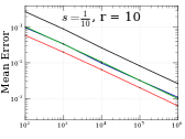
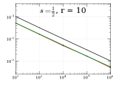
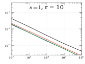
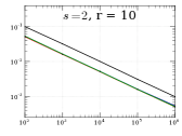
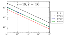
$d=2$, varying rotation

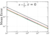
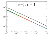
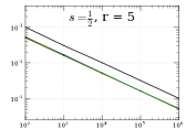
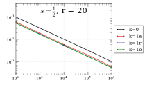
$d=3$, varying squish

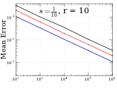
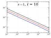
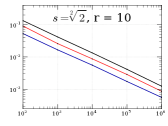
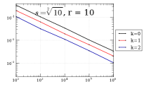
$d=3$, varying rotation

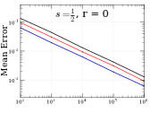
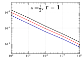
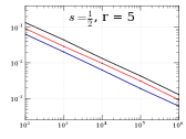
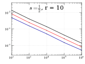
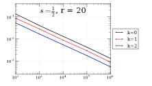
$d=10$, varying squish

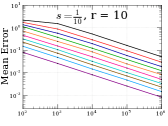
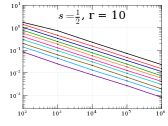
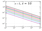
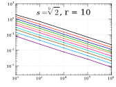
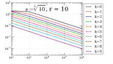
$d=10$, varying rotation

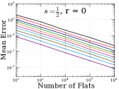
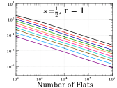
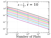
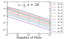
Figure 15: Mean error of volume estimation, $|\textrm{mean}-\textrm{true}|/\textrm{true}$ by $n$. See also Table 2 and Figure 16.

$d=2$, varying squish

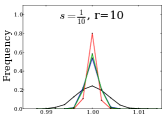
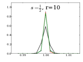
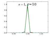
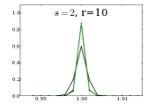
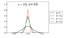
$d=2$, varying rotation

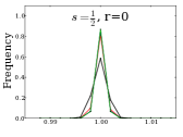
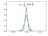
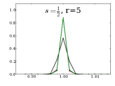
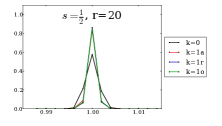
$d=3$, varying squish

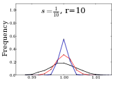
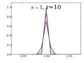
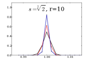
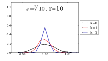
$d=3$, varying rotation

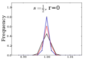
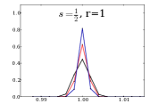
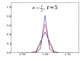
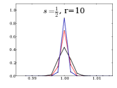
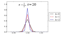
$d=10$, varying squish

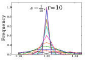
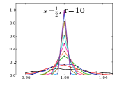
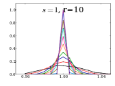
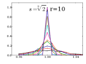
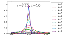
$d=10$, varying rotation

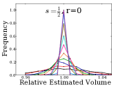
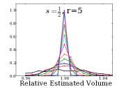
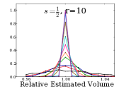
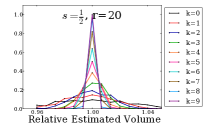
Figure 16: Volume estimation histograms, estimate / true by frequency, for $n=10^{6}.$ “1a” is axis-aligned darts, “1r” is random-angle lines, and “1o” is random-orientation darts, pairs of orthogonal flats. See also Table 2 and Figure 15.

5.5 Results

We plot the mean of the absolute value of the relative error, $|\textrm{mean}-\textrm{true}|/\textrm{true}$, vs. the number of flats $n$ in Figure 15. We plot the histograms of the ratios of estimated / true volume for $n=10^{6}$ in Figure 16. Each subfigure shows results for all $k$ for some combination of the other parameters. We observe the following.

In Figure 15 the experimental slopes for all $k$ and $d$ are about $-1/2$, in agreement with theory (the $n$ to the power $-1/2$ in Equation (1)). The accuracy is insensitive to the orientation of the object.

In Figure 16 the histograms are all sharply peaked at the true value. This shows that the variations, the higher order moments of the estimates, are reasonable.

The major trend of these figures is that the accuracy of the estimates improves with $k$. Moreover, the larger the $k$, the smaller the variation of the estimate and the sharper the peak near the true value.

For small-volume objects, aligned darts are more accurate than unaligned darts. This is illustrated by the red curves in the top-right and top-left subfigures in Figures 15 and 16. We were initially surprised by this, but the explanation is that unaligned flats are shorter on average than aligned ones, because they might clip a corner of the square rather than being the side length of the square, so they more often miss the object. (They will be even shorter as the dimension of the space increases.) For moderate-volume objects, the accuracy is about the same regardless of object orientation. For unaligned flats, it appears that our $n$ was large enough that using pairs of orthogonal flats or independently-random individual flats does not make much difference. Our conclusion is that aligned darts are universally better when the sample domain is a square.

The accuracy is primarily sensitive to the volume of the object and, secondarily, to the squish value. Higher dimensional darts are better than lower dimensional ones, and the advantage is more pronounced for small-volume objects. This can been seen by considering the second-from-bottom row in Figures 15. To see the volume dependence, note that the lines are closer together for $s=1$, and farther apart for larger and smaller squish factors. In low dimensions, 2 and 3, the smaller the volume of the object, the less accurate are all estimates, for all dimensions $k$. Moderate-dimensional darts in high dimensions, e.g. $d=10$ and $k=4$, also exhibit this trend. However, 9-d darts in 10-d space have the same accuracy regardless of the volume or squish, because they are close to the dimension of the underlying space and they more fully span it. For example, a dart with $k=d$ always evaluates to the true value. That is, the advantage of higher-dimensional darts over lower-dimensional darts is greater for small objects in high dimensions, which is where we are advocating their use.

A secondary phenomena is that the estimate is slightly more accurate for squish $s=1/10$ than for $s=\sqrt[9]{10}$, despite the volume being the same. This can be seen by careful examination of the height of the lines in the $d=10,$ varying squish row in Figure 15. For instance, the mean error is 10% lower in the first column than the fifth for $n=10^{4}$ and $k=4$. This supports our intuition that darts are effective at hitting thin, coin-shaped regions. Since $\sqrt[9]{10}\approx 1.3$, a 10-d object with this squish factor is actually roundish and not very needle-shaped. Preliminary experiments show that the accuracy gained by increasing $k$ is a complicated function of $s$ and the volume. High dimensional darts have more advantage over low dimensional ones for very small and sharp needle-shaped objects, compared to their advantage for coin-shaped objects.

6 Conclusions

In this work we introduce $k$-d darts as a conception of higher-dimensional sampling. We described a $k$-d dart framework for general dimension $k$, and then demonstrated efficiency and accuracy over three applications using using $k=1$, and accuracy for one application using $k\geq 1$. In particular, we showed that darts produce accurate estimates of the volume of an object regardless of the dimension, orientation and aspect ratio of the object. Axis-aligned darts are universally preferable to unaligned ones for sampling square domains, and we expect this to extend to hyper-rectangles, e.g. bounding boxes.

In principle, high-aspect-ratio (small-volume) objects are more efficiently sampled by higher-$k$ darts. Demonstrating that efficiency for applications requires either analytical expressions, as in the toy sphere-volume problem in the Introduction; or efficient numerical techniques for evaluating the underlying function along higher dimensional flats. In future work we plan to explore a numerical technique using recursive sampling designs by dimension.

For maximal Poisson-disk sampling, line darts are helpful in getting close to maximality in high dimensions. Below a given acceptable void ratio, they are more efficient than point darts. In terms of bounding the distance from a domain point to the nearest sample point, we are actually closer to maximality as the dimension increases. Any difference in the distribution of points produced by classical maximal Poisson-disk sampling and our line darts is small by the standard measures. Our line dart algorithm is efficient with respect to memory usage, which enables the production of larger samples in higher dimensions.

For depth-of-field, using generalized $k$-d darts gives us a high-quality noise-free image without aliasing. Although each 1-d dart requires more processing than a point sample, we only need a few of them to render a high-quality image. This results in our $k$-d dart method outperforming point sampling. We suggest sampling over a higher-dimensional space to render both depth-of-field and motion blur in animations. We suggest exploring weighted 1-d darts, where scene information determines which flats contribute more to a scene.

For uncertainty quantification, $k$-d dart Monte Carlo sampling can be more efficient than point sampling. The key for all these applications is exploiting the problem structure to take advantage of what $k$-d darts provide.

References

- [1] C. B. Barber, D. P. Dobkin, and H. T. Huhdanpaa. The quickhull algorithm for convex hulls. ACM Transactions on Mathematical Software, 22(4):469–483, 1996.
- [2] Robert L. Cook. Stochastic sampling in computer graphics. ACM Transactions on Graphics, 5(1):51–72, January 1986.
- [3] Mark A. Z. Dippé and Erling Henry Wold. Antialiasing through stochastic sampling. In Computer Graphics (Proceedings of SIGGRAPH 85), pages 69–78, July 1985.
- [4] Mohamed S. Ebeida and Scott A. Mitchell. Uniform random Voronoi meshes. In 20th International Meshing Roundtable, pages 258–275, 2011.
- [5] Mohamed S. Ebeida, Scott A. Mitchell, Anjul Patney, Andrew A. Davidson, and John D. Owens. A simple algorithm for maximal Poisson-disk sampling in high dimensions. Computer Graphics Forum, 31(2):785–794, May 2012.
- [6] Mohamed S. Ebeida, Anjul Patney, Scott A. Mitchell, Andrew Davidson, Patrick M. Knupp, and John D. Owens. Efficient maximal Poisson-disk sampling. ACM Transactions on Graphics, 30(4):49:1–49:12, July 2011.
- [7] Manuel N. Gamito and Steve C. Maddock. Accurate multidimensional Poisson-disk sampling. ACM Transactions on Graphics, 29(1):8:1–8:19, December 2009.
- [8] Peter W. Glynn and Donald L. Iglehart. Importance sampling for stochastic simulations. Management Science, 35(11):1367–1392, November 1989.
- [9] Carl Johan Gribel, Rasmus Barringer, and Tomas Akenine-Möller. High-quality spatio-temporal rendering using semi-analytical visibility. ACM Transactions on Graphics, 30:54:1–54:11, August 2011.
- [10] Carl Johan Gribel, Michael Doggett, and Tomas Akenine-Möller. Analytical motion blur rasterization with compression. In Proceedings of High Performance Graphics, pages 163–172, June 2010.
- [11] Paul E. Haeberli and Kurt Akeley. The accumulation buffer: Hardware support for high-quality rendering. In Computer Graphics (Proceedings of SIGGRAPH 90), pages 309–318, August 1990.
- [12] A. Hall. On an experimental determination of . Messenger of Mathematics, 2:113–114, 1873.
- [13] Earl Hammon Jr. Practical post-process depth of field. In Hubert Nguyen, editor, GPU Gems 3, chapter 28, pages 583–605. Addison-Wesley, 2008.
- [14] Wojciech Jarosz, Derek Nowrouzezahrai, Iman Sadeghi, and Henrik Wann Jensen. A comprehensive theory of volumetric radiance estimation using photon points and beams. ACM Transactions on Graphics, 30(1):5:1–5:19, January 2011.
- [15] Thouis R. Jones and David R. Karger. Linear-time Poisson-disk patterns. Journal of Graphics, GPU, and Game Tools, 15(3):177–182, 2011.
- [16] Thouis R. Jones and Ronald N. Perry. Antialiasing with line samples. In Proceedings of the Eurographics Workshop on Rendering Techniques 2000, pages 197–206, London, June 2000. Springer-Verlag.
- [17] Ares Lagae and Philip Dutré. A comparison of methods for generating Poisson disk distributions. Computer Graphics Forum, 27(1):114–129, March 2008.
- [18] Jaakko Lehtinen, Timo Aila, Jiawen Chen, Samuli Laine, and Frédo Durand. Temporal light field reconstruction for rendering distribution effects. ACM Transactions on Graphics, 30(4):55:1–55:12, July 2011.
- [19] Yu-Shen Liu, Jun-Hai Yong, Hui Zhang, Dong-Ming Yan, and Jia-Guang Sun. A quasi-Monte Carlo method for computing areas of point-sampled surfaces. Computer-Aided Design, 38(1):55–68, January 2006.
- [20] Nelson L. Max. Antialiasing scan-line data. IEEE Computer Graphics & Applications, 10(1):18–30, January 1990.
- [21] M. D. McKay, R. J. Beckman, and W. J. Conover. A comparison of three methods for selecting values of input variables in the analysis of output from a computer code. Technometrics, 21(2):239–245, May 1979.
- [22] Don P. Mitchell. Generating antialiased images at low sampling densities. In Computer Graphics (Proceedings of SIGGRAPH 87), pages 65–72, July 1987.
- [23] Gabriele Nebe and Neil Sloane. A catalogue of lattices. http://www.math.rwth-aachen.de/~Gabriele.Nebe/LATTICES/index.html, 2012.
- [24] A. B. Owen. A central limit theorem for Latin hypercube sampling. Journal of the Royal Statistical Society. Series B (Methodological), 54(2):541–551, 1992.
- [25] J. F. Ramaley. Buffon’s noodle problem. The American Mathematical Monthly, 76(8):916–918, October 1969.
- [26] J. Rovira, P. Wonka, F. Castro, and M. Sbert. Point sampling with uniformly distributed lines. In Proceedings of the Second Eurographics / IEEE VGTC Conference on Point-Based Graphics, SPBG’05, pages 109–118, Aire-la-Ville, Switzerland, Switzerland, 2005. Eurographics Association.
- [27] Thomas Schlömer. PSA point set analysis. http://code.google.com/p/psa/, 2011.
- [28] Jerome Spanier. Two pairs of families of estimators for transport problems. J. SIAM Appl. Math., 14:702–713, 1966.
- [29] Xin Sun, Kun Zhou, Stephen Lin, and Baining Guo. Line space gathering for single scattering in large scenes. ACM Transactions on Graphics, 29(4):54:1–54:8, July 2010.
- [30] Stanley Tzeng, Anjul Patney, Andrew Davidson, Mohamed S. Ebeida, Scott A. Mitchell, and John D. Owens. High-quality parallel depth-of-field using line samples. In Proceedings of High Performance Graphics, pages 23–31, June 2012.
- [31] Eric Veach and Leonidas J. Guibas. Metropolis light transport. In Proceedings of SIGGRAPH 97, Computer Graphics Proceedings, Annual Conference Series, pages 65–76, August 1997.
- [32] Li-Yi Wei. Parallel Poisson disk sampling. ACM Transactions on Graphics, 27(3):20:1–20:9, August 2008.
- [33] Kenric B. White, David Cline, and Parris K. Egbert. Poisson disk point sets by hierarchical dart throwing. In RT ’07: Proceedings of the 2007 IEEE Symposium on Interactive Ray Tracing, pages 129–132, September 2007.