A complicated Duffing oscillator in the surface-electrode ion trap

Abstract

The oscillation coupling and different nonlinear effects are observed in a single trapped ${}^{40}Ca^{+}$ ion confined in our home-built surface-electrode trap (SET). The coupling and the nonlinearity are originated from the high-order multipole potentials due to different layouts and the fabrication asymmetry of the SET. We solve a complicated Duffing equation with coupled oscillation terms by the multiple scale method, which fits the experimental values very well. Our investigation in the SET helps for exploring nonlinearity using currently available techniques and for suppressing instability of qubits in quantum information processing with trapped ions.

I introduction

The Duffing oscillator is generally used to describe nonlinear dynamics in oscillating systems Nayfeh1979 ; M.I. Dykman ; L. D. Landau ; Nayfeh1981 . The corresponding Duffing equation models a damping and driven oscillator with more complicated behavior than simple harmonic motion, which can be used to exhibit chaos in dynamics and hysteresis in resonance V. I. Arnold ; S. H. Strogatz ; H. B. Chan ; M. I. Dylman2004 ; B. Yurke ; E. Buks .

On the other hand, the motion of trapped ions is highly controllable and can be employed to transfer quantum information when cooled down to ground state blatt . Since it is effectively approximated to be harmonic, the ion motion in a quadruple electromagnetic trap W. Paul can be regarded as a good mechanical oscillator, which may exhibit nonlinearity when driven to the nonlinear field. For example, Duffing nonlinear dynamics has been investigated in a single ion confined in the linear ion trap aker . The trap nonlinearity introduces instability in the motion of the ion, which should be avoided in most times, but can also be used in resonance rejection and parameter detection in mass spectrometry mak ; dra . Recent research also showed the feasibility of phonon lasers based on the nonlinearity of a single trapped ion under laser irradiation vahala .

We focus in this work on the nonlinearity in a home-built surface-electrode trap (SET). The SET, with capability to localize and transport trapped ions in different potential wells, is a promising setup for large-scale quantum information processing wineland . In comparison to conventional linear Paul traps, however, the reduced size and asymmetry in SET lead to stronger high-order multipole potentials wesen ; house ; Blakestad , which affect the stability of the ion trapping. To solve the problem we have to understand the source and the strength of the nonlinearity. Due to complexity resulted from the high-order multipole potentials, the nonlinear effect in the SET cannot be simply described by the Duffing oscillator as for the linear trap, but an inhomogeneous-coupled Duffing oscillator involving quadratic and cubic nonlinearities. We observed the nonlinearity experimentally in our SET, and by the method of multiple scales we derived an inhomogeneous-coupled Duffing oscillator to fit the experimental values, which shows that both the nonlinearity and axial-radial coupling exist in the case of the frequency resonance (i.e., around the regime of driving detuning being zero). Moreover, we show in the non-coupling case different nonlinear effects in different dimensions, which is due to different asymmetry in fabrication of the SET.

II experimental setup and images of ion motion

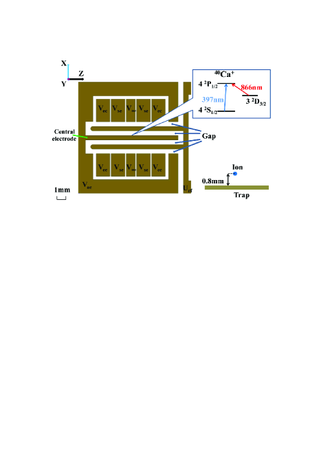
Figure 1: The layout of our home-built SET with the top-right inset for the relevant energy levels of the trapped ${}^{40}Ca^{+}$ ion. The ${}^{40}Ca^{+}$ ion is cooled by the laser beam at 397 nm on the $4s^{2}S_{1/2}\longleftrightarrow 4p^{2}P_{1/2}$ transition, helped by another laser light at 866 nm as repumping. Here, the trapped ion is above the electrodes by 0.8 mm (See the bottom-right inset).

Our home-built SET is a 500 $\mu$m-scaled planar trap with five electrodes for radial confinement, and fabricated by printed circuit board technology chip . As shown in Fig. 1, the five electrodes consists of a central electrode, two radio-frequency (rf) electrodes and two outer segmented dc electrodes, where the rf electrodes, the central electrode and the gaps in between are of the same width of 500 $\mu$m. Each outer segmented electrode consists of five component electrodes, i.e., a middle electrode, two control electrodes and two end electrodes. The widths of the control electrodes and end electrodes in the segment are 1.5 mm and the middle electrode is 1 mm wide. The gap in the segmented electrode is of 500 $\mu$m width. When the SET works, the trapped ${}^{40}Ca^{+}$ ion stays above the electrodes by $0.8$ mm, and the pseudopotential trapping depth is below $1$ eV with rf amplitude $U$(0-peak)$=400$ V and rf frequency $\Omega/2\pi=15$ MHz. The voltage on the four end electrodes is $V_{ec}=40$ V but zero on other electrodes.

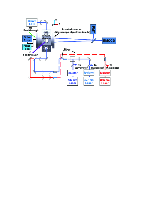
Figure 2: Schematic of our experimental setup. The main components are explained in the text.

The experimental setup is plotted in Fig. 2, where the ultraviolet radiation at $397$ nm excites $4s^{2}S_{1/2}\longleftrightarrow 4p^{2}P_{1/2}$ transition by a grating stabilized laser diode with power up to $30$ mW and linewidth less than 2 MHz. Another grating stabilized laser diode at $866$ nm with power up to 100 mW and linewidth less than 5 MHz excites the $3d^{2}D_{3/2}\longleftrightarrow 4p^{2}P_{1/2}$ transition. The frequencies of the both laser diodes have been calibrated to the wavelength meter (HighFiness, WS-7). Typical laser powers at the trap center are 50 $\mu$W for 397 nm in red detuning (-80 MHz) and 500 $\mu$W for 866 nm in carrier transition. In our SET, the single ${}^{40}Ca^{+}$ ion is laser cooled and stably confined, which is monitored by photon scattering collected by both an electron-multiplying charge-coupled-device (EMCCD) camera and a photomultiplier tube (PMT). Outside the vacuum chamber, the electrical connections immediately encounter a ”filter box”, which provides low-pass filtering of the voltages applied to the electrode. An additional drive force is electrically connected to one of the middle electrodes behind the filter box, which provides an excitation to drive the ion away from equilibrium. Due to the design of our SET system, the motion of the ion is detected only in the $xz$ plane by the EMCCD. As a result, what we study throughout the work is the oscillation along the axial direction ($z$-axis) and the radial direction ($x$-axis), whose harmonic frequencies are, respectively, $\omega_{0z}/2\pi=191.7$ kHz and $\omega_{0x}/2\pi=425$ kHz. Moreover, since the harmonic frequency in $y$-axis is $\omega_{0y}/2\pi=925$ kHz, much bigger than in other axes, the ion can be regarded as a very tight confinement in y direction. We have suppressed the micro-motion by the rf-photon cross correlation compensation njp , which yield cooling of the ion down to the temperature below 10 mK.

To study the nonlinear mechanical response, we drive the ion to the nonlinear regime by a small oscillating voltage, i.e., $V=7$ V, applied to one of the middle electrodes. We slowly increase the driving frequency with the scan step $0.1$ kHz, from $189.0$ kHz to $433.0$ kHz (the positive scan), the ion oscillates first along the $z$-axis and then turns to the $x$-axis for oscillation. The particularly interesting observation is the simultaneous responses, i.e., a rectangle trajectory, in both $x$- and $z$- axes when the sweep is close to the harmonic resonator frequency in either of the axes. Similar behavior is also found in the negative scan.

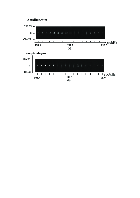
Figure 3: Time-averaged images of a single trapped ion taken at different drive frequencies, with (a) the positive scan and (b) the negative scan. The prime oscillation is along the axial direction and the scan step is 0.1 kHz. The rectangles appear in the images at resonance frequency due to axial-radial coupling.

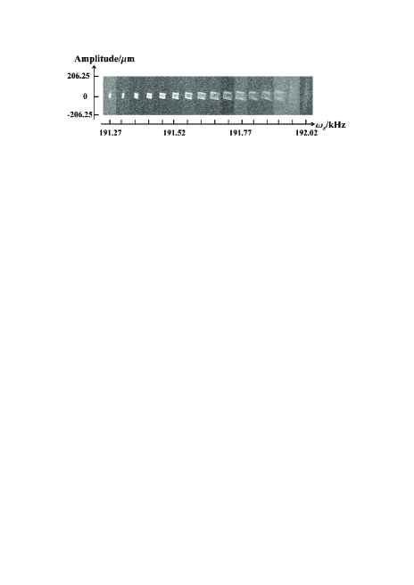
Figure 4: The coupled oscillation in the time-average images for the positive scan. Comparing to Fig. 3, the scan with smaller step (0.01 kHz) presents clearer pictures for the rectangle trajectories from appearance to disappearance, where sixteen images are selected in series with the frequency step 0.05 kHz.

We measure the ion oscillation by taking time-averaged images from the EMCCD. In Fig. 3, seventeen such images for different drive frequencies are presented for positive and negative scans, respectively. For the ion originally oscillating in the $z$-axis, we slowly scan the drive frequency $\omega_{z}$ across the harmonic resonance at $\omega_{0z}$. When the detuning $\sigma=\omega_{z}-\omega_{0z}$ approaches zero, the rectangle trajectory appears, implying a coupled motion between $x$- and $z$-axes due to axial-radial coupling (explained later). For a more clarified observation, we scan with smaller steps around the regime $\sigma=0$, as shown in Fig. 4 which gives us an accurate range from the appearance of the rectangle to the disappearance.

III theoretical model

To understand the observation above, we have to consider the multipole potential in the SET, which is given by Littich

$$\phi_{i}\left(x,y,z\right)=\sum_{j=1}^{\infty}g_{ij}M_{j}Y_{j}\left(x,y,z\right),$$ (1)

where the subscript $i$ labels different electrodes and the subscript $j$ is for the spherical harmonics $Y_{j}\left(x,y,z\right)$. Both $Y_{j}\left(x,y,z\right)$ and the related parameters $M_{j}$ are defined in Littich . $g_{ij}$ is the weight factor for different electrodes. In this treatment, the initial equilibrium position of the single trapped ion is defined as the origin of the coordinates. The five-wire SET generally consists of quadrupole and hexapole potentials Blakestad . Considering the defect in our SET, we also involve octopole potential in our treatment. Following the definition in Littich , we have the subscripts $j=5,\cdots,25$ where $j$ from 5 to 9, from 10 to 16 and from 17 to 25 correspond, respectively, to the quadrupole, hexapole and octopole potentials. For different potentials $\Psi_{i}=V_{i}+U_{i}\cos(\Omega t)$ applied, respectively, to N electrodes, where $V_{i}$ is the dc voltage on the electrode $i$ and $U_{i}\cos(\Omega t)$ represents the rf voltage $U_{i}$ on the electrode $i$ driven at frequency $\Omega$, we rewrite Eq. (1) for the dc potential $\Phi_{dc}$ and the rf potential $\Phi_{rf}$ as

$$\begin{array}[]{c}\Phi_{dc}\left(x,y,z\right)=\sum_{j=5}^{25}V_{j}^{\ast}M_{j}Y_{j}\left(x,y,z\right),\\ \Phi_{rf}\left(x,y,z\right)=\sum_{j=5}^{25}U_{j}^{\ast}\cos(\Omega t)M_{j}Y_{j}\left(x,y,z\right),\end{array}$$ (2)

where we have used $U_{j}^{\ast}=\sum_{i=1}^{N}U_{i}g_{ij}$ and $V_{j}^{\ast}=\sum_{i=1}^{N}V_{i}g_{ij}$.

Moreover, we have the 1D motional equation for the trapped ion Doroudi ,

$$\frac{d^{2}\xi}{dt^{2}}+2\mu\frac{d\xi}{dt}+\frac{e}{m}\frac{\partial\Phi_{dc}}{\partial\xi}+\frac{e^{2}}{2m^{2}}\frac{\partial}{\partial\xi}\left(\left\langle\left|\int\frac{\partial\Phi_{rf}}{\partial\xi}dt\right|^{2}\right\rangle\right)$$ (3)

$$= k_{\xi}\cos(\omega_{\xi}t),$$

with $\xi=x,y$ and $z$. Combining Eq. (2) with Eq. (3), we obtain the equation of motion in the $z$ direction,

$$\begin{array}[]{c}\frac{d^{2}z}{dt^{2}}+2\mu\frac{dz}{dt}+\omega_{0z}^{2}z+\alpha_{2}z^{2}+\alpha_{3}z^{3}+\alpha_{21}z^{2}y+\alpha_{22}z^{2}x\\ +\alpha_{4}zy^{2}+\alpha_{5}zx^{2}+\alpha_{6}zxy+\alpha_{7}zy+\alpha_{8}zx=k_{z}\cos(\omega_{z}t),\end{array}$$ (4)

where $x$, $y$ and $z$ represent, respectively, the displacement of the ion from the equilibrium position in the three dimensions, $\mu$ is the linear damping parameter originated from the recoil due to photon absorption, $k_{z}$ is driving amplitude. The detailed expressions of the nonlinear coefficients $\alpha_{i}$ $(i=2,21,22,3,4,5,6,7,8)$ can be found in Appendix I. Compared to the Duffing oscillator in aker , Eq. (4) is a complicated Duffing oscillator, containing additional coupled-motion terms.

Using the method of multiple scales S.S2001 , we obtain the steady-state solution to Eq. (4) as

$$\sigma = \frac{3a^{2}}{8\omega_{0z}}(\alpha_{3}+\frac{-10\alpha_{2}^{2}}{9\omega_{0z}^{2}}+\frac{-2\alpha_{8}\alpha_{2x}c^{2}}{3\omega_{0x}^{2}a^{2}}+\frac{-2\alpha_{7}\alpha_{2y}b^{2}}{3\omega_{0y}^{2}a^{2}}$$ (5)

$$+\frac{2\alpha_{4}b^{2}}{3a^{2}}+\frac{2\alpha_{5}c^{2}}{3a^{2}})\pm\sqrt{\frac{k_{z}^{2}}{4\omega_{0z}^{2}a^{2}}-\mu^{2}},$$

where the nonlinear coefficients $\alpha_{2x}$ and $\alpha_{2y}$ are relevant to the coupled motion along $x$- and $y$-axes. $c$, $b$ and $a$ are the response amplitudes, respectively, in $x$, $y$ and $z$ directions. $\omega_{0x}/2\pi$ and $\omega_{0y}/2\pi$ represent the harmonic frequencies in $x$- and $y$-axes. For more clarification, we define a parameter $\alpha_{total}$ as

$$\alpha_{total}=\alpha_{3}+\Delta\alpha_{2}+\Delta\alpha,$$ (6)

where $\alpha_{3}$ originates from the cubic nonlinearity, $\Delta\alpha_{2}=\frac{-10\alpha_{2}^{2}}{9\omega_{0z}^{2}}$ represents the nonlinear coefficient that comes from quadric nonlinearity, and $\Delta\alpha=\frac{-2\alpha_{8}\alpha_{2x}c^{2}}{3\omega_{0x}^{2}a^{2}}+\frac{-2\alpha_{7}\alpha_{2y}b^{2}}{3\omega_{0y}^{2}a^{2}}+\frac{2\alpha_{4}b^{2}}{3a^{2}}+\frac{2\alpha_{5}c^{2}}{3a^{2}}$ corresponds to the nonlinear dispersion relevant to the coupled motion. Substituting $\alpha_{total}$ into Eq. (5), we obtain

$$\sigma=\frac{3\alpha_{total}}{8\omega_{0z}}a^{2}\pm\sqrt{\frac{k_{z}^{2}}{4\omega_{0z}^{2}a^{2}}-\mu^{2}}.$$ (7)

IV discussion about the nonlinearity and coupling

In our home-built SET, since the harmonic frequency in y-axis is much bigger than in other axes, the ion is confined very tightly in y direction, which leads to a reasonable assumption $b/a\ll$1. As a result, the coupled term $\Delta\alpha$ is reduced to $\Delta\alpha=\chi c^{2}/a^{2}$ with $\chi=\frac{-2\alpha_{8}\alpha_{2x}}{3\omega_{0x}^{2}}+\frac{2\alpha_{5}}{3}$. Moreover, $\alpha_{3}$ and $\Delta\alpha_{2}$ in Eq. (6) are nothing to do with the coupled motion and their sum $\alpha_{3}+\Delta\alpha_{2}$ can be measured experimentally by

$$a_{m}=\sqrt{\frac{8\omega_{0z}\sigma_{m}}{3(\alpha_{3}+\Delta\alpha_{2})}},$$ (8)

with the maximal amplitude $a_{m}$ and the maximal detuning $\sigma_{m}$ in the non-coupling case. As a result, Eq. (7) is reduced to a steady-state solution to the amplitude of the response $a$ with respect to the drive detuning $\sigma$ for the known driving force amplitude $k_{z}$,

$$\sigma=\frac{3a^{2}}{8\omega_{0z}}(\alpha_{3}+\Delta\alpha_{2}+\chi\frac{c^{2}}{a^{2}})\pm\sqrt{\frac{k_{z}^{2}}{4\omega_{0z}^{2}a^{2}}-\mu^{2}}.$$ (9)

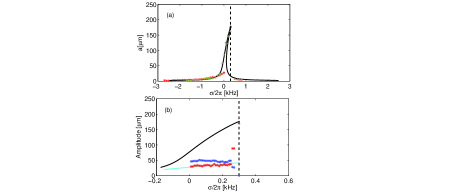
Figure 5: The measured and calculated amplitudes with respect to the driving detuning, where the black dashed lines indicate the detunings for maximum amplitudes of oscillations. (a) The measured values correspond to the situation in Fig. (3). Calculation (black solid curve) by Eq. (9) without the coupling term fits most of the measured values with positive scan (red stars) and negative scan (green crosses). The scan step is $0.1$ kHz. (b) The measured values correspond to the situation in Fig. (4). Calculation (light blue solid line) by Eq. (9) with the coupling term fits the measured values with positive slow scan (red stars) around zero detuning. The scan step is $0.01$ kHz, and the blue stars are for the measured values of the vibrational amplitude $c$ in $x$-axis. As a comparison, the calculation without the coupling term is plotted (the black solid curve).

In our experiment, $\omega_{0z}$ is measured via ion response in the linear regime, $k_{z}=0.075\times 10^{6}$ Hz²m is obtained by observing the ion displacement versus the middle electrode voltage house , $\alpha_{3}+\Delta\alpha_{2}=0.1959\times 10^{18}$ Hz ²/m² is measured using the observed dependence of $a_{m}$ on the maximal detuning $\sigma_{m}$. We evaluate $\mu=177.1$ Hz using the relation $a_{m}=k_{z}/\left(2\mu\omega_{0z}\right)$. The comparison in the non-coupling case between the measured and calculated values of $a$ and $\sigma$ is made in Fig. 5(a), where Eq. (9) without the coupling term $\Delta\alpha$ (the black solid curve) can fit most experimental values for both the positive and negative scans (red stars and green crosses, respectively). In this situation, the vibrational amplitude $c$ in $x$-axis is negligible. Some experimental values around $\sigma=0$, which are not fitted well by the solid curve, are actually relevant to the case of coupled motion. To be more clarified, we scan the region around $\sigma=0$ with smaller step than in Fig. 5(a). The fitting by considering the coupling term $\Delta\alpha$ in our calculation can fully cover the measured data, as shown in Fig. 5(b). In such a case, we find that the vibrational amplitude $c$ in $x$-axis is visible, which is excited by the energy transfer from $z$-axis due to motional coupling. This energy transferred from $z$-axis to $x$-axis is nearly constant in the adiabatic operation so that we obtain $\chi\frac{c^{2}}{a^{2}}\approx 4.5\times 10^{18}$ Hz²/m². Fig. 5(b) also shows that the motional coupling stops when $\sigma/2\pi$ approaches $0.25$ kHz. We see that $a$ goes up to a maximum with $c$ dropping to zero, implying that the system returns to the non-coupling case. Therefore, the vibrational trajectories imaged in Figs. 3 and 4 can be fully understood by the complicated Duffing oscillator with and without the term for coupled motion.

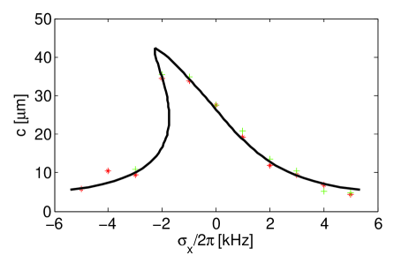
Figure 6: The measured and calculated amplitudes in $x$-axis with respect to the driving detuning, where the scan step is 1 kHz and the measurement is made in the no-coupling case. Calculation (black solid curve) fits most of the measured values with positive scan (red stars) and negative scan (green crosses).

Moreover, we also checked nonlinear effects in different directions in our SET by applying the drive on the $x$-axis and repeating the experimental steps as above for $z$-axis. It is physically evident that the behavior can be described by a slight modification of Eq. (4) by exchanging $z$ and $x$, and replacing $k_{z}$ and $\omega_{z}$ by $k_{x}$ and $\omega_{x}$. As an example, we only present the non-coupling case in Fig. 6, where the measured data is fitted well by the steady solution to the complicated Duffing oscillator with different nonlinear coefficients and different damping rates from in Fig. 5(a). In comparison to the shape of the curve in Fig. 5(a), the oscillation in such a case reaches the maximum amplitude before $\sigma=0$, i.e, the red detuning, corresponding to $\alpha_{3}+\Delta\alpha_{2}<0$ in Eq. (8). This implies negative coefficients of quadratic and cubic terms in Eq. (4) originated from the different asymmetry from in $z$-axis.

V conclusion

In conclusion, we have experimentally investigated the complicated oscillations in our home-built SET, which are related to the high-order multipole potentials. Both the coupling and non-coupling cases, as well as the driving along different axes, are studied. Our observation can be fully understood by the nonlinear effects and the motional coupling from the solution of a complicated Duffing oscillator.

In comparison to the relevant study on a single ion oscillating in the linear trap aker , our home-made SET owns higher-order multipole potentials, which cause more fruitful nonlinear effects and even the motional coupling between different directions. Although there are also axial-radial couplings observed in the ion trap, e.g., with ion cloud in cloud , such a motional coupling is much more evident in the SET, which, in addition to the couplings regarding $zx$ and $xz^{2}$, is also reflected in the $zx^{2}$ term in Eq. (4) with the coefficient $\alpha_{5}$. According to our calculation, the motional coupling in our observation is mainly influenced by the coefficients $\alpha_{5}$ and $\alpha_{8}$, which implies the combined action from the quadrupole, hexapole and octopole potentials. This is the reason that the rectangle trajectories have never been observed previously in linear ion traps. Moreover, recent investigation of the phonon laser based on the nonlinear oscillation of the trapped ion demonstrated the analogy to the Fabry-Perot laser with 100% reflecting mirrors vahala . In contrast, the SET under our study seems an asymmetry Fabry-Perot cavity, which may yield two split beams of the phonon laser in perpendicular axes. Coherent transfer between the two split phonon beams would be useful in fundamental physics and practical application. Further work in this aspect is underway.

With the trapped ions cooled down to the motional ground state, we may have an excellent platform to demonstrate nonlinear behavior in a fully quantum mechanical regime and also carry out quantum logic gate operations. Therefore our work presents a way to exploring complicated nonlinearity using experimentally available techniques and it is also useful for suppressing detrimental effects from the nonlinearity in quantum information processing using trapped ions.

Appendix I     The nonlinear coefficients in Eq. (4)

Our calculation is based on Eq. (4), in which the nonlinear coefficients originate from the high-order multipole potentials. By setting $e$ and $m$ to be the electric quantity and the mass of single calcium ion, we have the nonlinear coefficients as

$$\alpha_{3}=\frac{36e^{2}r_{0}^{2}\left(U_{13}^{\ast}\right)^{2}M_{13}^{2}}{m^{2}r_{0}^{8}\Omega^{2}}+\frac{140eM_{21}\left[mr_{0}^{4}(V_{21}^{\ast})\Omega^{2}+8er_{0}^{2}\left(U_{21}^{\ast}\right)\left(U_{7}^{\ast}\right)M_{7}\right]}{m^{2}r_{0}^{8}\Omega^{2}},$$ (10)

$$\alpha_{2}=\frac{6er_{0}M_{13}\left[mr_{0}^{4}(V_{13}^{\ast})\Omega^{2}+6er_{0}^{2}\left(U_{7}^{\ast}\right)\left(U_{13}^{\ast}\right)M_{7}\right]}{m^{2}r_{0}^{8}\Omega^{2}},$$ (11)

$$\alpha_{21} = \frac{3e\left[70er_{0}^{2}M_{6}M_{21}(U_{6}^{\ast})(U_{21}^{\ast})+42er_{0}^{2}M_{7}M_{20}(U_{7}^{\ast})(U_{20}^{\ast})\right]}{m^{2}r_{0}^{8}\Omega^{2}}$$ (12)

$$+\frac{3e\left[24er_{0}^{2}M_{12}M_{13}(U_{12}^{\ast})(U_{13}^{\ast})+7mr_{0}^{4}\Omega^{2}M_{20}(V_{20}^{\ast})\right]}{m^{2}r_{0}^{8}\Omega^{2}},$$

$$\alpha_{22} = \frac{3e\left[70er_{0}^{2}M_{8}M_{21}(U_{8}^{\ast})(U_{21}^{\ast})+42er_{0}^{2}M_{7}M_{22}(U_{7}^{\ast})(U_{22}^{\ast})\right]}{m^{2}r_{0}^{8}\Omega^{2}}$$ (13)

$$+\frac{3e\left[24er_{0}^{2}M_{13}M_{14}(U_{13}^{\ast})(U_{14}^{\ast})+7mr_{0}^{4}\Omega^{2}M_{22}(V_{22}^{\ast})\right]}{m^{2}r_{0}^{8}\Omega^{2}},$$

$$\alpha_{4} = \frac{e\left[32er_{0}^{2}\left(U_{12}^{\ast}\right)^{2}M_{12}^{2}-18er_{0}^{2}\left(U_{13}^{\ast}\right)^{2}M_{13}^{2}-6er_{0}^{2}\left(U_{13}^{\ast}\right)\left(U_{15}^{\ast}\right)M_{13}M_{15}+21er_{0}^{2}\left(U_{6}^{\ast}\right)\left(U_{20}^{\ast}\right)M_{6}M_{20}\right]}{m^{2}r_{0}^{8}\Omega^{2}}$$ (14)

$$+\frac{e\left[-60mr_{0}^{4}(V_{21}^{\ast})\Omega^{2}M_{21}-14mr_{0}^{4}(V_{23}^{\ast})\Omega^{2}M_{23}-240er_{0}^{2}(U_{7}^{\ast})\left(U_{21}^{\ast}\right)M_{7}M_{21}-56er_{0}^{2}(U_{7}^{\ast})\left(U_{23}^{\ast}\right)M_{7}M_{23}\right]}{m^{2}r_{0}^{8}\Omega^{2}},$$

$$\alpha_{5} = \frac{e\left[32er_{0}^{2}\left(U_{14}^{\ast}\right)^{2}M_{14}^{2}-18er_{0}^{2}\left(U_{13}^{\ast}\right)^{2}M_{13}^{2}+6er_{0}^{2}\left(U_{13}^{\ast}\right)\left(U_{15}^{\ast}\right)M_{13}M_{15}+21er_{0}^{2}M_{8}M_{22}(U_{8}^{\ast})(U_{22}^{\ast})\right]}{m^{2}r_{0}^{8}\Omega^{2}}$$ (15)

$$+\frac{e\left[-60mr_{0}^{4}(V_{21}^{\ast})\Omega^{2}M_{21}+14mr_{0}^{4}(V_{23}^{\ast})\Omega^{2}M_{23}-240er_{0}^{2}(U_{7}^{\ast})\left(U_{21}^{\ast}\right)M_{7}M_{21}+56er_{0}^{2}(U_{7}^{\ast})\left(U_{23}^{\ast}\right)M_{7}M_{23}\right]}{m^{2}r_{0}^{8}\Omega^{2}},$$

$$\alpha_{6} = \frac{e\left[6er_{0}^{2}\left(U_{13}^{\ast}\right)\left(U_{11}^{\ast}\right)M_{13}M_{11}+14mr_{0}^{4}(V_{19}^{\ast})\Omega^{2}M_{19}+21er_{0}^{2}\left(U_{6}^{\ast}\right)\left(U_{22}^{\ast}\right)M_{6}M_{22}\right]}{m^{2}r_{0}^{8}\Omega^{2}}$$ (16)

$$+\frac{e\left[64er_{0}^{2}(U_{12}^{\ast})\left(U_{14}^{\ast}\right)M_{12}M_{14}+56er_{0}^{2}\left(U_{7}^{\ast}\right)\left(U_{19}^{\ast}\right)M_{7}M_{19}+21er_{0}^{2}M_{8}M_{20}(U_{8}^{\ast})(U_{20}^{\ast})\right]}{m^{2}r_{0}^{8}\Omega^{2}},$$

$$\alpha_{7}=\frac{e\left[6er_{0}^{3}\left(U_{13}^{\ast}\right)\left(U_{6}^{\ast}\right)M_{13}M_{6}+8mr_{0}^{5}(V_{12}^{\ast})\Omega^{2}M_{12}+32er_{0}^{3}\left(U_{12}^{\ast}\right)\left(U_{7}^{\ast}\right)M_{12}M_{7}\right]}{m^{2}r_{0}^{8}\Omega^{2}},$$ (17)

$$\alpha_{8}=\frac{e}{m^{2}r_{0}^{8}\Omega^{2}}\left[8mr_{0}^{5}(V_{14}^{\ast})\Omega^{2}M_{14}+32er_{0}^{3}\left(U_{14}^{\ast}\right)\left(U_{7}^{\ast}\right)M_{14}M_{7}+6er_{0}^{3}M_{8}M_{13}(U_{8}^{\ast})(U_{13}^{\ast})\right],$$ (18)

with $\omega_{0z}^{2}=e\left[8er_{0}^{4}\left(U_{7}^{\ast}\right)^{2}M_{7}^{2}+4mr_{0}^{6}(V_{7}^{\ast})\Omega^{2}M_{7}\right]/m^{2}r_{0}^{8}\Omega^{2}$, and the scaling factor $r_{0}$ (See definition in Littich ).

Appendix II     Details of the steady-state solution Eq. (5)

Eq. (5) is obtained by the standard steps of the multiple scale method. Starting from Eq. (4), we assume that the driving frequency is a perturbative expansion of harmonic oscillator frequency Nayfeh1985 , i.e., $\omega_{z}=\omega_{0z}+\epsilon^{2}\sigma$, with a small dimensionless parameter $\epsilon$. Following the method in Nayfeh1984 , we rewrite Eq. (4) by setting $z=\epsilon u$, $x=\epsilon p$, $y=\epsilon q$, the damping term as $2\epsilon^{3}\mu\dot{u}$ and the driving term as $\epsilon^{3}k_{z}\cos(\omega_{z}t)$. Introducing a new parameter $T_{i}=\epsilon^{i}t$ $(i=0,1,2)$, we rewrite $u,p,q$ as,

$$\begin{array}[]{c}u=\epsilon^{0}u_{0}\left(T_{0},T_{1},T_{2}\right)+\epsilon^{1}u_{1}\left(T_{0},T_{1},T_{2}\right)+\epsilon^{2}u_{2}\left(T_{0},T_{1},T_{2}\right),\\ p=\epsilon^{0}p_{0}\left(T_{0},T_{1},T_{2}\right)+\epsilon^{1}p_{1}\left(T_{0},T_{1},T_{2}\right)+\epsilon^{2}p_{2}\left(T_{0},T_{1},T_{2}\right),\\ q=\epsilon^{0}q_{0}\left(T_{0},T_{1},T_{2}\right)+\epsilon^{1}q_{1}\left(T_{0},T_{1},T_{2}\right)+\epsilon^{2}q_{2}\left(T_{0},T_{1},T_{2}\right).\end{array}$$ (19)

Then we compare the coefficients of $\epsilon^{0}$, $\epsilon^{1}$ and $\epsilon^{2}$, which yields,

$$D_{0}^{2}u_{0}+\omega_{0z}^{2}u_{0}=0,$$ (20)

$$D_{0}^{2}u_{1}+\omega_{0z}^{2}u_{1}=-2D_{0}D_{1}u_{0}-\alpha_{2}u_{0}^{2}-\alpha_{7}q_{0}u_{0}-\alpha_{8}p_{0}u_{0},$$ (21)

$$D_{0}^{2}u_{2}+\omega_{0z}^{2}u_{2} = -[-k_{z}\cos\left(\omega_{0z}T_{0}+\sigma T_{2}\right)+q_{0}^{2}\alpha_{4}u_{0}+p_{0}^{2}\alpha_{5}u_{0}+p_{0}q_{0}\alpha_{6}u_{0}+2\mu D_{0}u_{0}$$ (22)

$$+D_{1}^{2}u_{0}+2D_{0}D_{2}u_{0}+q_{0}\alpha_{21}u_{0}^{2}+p_{0}\alpha_{22}u_{0}^{2}+\alpha_{3}u_{0}^{3}+2D_{0}D_{1}u_{1}$$

$$+\alpha_{7}q_{0}u_{1}+\alpha_{8}p_{0}u_{1}+2\alpha_{2}u_{0}u_{1}+\alpha_{7}q_{1}u_{0}+\alpha_{8}p_{1}u_{0}],$$

where $D_{i}=\partial/\partial T_{i}$, $\left(i=0,1,2\right)$.

We may solve $u_{0}=A\left(T_{2}\right)\exp(i\omega_{0z}T_{0})+\bar{A}\left(T_{2}\right)\exp(-i\omega_{0z}T_{0})$ and $u_{1}=\alpha_{2}[A^{2}\exp(2i\omega_{0z}T_{0})-6A\bar{A}+\bar{A}^{2}\exp(-2i\omega_{0z}T_{0})]/3\omega_{0z}^{2}$ from Eqs. (20) and (21) by eliminating the secular term. Similarly, from equations of the oscillations in x-axis and y-axis, we may solve the variables $p_{0}$, $q_{0}$, $p_{1}$ and $q_{1}$ as

$$p_{0}=C\left(T_{2}\right)\exp(i\omega_{0x}T_{0})+\bar{C}\left(T_{2}\right)\exp(-i\omega_{0x}T_{0}),$$ (23)

$$q_{0}=B\left(T_{2}\right)\exp(i\omega_{0y}T_{0})+\bar{B}\left(T_{2}\right)\exp(-i\omega_{0y}T_{0}),$$ (24)

$$p_{1}=\alpha_{2x}[C^{2}\exp(2i\omega_{0x}T_{0})-6C\bar{C}+\bar{C}^{2}\exp(-2i\omega_{0x}T_{0})]/(3\omega_{0x}^{2}),$$ (25)

$$q_{1}=\alpha_{2y}[B^{2}\exp(2i\omega_{0y}T_{0})-6B\bar{B}+\bar{B}^{2}\exp(-2i\omega_{0y}T_{0})]/(3\omega_{0y}^{2}),$$ (26)

where $\alpha_{2x}$ and $\alpha_{2y}$ correspond to the quadric nonlinearity of the ion motion equation in $x$ and $y$ directions, respectively. $\omega_{0x}/2\pi$ and $\omega_{0y}/2\pi$ represent the harmonic frequencies in x direction and y direction. $A=\frac{1}{2}a\exp(i\beta)$, $B=\frac{1}{2}b\exp(i\varsigma)$ and $C=\frac{1}{2}c\exp(i\eta)$, where $a,b,c,\beta,\varsigma$ and $\eta$ are real functions of $T_{2}$, $\beta,\varsigma$ and $\eta$ represent the phases of different dimensions. $\bar{A}$, $\bar{B}$ and $\bar{C}$ are conjugate terms of A, B and C. Substituting $u_{0}$ and $u_{1}$ into Eq. (22), we obtain an equation regarding the secular term, from which, in combination of Eqs. (23-26) with the expressions of $A$, $B$ and $C$, we obtain

$$-\frac{1}{2}k_{z}\sin\gamma+a\mu\omega_{0z}+\omega_{0z}\frac{da}{dT_{2}}=0,$$ (27)

$$\frac{1}{2}k_{z}\cos\gamma-\frac{3\alpha_{3}a^{3}}{8}-\frac{1}{4}\alpha_{4}ab^{2}-\frac{1}{4}\alpha_{5}ac^{2}+\frac{5\alpha_{2}^{2}a^{3}}{12\omega_{0z}^{2}}+\frac{\alpha_{8}\alpha_{2x}ac^{2}}{4\omega_{0x}^{2}}+\frac{\alpha_{7}\alpha_{2y}ab^{2}}{4\omega_{0y}^{2}}+a\omega_{0z}\left(\sigma-\frac{d\gamma}{dT_{2}}\right)=0,$$ (28)

with $\gamma=\sigma T_{2}-\beta$. We assume the steady-state motion corresponding to $\frac{d\gamma}{dT_{2}}=\frac{d\gamma}{dT_{2}}=0$. So we have

$$\left(\frac{3\alpha_{3}}{8}a^{3}-\frac{5\alpha_{2}^{2}}{12\omega_{0z}^{2}}a^{3}+\frac{\alpha_{4}}{4}ab^{2}+\frac{\alpha_{5}}{4}ac^{2}-\frac{\alpha_{7}\alpha_{2y}}{4\omega_{0y}^{2}}ab^{2}-\frac{\alpha_{8}\alpha_{2z}}{4\omega_{0x}^{2}}ac^{2}-a\omega_{0z}\sigma\right)^{2}+\left(a\omega_{0z}\mu\right)^{2}=\frac{1}{4}k_{z}^{2}.$$ (29)

which is actually Eq. (5).

References

- (1) A. H. Nayfeh and D. T. Mook, Nonlinear Oscillations (Wiley-Interscience, New York, 1979).
- (2) M. I. Dykman and M. A. Krivoglaz, Soviet Scientific Reviews Volume 5, 265 (Harwood Academic, 1984).
- (3) L. D. Landau and E. M. Lifshitz. ”Mechanics” (Pergamon, New York, 3rd edition, 1976).
- (4) A. H. Nayfeh. Introduction to Perturbation Techniques (Wiley, New York, 1981).
- (5) V. I. Arnold. Geometrical methods in the theroy of ordinaty differential equations, volume 250 of Grundlehren der mathematischen Wissenschaften (Springer-Verlag, New York, 2nd edition, 1988).
- (6) S. H. Strogatz. Nonlinear Dynamics and Chaos: with applications to physics, biology, chemistry, and engineering (Perseus Books, 1994).
- (7) H. B. Chan, M.I. Dykman, and C. Stambaugh, Phys. Rev. Lett. 100, 130602 (2008).
- (8) M. I. Dykman, B. Golding, and D. Ryvkine, Phys. Rev. Lett. 92, 080602 (2004).
- (9) B. Yurke and E. Buks, J. Lightwave Tech. 24, 5054 (2006).
- (10) E. Buks and B. Yurke, Phys. Rev. A 73, 23815 (2006).
- (11) D. Leibfried, R. Blatt, C. Monroe and D. Wineland, Rev. Mod. Phys. 75, 281 (2003).
- (12) W. Paul, Rev. Mod. Phys. 62, 531 (1990).
- (13) N. Akerman, S. Kotler, Y. Glickman, Y. Dallal, A. Keselman, and R. Ozeri, Phys. Rev. A 82, 061402(R) (2010).
- (14) A. A. Makarov, Anal. Chem. 68, 4257 (1996).
- (15) A. Drakoudis, M. Söllner and G. Werth, Int. J. Mass. Spectrom. 252, 61 (2006).
- (16) K. Vahala, M. Herrmann, S. Knünz, V. Batteiger, G. Saathoff, T. W. Hünsch and Th. Udem, Nat. Phys. 5, 682 (2009); S. Knünz, M. Herrmann, V. Batteiger, G. Saathoff, T. W. Hünsch, K. Vahala and Th. Udem, Phys. Rev. Lett. 105, 013004 (2010).
- (17) D. Kielpinksi, C. Monroe and D. J. Wineland, Nature (London) 417, 709 (2002).
- (18) J. H. Wesenberg, Phys. Rev. A 78, 063410 (2008).
- (19) M. G. House, Phys. Rev. A 78, 033402 (2008).
- (20) R. Bradford Blakestad, Transport of Trapped-Ion Qubits within a Scalable Quantum Processor [D] (California Institute of Technology, 2002).
- (21) L. Chen, W. Wan, Y. Xie, H.-Y. Wu, F. Zhou and M. Feng, Chin. Phys. Lett. 30, 013702 (2013).
- (22) D. T. C. Allcock, J. A. Sherman, D. N. Stacey, A. H. Burrell, M. J. Curtis, G. Imreh, N. M. Linke, D. J. Szwer, S. C. Webster, A. M. Steane and D. M. Lucas, New J. Phys. 12, 053026 (2010).
- (23) Gebhard Littich, Electrostatic Control and Transport of Ions on a Planar Trap for Quantum Information Processing [D] (ETH Zürich and University of California, Berkeley, 2011).
- (24) A. Doroudi, Phys. Rev. E 80, 056603 (2009).
- (25) S. Sevugarajan and A. G. Menon, Int. J. Mass Spectrom. 209, 209 (2001).
- (26) M. Vedel, J. Rocher, M. Knoop and F. Vedel, Appl. Phys. B 66, 191 (1998).
- (27) A. H. Nayfeh, Problems in Perturbation (Wiley-Interscience, New York, 1985).
- (28) A. H. Nayfeh, J. Sound Vib. 92, 363 (1984).