Generalized synchronization in discrete maps.
New point of view on weak and strong synchronization

Abstract

In the present Letter we show that the concept of the generalized synchronization regime in discrete maps needs refining in the same way as it has been done for the flow systems [PRE, 84 (2011) 037201]. We have shown that, in the general case, when the relationship between state vectors of the interacting chaotic maps are considered, the prehistory must be taken into account. We extend the phase tube approach to the systems with a discrete time coupled both unidirectionally and mutually and analyze the essence of the generalized synchronization by means of this technique. Obtained results show that the division of the generalized synchronization into the weak and the strong ones also must be reconsidered. Unidirectionally coupled logistic maps and Hénon maps coupled mutually are used as sample systems.

1 Introduction

Chaotic synchronization of nonlinear dynamical systems is an universal phenomenon having a large fundamental significance and different practical applications in all fields of science and technique [1, 2, 3]. The presence of synchronous behavior can be observed in different mathematical, physical, sociological, physiological, biological and other systems. There are a lot of types of chaotic synchronization such as complete, phase, generalized, noise-induced, lag and time scale synchronization.

One of the most interesting types of the synchronous chaotic system behavior is the generalized synchronization [4]. This type of chaotic synchronization is traditionally introduced for two unidirectionally coupled flow chaotic oscillators [4, 5], spatially distributed media [6, 7, 8] or discrete maps [9, 10] and means the presence of the functional relation between the drive and response system states. This functional relation is supposed to be smooth or fractal [9], although there are no technique to find the implicit form of this relation (except for the complete and lag synchronization regimes). In the framework of the existing concept accepted generally, the strong and weak types of the generalized synchronization may be distinguished, according to the properties of the functional relation. Strong synchronization is assumed to correspond to the smooth map between variables of the drive and response systems (this regime is supposed to be observed in the case of complete and lag synchronization), whereas the weak one means the existence of a fractal map between them and can be detected with the help of an auxiliary system approach [11].

Recently, we have refined the concept of generalized synchronization in the flow systems and shown that the state vectors of the interacting chaotic systems should be considered as related with each other by the functional instead of the functional relation [12]. We have also proposed the phase tube approach explaining the essence of generalized synchronization and allowing the detection of the generalized synchronization regime in many relevant physical circumstances including bidirectionally coupled chaotic oscillators [12].

Now, we have to make the next important step. The notion of generalized synchronization has been introduced for chaotic oscillators irrelatively of the type of the oscillators, it covers both the flow systems and discrete maps [9, 10, 13]. At the same time, the approach proposed in [12] has been developed only for the flow systems. In the present Letter we extend the phase tube approach on discrete maps coupled both unidirectionally and mutually. As it would be shown bellow, in the general case the relation between states of the interacting discrete maps being in the generalized synchronization regime is analogous to the functional (as it takes place in the flow systems). As a consequence, the concepts of the weak and strong synchronization of chaos must also be reconsidered.

2 The theory of generalized synchronization for discrete maps

First of all, based on the results of our previous work [12] for the flow systems, we briefly describe the refined theory of the generalized synchronization regime for the discrete maps.

The definition of the generalized synchronization regime generally accepted hitherto is the presence of a functional relation

$${\mathbf{y}=\mathbf{F}[\mathbf{x}]}$$ (1)

between the drive $\mathbf{x}$ and response $\mathbf{y}$ oscillator states [4, 9]. Obviously, Eq. (1), as applied to maps, should be written in the form

$${\mathbf{y}_{n}=\mathbf{F}[\mathbf{x}_{n}]},$$ (2)

where $\mathbf{x_{n}}$ and $\mathbf{y_{n}}$ are the drive and response maps, respectively. The evolution of the vectors $\mathbf{x_{n}}$ and $\mathbf{y_{n}}$ is determined by

$$\begin{array}[]{l}\mathbf{x}_{n+1}=\mathbf{H}(\mathbf{x}_{n},\mathbf{g}_{x}),\\ \mathbf{y}_{n+1}=\mathbf{G}(\mathbf{y}_{n},\mathbf{g}_{y})+\sigma\mathbf{P}(\mathbf{x}_{n},\mathbf{y}_{n}),\\ \end{array}$$ (3)

where $\mathbf{H}$ and $\mathbf{G}$ are the evolution operators of the considered discrete systems, $\mathbf{g}_{x}$ and $\mathbf{g}_{y}$ are the controlling parameter vectors, $\mathbf{P}$ denotes the coupling term and $\sigma$ is the scalar coupling parameter. Without the lack of generality we shall suppose below the identical dimension $m$ of the phase space of the drive and response systems.

In our work [12] we have shown for the flow systems that $\mathbf{F}[\cdot]$ in Eq. (1) should be considered as a functional (contrary to a functional relation), that means that the system state $\mathbf{y}(t)$ depends not only on the state of the drive system $\mathbf{x}(t)$ but on the prehistory with the length $\tau$ of the drive oscillator $\mathbf{x}(s)$, ${t-\tau<s\leq t}$. From the theoretical point of view, for two coupled flow systems the existence of the functional relation (1) can be proven rigorously [14] only for the unidirectional type of coupling, and, in the most cases, this functional relation is not continuously differentiable. As far as the mutual coupled flow systems are concerned, the theoretical proof mentioned above becomes inapplicable. The consideration of the generalized synchronization of flow systems from the point of view of a functional allows to avoid both the uncertainty of the functional relation existence and the nondifferentiability feature.

Since the flow systems may be reduced to the discrete maps with the help of the of Poincaré secant approach (see, e.g., [15]), the functional relation existence between system states for the generalized synchronization regime may be extended only for unidirectionally coupled invertible maps, and, again, this functional relation is fractal (i.e., it is not continuously differentiable) typically. As far as the the non-invertible and mutually coupled maps are concerned, the existence of the functional relation does not seem to be rigorously true. Therefore, having considered all mentioned above, one can come to conclusion that the prehistory should be considered in the same way, as it had been done for the flow systems [12]. In terms of the discrete maps this circumstance may be taken into account by the following modification of Eq. (2)

$${\mathbf{y}_{n}=\mathbf{F}[\mathbf{x}_{n},\mathbf{x}_{n-1},\dots,\mathbf{x}_{n-K}]},$$ (4)

where $K$ is the discrete length of the prehistory being sufficient for the unique determination of the state of the response map $\mathbf{y}_{n}$.

Let $\mathbf{x}_{N}$ and $\mathbf{y}_{N}$ be the reference points belonging to the chaotic attractors of the drive and response maps being in the generalized synchronization regime, respectively. Let also $\delta\mathbf{y}_{Jk}=\mathbf{y}_{J-k}-\mathbf{y}_{N-k}$ and $\delta\mathbf{x}_{Jk}=\mathbf{x}_{J-k}-\mathbf{x}_{N-k}$ (${k=0,\dots,K}$), be the vectors characterizing the deviation of the trajectories under consideration $\mathbf{x}_{J-k}$, $\mathbf{y}_{J-k}$ from the reference trajectories $\mathbf{x}_{N-k}$ and $\mathbf{y}_{N-k}$. For the neighbor point $\mathbf{x}_{J}$ of the drive oscillator such that ${||\delta\mathbf{x}_{J}||=||\delta\mathbf{x}_{J0}||<\varepsilon}$ its image $\mathbf{y}_{J}$ in the response system is also close to the reference point $\mathbf{y}_{N}$ (see [4] for detail), i.e., ${||\delta\mathbf{y}_{J}||=||\delta\mathbf{y}_{J0}||<\delta(\varepsilon)}$. Having supposed that

$${||\delta\mathbf{x}_{Jk}||<\varepsilon},\quad k=0,\dots,K$$ (5)

and linearized Eq. (4), one obtains that

$$\delta\mathbf{y}_{J}=\sum\limits_{k=0}^{K}J_{\mathbf{x}_{N-k}}\mathbf{F}[\mathbf{x}_{N},\dots,\mathbf{x}_{N-K}]\delta\mathbf{x}_{Jk},$$ (6)

where $J_{\mathbf{x}_{N-k}}$ is the Jacobian operator for $k$-th variable. Since the form of $\mathbf{F}[\cdot]$ can not be found explicitly, Eq. (6) may be rewritten in the form

$$\delta\mathbf{y}_{J}=\sum\limits_{k=0}^{K}\mathbf{A}_{k}\delta\mathbf{x}_{Jk},$$ (7)

where $\mathbf{A}_{k}=J_{\mathbf{x}_{N-k}}\mathbf{F}[\mathbf{x}_{N},\dots,\mathbf{x}_{N-K}]$ ($k=0,\dots,K$) are the unknown matrixes. Obviously, the coefficients of $\mathbf{A}_{k}$-matrix are determined by the whole set of the vectors $\mathbf{x}_{N-K},\dots,\mathbf{x}_{N}$, but, since the elements of this sequence are uniquely connected with each other by the evolution operator (3), one can assume that $\mathbf{A}_{k}$ depends only on $\mathbf{x}_{N-K}$, i.e., $\mathbf{A}_{k}=\mathbf{A}_{k}(\mathbf{x}_{N-K})$.

Under assumption (5) made above, in view of the linearity, one can write

$$\delta\mathbf{x}_{Jk}=\mathbf{B}_{k}(\mathbf{x}_{N-K})\delta\mathbf{x}_{J}$$ (8)

[where $\mathbf{B}_{k}(\mathbf{x}_{N-K})$ is the unknown matrix whose coefficients depend both on the reference vector $\textbf{x}_{N-K}$ and the number $k$ of the considered deviation $\delta\mathbf{x}_{Jk}$], which results in

$$\delta\mathbf{y}_{J}=\sum\limits_{k=0}^{K}\mathbf{A}_{k}(\mathbf{x}_{N-K})\mathbf{B}_{k}(\mathbf{x}_{N-K})\delta\mathbf{x}_{J},$$ (9)

and, as a consequence, in

$$\delta\mathbf{y}_{J}=\mathbf{C}\delta\mathbf{x}_{J},$$ (10)

where $\mathbf{C}$ is the matrix defined as

$$\mathbf{C}=\sum\limits_{k=0}^{K}\mathbf{A}_{k}(\mathbf{x}_{N-K})\mathbf{B}_{k}(\mathbf{x}_{N-K}).$$ (11)

Note, also, within the framework of the traditional concept of the generalized synchronization implying that the states of the interacting systems are connected with each other by continuously differentiable functional relation (2) one can obtain the similar to (10) relationship

$$\delta\mathbf{y}_{J}=\mathbf{\tilde{C}}\delta\mathbf{x}_{J},$$ (12)

with the only one difference that

$$\mathbf{\tilde{C}}=J\mathbf{F}[\mathbf{x}_{n}].$$ (13)

Despite of the similarity of Eq. (10) and Eq. (12) there is a great difference between them. Indeed, Eq. (10) has been obtained under assumption that the phase trajectories $\mathbf{x}_{N-k}$ and $\mathbf{x}_{J-k}$ (${k=0,\dots,K}$) are close to each other on the whole prehisory time interval with the length $K$ (see Eq. (5)), whereas Eq. (12) requires only the nearness of two points, $\mathbf{x}_{N}$ and $\mathbf{x}_{J}$, i.e., instead of Eq. (5) it requires only

$${||\delta\mathbf{x}_{J}||<\varepsilon}.$$ (14)

Since for the chaotic systems the phase trajectories can both converge and diverge, the nearness of $\mathbf{x}_{N}$ and $\mathbf{x}_{J}$ (Eq. (14)) does not mean the fulfilment of the requirement (5), i.e., among the vectors $\mathbf{x}_{J}$ being close to $\mathbf{x}_{N}$ only small part of them satisfies the requirement (5). This statement is illustrated in Fig. 1 for the logisic map

$$x_{n+1}=ax_{n}(1-x_{n}),\qquad a=3.75.$$ (15)

One can see that, although both the points ${x}_{J1}$ and ${x}_{J2}$ are close to the reference state ${x}_{N}$ (and for both of them requirement Eq. (14) is fulfilled), only the point ${x}_{J1}$ obeys Eq. (5) due to the nearness of the whole trajectory ${x}_{J1-k}$ ($\bullet$) to ${x}_{N-k}$, whereas for the point ${x}_{J2}$ ($\blacksquare$) condition (5) fails, since its trajectory ${x}_{J2-k}$ is not close to the reference one ${x}_{N-k}$ on the whole prehistory interval with the length $K$.

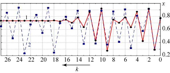
Figure 1: The dependencies of $x$-value of logistic map (15) on the prehisory time $k$. The reference trajectory $\mathbf{x}_{N-k}$ is shown by bold line, two trajectories $\mathbf{x}_{J1-k}$ $\mathbf{x}_{J2-k}$ (whose end points $\mathbf{x}_{J1}$ $\mathbf{x}_{J2}$ are close to $\mathbf{x}_{N}$) are shown by points $\bullet$ (line 1) and dashed line with points $\blacksquare$ (line 2), respectively. The horizontal axis is shown in the opposite direction

Although the coefficients of the matrixes $\mathbf{C}$ and $\mathbf{\tilde{C}}$ are unknown, the validity of both Eq. (10) and Eq. (12) may be verified if there are $N>m$ nearest neighbors $\mathbf{x}_{Ji}$ of the reference vector $\mathbf{x}_{N}$ and corresponding them vectors $\mathbf{y}_{Ji}$ of the response map. Note also, all vectors $\mathbf{x}_{Ji}$ being close to $\mathbf{x}_{N}$ can be used to check Eq. (12), whereas for the examination of Eq. (10) only vectors $\mathbf{x}_{Ji}$ are applicable whose prehistory trajectory satisfies Eq. (5).

Having tested the presence of the generalized synchronization (e.g., with the help of the auxiliary system approach) we can pick out $m$ nearest neighbors $\mathbf{x}_{Ji}$ (${i=1,\dots,m}$) and corresponding to them vectors $\mathbf{y}_{Ji}$ to determine the coefficients of the matrix $\mathbf{C}$ (or $\mathbf{\tilde{C}}$) with the help of Eq. (10) (or Eq. (12)), respectively) in the same way as it has been done in [12]. Afterwards, having determined the coefficients of the matrix $\mathbf{C}$ (or $\mathbf{\tilde{C}}$) we can now find the vectors $\delta\mathbf{z}_{Ji}$, (${i=m+1,\dots,N}$) as

$$\delta\mathbf{z}_{Ji}=\mathbf{C}\delta\mathbf{x}_{Ji}\quad\mbox{or}\quad\delta\mathbf{z}_{Ji}=\mathbf{\tilde{C}}\delta\mathbf{x}_{Ji}$$ (16)

and compare them with the vectors $\delta\mathbf{y}_{Ji}$ of the response system to check Eq. (10) (or Eq. (12). To characterize the degree of closeness of the vectors $\delta\mathbf{y}_{Ji}$ and $\delta\mathbf{z}_{Ji}$ with each other one can compute the normalized differences

$$\Delta_{Ji}=\frac{||\delta\mathbf{y}_{Ji}-\delta\mathbf{z}_{Ji}||}{||\delta\mathbf{y}_{Ji}||}$$ (17)

for each pair of vectors and build their distributions.

So, the strategy of the investigation of the generalized synchronization essence may be the following. Firstly, Eq. (12) must be checked for the set of vectors $\mathbf{x}_{Ji}$ being nearest to the reference one $\mathbf{x}_{N}$, i.e., all points satisfying requirement (14) must be used. If Eq. (12) is valid, it means that in the generalized synchronization regime the states of discrete maps are connected with each other by the functional relation (2). Alternatively, the violation of Eq. (12) indicates that Eq. (2) being the main definition of the generalized synchronization concept accepted hitherto should be reconsidered. In this case the second step consists in the verification of Eq. (10) (and Eq. (4), respectively) with the help of the consideration only vectors $\mathbf{x}_{Ji}$ whose trajectories $\mathbf{x}_{Ji-k}$ satisfy the requirement (5), with the rest of the vectors $\mathbf{x}_{Ji}$ used previously to check Eq. (12) having to be eliminated from the consideration. Since the length $K$ of the prehistory (or the length of the phase tube) is inversely proportional to the absolute value of the largest conditional Lyapunov exponent $\lambda_{1}^{r}<0$, it may be estimated as $K\sim 1/{|\lambda_{1}^{r}|}$.

In this Letter the generalized synchronization in the discrete maps is studied for two sample systems: two unidirectionally coupled logistic maps and two mutually coupled Hénon maps. As we will see below, the concept of the generalized synchronization for the discrete maps needs refining in the same way as it has been done for the flow systems, since, in the general case, for the state vectors of the interacting chaotic maps the prehistory must be taken into account. As a consequence, the division of generalized synchronization into weak and strong ones must also be reconsidered. At the same time, fortunately, this modification of the generalized synchronization concept does not discard the majority of the obtained hitherto results concerning generalized synchronization.

3 Logistic maps

As the first example we consider two unidirectionally coupled logistic maps:

$$\begin{array}[]{l}x_{n+1}=f(x_{n},a_{x}),\\ y_{n+1}=f(y_{n},a_{y})+\sigma(f(x_{n},a_{x})-f(y_{n},a_{y})),\end{array}$$ (18)

where $f(x,a)=ax(1-x)$, $a_{x}=3.75$, $a_{y}=3.79$ are the control parameter values of the drive and response systems, respectively, $\sigma$ characterizes the coupling strength between systems [9]. Despite of the fact that logistic map is the one-dimensional discrete system, it is the etalon object of nonlinear dynamics demonstrating the wide spectrum of interesting effects, and, therefore, it is typically used to study different phenomena including chaotic synchronization. Additionally, the logistic map belongs to the non-invertible discrete systems, for which the existence of the functional relation is not proven. Due to the one-dimensional character of interacting systems (18) the vectors in discussion given above should be replaced by scalars, whereas all theoretical and analytical findings remain correct.

To detect the generalized synchronization regime we have computed conditional Lyapunov exponent for system (18) with further refinement of the threshold values with the help of the auxiliary system method [11]. In Fig. 2 the dependence of the conditional Lyapunov exponent on the coupling parameter $\sigma$ is shown. It is clearly seen that conditional Lyapunov exponent is negative for $\sigma\in[0.12;0.18]$ and $\sigma\geq 0.265$ that is the evidence of the presence of the generalized synchronization regime in these regions. At that, the generalized synchronization is close to the complete (strong) one if the coupling parameter is a great enough, i.e. $\sigma\geq 0.265$, whereas for $\sigma\in[0.12;0.18]$ the detected regime corresponds to the so-called weak synchronization. It is clear that as in the case of the flow systems in the strong generalized synchronization there is no need to take prehistory into account because the drive and response system states are related with each other by the simple functional relation $y_{n}\approx x_{n}$ [9]. At the same time, the case of weak synchronization (when $\sigma\in[0.12;0.18]$) demands the additional investigation.

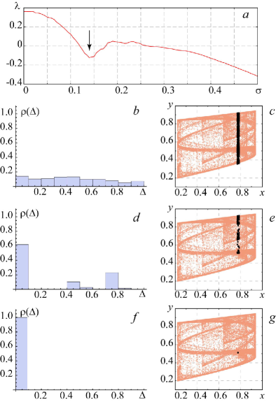
Figure 2: Dependence of the conditional Lyapunov exponent on the coupling parameter $\sigma$ (a); histograms of the normalized differences $\Delta_{Ji}$ built by $N=1000$ neighbor points (b,d,f) and $(x,y)$-planes (c,e,g) for two unidirectionally coupled logistic maps (18) being in the generalized synchronization regime ($\sigma=0.14$, marked by arrow in this figure (a)) for the different lengths of the prehistory: $K=0$ (the number of iteration used to achieve reasonable statistics is $L\sim 3.3\times 10^{4}$) (b,c), $K=10$ ($L\sim 5.5\times 10^{6}$) (d,e), $K=28$ ($L\sim 6.06\times 10^{10}$) (f,g). In Fig. 2,c,e,g the points of the interacting systems satisfying requirement (5) are also shown

Without the loss of generality we fix the coupling parameter to be ${\sigma=0.14}$ that corresponds to the minimum negative value of the conditional Lyapunov exponent (marked by arrow in Fig. 2,a). Having assumed the value of the accuracy in Eq. (5) $\varepsilon=0.01$ we have analyzed the influence of the length $K$ of the prehistory interval on the points $\delta y_{Ji}$ and normalized differences (17), with the reference point $x_{N}$ being selected randomly. Obviously, when Eq. (10) (or Eq. (12)) is satisfied the distribution of normalized differences $\Delta_{Ji}$ should be the $\delta$-function.

Fig. 2,b,d,f illustrates the histograms of the normalized differences $\Delta_{Ji}$ with the increase of the length $K$ of the prehistory. Histograms have been built by $N=1000$ neighbor points being closed to each other during all prehistory interval with the length $K$. To achieve such reasonable statistics for a given value of accuracy $\varepsilon$ we have done $L$ iterations the quantitative values of which are indicated in the caption to Fig. 2. In Fig. 2,c,e,g the $(x,y)$-planes characterizing the drive and response system states for the selected values of the control parameters are also shown. In each figure the points $(x_{Ji},y_{Ji})$ of the interacting systems for which requirement (5) is fulfilled are also indicated. Fig. 2,b,c corresponds to the case when the prehistory is not taken into account at all, i.e., $K=0$. This consideration (without the prehistory) corresponds to the traditional concept of the generalized synchronization generally accepted hitherto. It is clearly seen that in this case the normalized differences $\Delta_{Ji}$ are distributed uniformly over the range $[0;1]$ (Fig. 2,b), at that all points in the phase space of the response system are also allocated randomly in the wide range of the $y$-value variation (Fig. 2,c). So, we have to conclude that Eq. (12) fails and, as a consequence, the traditional viewpoint on the generalized synchronization regime in the discrete systems needs refining.

When the length of the prehistory increases, e.g., for $K=10$ (Fig. 2,d,e), the separate peaks in the normalized difference distribution are revealed (they are exist due to the inhomogeneity of the chaotic attractor), although the points $y_{Ji}$ in the phase space of the response system remain distributed in the wide range of the $y$-value as before. Finally, Fig. 2,f,g illustrates the analogous distributions for the optimal length of the prehistory interval ($K=28$). In this case the distribution of the normalized differences $\Delta_{Ji}$ is the $\delta$-function (Fig. 2,f), and all considered system states $(x_{Ji},y_{Ji})$ satisfying requirement (5) are compressed into small neighbourhood of the reference point $(x_{N},y_{N})$ (Fig. 2,g).

So, having implemented the strategy developed above we can conclude that the relationship between states of the interacting logistic maps involves the prehistory of the drive system evolution in the same way as it has been revealed recently for the systems with continuous time [12].

4 Hénon maps

As the second example we consider two mutually coupled Hénon maps. The mutual type of coupling between interacting systems has been selected for the purpose of universality, i.e. the mutual coupling is so typical as the unidirectional one but analysis of the generalized synchronization regime is performed predominantly in the unidirectionally coupled dynamical systems. There are also attempts to extend the concept of such phenomenon to the systems with a bidirectional type. For example, in our previous works [16, 17] we have shown that the generalized synchronization regime in mutually coupled chaotic systems could be detected by the moment of transition of the second positive Lyapunov exponent in the field of the negative values.

The system under study is given by:

$$\begin{array}[]{l}x^{1}_{n+1}=f(x^{1}_{n},x^{2}_{n},a_{x})+\sigma(f(y^{1}_{n},y^{2}_{n},a_{y})-f(x^{1}_{n},x^{2}_{n},a_{x})),\\ x^{2}_{n+1}=bx^{1}_{n},\\ y^{1}_{n+1}=f(y^{1}_{n},y^{2}_{n},a_{y})+\sigma(f(x^{1}_{n},x^{2}_{n},a_{x})-f(y^{1}_{n},y^{2}_{n},a_{y})),\\ y^{2}_{n+1}=by^{1}_{n},\\ \end{array}$$ (19)

where $\mathbf{x}=(x^{1},x^{2})$ [$\mathbf{y}=(y^{1},y^{2})$] are the vector-states of the first [second] system, $f(x_{1},x_{2},a)=ax_{1}(1-x_{1})+x_{2}$ is the nonlinear function, $a_{x}=3.16779$, $a_{y}=2.9$, $b=0.3$ are control parameters, $\sigma$ is the coupling parameter [18, 19]. For the selected values of the control parameters generalized synchronization determined by the moment of the transition of the second positive Lyapunov exponent in the field of the negative values [16, 20] arises at $\sigma\approx 0.035$.

Now, we fix the coupling parameter to be $\sigma=0.2$ and apply the strategy of the investigation of the generalized synchronization essence (see above) to the system under study. For the chosen value of the coupling parameter the weak generalized synchronization is observed in system (19). As in the case of the logistic maps we characterize the degree of closeness of the vectors $\mathbf{y}_{Ji}$ and $\mathbf{z}_{Ji}$ by histograms of the normalized differences (17) built by $N=100$ neighbor points. The quantitative values of iterations $L$ used to achieve such statistics are also shown in the caption of Fig. 3. At the same time, contrary to the case of the logistic maps considered above, the system under study allows to visualize the behavior of the vectors $\mathbf{y}_{Ji}$ and $\mathbf{z}_{Ji}$ in a plane. Therefore, in Fig. 3 along with the distributions of the normalized differences $\Delta_{Ji}$ (Fig. 3,a,c) the vectors $\mathbf{y}_{Ji}$ ($\circ$) and $\mathbf{z}_{Ji}$ ($\blacksquare$) (Fig. 3,b,d) of the second Hénon map (19) are shown. Fig. 3,a,b corresponds to the case when all the nearest vectors $\mathbf{x}_{Ji}$ satisfying requirement (14) with $\varepsilon=0.01$ are used (i.e., the length of the prehistory interval is $K=0$ and Eq. (12) is examined), whereas Fig. 3,b,c refers to the case when the prehistory of the length $K=40$ is taken into account (in this case the requirement (5) with $\varepsilon=0.01$ is fulfilled and Eq. (10) is verified). It is clearly seen that in the first case the normalized differences $\Delta_{Ji}$ are distributed uniformly over the unit interval (as in the case of the logistic maps considered above) and the vectors $\mathbf{z}_{Ji}$ and $\mathbf{y}_{Ji}$ differ from each other sufficiently that testifies the failure of the presence of the functional relation between the interacting system states. But, conversely, for the second case when the prehistory is taken into account the distribution of $\Delta_{Ji}$ is a $\delta$-function and the calculated vectors $\mathbf{z}_{Ji}$ are in the excellent agreement with the vectors $\mathbf{y}_{Ji}$ of the second map that confirms the theoretical predictions and results obtained above for the unidirectionally coupled logistic maps. So, for in the two-dimensional maps coupled mutually the vector states of the interacting chaotic systems are not also related with each other by the continuously differentiable functional relation and, again, the prehistory should be be taken into account.

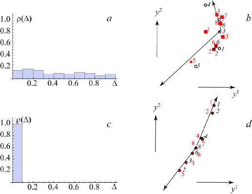
Figure 3: Histograms of the normalized differences $\Delta_{Ji}$ built by $N=100$ neighbor points (a,c) and the vectors $\mathbf{y}_{Ji}$ ($\circ$) and $\mathbf{z}_{Ji}$ ($\blacksquare$) (b,d) of the second Hénnon map (19), $\sigma=0.2$, for the different lengths of the prehistory interval: $K=0$ (the number of iterations used to achieve reasonable statistics is $L\sim 5.9\times 10^{4}$) (a,b), $K=40$ ($L\sim 6.2\times 10^{11}$) (c,d). The numbers $i$ of the vectors $\mathbf{y}_{Ji}$ and $\mathbf{z}_{Ji}$ are shown by the italic and regular fonts, respectively

5 Weak and strong generalized synchronization

In the final part of our Letter we discuss briefly the existing concept of the weak and strong synchronization (see, e.g., [9]) concerning the generalized synchronization regime. As it has been mentioned above, the strong and weak types of the generalized synchronization are typically distinguished, according to the properties of the functional relation between states of the systems. The onset of generalized synchronization is believed to be characterized by an unsmooth map $\mathbf{F}$ that becomes smooth only at sufficiently large coupling strength. The synchronization types characterized by a smooth and an unsmooth map were called a strong and weak synchronization, respectively, with the complete and lag synchronization being a particular case of strong synchronization. This statement [9] was based on the calculation of correlation dimension (and other characteristics) of attractors in the phase space $\mathbb{D}\oplus\mathbb{R}$ (where $\mathbb{D}$ and $\mathbb{R}$ are the phase spaces of the drive and response oscillators, respectively).

Indeed, if one consider the attractor of two coupled logistic maps in the $\mathbb{D}\oplus\mathbb{R}$-space (see Fig. 2,c), the fractal properties of it may be easily revealed. At the same time, the fractality of the relationship $\mathbf{F}$ between states of the interacting systems is caused by the assumption of the existence of the simple function relation (1) between system states and neglecting the prehistory. As it has been discussed above, the states of the interacting systems may be not related with each other by the functional relation and the prehistory must be taken into account. To introduce the prehistory into the consideration in the $\mathbb{D}\oplus\mathbb{R}$-space only vectors $\mathbf{y}_{Ji}$ must be used which satisfy requirement (5) (see Fig. 2,g). As one can see, in this case all considered system states $(x_{Ji},y_{Ji})$ satisfying requirement (5) are compressed into small neighbourhood of the reference point $(x_{N},y_{N})$, all fractal properties disappear and the relation $\mathbf{F}$ between the drive and response system states are smooth. The same conclusion can be drawn not only for the logistic maps (18) but for the general case (3).

Nevertheless, the concept of the weak and strong types of the generalized synchronization may be used in the improved form. This improvement consists in the following. When the state of the second system $\mathbf{y}_{n}$ depends on the prehistory (see Eq. (4)) with the length $K$ this type of the synchronous dynamics should be considered as the weak generalized synchronization. With the growth of the coupling strength the required length $K$ of the prehistory decreases, and, for the certain value of the coupling parameter $\sigma$ the length $K$ becomes equal to zero and the complete synchronization regime is observed in the system. Since for the unidirectionally coupled oscillators the length of the prehistory $K$ depends on the value of the maximum conditional Lyapunov exponent $\lambda_{1}^{r}$, the behavior of the prehistory length agrees well with the finding that the strong generalized synchronization occurs, when the maximum conditional Lyapunov exponent drops below the minimum exponent of the drive system [21]. When the maximum conditional Lyapunov exponent becomes less then the minimum exponent of the drive oscillator, the response system starts to be in some sense stiff enough to follow the external signal, whereas the required prehistory length $K$ is equal to zero. In this case the states of the interacting systems are related with each other by the continuously differentiable functional relation (2) that should be considered as the strong generalized synchronization.

So, the division of the generalized synchronization in discrete maps on the weak and strong ones is certainly justified. At the same time, the difference between them is not determined by the type of the relation $\mathbf{F}$ established between the interacting system states (whether it is smooth or fractal), it is smooth in both cases, at that in the case of strong synchronization the interacting system states are related with each other by the functional relation (2), whereas in for the weak one the prehistory should be taken into account.

6 Conclusions

In conclusion, we have reported that as in the case of the flow systems the concept of generalized synchronization in discrete maps (coupled both unidirectionally and mutually) needs refining, since for the state vectors of the interacting chaotic systems, in general, the prehistory should be taken into account. We have proposed the modification of the phase tube approach applicable to the discrete maps and analyzed the essence of the generalized synchronization by means of such technique. Obtained results show that the division of the generalized synchronization into the weak and the strong ones also needs refinement, i.e. in the strong synchronization interacting system states are related with each other by the continuously differentiable functional relation whereas in the weak one the prehistory should be taken into account for the analysis of the generalized synchronization regime. At that, both in the case of the strong and weak synchronization relation established between the interacting system states is smooth, and the so called “fractality” disappears when the appropriate consideration of the prehistory is made.

At the same time, the found refinement of the generalized synchronization in discrete maps does not discard the majority of the obtained hitherto results concerning its investigation. In particular, the method of Lyapunov exponent computation and auxiliary system approach remains valid as before as well as the revealed mechanisms of the synchronous regime arising [10, 5]. However, this refinement has an important fundamental significance from the point of view of the understanding of the core mechanisms of the considered phenomena and is supposed to give a strong potential for new approaches and applications dealing with the nonlinear systems. Additionally, we expect that the phase tube approach gives a powerful detection and classification tool for the chaotic synchronization phenomenon study.

7 Acknowledgement

We thank the Referees of our manuscript for useful comments and remarks. This work has been supported by Federal special-purpose programme “Scientific and educational personnel of innovation Russia”, Russian Foundation for Basic Research (project 12-02-00221), President’s program (MK-672.2012.2) and “Dynasty” Foundation.

References

- Glass [2001] L. Glass, Synchronization and rhythmic processes in physiology, Nature (London) 410 (2001) 277–284.
- Boccaletti et al. [2002] S. Boccaletti, J. Kurths, G. V. Osipov, D. L. Valladares, C. S. Zhou, The synchronization of chaotic systems, Physics Reports 366 (2002) 1.
- Koronovskii et al. [2009] A. A. Koronovskii, O. I. Moskalenko, A. E. Hramov, On the use of chaotic synchronization for secure communication, Physics-Uspekhi 52 (2009) 1213–1238.
- Rulkov et al. [1995] N. F. Rulkov, M. M. Sushchik, L. S. Tsimring, H. D. I. Abarbanel, Generalized synchronization of chaos in directionally coupled chaotic systems, Phys. Rev. E 51 (1995) 980–994.
- Hramov et al. [2005a] A. E. Hramov, A. A. Koronovskii, O. I. Moskalenko, Generalized synchronization onset, Europhysics Letters 72 (2005a) 901–907.
- Hramov et al. [2005b] A. E. Hramov, A. A. Koronovskii, P. V. Popov, Generalized synchronization in coupled Ginzburg–Landau equations and mechanisms of its arising, Phys. Rev. E 72 (2005b) 037201.
- Filatov et al. [2006] R. A. Filatov, A. E. Hramov, A. A. Koronovskii, Chaotic synchronization in coupled spatially extended beam-plasma systems, Phys. Lett. A 358 (2006) 301–308.
- Dmitriev et al. [2009] B. S. Dmitriev, A. E. Hramov, A. A. Koronovskii, A. V. Starodubov, D. I. Trubetskov, Y. D. Zharkov, First experimental observation of generalized synchronization phenomena in microwave oscillators, Physical Review Letters 102 (2009) 074101.
- Pyragas [1996] K. Pyragas, Weak and strong synchronization of chaos, Phys. Rev. E 54 (1996) R4508–R4511.
- Hramov and Koronovskii [2005] A. E. Hramov, A. A. Koronovskii, Generalized synchronization: a modified system approach, Phys. Rev. E 71 (2005) 067201.
- Abarbanel et al. [1996] H. D. I. Abarbanel, N. F. Rulkov, M. M. Sushchik, Generalized synchronization of chaos: The auxiliary system approach, Phys. Rev. E 53 (1996) 4528–4535.
- Koronovskii et al. [2011] A. A. Koronovskii, O. I. Moskalenko, A. E. Hramov, Nearest neighbors, phase tubes, and generalized synchronization, Phys. Rev. E 84 (2011) 037201.
- Hramov et al. [2006] A. E. Hramov, A. A. Koronovskii, O. I. Moskalenko, Are generalized synchronization and noise-induced synchronization identical types of synchronous behavior of chaotic oscillators?, Phys. Lett. A 354 (2006) 423–427.
- Kocarev and Parlitz [1996] L. Kocarev, U. Parlitz, Generalized synchronization, predictability, and equivalence of unidirectionally coupled dynamical systems, Phys. Rev. Lett. 76 (1996) 1816–1819.
- Koronovskii et al. [2005] A. A. Koronovskii, A. E. Hramov, A. E. Khramova, Synchronous behavior of coupled systems with discrete time, JETP Letters 82 (2005) 160–163.
- Moskalenko et al. [2010] O. I. Moskalenko, A. A. Koronovskii, A. E. Hramov, S. A. Shurygina, Generalized synchronization in mutually coupled dynamical systems, in: Proceedings of 18th IEEE Workshop on Nonlinear Dynamics of Electronic Systems, pp. 70–73.
- Moskalenko et al. [2011] O. I. Moskalenko, A. A. Koronovskii, A. E. Hramov, S. Boccaletti, Generalized synchronization in mutually coupled oscillators and complex networks, Phys. Rev. E (2011).
- Pyragas [1997] K. Pyragas, Conditiuonal Lyapunov exponents from time series, Phys. Rev. E 56 (1997) 5183–5188.
- Pyragas [1998] K. Pyragas, Properties of generalized synchronization of chaos, Nonlinear Analysis: Modelling and Control IMI (1998) 101–129.
- Koronovskii et al. [2011] A. A. Koronovskii, O. I. Moskalenko, V. A. Maksimenko, A. E. Hramov, Appearance of generalized synchronization in mutually coupled beam plasma systems, Technical Physics Letters 37 (2011) 611–614.
- Hunt et al. [1997] B. R. Hunt, E. Ott, J. A. Yorke, Differentiable generalized synchronization of chaos, Phys. Rev. E 55 (1997) 4029–4034.