Two-temperature Langevin dynamics in a parabolic potential

Abstract

We study a planar two-temperature diffusion of a Brownian particle in a parabolic potential. The diffusion process is defined in terms of two Langevin equations with two different effective temperatures in the $X$ and the $Y$ directions. In the stationary regime the system is described by a non-trivial particle position distribution $P(x,y)$, which we determine explicitly. We show that this distribution corresponds to a non-equilibrium stationary state, characterised by the presence of space-dependent particle currents which exhibit a non-zero rotor. Theoretical results are confirmed by the numerical simulations.

Keywords: Two-dimensional diffusion, parabolic potential, non-equilibrium stationary state, rotating flows

1 Introduction

The idea of physical systems characterised by two different temperatures has been proposed a long time ago for the models of spin-glasses and neural networks with partially annealed disorder [1, 2, 3, 4]. In these models, the two temperatures $T_{1}$ and $T_{2}$ are related to two different degrees of freedom, which are evolving at two essentially different time scales. As an example, one may consider a system in which the fast spin variables are connected with the thermal bath kept at the temperature $T_{1}$, while the slow spin-spin coupling parameters are connected with another thermal bath maintained at the temperature $T_{2}$. It can be easily shown that in the stationary (non-equilibrium) state the statistical properties of such systems are described by the usual replica theory of disordered systems with a finite value of the replica parameter $n=T_{1}/T_{2}$ (see also [5]). Unfortunately, generalisation of this idea to the case when dynamics of two types of degrees of freedom is characterised by two comparable (or equal) time scales turned out to be rather problematic: it seems that there is no generic explicit expression for the stationary probability distribution function which would generalise the Gibbs distribution of the equilibrium case $T_{1}=T_{2}$ [6]. However, there is a particular case for which one can find an explicit and a rather non-trivial expression for the stationary distribution function. Namely, this is the case when the two degrees of freedom $x$ and $y$ related to the thermal baths with the temperatures $T_{x}\not=T_{y}$ respectively, experience a potential which is a quadratic function of $x$ and $y$ [6, 7]. During last decade theoretical investigations of such type of systems were mostly concentrated on the studies of nonequilibrium fluctuations and energy transfer [8]. Recently this type of model was studied both theoretically [9] and experimentally [10] from the point of view of the entropy production and memory effects. In this paper, keeping in mind putative experimental realisation of such a type of systems, we are going to discuss the two-temperatures situation reformulated in terms of the two-dimensional diffusion of a Brownian particle in a parabolic potential. The diffusion process is defined in terms of Langevin dynamics with two different effective temperatures in the $X$ and the $Y$ directions. In the stationary state this system is described by a non-trivial distribution function $P(x,y)$, which can be computed explicitly. Unlike for the equilibrium case ($T_{x}=T_{y}$), this non-equilibrium stationary state is characterised by the presence of nontrivial space dependent particle’s flows ${\bf j}(x,y)$. Moreover, these flows exhibit a ”symmetry breaking” rotor, $S(x,y)={\boldsymbol{\nabla}}\times{\bf j}(x,y)$ (directed perpendicular to the $(X,Y)$-plain), the sign (or the direction) of which is determined by the temperature difference $(T_{x}-T_{y})$.

The paper is organised as follows. In Section 2 we define our model and present the explicit solution for the stationary particle’s probability distribution function $P(x,y)$. In Section 3 we compute putative ”observable” quantities of the system, such as the variances of the particle displacements in the $X$ and the $Y$ directions, the rotor $S(x,y)$ of the particle’s flows as well as the average rotation velocity. In Section 4 we report the results of the numerical simulations and compare them with our analytical predictions. Finally, in Section 5 we conclude with a brief recapitulation of our results.

2 The model

We consider stochastic, over-damped Langevin dynamics of a particle moving in a two-dimensional space in a presence of an external potential $U(x,y)$. The particle instantaneous position $\rho(t)$ is defined by projections on the $X$ and the $Y$ axes, $x(t)$ and $y(t)$, respectively. The time evolution of $x(t)$ and $y(t)$ is described by following equations:

$$\frac{d}{dt}x(t) = -\frac{\partial}{\partial x}U(x,y)\;+\;\xi_{x}(t)$$

$$\frac{d}{dt}y(t) = -\frac{\partial}{\partial y}U(x,y)\;+\;\xi_{y}(t)$$

Here $\xi_{x,y}(t)$ is anisotropic stochastic noise, with zero mean and correlation function

$$\left<\xi_{\alpha}(t)\xi_{\beta}(t^{\prime})\right>\;=\;2\,T_{\alpha}\,\delta_{\alpha,\beta}\,\delta(t-t^{\prime})\;,\;\;\;\;\;\;\;(\alpha,\beta\;=x,\;y)$$ (2)

where $T_{x}$ and $T_{y}$ are two different ”temperatures” and $U(x,y)$ has the following parabolic form :

$$U(x,y)\;=\;\frac{1}{2}\,x^{2}\;+\;\frac{1}{2}\,y^{2}\;+\;u\,xy,$$ (3)

The shape of the potential is controlled by the parameter $u$. To keep the particle localised near the origin, we have to impose the constraint $|u|<1$. This follows from the requirement that both eigenvalues of the potential, $\lambda_{1,2}=1\pm u$, must be positive; in the case $|u|>1$, there is a direction in the plane $(x,y)$ at which the potential $U(x,y)$ has a negative curvature which allows the particle to escape to infinity.

In the stationary regime, the probability distribution function $P(x,y)$ of the particle position obeys the stationary Fokker-Planck equation :

$$\frac{\partial}{\partial x}\Bigl{[}T_{x}\frac{\partial P(x,y)}{\partial x}\;+\;P(x,y)\frac{\partial U(x,y)}{\partial x}\Bigr{]}\;+\;\frac{\partial}{\partial y}\Bigl{[}T_{y}\frac{\partial P(x,y)}{\partial y}\;+\;P(x,y)\frac{\partial U(x,y)}{\partial y}\Bigr{]}\;=\;0$$ (4)

In the trivial isotropic case, $T_{x}=T_{y}=T$, the solution of the above equation is simply the equilibrium Gibbs distribution $P_{iso}(x,y)\propto\exp\{-\frac{1}{T}\,U(x,y)\}$.

One can easily show that in the generic anisotropic case with arbitrary $T_{x}$ and $T_{y}$, the solution of the stationary equation (4) reads:

$$P(x,y)\;=\;Z^{-1}\exp\Bigl{\{}-\frac{1}{2}\gamma_{1}\,x^{2}-\frac{1}{2}\gamma_{2}\,y^{2}-u\gamma_{3}\,xy\Bigr{\}}$$ (5)

where the following shortenings have been used

$$\gamma_{1} = \frac{T_{x}+\frac{1}{2}u^{2}(T_{x}-T_{y})}{T_{x}T_{y}\bigl{(}1+u^{2}\Delta^{2}\bigr{)}},$$ (6)

$$\gamma_{2} = \frac{T_{y}+\frac{1}{2}u^{2}(T_{y}-T_{x})}{T_{x}T_{y}\bigl{(}1+u^{2}\Delta^{2}\bigr{)}},$$ (7)

$$\gamma_{3} = \frac{T_{x}+T_{y}}{2T_{x}T_{y}(1+u^{2}\Delta^{2})},$$ (8)

and

$$\Delta\;=\;\frac{(T_{y}-T_{x})}{2\sqrt{T_{y}T_{x}}}.$$ (9)

Further on, $Z$ is the normalisation constant (the ”partition function”), defined as

$$Z = \int\int_{-\infty}^{+\infty}dx\,dy\,\exp\Bigl{\{}-\frac{1}{2}\gamma_{1}\,x^{2}-\frac{1}{2}\gamma_{2}\,y^{2}-u\gamma_{3}\,xy\Bigr{\}}$$ (10)

$$= 2\pi\,\sqrt{\frac{T_{x}T_{y}\bigl{(}1+u^{2}\Delta^{2}\bigr{)}}{1-u^{2}}}.$$

One immediately observes that $Z$ exists, so that the system has the stationary solution, only for $|u|<1$.

3 The observable quantities

3.1 Variances of particle positions

Using the above probability distribution function we can straightforwardly calculate the variances of the particles position with respect to the $X$ and the $Y$ axes:

$$\langle x^{2}\rangle = \frac{T_{x}+\frac{1}{2}u^{2}(T_{y}-T_{x})}{1-u^{2}},$$ (11)

$$\langle y^{2}\rangle = \frac{T_{y}+\frac{1}{2}u^{2}(T_{x}-T_{y})}{1-u^{2}}.$$ (12)

The characteristic quantity, which can serve as the measure of anisotropy in the system under study, is defined as the ratio of these two quantities :

$$g\bigl{(}T_{y}/T_{x};\;u\bigr{)}\;\equiv\;\frac{\langle x^{2}\rangle}{\langle y^{2}\rangle}\;=\;\frac{2+u^{2}\bigl{(}T_{y}/T_{x}-1\bigr{)}}{2T_{y}/T_{x}+u^{2}\bigl{(}1-T_{y}/T_{x}\bigr{)}}$$ (13)

In the trivial decoupled case, $u=0$, we find $g\bigl{(}T_{y}/T_{x};\;0\bigr{)}=T_{x}/T_{y}$, while in the isotropic case, $T_{x}=T_{y}$ we have $g\bigl{(}1;\;u\bigr{)}=1$ for all values of the coupling parameter $u$. Note next that in the strongly anisotropic case, e.g., when $T_{y}/T_{x}\gg 1$, one has

$$\langle x^{2}\rangle \simeq \frac{u^{2}}{2(1-u^{2})}T_{y}$$ (14)

$$\langle y^{2}\rangle \simeq \frac{2-u^{2}}{2(1-u^{2})}T_{y}$$ (15)

$$g \simeq \frac{u^{2}}{2-u^{2}}$$ (16)

In other words, in the strongly anisotropic case the values of both $\langle x^{2}\rangle$ and $\langle y^{2}\rangle$ are defined by the largest $T$, while the value of the ratio $g=\langle x^{2}\rangle/\langle y^{2}\rangle$ becomes a $T$-independent constant.

3.2 Mean rotation velocity

In the stationary case the current ${\bf j}=(j_{x},j_{y})$ is defined as follows:

$$j_{x} = T_{x}\frac{\partial P(x,y)}{\partial x}+P(x,y)\frac{\partial U(x,y)}{\partial x}$$ (17)

$$j_{y} = T_{y}\frac{\partial P(x,y)}{\partial y}+P(x,y)\frac{\partial U(x,y)}{\partial y}$$ (18)

Using eqs.(3)-(5) we obtain :

$$j_{x} = \Bigl{[}(1-T_{x}\gamma_{1})x+u(1-T_{x}\gamma_{3})y\Bigr{]}\,P(x,y)$$ (19)

$$j_{y} = \Bigl{[}(1-T_{y}\gamma_{2})y+u(1-T_{y}\gamma_{3})x\Bigr{]}\,P(x,y)$$ (20)

Note that in the isotropic case, $T_{x}=T_{y}=T$, we have $\gamma_{1}=\gamma_{2}=\gamma_{3}=1/T$, so that ${\bf j}\equiv 0$. In the anisotropic case $T_{x}\not=T_{y}$ the above non-trivial pattern of currents can be characterised in terms of the rotor:

$$S(x,y)\;\equiv\;{\boldsymbol{\nabla}}\times{\bf j}(x,y)\;=\;\frac{\partial}{\partial x}\,j_{y}-\frac{\partial}{\partial y}\,j_{x}$$ (21)

In general, the rotor $S(x,y)$ is a rather complicated function of two variables $x$ and $y$, but it is remarkable that the function $S(x,y)$ has a non-zero (and very simple) value at the origin at $x=y=0$:

$$S(0)\;=\;u\,\bigl{(}T_{x}-T_{y}\bigr{)}\gamma_{3}\,Z^{-1}\;=\;\frac{u}{4\pi}\;\frac{T_{x}^{2}-T_{y}^{2}}{T_{x}^{2}T_{y}^{2}}\,\sqrt{\frac{T_{x}T_{y}(1-u^{2})}{(1+u^{2}\Delta^{2})}}$$ (22)

Note that this quantity changes sign from minus (”left rotation”) at $T_{y}>T_{x}$, to plus (”right rotation”) at $T_{y}<T_{x}$.

Due to the presence of a non-zero particle’s current rotor, one finds that the mean particle’s rotation velocity is also non-zero. Indeed, for a given value of the particle’s linear velocity ${\bf v}$ located in the point ${\bf r}$ on the two-dimensional plane, its angular velocity is

$$\omega(t)\;=\;\frac{1}{r^{2}}\,\bigl{(}{\bf v}\times{\bf r}\bigr{)}$$ (23)

where $\bigl{(}{\bf v}\times{\bf r}\bigr{)}$ is the vector product directed along the $z$-axis. Thus, the mean rotation velocity $\langle\omega\rangle$ in the limit of an infinite observation time can be defined as follows:

$$\langle\omega\rangle\;=\;\lim_{\tau\to\infty}\,\frac{1}{\tau}\int_{0}^{\tau}\,dt\;\omega(t)$$ (24)

Changing averaging over time by averaging over ensemble (which will be justified in what follows by numerical simulations) we get:

$$\langle\omega\rangle\;=\;\int d^{2}{\bf r}\;\frac{1}{r^{2}}\,\bigl{(}{\bf j}\times{\bf r}\bigr{)}\;=\;\int_{0}^{2\pi}d\phi\int_{0}^{\infty}dr\;\bigl{(}j_{x}\sin\phi-j_{y}\cos\phi\bigr{)}$$ (25)

Here the average current ${\bf j}$ is defined in eqs.(19)-(20). According to eq.(5), the probability distribution function $P(r,\phi)$ can be represented as follows

$$P(r,\phi)\;=\;Z^{-1}\,\exp\bigl{\{}-\frac{1}{2}\,r^{2}\,\Psi(\phi)\bigr{\}}$$ (26)

where

$$\Psi(\phi)\;=\;\gamma_{1}\cos^{2}(\phi)\;+\;\gamma_{2}\sin^{2}(\phi)\;+\;u\,\gamma_{3}\,\sin(2\phi)$$ (27)

Substituting the explicit expressions for the components $j_{x}$ and $j_{y}$ of the current, eqs.(19)-(20), and using eqs.(6)-(9), we get

$$\bigl{(}j_{x}\sin\phi-j_{y}\cos\phi\bigr{)}\;=\;\frac{u\bigl{(}T_{y}-T_{x}\bigr{)}}{2\;Z}\;r\;\Psi(\phi)\;\exp\bigl{\{}-\frac{1}{2}\,r^{2}\,\Psi(\phi)\bigr{\}}$$ (28)

Substituting eq.(28) into eq.(25) and performing simple integrations we obtain

$$\langle\omega\rangle\;=\;u\,\Delta\,\sqrt{\frac{1-u^{2}}{1+u^{2}\Delta^{2}}}$$ (29)

where the parameter $\Delta$ is defined in eq.(9).

One can easily prove that the maximal value of the mean angular velocity is $\langle\omega\rangle_{max}=1$, and it is achieved either in the limits $\Delta\to-\infty$ (which corresponds to $T_{y}\to 0$ for finite $T_{x}$) or in the limit $\Delta\to+\infty$ (which corresponds to $T_{x}\to 0$ for a finite $T_{y}$), and the value of the coupling parameter $u=1/\sqrt{\Delta}\;\to\;0$.

4 Numerical simulations: Brownian dynamics

To verify our analytical predictions and the underlying assumption that the time-average can be replaced by the ensemble average, we perform numerical simulations of appropriately discretised Langevin equations eqs.(LABEL:1). Substituting the potential $U(x,y)=\frac{1}{2}x^{2}+\frac{1}{2}y^{2}+uxy$ into eqs.(LABEL:1) we first write these equations explicitly:

$$\begin{array}[]{l}\dot{x}(t)=-x-uy+\xi_{x}(t)\\ \dot{y}(t)=-y-ux+\xi_{y}(t)\;,\end{array}$$ (30)

where the variances of the thermal noise components are defined by $\left<\xi_{x}^{2}\right>=2T_{x}$, $\left<\xi_{y}^{2}\right>=2T_{y}$ and $\left<\xi_{x}\xi_{y}\right>=0$.

Discretising Eq. (30) with a time step $\Delta t$, we have :

$$\begin{array}[]{l}x(t+\Delta t)=x(t)-\Delta t(x+uy)+g_{x}(t)\sqrt{2T_{x}\Delta t}\\ y(t+\Delta t)=y(t)-\Delta t(y+ux)+g_{y}(t)\sqrt{2T_{y}\Delta t}\;,\end{array}$$ (31)

where $g_{x}(t)$ and $g_{y}(t)$ are delta-correlated random numbers with Gaussian distribution of unit half-width, $\Delta t\ll 1$, $\sqrt{2T_{x,y}\Delta t}\ll 1$, which are the conditions of a smooth motion. In that case for a free motion of a particle ($U(x,y)=0$) which starts at the origin ($(x(0)=0,\;y(0)=0)$), the diffusion coefficients are $D_{\alpha}=T_{\alpha}$, $\alpha=x,y$ and the variances of the displacement are given by $\left<x^{2}(t)\right>=2T_{x}t$ and $\left<y^{2}(t)\right>=2T_{y}t$. In the case of the symmetric potential ($u=0$), one has in the stationary regime $\left<x^{2}\right>=T_{x}$ and $\left<y^{2}\right>=T_{y}$, independently of $t$. For asymmetric potential $u\neq 0$, we will compute the mean angular velocity $\left<\omega\right>$ given in eq.(24) and the measure of anisotropy $g(T_{y}/T_{x},u)=\left<x^{2}\right>/\left<y^{2}\right>$ that is described by eq.(13).

The numerical simulation has been done for the time step $\Delta t=0.001$. The averaging has been performed over the total time period $\tau=10^{6}$ time units, the numerical inaccuracy has been evaluated by splitting the whole time interval into $10$ sub-intervals. In Fig. 1(a),(b) we plot numerical results for the ratio of variances $\left<x^{2}\right>/\left<y^{2}\right>$ and for the mean angular velocity $\left<\omega\right>$, calculated as the time-average of $\omega(t)$, as functions of $u$ for $T_{x}=1$, $T_{y}=1,2,4,6,8,10$. For comparison we also show our analytical predictions in eq.(13) and eq.(24), respectively, and find a perfect agreement. This justifies the replacement of the time-average by the ensemble average in our analytical calculations.

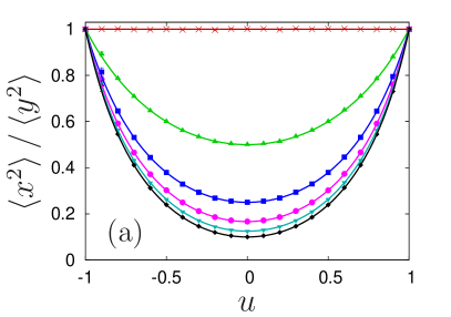
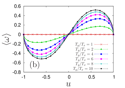
Figure 1: (a) The ratio $\left<x^{2}\right>/\left<y^{2}\right>$ of variances of particle’s displacements along the $X$ and the $Y$-axes vs the parameter $u$. (Symbols and the color-code is as in (b) ); (b) the mean angular velocity $\left<\omega\right>$ as a function of $u$ for different $T_{y}/T_{x}=1,2,4,6,8,10$. Solid lines are our predictions in eqs.(13) and (24).

Further on, in Fig. 2(a),(b) we plot the same quantities as functions of $T_{y}/T_{x}$ (with $T_{x}=1$) for $u=0,0.2,0.4,0.6,0.8,0.9$. We again observe a very good agreement between our numerical and analytical results.

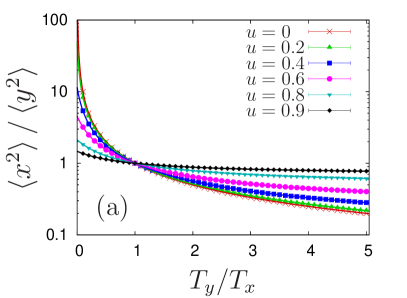
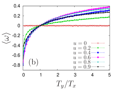
Figure 2: (a) The $\left<x^{2}\right>/\left<y^{2}\right>$ and (b) the mean angular velocity $\left<\omega\right>$ as functions of $T_{y}/T_{x}$ for different values of $u=0,0.2,0.4,0.6,0.8,0.9$. Solid lines define our theoretical predictions in eqs.(13) and (24), and the symbols denote the results of numerical simulations.

5 Conclusions

In the present work we studied a simple stochastic ”toy model” with only two degrees of freedom which are connected to two thermostats maintained at two different temperatures $T_{x}$ and $T_{y}$, respectively. The model describes diffusion of a particle on a two-dimensional plane in a presence of a parabolic potential such that the stochastic noises in the $X$ and the $Y$ directions have different strength ($T_{x}$ and $T_{y}$, respectively). We determine the stationary state probability distribution function for the position of the particle. Despite its relatively simple structure, it turns out to be rather non-trivial, revealing interesting qualitative physical phenomena. In particular, in the stationary state one finds a rather sophisticated pattern of particles’ density currents (which would be identically equal to zero in the equilibrium case) characterised by the non-zero rotor. Moreover, due to the presence of this flux rotor one observes the phenomenon which could be interpreted as a ”spontaneous symmetry breaking”, namely one finds non-zero value for the average particle’s rotation (around the origin) velocity. This value is proportional to $(T_{y}-T_{x})$, eq.(29), being positive (left rotation) for $T_{x}<T_{y}$ and negative (right rotation) for $T_{x}>T_{y}$.

It should be stressed, however, that except for recently proposed two-temperature electric analog system [10], for the moment the considered model has no experimental realization. Thus, the aim of the present work is somewhat provocative: we would like argue that the systems of such type are sufficiently interesting to stimulate investigations for their ”hardware” implementations. We also believe that modifications of our toy model towards a system that could be realised in practice and at the same time would not loose its interesting behavior (rotation), is possible.

6 References

References

- [1] R.W.Penney, T.Coolen and D.Sherrington, J.Phys. A26, 3681 (1993).
- [2] V.S.Dotsenko, S.Franz and M.Mezard, J.Phys. A27, 2351 (1994).
- [3] D.E.Feldman and V.S.Dotsenko, J.Phys. A: Math.Gen., 27, 4401 (1994).
- [4] V.S.Dotsenko, ”Physics of Spin Glasses and Related Problems” in ”The First Landau Institute Summer School, 1993” (Edited by V.Mineev), Gordon and Breach 1995.
- [5] V.S.Dotsenko, ”Introduction to the Theory of Spin Glasses and Neural Networks”, World Scientific 1994.
- [6] V.S.Dotsenko, Lectures on statistical physics of disordered systems for the Landau Institute graduate students, 1995 (unpublished).
- [7] R.Exartier and L.Peliti, Physics Letters A, 261, 94 (1999).
- [8] T.Bodineau and B.Derrida, Phys.Rev.Lett. 92, 180601 (2004); P.Visco, J.Stat.Mech. P06006 (2006); A.Gomez-Martin and J.M.Sancho, Phys.Rev. E 73, 045101 (2005)
- [9] A.Crisanti, A.Puglisi and D.Villamaina, Phys. Rev. E, 85, 061127 (2012); A.Puglisi and D.Villamaina Europhys.Lett. 88, 30004 (2009); D.Villamaina, A.Baldassarri, A.Puglisi and A.Vulpiani J.Stat.Mech. P07024 (2009)
- [10] S.Ciliberto, A.Imparato, A.Naert and M.Tanase, On the heat flux and entropy produced by thermal fluctuations, arXiv:1301.4311 (2013)