Type-II intermittency characteristics in the presence of noise

Abstract

We consider a type of intermittent behavior that occurs as the result of the interplay between dynamical mechanisms giving rise to type-II intermittency and random dynamics. We analytically deduce the law for the distribution of the laminar phases, which has never been obtained hitherto. The already known dependence of the mean length of the laminar phases on the criticality parameter [PRE 68 (2003) 036203] follows as a corollary of the carried out research. We also prove that this dependence obtained earlier under the assumption of the fixed form of the reinjection probability does not depend on the relaminarization properties, and, correspondingly, the obtained expression of the mean length of the laminar phases on the criticality parameter remains correct for different types of the reinjection probability.

1 Introduction

Intermittency is known to be an ubiquitous phenomenon, with its arousal and main statistical properties having been studied and characterized already since long time ago. The different types of intermittency have been classified as types I–III Dubois:1983_IntermittencyIII , on–off intermittency Platt:1993_intermittency ; Heagy:1994_intermittency ; Hramov:2005_IGS_EuroPhysicsLetters , eyelet intermittency Pikovsky:1997_EyeletIntermitt ; Boccaletti:2002_LaserPSTransition_PRL and ring intermittency Hramov:RingIntermittency_PRL_2006 ; Hramov:2007_2TypesPSDestruction . From the other side, increasing interest has been put recently in the study of the constructive role of noise and fluctuations in nonlinear systems. In particular, it was discovered that random fluctuations can actually induce some degree of order in a large variety of nonlinear systems Pikovsky:1997_CoherenceResonance ; Mangioni:1997_Noise ; Hramov:2006_PLA_NIS_GS , and such phenomena were widely observed in relevant physical circumstances Boccaletti:2002_LaserPSTransition_PRL ; Zhou:PRE2003 .

There are no doubts that different types of intermittent behavior may take place in the presence of noise and fluctuations in a wide spectrum of systems, including cases of practical interest for applications in physical, radio engineering and other applied sciences. It is plausible that such an interaction would originate new types of dynamics. Therefore, the intermittent behavior in the presence of noise has been studied by means of Fokker-Plank equation Hirsch:1982_Intermittency and adopting renormalization group analysis Hirsch:1982_IntermittencyPLA , but the characteristic relations were obtained only in the subcritical region, where the intermittent behavior is observed both in the presence of noise and without noise. Recently Kye:2000_TypeIAndNoise ; Cho:2002_TypeINoseExpeiment ; Hramov:2007_TypeIAndNoise , the theoretical and experimental consideration of the intermittent behavior in the presence of noise has been considered in the supercritical region (where intermittency does not take place in the absence of noise) for the type-I intermittency.

Obviously, in the presence of noise the other types of intermittent behavior mentioned above may result in the distinct types of dynamics. In this paper we report for the first time the important characteristic (namely, the distribution of the laminar phase lengths) deduced analytically for the type-II intermittency in the presence of noise for the region of the supercritical parameter values, which has never been obtained hitherto. This characteristic is of great importance, since scientists studying the intermittent behavior of the complex systems often can not variate the criticality parameter in the experiments (e.g., in physiological and biological systems), and, therefore, they can deal only with the the distribution of the laminar phase lengths, whereas the dependence of the mean length of the laminar phases on the criticality parameter can not be obtained. The already known dependence of the mean length of the laminar phases on the criticality parameter Kye:2003_TypeIIAndIIINoiseExperiment follows as a corollary of the carried out research. Moreover, we prove that this dependence obtained in Kye:2003_TypeIIAndIIINoiseExperiment under the assumption of the fixed reinjection probability (taken in the forms of delta-function and uniform distribution) does not depend practically on the relaminarization properties, and, correspondingly, the obtained expression of the mean length of the laminar phases on the criticality parameter remains correct for different forms of the reinjection probability. The obtained analytical distribution of the laminar phase length is verified by means of numerical calculations of the model system dynamics.

2 Analytical approach

The standard model that is used to study the type-II intermittency Kye:2003_TypeIIAndIIINoiseExperiment is the one-parameter cubic map

$$x_{n+1}=f(x_{n})=(1+\epsilon)x_{n}+x_{n}^{3},$$ (1)

where $\epsilon$ is a control parameter. Below the critical parameter value (i.e., for $\epsilon<\epsilon_{c}$), the stable fixed point $x_{c}=0$ is observed, while above $\epsilon_{c}$ this fixed point $x_{c}=0$ becomes unstable and the point representing the state of the map (1) moves around it with slowly increasing amplitude. This movement in the vicinity of the fixed point corresponds to the laminar phase, its mean length $T$ being inversely proportional to $(\epsilon-\epsilon_{c})$, i.e.

$$T\sim(\epsilon-\epsilon_{c})^{-1}.$$ (2)

To develop the theory of type-II intermittency in the presence of noise, we consider the same cubic map (1) with the addition of a stochastic term $\xi_{n}$

$$x_{n+1}=f(x_{n})=(1+\epsilon)x_{n}+x_{n}^{3}+\xi_{n},$$ (3)

where $\xi_{n}$ is supposed to be a delta-correlated white noise [${\langle\xi_{n}\rangle=0}$, ${\langle\xi_{n}\xi_{m}\rangle=D\delta(n-m)}$].

The influence of the stochastic term $\xi_{n}$ on the behavior of the system is governed by the value of parameter $D$. For positive values of the control parameter $\epsilon$ ($\epsilon>0$), the point corresponding to the behavior of system (3) moves in the iteration diagram around the unstable fixed point, its motion being perturbed by the stochastic force. As far as the intensity of the noise is not large, the characteristics being close to the classical type-II intermittency are observed.

A different scenario occurs for control parameters $\epsilon$ assuming negative values ($\epsilon=-\varepsilon$, where $\varepsilon=|\epsilon|>0$). In this case, the point corresponding to the behavior of system (3) is localized for a long time in the region ${-\sqrt{\varepsilon}<x<\sqrt{\varepsilon}}$ and its dynamics is also perturbed by the stochastic force. As soon as the system state point arrives at one of the boundaries $x_{b}=\pm\varepsilon^{-1/2}$ due to the influence of noise, a turbulent phase arises, though such kind of events is very rare.

In this case, the behavior of the map (3) differs radically from the dynamics of the system (1), since the turbulent phases are not observed for $\epsilon<0$ if there is no noise. Therefore, such a region of negative values of the $\epsilon$-parameter is the main subject of interest for the type-II intermittency in the presence of noise.

2.1 Probability density

Having supposed that: (i) the value of $\epsilon$ is negative and rather small and (ii) the value of $x$ changes per one iteration insufficiently, we can consider ${(x_{n+1}-x_{n})}$ as the time derivative $\dot{x}$ and undergo from the system with discrete time (3) to the flow system, in the same way as in the case of the classical theory of the intermittency Dubois:1983_IntermittencyIII .

Since the stochastic term is present in (3) we have to examine the stochastic differential equation

$$dX=X(X^{2}-\varepsilon)\,dt+dW$$ (4)

(where $X(t)$ is a stochastic process, $W(t)$ is a one-dimensional Winner process, $\varepsilon=|\epsilon|$) instead of the ordinary differential equation ${dx/dt=x(x^{2}+\epsilon)}$ considered in the classical theory of type II intermittency.

The stochastic differential equation (4) is equivalent to the Fokker-Plank equation

$$\frac{\partial\rho_{X}}{\partial t}=-\frac{\partial}{\partial x}\left(x(x^{2}-\varepsilon)\rho_{X}\right)+\frac{D}{2}\frac{\partial^{2}\rho_{X}}{\partial x^{2}}$$ (5)

for the probability density $\rho_{X}(x,t)$ of the stochastic process $X(t)$. The chosen initial condition is ${\rho_{X}(x,0)=\delta(x-\Delta)}$, where $\delta(\cdot)$ is a delta-function. Such a choice of the initial form of the probability density $\rho_{X}(x,0)$ corresponds to the beginning of the laminar phase, when the point representing the state of the system (3) is in the place with coordinate $x=\Delta$ ($-\varepsilon^{1/2}<\Delta<\varepsilon^{1/2}$) at time $t=0$. In other words, we suppose that the reinjection probability is a $\delta$-function

$$P_{in}(x)=\delta(x-\Delta)$$ (6)

and after the relaminarization process the system is always returned to the state $x=\Delta$. Although the reinjection probability $P_{in}(x)$ is well-known to be important factor and should be taken into account when the statistical properties of the intermittent behavior are studied Kin:1994_NewIntermittencyCharacteristics ; Kim:1998_IntermittencyCharacteristicsPRL , in the considered problem the form of the reinjection probability practically does not influence on the distribution of the laminar phase lengths (and the dependence of the mean laminar phase length on the criticality parameter, respectively), as it will be shown below.

To reduce the number of the control parameters the normalization $z=x/\sqrt{\varepsilon}$, $\tau=t\varepsilon$ may be used, after which Eq. (5) may be rewritten in the form

$$\frac{\partial\rho_{Z}}{\partial\tau}=-\frac{\partial}{\partial z}\left(z(z^{2}-1)\rho_{Z}\right)+\frac{D^{*}}{2}\frac{\partial^{2}\rho_{Z}}{\partial z^{2}},$$ (7)

where $D^{*}=D\varepsilon^{-2}$, $\rho_{Z}(z,\tau)=\rho_{X}(z{\varepsilon}^{1/2},\tau{\varepsilon}^{-1})$.

As the coordinate of the system state stays for a long time in the region $|z|<z_{b}=1$, one can suppose that the probability density may found the form of the metastable distribution decaying slowly for a long period of time. The relaxation process of the probability density to this metastable state is supposed to be very fast in comparison with the time of the metastable distribution decay, therefore, one can neglect the transient ${0\leq t\leq t_{tr}}$. Under the assumptions made above the probability density may be written in the form ${\rho_{Z}(z,\tau)=A(\tau)g(z)}$, ${\forall z\in(-1;1)}$, where $A(\tau)>0$ decreases very slowly as time increases, i.e. $dA/d\tau\approx 0$. The function $g(z)$ should satisfy the conditions

$$g(z)>0~{}~{}\forall z\in(-1;1)\quad\mathrm{and}\quad\displaystyle\int\limits_{-1}^{1}g(z)\,dz<\infty.$$ (8)

As the maximum of the probability density should coincide with the stable fixed point $z_{s}=0$, one has

$$g^{\prime}(z)\left|{}_{z=0}\right.=0.$$ (9)

Under the mentioned assumption, we consider the ordinary differential equation

$$D^{*}g^{\prime\prime}(z)-2\left(z(z^{2}-1)g(z)\right)^{\prime}=0$$ (10)

instead of (7) for the region $z\in(-1;1)$.

This equation is equivalent to

$$D^{*}g^{\prime}(z)-2z(z^{2}-1)g(z)+C_{1}=0,$$ (11)

where $C_{1}$ is constant. To solve this equation we use the integrating factor

$$M(z)=\exp\left(\frac{z^{2}}{D^{*}}\left(1-\frac{z^{2}}{2}\right)\right).$$ (12)

The solution of (11) may be found in the form

$$g(z)=\frac{\displaystyle 2C_{1}\int_{0}^{z}\exp\left(\frac{s^{2}}{D^{*}}\left(1-\frac{s^{2}}{2}\right)\right)\,ds+C_{2}}{\displaystyle D^{*}\exp\left(\frac{z^{2}}{D^{*}}\left(1-\frac{z^{2}}{2}\right)\right)}.$$ (13)

From Eq. (13) one can obtain easily that ${g^{\prime}(0)=2C_{1}/D^{*}}$. Taking into account the condition (9), one comes to the conclusion that $C_{1}\equiv 0$. Note, in this case the obtained function

$$g(z)=\frac{C_{2}}{D^{*}}\exp\left(-\frac{z^{2}}{D^{*}}\left(1-\frac{z^{2}}{2}\right)\right).$$ (14)

also satisfies the conditions (8). Therefore, the probability density $\rho_{Z}(z,\tau)$ in the region $z\in(-1;1)$ is

$$\rho_{Z}(z,\tau)\simeq A(\tau)\exp\left(-\frac{z^{2}}{D^{*}}\left(1-\frac{z^{2}}{2}\right)\right).$$ (15)

When the laminar phase is interrupted, the system escapes from a metastable state. Therefore, we suppose that the decrease of $A(\tau)$ should be determined by the probability distribution taken in the boundary points $z=\pm 1$, i.e., $dA(\tau)/d\tau\sim-\rho_{Z}(\pm 1,\tau)$. This assumption, which is also equivalent to neglecting the time correlation of the orbit, may be rewritten as

$$\frac{dA(\tau)}{d\tau}=-kA(\tau)\exp\left(-\frac{1}{2D^{*}}\right),$$ (16)

where $k$ is a proportionality coefficient. Evidently, the decrease of $A(\tau)$ is described by the exponential law

$$A(\tau)=A(0)\exp(-k\eta\tau),\quad\eta=\exp{(-1/(2D^{*}))}.$$ (17)

Having returned to the initial variables $x$ and $t$ we derive the following expression for the probability density

$$\rho_{X}(x,t)\simeq A(t)\exp\left(-\frac{x^{2}}{D}\left(\varepsilon-\frac{x^{2}}{2}\right)\right),$$ (18)

where

$$A(t)=A(0)\exp\left(-\frac{t}{T}\right),$$ (19)

and

$$T=\frac{1}{k\varepsilon}\exp\left(\frac{\varepsilon^{2}}{2D}\right),$$ (20)

with $A(t)$ being considered as a normalizing factor, i.e.,

$$A(0)\int\limits_{-\sqrt{\varepsilon}}^{\sqrt{\varepsilon}}\exp\left(-\frac{x^{2}}{D}\left(\varepsilon-\frac{x^{2}}{2}\right)\right)\,dx=1.$$ (21)

To confirm the assumptions made above and the obtained equations, we have compared the evolution of the probability density $\rho_{X}(x,t)$ given by (18) with the result of the direct numerical calculation of the Fokker-Plank equation (5) with the values of control parameters $\varepsilon=10^{-2}$, $D=10^{-5}$.

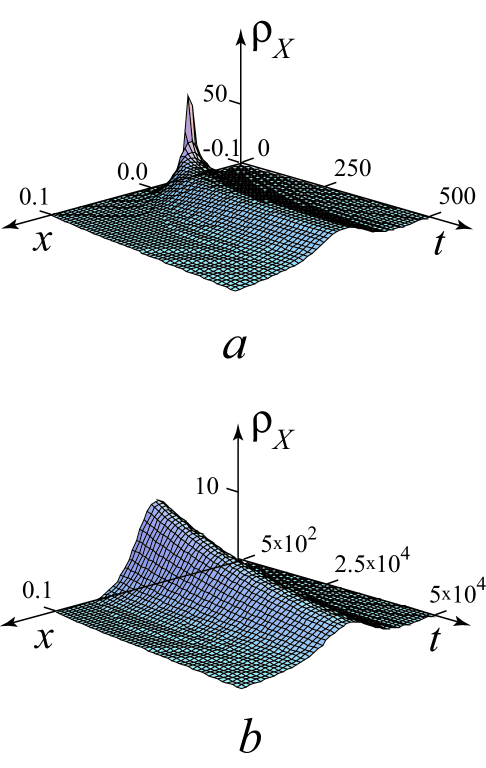
Figure 1: The evolution of the probability density $\rho_{X}(x,t)$ obtained by means of the direct numerical integration of Fokker-Plank equation (5), ${\varepsilon=10^{-2}}$, ${D=10^{-5}}$. (a) The initial fragment of the density evolution involving the transient (${0\leq t<t_{tr}}$, $t_{tr}\approx 3\times 10^{2}$). (b) The long-time evolution of $\rho_{X}(x,t)$, with the transient being omitted, $5\times 10^{2}\leq t\leq 5\times 10^{4}$

The evolution of the probability density $\rho_{X}(x,t)$ obtained by the numerical calculation of (5) is shown in Fig. 1. One can see that after the very short transient ${0\leq t\leq t_{tr}}$ the probability density $\rho_{X}(x,t)$ arrives the state being close to stationary (Fig. 1 a). After that the value of $\rho_{X}(x,t)$ decreases very slowly (according to the exponential law) with time increasing, with the form of the dependence of the probability density on $x$-coordinate being invariable (Fig. 1 b).

Fig. 2 also shows the profiles of the probability density $\rho_{X}(x,t^{*})$ taken in the different moments of time. It is evident, that after a very short transient (curve 1, $t_{1}^{*}=15$), the density $\rho_{X}(x,t)$ practically does not change when time increases.

Two different profiles $\rho_{X}(x,t^{*})$ corresponding to the time moments $t^{*}_{2}=5\times 10^{2}$ and $t^{*}_{3}=3\times 10^{3}$ (curves 2 and 3, respectively) are very close to each other despite of the large time interval $\Delta t={t^{*}_{3}-t^{*}_{2}}$ between them. Moreover, they are in very good agreement with the approximated solution $A(0)g(x)$ described by Eq. (18) and shown in Fig. 2 by means of squares. As time goes on, the amplitude of the probability density decreases according to the exponential law, but very slowly (see Fig. 2, curves 4 and 5, $t^{*}_{4}=10^{4}$ and $t^{*}_{5}=5\times 10^{4}$, respectively), although the probability density form remains the same for all times.

Therefore, taking into account the results of the direct numerical calculations of Fokker-Plank equation (5) and the comparison with the obtained approximated solution (18), we come to the conclusion that our assumptions are correct and can be used for the further analysis.

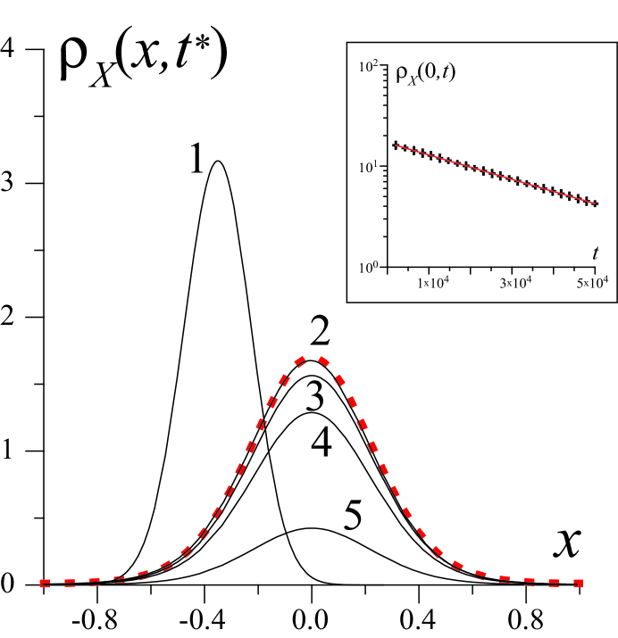
Figure 2: The profiles of the probability density $\rho_{X}(x,t^{*})$ taken in the different moments of time $t^{*}$ obtained from the direct numerical calculation of Fokker-Plank equation (5). In the frame the dependence of the probability density $\rho(0,t)$ in the stationary point $x=0$ on time $t$ ($+$) and its exponential approximation (solid line) are shown in the logarithmic scale

The evolution of the probability density $\rho_{X}(x,t)$ may be considered separately on two time intervals ${0\leq t<t_{tr}}$ and ${t_{tr}\leq t<+\infty}$, respectively. The first time interval corresponds to the transient when the probability density $\rho_{X}(x,t)$ evolves to the form (18) being close to stationary. Only when ${0\leq t<t_{tr}}$ the form of the reinjection probability $P_{in}(x)$ may influence on the evolution of the probability density $\rho_{X}(x,t)$. For $t\geq t_{tr}$ (when the transient is elapsed), the evolution of the probability density is defined completely by Eq. (18) and it does not depend entirely on the reinjection probability $P_{in}(x)$. Since the transient is very short in comparison with the exponential decrease of the probability density $\rho_{X}(x,t)$ we can neglect them and use only the second time interval ${t_{tr}\leq t<+\infty}$ to obtain the statistical characteristics of the type-II intermittent behavior in the presence of noise. It is clear, that in this case the obtained results do not depend on the relaminarization process and the reinjection probability $P_{in}(x)$.

2.2 Distribution of the laminar phase lenghts

Let us discuss now the relationship between the probability density $\rho_{X}(x,t)$ and the distribution $p(t)$ of the laminar phase lenghts $t$. For this purpose we consider the ensemble of systems (4). Let there be $N(t)$ systems which at the moment of time $t$ are in the stage of the laminar phase. Obvioulsy, the states $x$ of these systems should be distributed over interval $(-\sqrt{\varepsilon},\sqrt{\varepsilon})$ according to the probability density $\rho_{X}(x,t)$. After the infinitely small time interval $dt$ several systems stop demonstrating the laminar behavior (the turbulent phase begins in these systems) and, correspondingly, their states $x$ leave the interval $(-\sqrt{\varepsilon},\sqrt{\varepsilon})$, while the states of other $N(t+dt)$ systems demonstrating the laminar dynamics as before are distributed in accordance with the probability density $\rho_{X}(x,t+dt)$). If the total number of the systems in the ensemble under consideration is $N_{0}$, the number of the systems in which the laminar phase is finished during time interval $[t,t+dt)$ is

$$\begin{array}[]{l}\displaystyle N(t)-N(t+dt)=\\ \displaystyle\qquad=N_{0}\int\limits_{-\sqrt{\varepsilon}}^{\sqrt{\varepsilon}}[\rho_{X}(x,t)-\rho_{X}(x,t+dt)]\,dx.\end{array}$$ (22)

Since the number of the systems in the ensemble in which the laminar phase is interrupted at the moment of time falling in the time interval between $t$ and $t+dt$ is connected with the distribution $p(t)$ of the laminar phase lengths $t$ as

$$N(t)-N(t+dt)=N_{0}p(t)\,dt,$$ (23)

one can obtain the relationship

$$p(t)=-\int\limits_{-\sqrt{\varepsilon}}^{\sqrt{\varepsilon}}\frac{\partial\rho_{X}(x,t)}{\partial t}\,dx$$ (24)

between the probability density $\rho_{X}(x,t)$ and the distribution $p(t)$ of the laminar phase lenghts.

Using relations (18), (19) and (21) one can obtain, that the laminar phase distribution is governed by the exponential law

$$p(t)=T^{-1}\exp\left(-{t/T}\right),$$ (25)

where $T$ defined by Eq. (20) is the mean length of the laminar phases. The obtained expression (20) for the mean length $T$ of the laminar phases is consistent with the formal solution derived in the previous considerations Kye:2003_TypeIIAndIIINoiseExperiment ; Pikovsky:1983_IntermittencyWithNoise , that may be considered as an additional evidence of the correctness of our results. Nevertheless, we would like to emphasize that the applicability of the results obtained earlier analytically Kye:2003_TypeIIAndIIINoiseExperiment ; Pikovsky:1983_IntermittencyWithNoise are limited greatly by the assumptions (made to deduce corresponding equation) concerning the character of the reinjection process. Indeed, it is well known that the characteristics of the intermittent behavior even in the case without noise depend not only on the structure of the local Poincare map but on the reinjection probability distribution, with this dependence being sufficient (see e.g., Kin:1994_NewIntermittencyCharacteristics ; Kim:1998_IntermittencyCharacteristicsPRL ). At the same time, the analytical results mentioned above were obtained only under assumptions of uniform and delta-function reinjection probability distribution. Our study allows to extend known relation to all types of the reinjection probability distribution, since based on the consideration carried out above we state that Eqs. (20) and (25) do not depend on the relaminarization process properties and may be used for the arbitrary reinjection probability $P_{in}(x)$.

3 Numerical results

To verify the obtained theoretical predictions, we consider numerically the intermittent behavior of the quadratic map (3) with a stochastic force. The reinjection procedure has been fulfilled as follows: when the value of the $x_{n}$-variable leaves the interval ${-1<x<+1}$, the next its value has been taken as $x_{n+1}=10^{-2}x_{n}$. Since the dependence of the mean laminar phase length on the criticality parameter (20) has already been studied Kye:2003_TypeIIAndIIINoiseExperiment , in our calculations we focus on the consideration of distribution of the laminar phase lengths.

Obviously, if the intensity of noise $D$ is equal to zero the intermittent behavior is observed for $\epsilon>0$, whereas the stable fixed point takes place for $\epsilon<0$. Having added the stochastic force we can expect that the intermittent behavior may be also observed in the area of the negative values of the criticality parameter $\epsilon$.

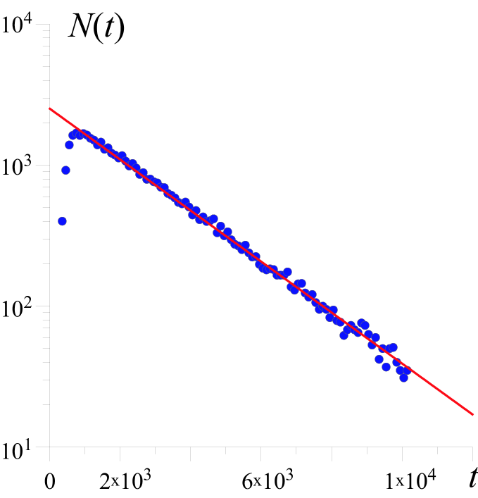
Figure 3: The distribution of the laminar phase lengths for map (3). The criticality parameter value has been selected as $\epsilon=-10^{-3}$, the noise intensity is $D=10^{-6}$. The ordinate axis is presented in the logarithmic scale. The theoretical exponential law (25) is shown by the solid line

The distribution of the laminar phase lengths is in very good accordance with the exponential law (25) predicted by the theory of the type-II intermittency with noise (see Fig. 3). Note the presence of the small region of the short laminar phase lengths in Fig. 3 where the deviation from the prescribed exponential law (25) is observed. This region corresponds to the transient ${0\leq t<t_{tr}}$ when the probability density $\rho_{X}(x,t)$ evolves to the form (18) being close to stationary as it was discussed above. The existence of this transient time interval does not influence practically on the characteristics (20) and (25) of the intermittent behavior in the presence of noise in the full agreement with the conclusions made above. So, the intermittent behavior observed in the quadratic map with the stochastic force agrees well with the theoretical predictions.

4 Conclusion

In conclusion, we have reported a type of intermittency behavior caused by the cooperation between the deterministic mechanisms and random dynamics. The distribution of the laminar phase lengths being one of the important characteristics of the intermittent dynamics has been deduced analytically. Having considered the standard model of type-II intermittency in the presence of noise we can conclude that (i) noise induces new features in the intermittent behavior of a system demonstrating type-II intermittency, with new dynamical properties being observed above the former value of the criticality parameter; (ii) the results of numerical simulations are in excellent agreement with the developed theory; (iii) the relaminarization process properties and the reinjection probability do not seem to play a major role for the statistical characteristic of type-II intermittency, and, the obtained expression of the mean length of the laminar phases on the criticality parameter as well as the dependence of the mean length of the laminar phases on the criticality parameter remain correct for different forms of the reinjection probability.

Though the characterization of the intermittent process has been explicitly derived here for model system, we expect that the very same mechanism can be observed in many other relevant circumstances where the level of natural noise is sufficient, e.g. in the physiological Hramov:2006_Prosachivanie ; Hramov:2006_RAT_ON-OFF ; Hramov:2007_UnivariateDataPRE or physical systems Boccaletti:2002_LaserPSTransition_PRL .

This work has been supported by U.S. Civilian Research & Development Foundation for the Independent States of the Former Soviet Union (CRDF, grant REC–006), Russian Foundation of Basic Research (project 07-02-00044), the Supporting program of leading Russian scientific schools (project NSh–355.2008.2). We thank “Dynasty” Foundation. A.E.H. also acknowledges support from the President Program, Grant No. MD-1884.2007.2.

References

- (1) Dubois M., Rubio M., Bergé P., Phys. Rev. Lett. 51, (1983) 1446.
- (2) Platt N., Spiegel E. A., Tresser C., Phys. Rev. Lett. 70, (1993) 279.
- (3) Heagy J. F., Platt N., Hammel S. M., Phys. Rev. E 49, (1994) 1140.
- (4) Hramov A. E., Koronovskii A. A., Europhysics Lett. 70, (2005) 169.
- (5) Pikovsky A. S., Osipov G. V., Rosenblum M. G., Zaks M., Kurths J., Phys. Rev. Lett. 79, (1997) 47.
- (6) Boccaletti S., Allaria E., Meucci R., Arecchi F. T., Phys. Rev. Lett. 89, (2002) 194101.
- (7) Hramov A. E., Koronovskii A. A., Kurovskaya M. K. Boccaletti S., Phys. Rev. Lett. 97, (2006) 114101.
- (8) Hramov A. E., Koronovskii A. A. Kurovskaya M. K., Phys. Rev. E 75, (2007) 036205.
- (9) Pikovsky A. S. Kurths J., Phys. Rev. Lett. 78, (1997) 775.
- (10) Mangioni S., Deza R., Wio H., Toral R., Phys. Rev. Lett. 79, (1997) 2389.
- (11) Hramov A. E., Koronovskii A. A., Moskalenko O. I., Phys. Lett. A 354, (2006) 423.
- (12) Zhou C. T., Kurths J., Allaria E., Boccaletti S., Meucci R., Arecchi F. T., Phys. Rev. E 67, (2003) 015205.
- (13) Hirsch J. E., Huberman B. A., Scalapino D. J., Phys. Rev. A 25, (1982) 519.
- (14) Hirsch J. E., Nauenberg M., Scalapino D. J., Phys. Lett. A 87, (1982) 391.
- (15) Kye W.-H. Kim C.-M., Phys. Rev. E 62 (2000) 6304.
- (16) Cho J.-H., Ko M.-S., Park Y.-J., Kim C.-M., Phys. Rev. E 65, (2002) 036222.
- (17) Hramov A. E., Koronovskii A. A., Kurovskaya M. K., Ovchinnikov A. A., Boccaletti S., Phys. Rev. E 76, (2007) 026206
- (18) Kye W.-H., Rim S., Kim C.-M., Lee J.-H., Ryu J.-W., Yeom B.-S., Park Y.-J., Phys. Rev. E 68, (2003) 036203.
- (19) Kim C.-M., Kwon O. J., Lee E.-K., Lee H., Phys. Rev. Lett. 73, (1994) 525.
- (20) Kim C.-M., Yim G.-S., Ryu J.-W., Park Y.-J., Phys. Rev. Lett. 80, (1998) 5317.
- (21) Pikovsky A. S., J. Phus. A. 16, (1983) L109.
- (22) Hramov A. E., Koronovskii A. A., Ponomarenko V. I., Prokhorov M. D., Phys. Rev. E 73, (2006) 026208.
- (23) Hramov A. E., Koronovskii A. A., Midzyanovskaya I. S., Sitnikova E. Yu., van Rijn C. M., Chaos 16, (2006) 043111.
- (24) Hramov A. E., Koronovskii A. A., Ponomarenko V. I., Prokhorov M. D., Phys. Rev. E 75, (2007) 056207.