An Algebraic Approach for Identification of Linear Systems with Fractional Derivatives

Abstract

Identification of fractional order systems is considered from an algebraic point of view. It allows for a simultaneous estimation of model parameters and fractional (or integer) orders from input and output data. It is exact in that no approximations are required. Using Mikusiński’s operational calculus, algebraic manipulations are performed on the operational representation of the system. The unknown parameters and (fractional) orders are calculated solely from convolutions of known signals. A generalized Voigt model describing a viscoelastic material is used to illustrate the approach.

fractional order systems, fractional derivatives, parameter identification, system identification, algebraic approaches

1 Introduction

Fractional order models have gained increasing interest over the last years. Torvik and Bagley (1984) gave one of the first mathematical justifications for the use of such models for viscoelastic materials. However, fractional models have been utilized for a wide spectrum of physical systems including batteries, magnet-suspension systems, electrical circuits, as well as biological and chemical systems – to name but a few. Several examples, including fractional systems with distributed parameters, can be found in the books Oldham and Spanier (1974) and Podlubny (1999).

In addition, researchers from different domains have given experimental evidence for the usefulness of fractional models by identifying their parameters and fractional orders. Some of the recently suggested identification procedures use fractional state variable filters based on a known fractional order (Cois et al. (2001)), frequency response functions (Kim and Lee (2009)), or finite element methods for the approximation of fractional derivatives (Schmidt and Gaul (2002)). An overview on system identification for fractional models can be found in Malti et al. (2007). Nevertheless, most methods known to the authors rely on some kind of approximation.

An algebraic approach was used in Fliess and Sira-Ramírez (2003) to identify parameters in ordinary differential equations and in Rudolph and Woittennek (2008) for partial differential equations. The present contribution extends the method to linear fractional models, both, with lumped and distributed parameters. The approach allows for the identification of system parameters and fractional orders. It gives exact relations, in the sense that no approximation is required. Furthermore, no assumptions towards commensurability of fractional orders and system stability have to be made.

The basic idea of the method is to use an operational representation of a fractional model (in the sense of Mikusiński), usually described by an equation relating a (known) input and output, and to eliminate at least the unknown non-integer powers of $s$, corresponding to fractional derivatives, by some algebraic manipulation. Here, the focus lies on obtaining an operational equation, the expressions in which can easily be interpreted as functions of time. Unknown quantities are calculated from relations involving only convolutions of known (input and output) signals.

The paper is structured as follows. First, basic background regarding fractional derivatives and Mikusiński’s operational calculus is given in section 2. Then, it is discussed how to obtain an equation suitable for the identification of fractional orders and model parameters in linear fractional models. Homogeneous initial conditions are treated in section 3, inhomogeneous ones in section 4. A generalized Voigt model for a viscoelastic material serves as an example. In section 5 the results are extended to a fractional distributed parameter system, the diffusion-wave equation of fractional order, followed by a brief conclusion.

2 General definitions and notational aspects

In this section the most important basic definitions used in this paper are revisited without being exhaustive on technical details. For a elaborate introduction into the mathematical background of fractional systems the reader is referred to Oldham and Spanier (1974) and Podlubny (1999) or for a well written brief summary to Gorenflo and Mainardi (1997). The calculus of Mikusiński is detailed in Mikusiński (1983).

2.1 Fractional derivatives

One of the (or maybe the) most commonly used definition(s) for fractional derivatives is the one attributed to B. Riemann and J. Liouville. A fractional derivative of order $\alpha\in\Rset_{+}$ of a function $f$ is defined as

$$D_{t}^{\alpha}f(t)=\begin{cases}\frac{1}{\Gamma(\nu-\alpha)}\frac{d}{dt}^{\nu}\int_{0}^{t}\frac{f(\sigma)}{(t-\sigma)^{\alpha+1-\nu}}\,d\sigma,&\alpha\neq\nu,\\[8.61108pt] \displaystyle\frac{d}{dt}^{\nu}f(t),&\alpha=\nu,\end{cases}$$ (1)

$t>0$, where $\nu-1<\alpha\leq\nu$, $\nu\in\Nset$ and $\Gamma$ denotes the Gamma function. The inverse operation of fractional differentiation is fractional integration. For $t>0$ and $\alpha\in\Rset_{+}$ it is defined as

$$J_{t}^{\alpha}f(t)=\frac{1}{\Gamma(\alpha)}\int_{0}^{t}(t-\sigma)^{\alpha-1}f(\sigma)\,d\sigma.$$ (2)

An alternative definition has been introduced by M. Caputo in 1990 and is often referred to as Caputo fractional derivative:

$${{}^{C}}\!D_{t}^{\alpha}f(t)=\begin{cases}\dfrac{1}{\Gamma(\nu-\alpha)}\displaystyle\int_{0}^{t}\dfrac{f^{(\nu)}(\sigma)}{(t-\sigma)^{\alpha+1-\nu}}\,d\sigma,&\alpha\neq\nu\\[8.61108pt] \displaystyle\frac{d}{dt}^{\nu}f(t),&\alpha=\nu,\end{cases}$$ (3)

$\nu-1<\alpha\leq\nu$, $\nu\in\Nset$. In contrast to the Riemann-Liouville definition it is not necessary to define fractional order initial conditions, making Caputo’s definition more suitable in the context of solving equations with fractional derivatives.

Note that other definitions of fractional derivatives are known, like the one due to A.K. Grünwald and A.V. Letnikov which is especially useful when dealing with discrete approximations (e.g. Schmidt and Gaul (2002)). For a wide class of functions the Riemann-Liouville and the Grünwald-Letnikov definition are equivalent (see Podlubny (1999)).

In literature on parameter identification, most researchers seem to use the definition (1) due to Riemann and Liouville (e.g. Torvik and Bagley (1984); Bagley (1983); Oldham and Spanier (1974); Malti et al. (2007)). However, in most of the cases homogeneous initial conditions are assumed where (1) and (3) are equivalent. Here, both definitions will be treated for homogeneous and inhomogeneous initial conditions.

2.2 Operational calculus

In this paper Mikusińki’s operational calculus is used (see Mikusiński (1983)). A brief introduction of this calculus in the context of fractional systems can be found in Hotzel and Fliess (1998). However, readers unfamiliar with this calculus can (in a simplified manner) consider the operational expressions as Laplace transforms.

Using Mikusiński’s operational calculus (1) reads

$$D_{t}^{\alpha}f =\left[s^{\alpha}\hat{f}-\sum_{k=0}^{\nu-1}D_{t}^{k}J_{t}^{\nu-\alpha}f(0)s^{\nu-1-k}\right]$$ (4a)

and (3) yields

$${{}^{C}}\!D_{t}^{\alpha}f =\left[s^{\alpha}\hat{f}-\sum_{k=0}^{\nu-1}f^{(k)}(0)s^{\alpha-1-k}\right],$$ (4b)

$\nu-1<\alpha\leq\nu$, $\nu\in\Nset$, where $J_{t}^{\nu-\alpha}f(0)$ is the limit of $J_{t}^{\nu-\alpha}f(t)$ for $t\rightarrow 0$. Note that both correspondences are equivalent in the case of homogeneous initial conditions. Hence, for (2) it follows

$$J_{t}^{\alpha}f=\left[s^{-\alpha}\hat{f}\right],\qquad\alpha\in\Rset_{+}.$$ (5)

Two fundamental properties of this operational calculus are

$$[\hat{f}_{1}\hat{f}_{2}](t)=(f_{1}\!\star\!f_{2})(t)=\int_{0}^{t}f_{1}(\sigma)f_{2}(t-\sigma)d\sigma$$ (6)

and

$$[\hat{f}^{\prime}](t)=-(\bar{t}f)(t)=-tf(t)$$ (7)

where $\bar{t}:t\mapsto t$ is the identity map and $\hat{f}^{\prime}=\textstyle\frac{d}{ds}\displaystyle\hat{f}$ denotes the derivative w.r.t. $s$.

3 The case of homogeneous initial conditions

Based on the fundamental notions above, in this section, the identification problem is addressed for fractional systems assuming homogeneous initial conditions. This way, all basic ideas can later quite easily be adapted to the general case.

3.1 An introductory example

A commonly used example is the empirical model

$$\sigma(t)=E_{0}\varepsilon(t)+E_{1}D_{t}^{\alpha}\varepsilon(t)$$ (8)

of a viscoelastic material, also referred to as three parameter generalized Voigt model (e.g. Bagley (1983); Podlubny (1999)). The stress $\sigma$ is expressed as a superposition of an elastic part $E_{0}\varepsilon$ and a viscoelastic part $E_{1}D_{t}^{\alpha}\varepsilon$ using a fractional derivative of order $\alpha\in(0,1)$ of the strain $\varepsilon$.

The aim here is to identify the parameters $E_{0}$, $E_{1}$, as well as the fractional order $\alpha$ from known signals $\sigma$ and $\varepsilon$. Therefore, using definition (4a) for an operational notation, the fractional model (8) is written as

$$\hat{\sigma}=E_{0}\hat{\varepsilon}+E_{1}s^{\alpha}\hat{\varepsilon},$$ (9)

where for simplicity a homogeneous initial condition $\varepsilon(0)=0$ is assumed.

In order to obtain an equation that can easily be interpreted and that does not involve any fractional derivatives, $\textstyle\frac{d}{ds}\displaystyle$ is applied to (9):

$$\hat{\sigma}^{\prime}=E_{0}\hat{\varepsilon}^{\prime}+E_{1}(\hat{\varepsilon}^{\prime}+\alpha s^{-1}\hat{\varepsilon})s^{\alpha}.$$ (10)

Then a combination of (9) and (10) yields an expression without $s^{\alpha}$:

$$(\hat{\varepsilon}^{\prime}+\alpha s^{-1}\hat{\varepsilon})(\hat{\sigma}-E_{0}\hat{\varepsilon})=\hat{\varepsilon}(\hat{\sigma}^{\prime}-E_{0}\hat{\varepsilon}^{\prime}).$$ (11)

Reinterpreting the expressions as functions of time gives

$$(\varepsilon\!\star\!\bar{t}\sigma-\bar{t}\varepsilon\!\star\!\sigma)(t)=-\alpha\!\int_{0}^{t}(\varepsilon\!\star\!\sigma)(\tau)\,d\tau+\alpha E_{0}\!\int_{0}^{t}(\varepsilon\!\star\!\varepsilon)(\tau)\,d\tau$$ (12)

(cf. (6) and (7)). Note that neither fractional derivatives nor derivatives of integer order appear in (12). In order to calculate $E_{0}$ and $\alpha$ from trajectories $t\mapsto\varepsilon(t)$ and $t\mapsto\sigma(t)$ at least one more (independent) equation in the parameters is required.

Eq. (11) together with the equation obtained by multiplying it with $s^{-1}$ yields a linear system for $\alpha$ and $\alpha E_{0}$:

$$\begin{pmatrix}-\int_{0}^{t}(\varepsilon\!\star\!\sigma)(\tau)\,d\tau&\int_{0}^{t}(\varepsilon\!\star\!\varepsilon)(\tau)\,d\tau\\[2.15277pt] -\int_{0}^{t}\!(t\!-\!\tau)(\varepsilon\!\star\!\sigma)(\tau)\,d\tau&\int_{0}^{t}\!(t\!-\!\tau)(\varepsilon\!\star\!\varepsilon)(\tau)\,d\tau\end{pmatrix}\!\begin{pmatrix}\alpha\\[2.15277pt] \alpha E_{0}\end{pmatrix}\\ =\begin{pmatrix}(\varepsilon\!\star\!\bar{t}\sigma-\bar{t}\varepsilon\!\star\!\sigma)(t)\\[2.15277pt] \int_{0}^{t}(\varepsilon\!\star\!\bar{t}\sigma-\bar{t}\varepsilon\!\star\!\sigma)(\tau)\,d\tau\end{pmatrix},$$ (13)

where double integrals have been replaced by simple ones using the general relation

$$\int_{0}^{t}\int_{0}^{\tau_{1}}\cdots\int_{0}^{\tau_{k-1}}y(\tau_{k-1})\,d\tau_{k-1}=\int_{0}^{t}\frac{(t-\tau)^{k-1}}{(k-1)!}y(\tau)\,d\tau$$ (14)

for $k$-times integrals, $k>1$. Eq. (13) can be solved for the parameters as long as the matrix in the relation is regular. Obviously the matrix is singular for zero signals $\varepsilon$ and $\sigma$. For all other signals the determinant is expected to vanish only at singular points.

Based on the parameter estimates obtained from (13), the remaining coefficient $E_{1}$ can easily be calculated by means of (8). However, since differentiations of $\varepsilon$ are to be avoided, (8) is integrated (corresponding to a multiplication of (9) with $s^{-1}$). Solving for the missing parameter then gives

$$E_{1}=\frac{\int_{0}^{t}\sigma(\tau)\,d\tau-E_{0}\int_{0}^{t}\varepsilon(\tau)\,d\tau}{J_{t}^{1-\alpha}\varepsilon(t)}.$$ (15)

For validation purposes a simulation of the introductory example (8) was performed with values for Polybutadiene as in Bagley (1983). The parameters $E_{0}$ and $E_{1}$ as well as the fractional order $\alpha$ are identified using (13) and (15). The integrals in (15) are approximated using

$$J_{t}^{\alpha}f(t)\approx\left(\frac{t}{N}\right)^{\alpha}\sum_{k=0}^{N-1}A_{k+1}f(t-k\tfrac{t}{N})$$ (16)

with $N\in\Nset$ and

$$A_{k+1}=\frac{\Gamma(k+\alpha)}{\Gamma(\alpha)\Gamma(k+1)}=\frac{k-1+\alpha}{k}A_{k},$$ (17)

which follows from the Grünwald-Letnikov definition of fractional integral and derivatives (cf. Schmidt and Gaul (2002)). Fig. 1 shows exemplary results of the identification when using $N=4001$ and signals with white noise as depicted in fig. 2. For $t>3$ s, all parameters are identified with an error of less than two percent. The results can be improved even further by integrating (13) to reduce the impact of the white noise, and by considering additional equations and solving a least squares problem.

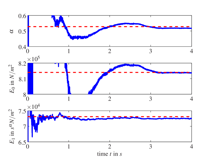
Figure 1: Identified values for $\alpha$, $E_{0}$, and $E_{1}$ (solid) compared to model parameters (dashed).

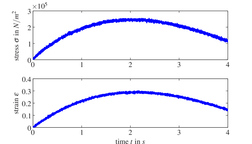
Figure 2: Trajectories of stress $\sigma$ and strain $\varepsilon$.

3.2 The general approach

In the case of homogeneous initial conditions the definitions (1) and (3) of fractional derivatives are equivalent. Therefore, without loss of generality the one due to Riemann and Liouville is used in this section.

Consider the following relation between two known signals $u$ and $y$:

$$\big{(}\bar{a}_{0}+\bar{a}_{1}D_{t}^{\bar{\alpha}_{1}}+\cdots+\bar{a}_{n}D_{t}^{\bar{\alpha}_{n}}\big{)}y(t)\\ =\big{(}\bar{b}_{0}+\bar{b}_{1}D_{t}^{\bar{\alpha}_{n+1}}+\cdots+\bar{b}_{m}D_{t}^{\bar{\alpha}_{n+m}}\big{)}u(t).$$ (18)

At least some of the parameters $\bar{a}_{i}\in\Rset$, $i=0,\dots,n$ and $\bar{b}_{i}\in\Rset$, $i=0,\dots,m$ as well as the fractional orders $\bar{\alpha}_{i}\in\Rset_{+}$, $i=1,\dots,n+m$ are considered unknown and are to be identified. Note that if all coefficients in (18) are unknown, only the coefficients in a normalized equation can be identified. Define by $\Theta$ the set of unknown parameters.

With (4a), the operational representation of (18) reads

$$\left(\bar{a}_{0}+\bar{a}_{1}s^{\bar{\alpha}_{1}}+\cdots+\bar{a}_{n}s^{\bar{\alpha}_{n}}\right)\hat{y}\\ =\left(\bar{b}_{0}+\bar{b}_{1}s^{\bar{\alpha}_{n+1}}+\cdots+\bar{b}_{m}s^{\bar{\alpha}_{n+m}}\right)\hat{u}.$$ (19)

First, the fractional operators $s^{\bar{\alpha}_{i}}$, $i=1,\dots,m+n$ are eliminated. For that, (19) is rewritten as

$$\big{(}a_{0}(s)\hat{y}-b_{0}(s)\hat{u}\big{)}s^{\alpha_{0}}+\big{(}a_{1}(s)\hat{y}-b_{1}(s)\hat{u}\big{)}s^{\alpha_{1}}\\ +\cdots+\big{(}a_{r}(s)\hat{y}-b_{r}(s)\hat{u}\big{)}s^{\alpha_{r}}=0$$ (20)

where $a_{i}(s),b_{i}(s)\in\Rset(s)$, $i=0,\dots,r$ with $r\leq n+m$ are rational in $s$. These expressions obviously involve the original parameters $\bar{a}_{i}$, $i=0,\dots,n$ and $\bar{b}_{i}$, $i=0,\dots,m$. Note that one or more of the fractional orders $\alpha_{i}$, $i=0,\dots,r$ can be integer or even zero.

As in the introductory example, (20) is derived w.r.t. $s$ a total of $r$ times. The resulting homogeneous linear system of equations for $s^{\alpha_{i}}$, $i=0,\dots,r$ has the general structure

$$\begin{pmatrix}a_{0}(s)\hat{y}-b_{0}(s)\hat{u}&\cdots&a_{r}(s)\hat{y}-b_{r}(s)\hat{u}\\[2.15277pt] p_{1,0}\!(s,\!\textstyle\frac{d}{ds}\displaystyle)\hat{y}\!-\!q_{1,0}\!(s,\!\textstyle\frac{d}{ds}\displaystyle)\hat{u}&\cdots&p_{1,r}\!(s,\!\textstyle\frac{d}{ds}\displaystyle)\hat{y}\!-\!q_{1,r}\!(s,\!\textstyle\frac{d}{ds}\displaystyle)\hat{u}\\[2.15277pt] \vdots&&\vdots\\[2.15277pt] p_{r,0}\!(s,\!\textstyle\frac{d}{ds}\displaystyle)\hat{y}\!-\!q_{r,0}\!(s,\!\textstyle\frac{d}{ds}\displaystyle)\hat{u}&\cdots&p_{r,r}\!(s,\!\textstyle\frac{d}{ds}\displaystyle)\hat{y}\!-\!q_{r,r}\!(s,\!\textstyle\frac{d}{ds}\displaystyle)\hat{u}\end{pmatrix}\\ \cdot\begin{pmatrix}s^{\alpha_{0}}\\[2.15277pt] \vdots\\[2.15277pt] s^{\alpha_{r}}\end{pmatrix}=\boldsymbol{0}$$ (21)

where $p_{i,j}(s,\textstyle\frac{d}{ds}\displaystyle),q_{i,j}(s,\textstyle\frac{d}{ds}\displaystyle)\in\Rset(s)[\textstyle\frac{d}{ds}\displaystyle]$, $i=1,\dots,r$, $j=0,\dots,r$ are polynomials in $\textstyle\frac{d}{ds}\displaystyle$ with coefficients in $\Rset(s)$. They are defined recursively by

$$p_{i,j}(s,\textstyle\frac{d}{ds}\displaystyle)=\textstyle\frac{d}{ds}\displaystyle p_{i-1,j}(s,\textstyle\frac{d}{ds}\displaystyle)+p_{i-1,j}(s,\textstyle\frac{d}{ds}\displaystyle)(\textstyle\frac{d}{ds}\displaystyle+\alpha_{j}s^{-1})$$ (22a)

$$q_{i,j}(s,\textstyle\frac{d}{ds}\displaystyle)=\textstyle\frac{d}{ds}\displaystyle q_{i-1,j}(s,\textstyle\frac{d}{ds}\displaystyle)+q_{i-1,j}(s,\textstyle\frac{d}{ds}\displaystyle)(\textstyle\frac{d}{ds}\displaystyle+\alpha_{j}s^{-1})$$ (22b)

with $p_{0,j}(s,\!\textstyle\frac{d}{ds}\displaystyle)=a_{j}(s)$ and $q_{0,j}(s,\!\textstyle\frac{d}{ds}\displaystyle)=b_{j}(s)$, $j=0,\dots,r$. Note that products $p_{i,j}(s,\!\textstyle\frac{d}{ds}\displaystyle)\hat{y}$ and $q_{i,j}(s,\!\textstyle\frac{d}{ds}\displaystyle)\hat{u}$ can also be written as sums of $\hat{y}$ and $\hat{u}$ and its derivatives with coefficients in $\Rset(s)$. Hence, the operator $\textstyle\frac{d}{ds}\displaystyle$ does not explicitly occur.

From (21) it becomes apparent that the matrix in this equation, henceforth denoted by $P$, has to be singular. Then, from $\det P=0$ an equation is obtained that involves

• (most importantly) only integer orders of $s$,

• products of $r$ operators $\hat{u}$, $\hat{y}$, and their derivatives w.r.t. $s$,

• as well as products of parameters $\bar{a}_{i}\in\Rset$, $i=0,\dots,n$ and $\bar{b}_{i}\in\Rset$, $i=0,\dots,m$ and fractional orders $\alpha_{i}\in\Rset_{+}$, $i=0,\dots,r$.

A multiplication with $s^{-k}$ with sufficiently large $k$ such that only non-positive powers of $s$ remain gives an expression of the form

$$F(s^{-1},\hat{y},\dots,\hat{y}^{(r)},\hat{u},\dots,\hat{u}^{(r)})=0,$$ (23)

where $F$ is polynomial w.r.t. to all its arguments and parameters $\Theta_{1}\subset\Theta$ including all fractional orders $\alpha_{i}$, $i=0,\dots,r$ to be identified. The knowledge of at least one of the orders is required in order to identify the others (cf. (20)) – again, this can be considered as a kind of non-restrictive normalization.

Note that the expressions occurring in (23) can easily be written as functions of time $t$ again. Hence, depending on the number of unknown (independent) coefficients in (23), which is larger or equal to the cardinality of $\Theta_{1}$, additional equations are required to solve for the parameters. They are obtained, e.g., by multiplication of (23) with negative powers of $s$. Further integration of the corresponding time functions yields independent equations for sufficiently rich signals. While other approaches of generating independent equations are possible – basically by applying other operators from $\Rset(s)[\textstyle\frac{d}{ds}\displaystyle]$ to (23) – which might exhibit a better numerical behavior or might be more suitable in the presence of noise, this is not in the focus of the present contribution. Also, the issue of whether the parameter problem arising from (23) is solved as a nonlinear equation or a linear one (by overparametrization) is not discussed here. Several approaches are well-known to the community. In the context of algebraic identification some insight into this is given in Fliess and Sira-Ramírez (2003) and Gehring et al. (2012).

It is rather obvious that parameters $\Theta_{2}\subset\Theta$ with $\Theta=\Theta_{1}\cup\Theta_{2}$ exclusively occurring as a factor of a fractionally differentiated signal in (18) or more precisely a common factor of any $a_{i}(s)\hat{y}-b_{i}(s)\hat{u}$, $i=0,\dots,r$ in (20) will not occur in (23). However, as done for the introductory example, these parameters can be calculated based on the identified values for $\Theta_{1}$ and (20).

To this end, based on estimates for the fractional orders, (20) is multiplied with $s^{-\nu}$, $\Nset\ni\nu>\max_{i}\alpha_{i}$, i.e., such that only non-positive powers of $s$ remain. Then, as before, depending on the number of parameters remaining to be identified (which corresponds to the cardinality of $\Theta_{2}$) additional equations are obtained by multiplication with negative powers of $s$. The solution of this linear system of equations completes the identification.

4 The case of inhomogeneous initial conditions

For inhomogeneous initial conditions the definitions (1) and (3) are essentially different. To illustrate this, first, the introductory example is revisited.

4.1 Introductory example

4.1.1 Riemann-Liouville fractional derivative

For inhomogeneous initial conditions the operational representation of (8) (with the Riemann-Liouville operator) reads

$$\hat{\sigma}=E_{0}\hat{\varepsilon}+E_{1}\big{(}s^{\alpha}\hat{\varepsilon}-J_{t}^{1-\alpha}\varepsilon(0)\big{)}$$ (24)

since $\alpha\in(0,1)$ and, therefore, $\nu=1$. Again, (10) results from applying $\textstyle\frac{d}{ds}\displaystyle$ to (24) and is rewritten here for completeness:

$$\hat{\sigma}^{\prime}=E_{0}\hat{\varepsilon}^{\prime}+E_{1}(\hat{\varepsilon}^{\prime}+\alpha s^{-1}\hat{\varepsilon})s^{\alpha}.$$ (25)

If the initial value $J_{t}^{1-\alpha}\varepsilon(0)$ is known, both equations can be combined such that $s^{\alpha}$ is eliminated. Similarly as in the case of homogeneous initial conditions, (25) is obtained with $\hat{\sigma}+E_{1}J_{t}^{1-\alpha}\varepsilon(0)$ instead of $\hat{\sigma}$:

$$(\hat{\varepsilon}^{\prime}+\alpha s^{-1}\hat{\varepsilon})\big{(}\hat{\sigma}+E_{1}J_{t}^{1-\alpha}\varepsilon(0)-E_{0}\hat{\varepsilon}\big{)}=\hat{\varepsilon}(\hat{\sigma}^{\prime}-E_{0}\hat{\varepsilon}^{\prime}).$$ (26)

However, since the initial value $J_{t}^{1-\alpha}\varepsilon(0)$ is not simply the value of $\varepsilon$ at $t=0$ but is more complicated to interpret, it is only plausible to consider it as unknown. As discussed in the sequel, the unknown initial values (here only one) can either be eliminated by some algebraic manipulations or they can be treated as additional parameters and included in the identification. For the present example, the latter approach simply means that there are three parameters – or products of parameters – namely $\alpha$, $E_{0}$, and $E_{1}J_{t}^{1-\alpha}\varepsilon(0)$ to be identified in (26).

On the other hand, an elimination of an unknown initial value bears the advantage of being faced with less parameters to be identified. Clearly, (25) does not depend on $\varepsilon(0)$ anymore. So deriving once more w.r.t. $s$ allows for the elimination of $s^{\alpha}$:

$$\big{(}\hat{\varepsilon}^{\prime\prime}+2\alpha s^{-1}\hat{\varepsilon}^{\prime}+\alpha(\alpha-1)s^{-2}\hat{\varepsilon}\big{)}(\hat{\sigma}^{\prime}-E_{0}\hat{\varepsilon}^{\prime})\\ =(\hat{\varepsilon}^{\prime}+\alpha s^{-1}\hat{\varepsilon})(\hat{\sigma}^{\prime\prime}-E_{0}\hat{\varepsilon}^{\prime\prime}).$$ (27)

The operational expressions in this equation can again be written as functions of time, which yields a nonlinear equation in $E_{0}$ and $\alpha$. In order to determine the unknown parameters either the nonlinear parameter problem can be solved or overparametrization can be used treating the coefficients $\alpha$, $\alpha^{2}$, $E_{0}$, $\alpha E_{0}$, and $\alpha^{2}E_{0}$ as independent.

4.1.2 Caputo fractional derivative

The approach is a little different if Caputo’s fractional derivative is used instead of the one due to Riemann and Liouville. In order to illustrate this, $D_{t}^{\alpha}$ in (8) is replaced by ${{}^{C}}\!D_{t}^{\alpha}$. The correspondence (4b) then yields

$$\hat{\sigma}=E_{0}\hat{\varepsilon}+E_{1}\big{(}s^{\alpha}\hat{\varepsilon}-\varepsilon(0)s^{\alpha-1}\big{)}.$$ (28)

As mentioned before, Caputo’s definition bears the advantage of using initial values (here $\varepsilon(0)$) that can easily be interpreted. While in this simple example the presumed knowledge of $\varepsilon(0)$ does not impose any restriction, since $\varepsilon$ itself is considered as a known signal, for $\alpha>1$ initial values of derivatives come into play that are unknown in general. For that reason, and because in a real application measurements are noisy, $\varepsilon(0)$ is assumed to be unknown in the sequel.

Deriving (28) w.r.t. $s$ gives

$$\hat{\sigma}^{\prime}=E_{0}\hat{\varepsilon}^{\prime}+E_{1}\big{(}s^{\alpha}(\hat{\varepsilon}^{\prime}+\alpha s^{-1}\hat{\varepsilon})-(\alpha-1)s^{-1}\varepsilon(0)s^{\alpha-1}\big{)}.$$ (29)

If the initial value is to be identified, eliminating $s^{\alpha}$ from (29) using (28),

$$(\hat{\sigma}^{\prime}\hat{\varepsilon}-\hat{\sigma}\hat{\varepsilon}^{\prime})=\big{(}\varepsilon(0)(1-\alpha)s^{-2}+\alpha s^{-1}\hat{\varepsilon}\big{)}(\hat{\sigma}-E_{0}\hat{\varepsilon})\\ +\varepsilon(0)s^{-1}(\hat{\sigma}^{\prime}-E_{0}\hat{\varepsilon}^{\prime})$$ (30)

is obtained which is an equation of the type (23) and involves the parameters $\varepsilon(0)$, $E_{0}$, and $\alpha$.

Alternatively, the initial value $\varepsilon(0)$ can simply be eliminated by multiplying (28) with $(1-\alpha)s^{-1}$ and adding it to (29) multiplied with $s$:

$$(1-\alpha)\hat{\sigma}+s\hat{\sigma}^{\prime}=E_{0}(1-\alpha)\hat{\varepsilon}+E_{0}s\hat{\varepsilon}^{\prime}+E_{1}s^{\alpha}(\hat{\varepsilon}+s\hat{\varepsilon}^{\prime}).$$ (31)

By taking yet another derivative of this equation w.r.t. $s$ the factor $s^{\alpha}$ corresponding to the fractional derivative is replaced. Multiplying with $s^{-2}$, the resulting equation

$$\hat{\sigma}^{\prime}\hat{\varepsilon}^{\prime\prime}-\hat{\sigma}^{\prime\prime}\hat{\varepsilon}^{\prime}+s^{-1}(\hat{\sigma}\hat{\varepsilon}^{\prime\prime}-\hat{\sigma}^{\prime\prime}\hat{\varepsilon})+2s^{-2}(\hat{\sigma}\hat{\varepsilon}^{\prime}-\hat{\sigma}^{\prime}\hat{\varepsilon})\\ =\alpha s^{-2}(\hat{\sigma}\hat{\varepsilon}^{\prime}-\hat{\sigma}^{\prime}\hat{\varepsilon})-\alpha s^{-1}(2\hat{\varepsilon}^{\prime}+s^{-1}\hat{\varepsilon})(\hat{\sigma}^{\prime}-E_{0}\hat{\varepsilon}^{\prime})\\ +\alpha s^{-1}\big{(}\hat{\varepsilon}^{\prime\prime}+\alpha s^{-1}\hat{\varepsilon}^{\prime}+(\alpha-1)s^{-2}\hat{\varepsilon}\big{)}(\hat{\sigma}-E_{0}\hat{\varepsilon})$$ (32)

is of the type (23) and involves the parameters $E_{0}$ and $\alpha$.

4.2 The general approach

Based on the previous example and the discussions in section 3.2 for the homogeneous case the general approach for an equation (18) is rather obvious. That is why only a sketch is given of how to obtain relations of the form (23). For both the Riemann-Liouville and the Caputo definition the cases where initial conditions are eliminated and the one where they are identified are treated. Henceforth, it is assumed that an upper bound of all unknown (integer or fractional) orders $\bar{\alpha}_{i}$, $i=1,\dots,n+m$ is available.

4.2.1 Riemann-Liouville fractional derivative

For a known upper bound $\nu\in\Nset$ of the order of differentiation, the operational representation of (18) (corresponding to (20) for homogeneous initial conditions) can be written as

$$\big{(}a_{0}(s)\hat{y}-b_{0}(s)\hat{u}\big{)}s^{\alpha_{0}}+\big{(}a_{1}(s)\hat{y}-b_{1}(s)\hat{u}\big{)}s^{\alpha_{1}}\\ +\cdots+\big{(}a_{r}(s)\hat{y}-b_{r}(s)\hat{u}\big{)}s^{\alpha_{r}}=\textstyle\sum_{i=1}^{\nu}c_{i}s^{i-1}$$ (33)

where the coefficients $c_{i}$, $i=0,\dots,\nu$ depend on initial values of $u$ and $y$ and their derivatives as well as parameters $\bar{a}_{i}$, $0,\dots,n$ and $\bar{b}_{i}$, $i=0,\dots,m$. Applying $\textstyle\frac{d}{ds}{}^{\nu}$ to this equations eliminates all these initial values. Following the elimination of the fractional operators $s^{\alpha_{i}}$, $i=0,\dots,r$, a multiplication with $s^{-k}$ (with sufficiently large $k$) yields an equation of the form (23) with $r+\nu$ instead of $r$.

On the other hand, identifying the initial values – even though they lack physical meaning – is almost identical to the procedure in section 3.2, the only difference being that (21) is inhomogeneous with the right hand side of the equation being a vector of polynomials in $s$. Using the solution of this linear problem and substituting it in an additional equation involving the fractional orders $s^{\alpha_{i}}$ (generated from deriving once more w.r.t. $s$), again, a multiplication with a sufficiently large negative power of $s$ results in (23).

4.2.2 Caputo fractional derivative

The operational representation of (18) with Caputo’s derivation operator gives

$$\big{(}a_{0}(s)\hat{y}-b_{0}(s)\hat{u}-\textstyle\sum_{i=1}^{\nu}c_{0,i}s^{-i}\big{)}s^{\alpha_{0}}\\ +\cdots+\big{(}a_{r}(s)\hat{y}-b_{r}(s)\hat{u}-\textstyle\sum_{i=1}^{\nu}c_{r,i}s^{-i}\big{)}s^{\alpha_{r}}=0$$ (34)

for a known upper bound $\nu\in\Nset$. The coefficients $c_{i,j}$, $i=0,\dots,r$, $j=1,\dots,\nu$ can be cancelled by taking a sufficient number of derivatives w.r.t. $s$ and solving the resulting linear system of equations for these coefficients. Afterwards, an expression of the form (23) can be obtained using $r$ further differentiations of this result and multiplying it with a sufficiently large negative power of $s$.

If, however, one is interested in the initial values, as in the homogeneous case, the fractional operators $s^{\alpha_{i}}$ in (34) can simply be eliminated by taking $r$ derivatives and calculating the solution of this linear system (cf. (21)).

5 Linear partial differential equations with fractional derivatives

The identification of fractional orders and model parameters discussed for lumped fractional models can be extended to fractional distributed parameter systems. For the integer order case, Rudolph and Woittennek (2008) and Gehring et al. (2012) demonstrated that based on the knowledge of the solution of the corresponding operational ordinary differential equation a relation of the form (23) between two boundary measurements can be obtained.

Here, the basic ideas of the identification method are demonstrated on an example. Since homogeneous initial conditions are assumed, without loss of generality, only the Riemann-Liouville fractional derivative is used.

The example considered is the fractional diffusion-wave equation (see e.g. Mainardi (1997); Podlubny (1999))

$$v^{2}D_{z}^{2}u(z,t)=D_{t}^{\alpha}u(z,t),\qquad(z,t)\in\Rset_{+}^{2}$$ (35)

with $v\in\Rset$, where the derivative w.r.t. time is of fractional order $\alpha\in(0,2]$. The factor $v^{2}$ is the diffusion coefficient for $\alpha=1$, and it is the squared wave propagation speed for $\alpha=2$. In the context of signal propagation as addressed in Mainardi (1997) the boundary conditions are

$$u(0,t)=h(t),\qquad u(\infty,t)=0.$$ (36)

Additionally, as mentioned before, homogeneous initial conditions are assumed.

The operational representation of (35) reads

$$v^{2}D_{z}^{2}\hat{u}(z)=s^{\alpha}\hat{u}(z)$$ (37)

and is a second order ordinary differential equation w.r.t. $z$ that can easily be solved. From the general solution

$$\hat{u}(z)=\hat{C}_{1}\mathrm{e}^{\frac{z}{v}s^{\alpha/2}}+\hat{C}_{2}\mathrm{e}^{-\frac{z}{v}s^{\alpha/2}}$$ (38)

using the (operational form) of the boundary conditions (36) yields operators $\hat{C}_{1}=0$ and $\hat{C}_{2}=\hat{h}$.

In order to identify the fractional order $\alpha$, apart from the knowledge of $h$, another measurement is required. If $u$ is measured at some point $z=L\neq 0$, such that $g(t)=u(L,t)$ is known, (38) gives

$$\hat{g}=\hat{h}\mathrm{e}^{-\frac{L}{v}s^{\alpha/2}}.$$ (39)

Since the exponential function satisfies a first order differential equation it can be eliminated by deriving (39),

$$\hat{g}^{\prime}=\left(\hat{h}^{\prime}-\tfrac{\alpha}{2}\tfrac{L}{v}s^{-1}s^{\alpha/2}\hat{h}\right)\mathrm{e}^{-\frac{L}{v}s^{\alpha/2}}$$ (40)

and replacing the exponential function using (39):

$$\hat{g}\hat{h}^{\prime}-\hat{g}^{\prime}\hat{h}=\tfrac{\alpha}{2}\tfrac{L}{v}s^{-1}s^{\alpha/2}\hat{g}\hat{h}.$$ (41)

Finally, $s^{\alpha/2}$ is eliminated using the derivative of (41) w.r.t. $s$. The interpretation of

$$\hat{g}^{2}\big{(}(\hat{h}^{\prime})^{2}-s^{-1}\hat{h}\hat{h}^{\prime}-\hat{h}\hat{h}^{\prime\prime}\big{)}-\hat{h}^{2}\big{(}(\hat{g}^{\prime})^{2}-s^{-1}\hat{g}\hat{g}^{\prime}-\hat{g}\hat{g}^{\prime\prime}\big{)}\\ =\frac{\alpha}{2}s^{-1}\hat{g}\hat{h}(\hat{g}^{\prime}\hat{h}-\hat{g}\hat{h}^{\prime})$$ (42)

in terms of functions of time is omitted for brevity. It involves nested convolutions of known signals only. However, as can clearly be seen, (42) constitutes a linear equation in $\alpha$. Based on an estimated value for the fractional order, the quotient $L/v$ can directly be calculated from (41) (since $s^{\alpha/2-1}$ already corresponds to a fractional integral for $\alpha\in(0,2)$).

6 Conclusion

Using the algebraic framework presented model parameters and fractional (as well as integer) orders can be identified in linear fractional models. The exact relations obtained for the unknown quantities involve only convolutions of known (input and output) signals. Based on positive results using simulation data, the authors intend to further validate the identification algorithms using experimental data. In this context numerical aspects related to online implementation and robustness w.r.t. measurement noise should be investigated.

The example of the fractional diffusion-wave equation demonstrates, that the method is also applicable to (at least certain) linear fractional distributed parameter systems as well as delay systems with fractional derivatives. Beyond that, an extension towards the identification of the structure of linear systems, i.e., ordinary differential equations, seems possible where, both, the order of the equations and their coefficients can be estimated.

References

- Bagley (1983) R.L. Bagley. A theoretical basis for the application of fractional calculus to viscoelasticity. J. Rheol., 27(3):201–210, 1983.
- Cois et al. (2001) O. Cois, A. Oustaloup, T. Poinot, and J.-L. Battaglia. Fractional state variable filter for system identification by fractional model. In Proc. 6th European Control Conference (ECC’2001), September 2001.
- Fliess and Sira-Ramírez (2003) M. Fliess and H. Sira-Ramírez. An algebraic framework for linear identification. ESAIM: Control, Optimisation and Calculus of Variations, 9:151–168, 2003.
- Gehring et al. (2012) N. Gehring, T. Knüppel, J. Rudolph, and F. Woittennek. Algebraic identification of heavy rope parameters. In Proc. 16th IFAC Symposium on System Identification, pages 161–166, July 2012.
- Gorenflo and Mainardi (1997) R. Gorenflo and F. Mainardi. Fractional calculus: integral and differential equations of fractional order. In A. Carpinteri and F. Mainardi, editors, Fractals and Fractional Calculus in Continuum Mechanics, pages 223–276. Springer-Verlag, 1997.
- Hotzel and Fliess (1998) R. Hotzel and M. Fliess. On linear systems with a fractional derivation: Introductory theory and exmaples. Math. Comput. Simul., 45:385–395, 1998.
- Kim and Lee (2009) S.-Y. Kim and D.-H. Lee. Identification of fractional-derivative-model parameters of viscoelastic materials from measured FRFs. J. Sound Vib., 324:570–586, 2009.
- Lorenzo and Hartley (2008) C.F. Lorenzo and T.T. Hartley. Initialization of fractional-order operators and fractional differential equations. J. Comput. Nonlinear Dynam., 3:021101, 2008.
- Mainardi (1997) F. Mainardi. Fractional calculus: some basic problems in continuum and statistical machanics. In A. Carpinteri and F. Mainardi, editors, Fractals and Fractional Calculus in Continuum Mechanics, pages 291–348. Springer-Verlag, 1997.
- Malti et al. (2007) R. Malti, S. Victor, V. Nicolas, and A. Oustaloup. System identification using fractional models: State of the art. In Proc. ASME 2007 International Design Engineering Technical Conferences and Computers and Information in Engineering Conference (IDETC/CIE2007), pages 295–304, September 2007.
- Mikusiński (1983) J. Mikusiński. Operational Calculus. Pergamon, Oxford & PWN, 1983.
- Oldham and Spanier (1974) K.B. Oldham and J. Spanier. The Fractional Calculus. Academic Press, 1974.
- Podlubny (1999) I. Podlubny. Fractional Differential Equations. Academic Press, 1999.
- Rudolph and Woittennek (2008) J. Rudolph and F. Woittennek. An algebraic approach to parameter identification in linear infinite dimensional systems. In Proc. 16th Mediterranean Conference on Control and Automation, pages 332–337, June 2008.
- Schmidt and Gaul (2002) A. Schmidt and L. Gaul. Application of fractional calculus to viscoelastically damped structures in the finite element method. In Proc. Int. Conf. on Structural Dynamics Modelling (SDM), pages 297–306, June 2002.
- Torvik and Bagley (1984) P.J. Torvik and R.L. Bagley. On the appearance of the fractional derivative in the behavior of real materials. J. Appl. Mech., 51:294–298, 1984.
- Trigeassou et al. (2012) J.C. Trigeassou, N. Maamri, J. Sabatier, and A. Oustaloup. Transients of fractional-order integrator and derivatives. Signal, Image and Video Processing, 60:1–14, 2012.