Quantitative Study
of Different Forms of Geometrical Scaling
in Deep Inelastic Scattering at HERA

Abstract

We use recently proposed method of ratios to assess the quality of geometrical scaling in deep inelastic scattering for different forms of the saturation scale. We consider original form of geometrical scaling (motivated by the Balitski-Kovchegov (BK) equation with fixed coupling) studied in more detail in our previous paper, and four new hypotheses: phenomenologically motivated case with $Q^{2}$ dependent exponent $\lambda$ that governs small $x$ dependence of the saturation scale, two versions of scaling (running coupling 1 and 2) that follow from the BK equation with running coupling, and diffusive scaling suggested by the QCD evolution equation beyond mean field approximation. It turns out that more sophisticated scenarios: running coupling scaling and diffusive scaling are disfavored by the combined HERA data on $e^{+}p$ deep inelastic structure function $F_{2}$.

1 Introduction

Geometrical scaling (GS) has been introduced in Ref. Stasto:2000er in the context of low $x$ Deep Inelastic Scattering (DIS). It has been conjectured that $\gamma^{\ast}p$ cross-section $\sigma_{\gamma^{\ast}p}(x,Q^{2})=4\pi^{2}\alpha_{\mathrm{em}}F_{2}(x,Q^{2})/Q^{2}$ which in principle depends on two independent kinematical variables $Q^{2}$ and $W$ (i.e. $\gamma^{\ast}p$ scattering energy), depends only on a specific combination of them, namely upon

$$\tau=\frac{Q^{2}}{Q_{\text{s}}^{2}(x)}$$ (1)

called scaling variable. Bjorken $x$ variable is defined as

$$x=\frac{Q^{2}}{Q^{2}+W^{2}-M_{\text{p}}^{2}}$$ (2)

and $M_{p}$ denotes the proton mass. In Ref. Stasto:2000er , following Golec-Biernat–Wüsthoff (GBW) model GolecBiernat:1998js , function $Q_{\text{s}}(x)$ – called saturation scale – was taken in the following form

$$Q_{\text{s}}^{2}(x)=Q_{0}^{2}\left(\frac{x}{x_{0}}\right)^{-\lambda}.$$ (3)

Here $Q_{0}$ and $x_{0}$ are free parameters which can be extracted from the data within some specific model of DIS, and exponent $\lambda$ is a dynamical quantity of the order of $\lambda\sim 0.3$. In the GBW model $Q_{0}=1~{}$GeV$/c$ and $x_{0}=3\times 10^{-4}.$

In our previous paper Praszalowicz:2012zh (see also Stebel:2012ky ) we have proposed a simple method of ratios to assess in the model independent way the quality and the range of applicability of GS for the saturation scale defined in Eq. (3). Here we follow the same steps to test four different forms of the saturation scale that have been proposed in the literature.

Geometrical scaling is theoretically motivated by the gluon saturation phenomenon (for review see Refs. Mueller:2001fv ; McLerran:2010ub ) in which low $x$ gluons of given transverse size $\sim 1/Q^{2}$ start to overlap and their number is no longer growing once $Q^{2}$ is decreased. This phenomenon – called gluon saturation – appears formally due to the nonlinearities of parton evolution at small $x$ given by so called JIMWLK hierarchy equations jimwlk which in the large $N_{\rm c}$ limit reduce to the Balitsky-Kovchegov equation BK . These equations admit traveling wave solutions which explicitly exhibit GS Munier:2003vc . An effective theory describing small $x$ regime is Color Glass Condensate sat1 ; MLV .

Gluon saturation takes place for Bjorken $x$ much smaller than 1. Yet in Ref. Praszalowicz:2012zh we have shown that GS with saturation scale defined by Eq. (3) works very well up to much higher values of $x$, namely up to $x\sim 0.1$. In this region GS cannot be attributed to the saturation physics alone. Indeed, it is known that GS scaling extends well above the saturation scale both in the Dokshitzer-Gribov-Lipatov–Altarelli-Parisi DGLAP (DGLAP) Kwiecinski:2002ep and Balitsky-Lipatov-Fadin-Kuraev BFKL (BFKL) Iancu:2002tr evolution schemes once the boundary conditions satisfy GS to start with. It has been also shown that in DGLAP scheme GS builds up during evolution for generic boundary conditions Caola:2008xr . Therefore in the kinematical region far from the saturation regime where, however, no other scales exist (e.g. for nearly massless particles) it is still the saturation scale which governs the behavior of the $\gamma^{\ast}p$ cross-section.

The form of saturation scale given by Eq.(3) is dictated by the asymptotic behavior Munier:2003vc of the Balitsky-Kovchegov (BK) equation BK , which is essentially the BFKL equation BFKL supplied with a nonlinear damping term. It has been first used in the papers by K. Golec-Biernat and M. Wüsthoff GolecBiernat:1998js where the saturation model of inclusive and diffractive DIS has been formulated and tested phenomenologically.

Since the original discovery of GS in 2001 there have been many theoretical attempts to find a ”better” scaling variable which is both theoretically justified and phenomenologically acceptable. An immediate generalization of the saturation model of Refs. GolecBiernat:1998js has been done in Ref. Bartels:2002cj where DGLAP DGLAP evolution in $Q^{2}$ has been included. Although the exact formulation of DGLAP improved saturation model requires numerical solution of DGLAP equations, one can take this into account phenomenologically by allowing for an effective $Q^{2}$ dependence of the exponent $\lambda=\lambda_{\rm phn}(Q^{2})$ which is indeed seen experimentally in the low $x$ behavior of $F_{2}$ structure function (see e.g. Refs. Bartels:2002cj ; Kowalski:2010ue and Fig. 1). This piece of data can be relatively well described by the linear dependence of $\lambda_{\rm phn}(Q^{2})$ on $\log Q^{2}$ leading to the scaling variable of the following form

$$\tau_{\text{phn}}=Q^{2}x^{\lambda_{0}+\beta\log Q^{2}/Q_{\beta}^{2}}$$ (4)

In another approach to DIS at low $x$ one considers modifications of BK equation through an inclusion of the running coupling constant effects. Depending on the approximations used two different forms of scaling variable have been discussed in the literature Munier:2003vc :

$$\tau_{\text{rc1}}=Q^{2}e^{{-\mu\sqrt{\log\left(1/x\right)}}}$$ (5)

and Beuf:2008mb

$$\tau_{\text{rc2}}=Q^{2}x^{\nu/\log(Q^{2}/Q_{\nu}^{2})}$$ (6)

where subscripts ”rc” refer to ”running coupling”. Note that from phenomenological point of view (6) is in fact a variation of (4) where a different form of $Q^{2}$ dependence has been used. Finally, generalization of the BK equation beyond a mean-field approximation leads to so called diffusive scaling DiffScal characterized by yet another scaling variable:

$$\tau_{\text{ds}}=\left(Q^{2}\right)^{1/\sqrt{\log(1/x)}}e^{-\kappa\sqrt{\log\left(1/x\right)}}.$$ (7)

These different forms of scaling variable (except (4)) have been tested in a series of papers Gelis:2006bs ; Beuf:2008bb ; Royon:2010tz where the so called Quality Factor (QF) has been defined and used as a tool to assess the quality of geometrical scaling. In the following we shall use the method developed in Refs. Praszalowicz:2012zh ; Stebel:2012ky to test hypothesis of GS in scaling variables (4)–(7) and to study the region of its applicability using combined analysis of $e^{+}p$ HERA data HERAcombined . We shall also compare our results with earlier findings of Refs.Gelis:2006bs ; Beuf:2008bb ; Royon:2010tz .

Our results can be summarized as follows: more sophisticated scenarios i.e. running coupling scaling and diffusive scaling are disfavored by the combined HERA data on $e^{+}p$ deep inelastic structure function $F_{2}$. In contrast, phenomenologically motivated case with $Q^{2}$ dependent exponent $\lambda$ and the originally proposed form of the saturation scale Stasto:2000er with fixed $\lambda$ exhibit high quality geometrical scaling over the large region of Bjorken $x$ up to 0.1. The fact that GS is valid up to much larger Bjorken $x$’s than originally anticipated has been already used in an analysis of GS in the multiplicity $p_{\rm T}$ spectra in $pp$ collisions Praszalowicz:2013uu .

In Sect. 2 we briefly recapitulate the method of ratios of Ref. Praszalowicz:2012zh and define the criteria for GS to hold. In Sect. 3 we present results for 4 different scaling variables introduced in Eqs.(4)–(7). Finally in Sect. 4 we compare these results with our previous paper Praszalowicz:2012zh and with the results of Refs. Gelis:2006bs ; Beuf:2008bb ; Royon:2010tz .

2 Method of ratios

Throughout this paper we shall use model-independent method used in Refs. Stebel:2012ky ; Praszalowicz:2012zh which was developed in Refs.GSinpp to test GS in multiplicity distributions at the LHC. Geometrical scaling hypothesis means that

$$\sigma_{\gamma^{\ast}p}(x_{i},Q^{2})=\frac{1}{Q_{0}^{2}}F(\tau)$$ (8)

where for simplicity we define $\sigma_{\gamma^{\ast}p}$ as

$$\sigma_{\gamma^{\ast}p}(x_{i},Q^{2})=\frac{F_{2}(x_{i},Q^{2})}{Q^{2}}.$$ (9)

Function $F$ in Eq. (8) is a universal dimensionless function of $\tau$. In view of Eq. (8) cross-sections $\sigma_{\gamma^{\ast}p}(x_{i},Q^{2})$ for different $x_{i}$’s, evaluated not in terms of $Q^{2}$ but in terms of $\tau$, should fall on one universal curve. This means in turn that if we calculate ratio of cross-sections for different Bjorken $x_{i}$’s, each expressed in terms of $\tau$, we should get unity independently of $\tau$. This allows to determine parameter governing $x$ dependence of $\tau$ by minimizing deviations of these ratios from unity. Generically we denote this parameter as $\alpha$, although for each scaling variable (4) – (7) it has a different meaning: $\alpha=\beta,\,\mu,\,\nu$ and $\kappa$ for $Q^{2}$-dependent, running coupling (1 and 2) and diffusive scaling hypotheses, respectively.

Following Stebel:2012ky ; Praszalowicz:2012zh we apply here the following procedure. First we choose some $x_{\mathrm{ref}}$ and consider all Bjorken $x_{i}$’s smaller than $x_{\mathrm{ref}}$ that have at least two overlapping points in $Q^{2}$ (or more precisely in scaling variable $\tau$). Next we form the ratios

$$R_{x_{i},x_{\text{ref}}}(\alpha;\tau_{k})=\frac{\sigma_{\gamma^{\ast}p}(x_{i},\tau(x_{i},Q_{k}^{2};\alpha))}{\sigma_{\gamma^{\ast}p}(x_{\text{ref}},\tau(x_{\text{ref}},Q_{k,\text{ref}}^{2};\alpha))}$$ (10)

with

$$\tau_{k}=\tau(x_{i},Q_{k}^{2};\alpha)=\tau(x_{\text{ref}},Q_{k,\text{ref}}^{2};\alpha).$$ (11)

By tuning $\alpha$ one can make $R_{x_{i},x_{\text{ref}}}(\alpha;\tau_{k})=1\pm\delta$ for all $\tau_{k}$ with accuracy of $\delta$ for which following Ref. Praszalowicz:2012zh we take 3%.

For $\alpha\neq 0$ points of the same $Q^{2}$ but different $x$’s correspond generally to different $\tau$’s. Therefore one has to interpolate the reference cross-section $\sigma_{\gamma^{\ast}p}(x_{\text{ref}},\tau(x_{\text{ref}},Q^{2};\alpha))$ to $Q_{k,\text{ref}}^{2}$ such that $\tau(x_{\text{ref}},Q_{k,\text{ref}}^{2};\alpha)=\tau_{k}$ as indicated in Eq. (11). This procedure is described in detail in Refs. Praszalowicz:2012zh ; Stebel:2012ky .

In order to find optimal value of parameter $\alpha$ that minimizes deviations of ratios (10) from unity we form the chi-square measure

$$\chi_{x_{i},x_{\text{ref}}}^{2}(\alpha)=\frac{1}{N_{x_{i},x_{\text{ref}}}-1}{\displaystyle\sum\limits_{k\in x_{i}}}\frac{\left(R_{x_{i},x_{\text{ref}}}(\alpha;\tau_{k})-1\right)^{2}}{\Delta R_{x_{i},x_{\text{ref}}}(\alpha;\tau_{k})^{2}}$$ (12)

where the sum over $k$ extends over all points of given $x_{i}$ that have overlap with $x_{\text{ref}}$ and ${N_{x_{i},x_{\text{ref}}}}$ is a number of such points.

Finally, the errors entering formula (12) are calculated using

$$\Delta R_{x_{i},x_{\text{ref}}}(\alpha;\tau_{k})^{2}=$$ (13)

$$\left(\left(\frac{\Delta\sigma_{\gamma^{\ast}p}(x_{i},\tau(x_{i},Q_{k}^{2}))}{\sigma_{\gamma^{\ast}p}(x_{i},\tau(x_{i},Q_{k}^{2}))}\right)^{2}+\left(\frac{\Delta\sigma_{\gamma^{\ast}p}(x_{\text{ref}},\tau(x_{\text{ref}},Q_{k,\text{ref}}^{2}))}{\sigma_{\gamma^{\ast}p}(x_{\text{ref}},\tau(x_{\text{ref}},Q_{k,\text{ref}}^{2}))}\right)^{2}\right)R_{x_{i},x_{\text{ref}}}(\alpha;\tau_{k})^{2}+\delta^{2}$$

where $\Delta\sigma_{\gamma^{\ast}p}(\tau(x,Q^{2}))$ are experimental errors (or interpolated experimental errors) of $\gamma^{\ast}p$ cross-sections (9). For more detailed discussion of errors see Ref. Praszalowicz:2012zh .

In this way, for each pair of available Bjorken variables $(x_{i},x_{\mathrm{ref}})$, we compute the best value of parameter $\alpha$, denoted in the following by a subscript min: $\alpha_{\mathrm{min}}(x_{i},x_{\mathrm{ref}})$ and the corresponding $\chi^{2}$. For GS to hold we should find a region in $(x_{i},x_{\mathrm{ref}})$ half-plane (note that by construction $x_{i}<x_{\mathrm{ref}}$) where $\alpha_{\mathrm{min}}(x_{i},x_{\mathrm{ref}})$ is a constant independent of $x_{i}$ and $x_{\mathrm{ref}}$, and the corresponding $\chi_{x_{i},x_{\mathrm{ref}}}^{2}$ is small.

We shall also look for possible violations of GS in a more quantitative way. In order to eliminate the dependence of $\alpha_{\text{min}}(x,x_{\mathrm{ref}})$ on the value of $x$, we introduce averages over $x$ (denoted in the following by $\left\langle\ldots\right\rangle$) minimizing the following chi-square function:

$$\tilde{\chi}_{x_{\text{ref}}}^{2}(\left\langle\alpha\right\rangle)=\frac{1}{N_{x_{\mathrm{ref}}}-1}{\displaystyle\sum\limits_{x<x_{\text{ref}}}}\frac{\left(\alpha_{\text{min}}(x,x_{\text{ref}})-\left\langle\alpha\right\rangle\right)^{2}}{\Delta\alpha_{\text{min}}(x,x_{\text{ref}})^{2}}$$ (14)

which gives the best value of $\langle\alpha\rangle$ denoted as $\langle\alpha_{\mathrm{min}}(x_{\text{ref}})\rangle$. The sum in (14) extends over all $x$’s such that $\alpha_{\text{min}}(x,x_{\text{ref}})$ exists and $N_{x_{\mathrm{ref}}}$ is the number of terms in (14).

Since GS is expected to work for small $x$’s, the ”average” value of scaling parameter $\langle\alpha_{\mathrm{min}}(x_{\text{ref}})\rangle$ supplies an information, up to what value of $x_{\mathrm{ref}}$ GS is still working. For small $x_{\mathrm{ref}}$ we expect $\langle\alpha_{\mathrm{min}}(x_{\text{ref}})\rangle$ to be constant, whereas for larger values we expect to see some dependence of $\langle\alpha_{\mathrm{min}}(x_{\text{ref}})\rangle$ on $x_{\mathrm{ref}}$. A word of warning is here in order. Even if $\langle\alpha_{\mathrm{min}}(x_{\text{ref}})\rangle$ is a constant we have to look at the corresponding value of $\chi^{2}$: too large $\chi^{2}$ obviously indicates violation of GS.

To quantify further the hypothesis of geometrical scaling we form yet another chi-square function

$$\overline{\chi}_{x_{\text{cut}}}^{2}(\left\langle\left\langle\alpha\right\rangle\right\rangle)=\frac{1}{N_{x_{\text{cut}}}-1}{\displaystyle\sum\limits_{x_{\text{ref}}\leq x_{\text{cut}}}}\,{\displaystyle\sum\limits_{x<x_{\text{ref}}}}\frac{\left(\alpha_{\text{min}}(x,x_{\text{ref}})-\left\langle\left\langle\alpha\right\rangle\right\rangle\right)^{2}}{\Delta\alpha_{\text{min}}(x,x_{\text{ref}})^{2}}$$ (15)

which we minimize to obtain $\left\langle\left\langle\alpha_{\text{min}}(x_{\text{cut}})\right\rangle\right\rangle$.

Equation (15) allows us to see how well one can fit $\left\langle\alpha_{\text{min}}(x_{\text{ref}})\right\rangle$ with a constant $\alpha$ up to $x_{\text{ref}}=x_{\text{cut}}$. Were there any strong violations of GS above some $x_{0}$, one should see a rise of $\left\langle\left\langle\alpha_{\text{min}}(x_{\text{cut}})\right\rangle\right\rangle$ once $x_{\text{cut}}$ becomes larger than $x_{0}$.

3 Results

Let us now come back to the discussion of different scaling variables defined in Eqs. (4) – (7). All of them depend on one variational parameter, which we constrain analyzing ratios (10) for combined HERA $e^{+}p$ DIS data HERAcombined .

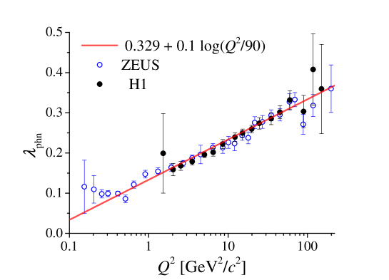
Figure 1: Effective exponent $\lambda_{\rm phn}$ from $F_{2}$ at low $x$ (17) from HERA and the linear fit of Eq. (18). Data points as in Ref. Bartels:2002cj , see also Kowalski:2010ue .

In the case of $Q^{2}$-dependent exponent $\lambda_{\rm phn}$ (4), however, there are in fact two parameters, one of them ($\lambda_{0}$) being fixed using our previous analysis of Ref. Praszalowicz:2012zh where we have shown that GS scaling works very well with constant $\lambda=\lambda_{0}$:

$$\lambda_{0}=0.329\pm 0.002.$$ (16)

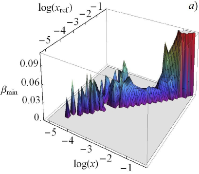
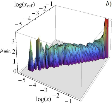
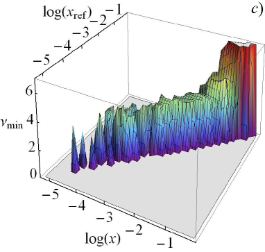
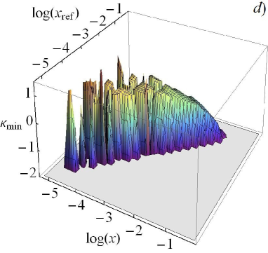
Figure 2: Three dimensional plots of a) $\beta_{\rm min}(x,x_{\rm ref})$, b) $\mu_{\rm min}(x,x_{\rm ref})$, c) $\nu_{\rm min}(x,x_{\rm ref})$ and d) $\kappa_{\rm min}(x,x_{\rm ref})$ obtained by minimizing $\chi^{2}$ function of Eq. (12).

On the other hand looking at low $x$ behavior of the $F_{2}$ structure function it has been shown that Bartels:2002cj ; Kowalski:2010ue :

$$F_{2}(x,Q^{2})\sim x^{-\lambda_{\rm phn}(Q^{2})}$$ (17)

where $\lambda_{\rm phn}(Q^{2})$ can be well parametrized as

$$\lambda_{\rm phn}(Q^{2})=0.329+0.1\log(Q^{2}/90)$$ (18)

(for $Q^{2}$ in (GeV/$c)^{2}$) as depicted in Fig. 1. Taking therefore scaling variable in the form of (4) with $\lambda_{0}=0.329$ we test in fact consistency of the slopes $\beta$ as extracted from Fig. 1 and by the procedure described in Sect. 2. Note that this is therefore a kind of perturbative two parameter fit, and as such it has a different status than the remaining Ansätze for the scaling variable (5) – (7). Similar remarks apply to the running coupling rc2 case (6), where the scale of the logarithm $Q_{\nu}^{2}$ has been fixed at $0.04$ (following e.g. Ref. Beuf:2008bb ). Then for all points $Q^{2}>Q_{\nu}^{2}$ and $\tau_{\text{rc2}}$ decreases with rising $\nu$.

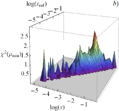
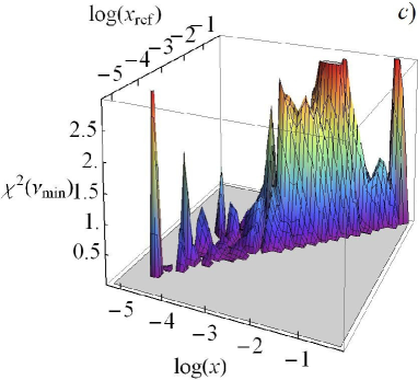
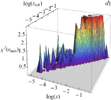
Figure 3: Three dimensional plots of minimal values of $\chi^{2}$ functions (12) for different scaling variables: a) logarithmic scaling variable $\tau_{\text{phn}}$ (4), running coupling b) rc1 (5), c) rc2 (6) and d) diffusive scaling (7).

Let us first examine 3 dimensional plots of $\alpha_{\text{min}}(x,x_{\text{ref}})$ (note again that $\alpha=\beta,\,\mu,\,\nu$ or $\kappa,$ depending on the scaling variable). For GS to hold there should be a visible plateau of $\alpha_{\text{min}}$ over some relatively large part of $(x,x_{\text{ref}})$ space (recall that by construction $x<x_{\text{ref}}$). Looking at Fig. 2 one has to remember that the values of $\alpha_{\text{min}}(x,x_{\text{ref}})$ are subject to fluctuations that will be ”averaged over” when we discuss more ”integrated” quantities $\left\langle\alpha_{\text{min}}\right\rangle$ and $\left\langle\left\langle\alpha_{\text{min}}\right\rangle\right\rangle$. Note that statistical errors of $\alpha_{\text{min}}(x,x_{\text{ref}})$ which are quite large for small $x$ are not displayed in Fig. 2. One can can conclude from Fig. 2 that for all 4 cases (4) – (7) there is rather strong dependence of $\alpha_{\text{min}}(x,x_{\text{ref}})$ for large values of $x$ and $x_{\text{ref}}$. In the case of $Q^{2}$-dependent scaling variable (4) (Fig. 2.a) and for the running coupling case (5,6) (Figs. 2.b, c), the values of parameters $\beta$, $\mu$ and $\nu$ rise steeply for large $x$’s, whereas for diffusive scaling parameter $\kappa$ is falling down rapidly. More closer look reveals that for running coupling rc1 case (Fig. 2.b) there is in fact no distinct plateau, one can also see a systematic rise of $\mu_{\text{min}}$ in a region of very small $x$’s. Similarly for the diffusive scaling (Fig. 2.d) we see rather systematic growth of $\kappa_{\text{min}}$ for small $x$’s with possible plateau in a small corner of very low $x$’s. At first glance no plateau is neither seen for $\beta_{\text{min}}(x,x_{\text{ref}})$ (Fig. 2.a). However – as will be shown in the following – because of considerable statistical uncertainties within the scale used in Fig. 2.a, very good description of GS with constant $\beta$ is still possible.

It is interesting to look at 3 dimensional plots of the corresponding $\chi^{2}$ values (12) shown in Fig. 3. Recal that for GS to hold one should observe small values of $\chi^{2}(\alpha_{\text{min}})$ in the same region where $\alpha_{\text{min}}$ is constant. This happens for $\tau_{\rm phn}$ (Fig. 3.a) where $\chi^{2}$ oscillates around 1 not exceeding 2 even for large values of $x$. Similarly $\tau_{\text{rc1}}$ (Fig. 3.b) stays smaller than 2 up to $x\sim 10^{-2}$ where $\chi^{2}$ jumps above 2. In this region, however, parameter $\mu$ is steadily decreasing with $x$. In contrast, in the case of $\tau_{\text{rc2}}$ (Fig. 3.c) and $\tau_{\text{ds}}$ $\chi^{2}$ (Fig. 3.d) $\chi^{2}$ have pronounced fluctuations and a plateau (if at all) is visible only below $x\sim 10^{-3}$. However, in this region parameter $\nu$ (corresponding to Fig. 3.c) rises with $x$, whereas $\kappa$ (corresponding to Fig. 3.d) exhibits rather strong fluctuations.

Due to different functional dependence of the saturation scales entering Eqs. (4) – (7) variations of parameters $\beta$, $\mu$, $\nu$ and $\kappa$ differently influence pertinent scaling variable $\tau$. Therefore – before we turn to average quantities $\left\langle\ldots\right\rangle$ and $\left\langle\left\langle\ldots\right\rangle\right\rangle$ displayed in Fig. 5 – let us define effective exponents $\lambda_{\mathrm{eff}}$:

$$\lambda_{\mathrm{eff}}(x,Q^{2})=\log\big{(}\frac{\tau}{Q^{2}}\big{)}/\log(x)$$ (19)

which depend on fitting parameters $\beta,\,\mu,\,\nu$ and $\kappa$. In Fig. 4 we plot these effective powers as functions of $x$ and $Q^{2}$ for the values of the parameters $\beta_{\rm min},\,\mu_{\rm min},\,\nu_{\rm min}$ and $\kappa_{\rm min}$ fixed at the end of this Section.

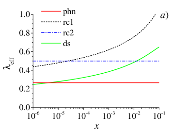
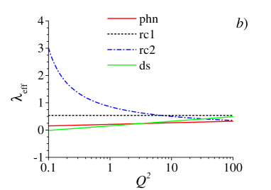
Figure 4: Effective exponents (19) as functions of $x$ for fixed $Q^{2}=10$ GeV²/$c^{2}$ (left) and as functions of $Q^{2}$ for fixed $x=0.0001$ (right).

In order to find the scale relevant for a parameter entering definition of a given scaling variable $\tau$ (4) – (7), for each scaling hypothesis separately we have varied this parameter around the best value by $\pm\epsilon$ and required that

$$|\lambda_{\mathrm{eff}}(\alpha_{\rm min}\pm\epsilon;x,Q^{2})-\lambda_{\mathrm{eff}}(\alpha_{\rm min};x,Q^{2})|=1$$ (20)

for some typical values of $x=0.0001$ and $Q^{2}=10$ GeV${}^{2}/c^{2}$. In this way in each case the value of $\epsilon$ provides the reference scale for each variational parameter $\alpha=\beta,\,\mu,\,\nu$ or $\kappa$. Therefore looking at Fig. 5 one should bear in mind that the span of the vertical axis corresponds to the variation of the effective exponent $\Delta\lambda_{\mathrm{eff}}\sim\pm 1$ around its best value.

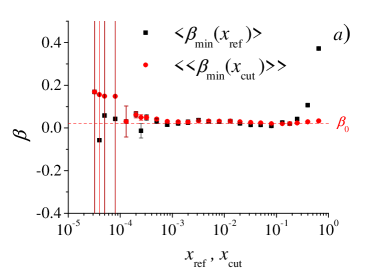
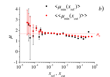
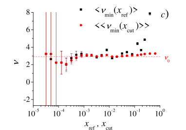
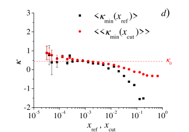
Figure 5: Averaged values $\left\langle\alpha_{\mathrm{min}}(x_{\mathrm{ref}})\right\rangle$ (black squares) and $\left\langle\left\langle\alpha_{\mathrm{min}}(x_{\mathrm{cut}})\right\rangle\right\rangle$ (red circles) for different scaling hypotheses: a) logarithmic $Q^{2}$ effective exponent (4) with $\alpha=\beta$, running coupling scaling variables b) rc1 (5) with $\alpha=\mu$ and d) rc2 (6) with $\alpha=\nu$, and d) diffusive scaling (7) with $\alpha=\kappa$, respectively.

Looking at Figs. 5 we see immediately that the best scaling properties are exhibited by parameter $\beta$ of $Q^{2}$-dependent scaling variable $\tau_{\rm phn}$ (4). Parameter $\beta$ is well described by a constant

$$\beta_{0}=\langle\langle\beta_{\mathrm{min}}(0.08)\rangle\rangle=0.02\pm 0.001$$ (21)

over 3 orders of magnitude in $x$. We have used the value of maximal $x_{\text{cut}}=0.08$, since it was the value of $x_{\text{cut}}$ for which $\lambda_{0}=0.329$ has been extracted in Ref. Praszalowicz:2012zh , although – as clearly seen from Fig. 5.a – GS in variable $\tau_{\rm phn}$ works well up to $x\simeq 0.2$. There is an impressive agreement between both averages $\langle\beta_{\mathrm{min}}\rangle$ and $\langle\langle\beta_{\mathrm{min}}\rangle\rangle,$ however the value (21) is five times smaller than expected from the fit to low $x$ behavior of $F_{2}$ structure function (18).

For comparison in Fig. 6 we present the plot from Ref. Praszalowicz:2012zh where $\langle\lambda_{\mathrm{min}}\rangle$ and $\langle\langle\lambda_{\mathrm{min}}\rangle\rangle$ for scaling hypothesis with constant $\lambda$ (i.e. for $\beta=0$) are shown. We see that the quality of a fit with a constant $\lambda$ is only a little worse than GS in $\tau_{\rm phn}$ but in general much better than in the case of the remaining scaling variables (5) – (7).

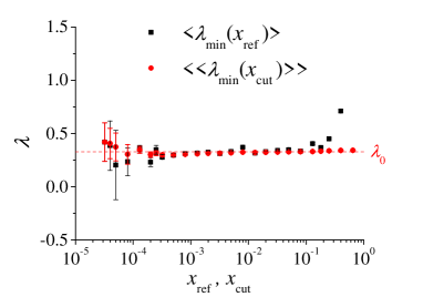
Figure 6: Averaged values $\left\langle\lambda_{\mathrm{min}}(x_{\mathrm{ref}})\right\rangle$ (black squares) and $\left\langle\left\langle\lambda_{\mathrm{min}}(x_{\mathrm{cut}})\right\rangle\right\rangle$ (red circles) for scaling variable with constant exponent $\lambda$ (Eqs. (1) and (3)). Figure from Ref. Praszalowicz:2012zh .

Indeed, for the running coupling constant rc1 case (5) we see in Fig. 5.b monotonous fall of $\langle\mu_{\mathrm{min}}\rangle$ and $\langle\langle\mu_{\mathrm{min}}\rangle\rangle$ with $x_{\text{ref}}$ and $x_{\text{cut}}$ respectively, although the large errors at small $x$’s allow for a constant fit up to $x_{\text{ref}}$, $x_{\text{cut}}\simeq 0.008$ yielding

$$\mu_{0}=\langle\langle\mu_{\mathrm{min}}(0.008)\rangle\rangle=1.677\pm 0.014.$$ (22)

The situation is similar for running coupling rc2 case (6) where the constant fit is possible up to $x_{\text{ref}}$, $x_{\text{cut}}\simeq 0.02$ (see Fig. 5.c) giving

$$\nu_{0}=\langle\langle\nu_{\mathrm{min}}(0.02)\rangle\rangle=2.909\pm 0.025.$$ (23)

In this case, however, one should bear in mind that more ”differential” measure of GS - $\chi^{2}(\nu_{\mathrm{min}})$ - shown in Fig. 3.c does not support hypothesis of GS above $x\sim 10^{-3}$.

Finally, in the case of diffusive scaling (7) we can hardly conclude that GS is really seen; although it is possible to find constant behavior of $\langle\kappa_{\mathrm{min}}\rangle$ and $\langle\langle\kappa_{\mathrm{min}}\rangle\rangle$ below $x\sim 10^{-3}$ with

$$\kappa_{0}=\langle\langle\kappa_{\mathrm{min}}(0.0013)\rangle\rangle=0.449\pm 0.012.$$ (24)

Note, that the errors in Eqs. (21) – (24) are purely statistical (for discussion of systematic uncertainties see Praszalowicz:2012zh ).

4 Summary and Conclusions

In this paper we have applied the method developed in Refs.Stebel:2012ky ; Praszalowicz:2012zh to assess the quality of geometrical scaling of $e^{+}p$ DIS data on $F_{2}$ as provided by the combined H1 and ZEUS analysis of Ref. HERAcombined . In a sense our analysis is in a spirit of previous works Gelis:2006bs ; Beuf:2008bb and especially Ref. Royon:2010tz where the same set of data has been analyzed by means of so called quality factor. Although the authors of Ref. Royon:2010tz applied kinematical cuts $4\leq Q^{2}\leq 150\text{GeV}^{2}$, $x\leq 0.01$ our results for scaling parameters given in Eqs. (16) and (22) – (24) are in good agreement with their findings. For completeness let us quote their results (note that they did not consider logarithmic $Q^{2}$ dependence of $\tau_{\rm phn}$): $\mu_{0}=1.61$ (rc1), $\nu_{0}=2.76$ (rc2) and $\kappa_{0}=0.31$ (ds). Difference in $\kappa_{0}$ can be explained by applied kinematical cuts, indeed, if we take maximal $x_{\rm cut}=0.01$ we obtain $\langle\langle\kappa_{\mathrm{min}}(0.01)\rangle\rangle=0.301\pm 0.006$ in agreement with Royon:2010tz .

Despite the fact that we have been able to find some corners of phase space where geometrical scaling in variables (5) – (7) could be seen, it is absolutely clear that the best scaling variable is given by (4) (or even by a constant $\lambda$ of Eq. (16)), whereas diffusive scaling hypothesis is certainly ruled out. This is quite well illustrated in Fig. 4 where effective exponent $\lambda_{\rm eff}$ for scaling variable (7) changes sign for small $Q^{2}$. This is the reason why in Ref. Royon:2010tz a cut on low $Q^{2}$ has been applied. Similar argument applies for the running coupling rc2 case (6) which blows up for small $Q^{2}$. Because of that $\chi_{x_{i},x_{\text{ref}}}^{2}$ functions have no minima for very low $x_{i}$ and $x_{\text{ref}}$ (points with small $x$ have also small $Q^{2}$). Therefore the only candidate for scaling variable is running coupling rc1 case (5). Nevertheless, comparing Fig. 5.b with Fig. 6 where we plot results for GS scaling with constant exponent $\lambda$, we see that both by quality and applicability range, the original form of scaling variable does much better job than (5). Although our results for best values of parameters entering definitions of scaling variables (5) – (7) are in agreement with Refs. Gelis:2006bs ; Beuf:2008bb ; Royon:2010tz we do not confirm their conclusion that only diffusive scaling is ruled out while for other forms of scaling variable geometrical scaling is of similar quality. It is of course perfectly possible that the HERA data are not ”enough asymptotic” and geometrical scaling in one of the variables defined in Eqs. (5) – (7) will show up at higher energies and lower Bjorken $x$’s.

References

- (1) A.M. Stasto, K.J. Golec-Biernat, J. Kwiecinski, Geometric scaling for the total cross-section in the low x region, Phys. Rev. Lett. 86 (2001) 596 [arXiv:hep-ph/0007192].
-
(2)
K.J. Golec-Biernat, M. Wusthoff,
Saturation effects in deep inelastic scattering at low and its
implications on diffraction, Phys. Rev. D 59 (1998) 014017
[arXiv:hep-ph/9807513];
Saturation in diffractive deep inelastic scattering, Phys. Rev. D 60 (1999) 114023 [arXiv:hep-ph/9903358]. - (3) M. Praszalowicz and T. Stebel, Quantitative Study of Geometrical Scaling in Deep Inelastic Scattering at HERA, [arXiv:1211.5305 [hep-ph]].
- (4) T. Stebel, Master Thesis, Quantitative analysis of Geometrical Scaling in Deep Inelastic Scattering, [arXiv:1210.1567 [hep-ph]].
- (5) A. H. Mueller, Parton Saturation: An Overview, [arXiv:hep-ph/0111244].
- (6) L. McLerran, Strongly Interacting Matter Matter at Very High Energy Density: 3 Lectures in Zakopane, Acta Phys. Pol. B 41 (2010) 2799 [arXiv:1011.3203 [hep-ph]].
-
(7)
J. Jalilian-Marian, A. Kovner, A. Leonidov and H. Weigert,
The BFKL equation from the Wilson renormalization group, Nucl. Phys. B 504 (1997) 415 [arXiv:hep-ph/9701284];
The Wilson renormalization group for low x physics: Towards the high density regime, Phys. Rev. D 59 (1999) 014014 [arXiv:hep-ph/9706377];
E. Iancu, A. Leonidov and L. D. McLerran, Nonlinear gluon evolution in the color glass condensate. 1. Nucl. Phys. A 692 (2001) 583 [hep-ph/0011241];
E. Ferreiro, E. Iancu, A. Leonidov and L. D. McLerran, Nonlinear gluon evolution in the color glass condensate. 2. Nucl. Phys. A 703 (2002) 489 [hep-ph/0109115]. -
(8)
I. Balitsky,
Operator expansion for high-energy scattering,
Nucl. Phys. B 463 (1996) 99
[hep-ph/9509348];
Y. V. Kovchegov, Small x structure function of a nucleus including multiple pomeron exchanges, Phys. Rev. D 60 (1999) 034008 [hep-ph/9901281];
Y. V. Kovchegov, Unitarization of the BFKL pomeron on a nucleus, Phys. Rev. D 61 (2000) 074018 [hep-ph/9905214]. -
(9)
S. Munier and R. B. Peschanski,
Geometric scaling as traveling waves,
Phys. Rev. Lett. 91 (2003) 232001
[hep-ph/0309177];
S. Munier and R. B. Peschanski, Traveling wave fronts and the transition to saturation, Phys. Rev. D 69 (2004) 034008 [hep-ph/0310357]. -
(10)
L. V. Gribov, E. M. Levin and M. G. Ryskin,
Semihard Processes In QCD,
Phys. Rept. 100 (1983) 1;
A. H. Mueller and J-W. Qiu, Gluon recombination and shadowing at small values of x, Nucl. Phys. 268, 427(1986);
A. H. Mueller, Parton Saturation at Small x and in Large Nuclei, Nucl. Phys. B558, 285 (1999) [arXiv:hep-ph/9904404]. -
(11)
L. D. McLerran and R. Venugopalan,
Computing quark and gluon distribution functions for very large nuclei,
Phys. Rev. D 49 (1994) 2233 [arXiv:hep-ph/9309289];
Gluon distribution functions for very large nuclei at small transverse momentum, Phys. Rev. D 49 (1994) 3352 [arXiv:hep-ph/9311205] ;
Green’s functions in the color field of a large nucleus, Phys. Rev. D 50 (1994) 2225 [arXiv:hep-ph/9402335]. -
(12)
V. N. Gribov and L. N. Lipatov,
Deep inelastic e p scattering in perturbation theory,
Sov. J. Nucl. Phys. 15 (1972) 438
(Yad. Fiz. 15 (1972) 781);
G. Altarelli and G. Parisi, Asymptotic Freedom in Parton Language, Nucl. Phys. B 126 (1977) 298;
Y. L. Dokshitzer, Calculation of the Structure Functions for Deep Inelastic Scattering and Annihilation by Perturbation Theory in Quantum Chromodynamics, Sov. Phys. JETP 46 (1977) 641 (Zh. Eksp. Teor. Fiz. 73 (1977) 1216). - (13) J. Kwiecinski and A. M. Stasto, Geometric scaling and QCD evolution, Phys. Rev. D 66, 014013 (2002) and Large geometric scaling and QCD evolution, Acta Phys. Polon. B 33, 3439 (2002).
-
(14)
E.A. Kuraev, L.N. Lipatov, V.S. Fadin,
The Pomeranchuk Singularity in Nonabelian Gauge Theories,
Sov. Phys. JETP 45 (1977) 199
(Zh. Eksp. Teor. Fiz. 72 (1977) 377);
I.I. Balitsky, L.N. Lipatov, The Pomeranchuk Singularity in Quantum Chromodynamics, Sov. J. Nucl. Phys. 28 (1978) 822 (Yad. Fiz. 28 (1978) 1597). - (15) E. Iancu, K. Itakura and L. McLerran, Geometric scaling above the saturation scale, Nucl. Phys. A 708, 327 (2002).
- (16) F. Caola and S. Forte, Geometric Scaling from DGLAP evolution, Phys. Rev. Lett. 101, 022001 (2008).
- (17) J. Bartels, K. J. Golec-Biernat and H. Kowalski, A modification of the saturation model: DGLAP evolution, Phys. Rev. D 66, 014001 (2002) [arXiv:hep-ph/0203258].
- (18) H. Kowalski, L. N. Lipatov, D. A. Ross and G. Watt, Using HERA Data to Determine the Infrared Behaviour of the BFKL Amplitude, Eur. Phys. J. C 70, 983 (2010) [arXiv:1005.0355 [hep-ph]].
- (19) G. Beuf, An Alternative scaling solution for high-energy QCD saturation with running coupling, arXiv:0803.2167 [hep-ph].
-
(20)
E. Iancu, A. H. Mueller and S. Munier,
Universal behavior of QCD amplitudes at high energy from general tools of statistical physics,
Phys. Lett. B 606 (2005) 342
[hep-ph/0410018];
Y. Hatta, E. Iancu, C. Marquet, G. Soyez and D. N. Triantafyllopoulos, Diffusive scaling and the high-energy limit of deep inelastic scattering in QCD at large , Nucl. Phys. A 773 (2006) 95 [hep-ph/0601150]. -
(21)
F. Gelis, R. B. Peschanski, G. Soyez and L. Schoeffel,
Systematics of geometric scaling, Phys. Lett. B 647
(2007) 376 [hep-ph/0610435];
G. Beuf, R. Peschanski, C. Royon and D. Salek, Systematic Analysis of Scaling Properties in Deep Inelastic Scattering, Phys. Rev. D 78 (2008) 074004 [arXiv:0803.2186 [hep-ph]]. - (22) G. Beuf, C. Royon and D. Salek, Geometric Scaling of and in data and QCD Parametrisations, [arXiv:0810.5082 [hep-ph]].
- (23) C. Royon and R. Peschanski, Studies of scaling properties in deep inelastic scattering, PoS DIS 2010 (2010) 282 [arXiv:1008.0261 [hep-ph]].
- (24) F. D. Aaron et al. [H1 and ZEUS Collaboration], Combined Measurement and QCD Analysis of the Inclusive ep Scattering Cross Sections at HERA, JHEP 1001 (2010) 109 [arXiv:0911.0884 [hep-ex]].
- (25) M. Praszalowicz, Violation of Geometrical Scaling in pp Collisions at NA61/SHINE, arXiv:1301.4647 [hep-ph].
-
(26)
L. McLerran, M. Praszalowicz, Saturation and
Scaling of Multiplicity, Mean , Distributions
from 200 GeV 7 TeV, Acta Phys. Pol. B 41
(2010) 1917 [arXiv:1006.4293 [hep-ph]] and
Saturation and Scaling of Multiplicity, Mean , Distributions from 200 GeV 7 TeV – Addendum, Acta Phys. Polon. B 42 (2011) 99 [arXiv:1011.3403 [hep-ph]];
M. Praszalowicz, Improved Geometrical Scaling at the LHC, Phys. Rev. Lett. 106 (2011) 142002 [arXiv:1101.0585 [hep-ph]].