Magnetization and phase transition induced by
circularly polarized laser in quantum magnets

Abstract

We theoretically predict a nonequilibrium phase transition in quantum spin systems induced by a laser, which provides a purely quantum-mechanical way of coherently controlling magnetization. Namely, when a circularly polarized laser is applied to a spin system, the magnetic component of a laser is shown to induce a magnetization normal to the plane of polarization, leading to an ultrafast phase transition. We first demonstrate this phenomenon numerically for an $S=1$ antiferromagnetic Heisenberg spin chain, where a new state emerges with magnetization perpendicular to the polarization plane of the laser in place of the topologically ordered Haldane state. We then elucidate its physical mechanism by mapping the system to an effective static model. The theory also indicates that the phenomenon should occur in general quantum spin systems with a magnetic anisotropy. The required laser frequency is in the terahertz range, with the required intensity being within a prospective experimental feasibility.

I Introduction

There is a growing fascination with physics of nonequilibrium systems, which is becoming an important topic in condensed-matter and other fields of physics. For electron systems, a host of novel phenomena induced in nonequilibrium situations, such as photoinduced Mott transitions Iwai03 ; Okamoto11 ; Aoki14 , photoinduced topological transitions Oka09 ; Wang13 ; Kitagawa11 ; Lindner11 , etc, have been fathomed. Non-equilibrium physics is explored in cold atoms as well, where quantum simulation is being realized Bloch08 ; Simon11 . Now, we pose a question: can we propose novel non-equilibrium phenomena for quantum spin systems as opposed to electron systems? Spin systems are a distinct class of many-body systems, having various possibilities as in recent spintronics, so nonequilibrium phenomena are highly intriguing. Here we propose a novel, nonequilibrium way to coherently control many-body states in spin systems with intense laser fields. In contrast to the control of single quantum states, e.g., qubits, which is becoming important in the field of quantum computation Monroe95 , we want to develop a method to control collective phenomena, such as phase transitions, with a laser.

One way to control electron and atomic systems coherently is to exploit an interaction between matter and laser. Control of spin systems in condensed matter by lasers is becoming a realistic as well as fascinating topic due to recent experimental advances Kampfrath11 ; Kimel05 ; Kirilyuk10 . The key in our study is to use a magnetic component of circularly polarized lasers with photon energy far below the electron energy scale. It was in fact demonstrated recently that a magnetic field of lasers in the terahertz (THz) regime can directly access the spin dynamics without disturbing the charge degrees of freedom of electrons Kampfrath11 . This enables us to focus on coherent spin dynamics since incoherent processes arising from charge excitations can be prevented. While the setup of Ref. Kampfrath11, is within the linear-response regime, here we explore a nonequilibrium avenue in the nonperturbative regime, where we propose that a “laser-induced phase transition” with perfect quantum coherence can be realized. Namely, a circularly polarized laser is shown to induce a net magnetization in quantum antiferromagnets. Most of the previous studies about spin pumping Tserkovnyak02 or spintronics Zutic04 focus on controlling some existing magnetization by a spin torque, which is in sharp contrast with the present nonequilibrium phenomenon where the magnetization rises from zero in a direction perpendicular to the polarization plane of the laser as a purely quantum-mechanical effect.

We first demonstrate the dynamical induction of magnetization numerically with the infinite time-evolving block decimation (iTEBD) Vidal07 ; Barmettler09 for one-dimensional spin chains. The iTEBD is a numerical method that exploits a matrix-product state representation, and can deal with infinite systems (i.e., free of finite size effects) by imposing a spatial periodicity. Through imaginary-time and real-time evolutions, we can obtain the GS and dynamics of a system, respectively.

Dynamical phase transitions require a theoretical treatment that goes beyond the linear-response theory. The Floquet theory is becoming a standard picture for studying quantum systems under time-periodic driving Oka09 ; Kitagawa11 ; Lindner11 ; Tsuji08 . Namely, the time periodicity enables us to cast a time-dependent problem into a static effective model governed by the Floquet Hamiltonian. This has proved to be a useful method in the theory of “Floquet topological insulators” Oka09 ; Kitagawa11 ; Lindner11 , and has also been applied to many-body problems such as a photoinduced Mott transition Tsuji08 . We find here that we can map spin systems in a circularly polarized laser onto static effective systems in a slanted magnetic field using unitary transformation into a rotating frame, or equivalently the Floquet theory. The emergence of the laser-induced magnetization can be understood from this static model, which we confirm by comparing exact diagonalization results with iTEBD. Since the above discussion is also applicable to systems with spatial dimensions higher than one, they should accommodate the induction of magnetization as well.

While the magnetization can be induced in any dimensions, one-dimensional antiferromagnets have, quantum mechanically, a special interest. The system is known to be gapless if the size of each spin $S$ is a half-odd-integer, and gapped if $S$ is an integer. This is the celebrated Haldane’s conjecture Haldane83 , now established by intensive analytic, numerical, and experimental studies. Specifically, the groundstate (GS) of $S=1$ spin chain, known as the Haldane phase, is topologically protected by a symmetry Pollmann10 , and is characterized by a string order parameter Nijs89 . We find an interesting relationship between the size of the induced magnetization and the correlation length of the string order correlation function.

This paper is organized as follows. The setup and the model is described in Sec. II. We explain the mapping from the original model to an effective static one with a rotating frame in Sec. III. Section IV is devoted to an explanation about the relationship between the induced magnetization and the string order correlation function. A summary and discussions, including experimental feasibility, are given in Sec. V.

II Formulation

We consider an application of circularly polarized laser to quantum spin systems, as shown in Fig. 1(a). In this paper, we focus on one-dimensional Heisenberg antiferromagnets with a Hamiltonian,

$${\cal H}_{0}=J\sum_{\langle i,j\rangle}\boldsymbol{S}_{i}\cdot\boldsymbol{S}_{j}+D\sum_{i}(S_{i}^{z})^{2}\quad(J>0),$$ (1)

where the term proportional to the coefficient $D$ is the magnetic anisotropy of a single-ion type. The model is simple, and also known to be realistic for describing, e.g., organic compounds such as ${\rm Ni(C_{2}H_{8}N_{2})_{2}NO_{2}ClO_{4}}$ (NENP) and ${\rm Ni(C_{5}D_{14}N_{2})_{2}N_{3}(PF_{6})}$ (NDMAP). $D/J$ in NENP and NDMAP is estimated from experiments to be about $0.18$ Regnault94 and 0.25 Zheludev01 , respectively. Here, we set $D/J=0.25$.

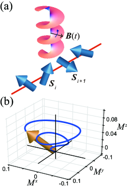
Figure 1: (Color online) (a) A quantum spin system illuminated by a circularly polarized laser is schematically depicted. (b) A typical evolution of the magnetization induced by the laser, which is calculated with iTEBD for $D/J=0.25$, $A/J=1.0$, and $\Omega/J=1.4$. The range of the plot corresponds to about two cycles of the laser (a time interval $0\leq t\leq 9.6J^{-1}$).

We consider a sudden switch-on of the laser at $t=0$ starting from the GS of (1), which is in the Haldane phase Chen03 . The state evolves according to the Hamiltonian

$${\cal H}(t)={\cal H}_{0}-A({\rm e}^{-{\rm i}\Omega t}S^{+}_{\rm tot}+{\rm e}^{{\rm i}\Omega t}S^{-}_{\rm tot})$$ (2)

for $t>0$, where $2A$ and $\Omega$ are the amplitude and frequency (photon energy) of the laser, respectively, and $S_{\rm tot}^{\pm}=S_{\rm tot}^{x}\pm{\rm i}S_{\rm tot}^{y}$ are raising and lowering operators for the total spin ($S_{\rm tot}^{x\;(y,z)}\equiv\sum_{i}S_{i}^{x\;(y,z)}$). Here, we assume that only the magnetic component of the laser couples to the system, and that the laser is applied along the $z$ axis. Thus, each spin feels a magnetic field rotating in the $xy$ plane, $B(S_{\rm tot}^{x}\cos\Omega t+S_{\rm tot}^{y}\sin\Omega t)$, which is expressed above in terms of the spin raising and lowering operators ($B=2A$).

The time evolution of the induced magnetization $\boldsymbol{M}$ ($\equiv\langle\boldsymbol{S}_{i}\rangle$) calculated with iTEBD is displayed in Fig. 1(b). Note that $\boldsymbol{M}$ is normalized so that fully polarized magnetization is 1. The magnetization starts from zero and grows in magnitude with precession. Remarkably, the emerging $\boldsymbol{M}$ tends to point in the $z$ direction, despite the external magnetic field being entirely in the $xy$ plane. There are two conditions for the emergence of magnetization. One is the anisotropy of the spin system. In SU(2) symmetric systems, the spin dynamics becomes trivial since ${\cal H}_{0}$ would then commute with $S^{\pm}_{\rm tot}$ and $S_{\rm tot}^{z}\equiv\sum_{i}S_{i}^{z}$. In the present system, the single-ion magnetic anisotropy, i.e., the $D$ term, lifts this constraint. An Ising-type anisotropy (XXZ model) has a similar effect as well. The second condition is to use a circular polarized light. In a linearly-polarized light, emergence of magnetization perpendicular to the applied magnetic field is prohibited by spin-inversion symmetry.

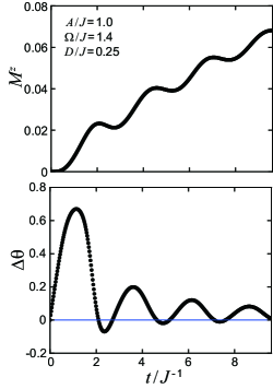
Figure 2: (Color online) Time-evolution of magnetization along $z$-axis $M^{z}$ (top panel), and phase difference, $\Delta\theta$ (bottom), in the $xy$ plane between the laser magnetic field and induced magnetization.

As for a precession of the magnetization, there is an intuitive way to grasp the behavior with a semiclassical spin picture. As can be seen from the numerical result for $M^{z}$ in Fig. 2, the evolution is nonmonotonic. If we compare time evolution of $M^{z}$ with the relative angle between the directions of the external magnetic field and magnetization: $\Delta\theta\equiv\Omega t-\arctan(M^{y}/M^{x})\mod\pi$, the regions for increasing (decreasing) $M^{z}$ are seen to coincide with positive (negative) $\Delta\theta$ regions. This indicates that $\boldsymbol{M}\equiv(M^{x},M^{y},M^{z})$ follows a semi-classical equation, $\dot{\boldsymbol{M}}=\gamma\boldsymbol{M}\times\boldsymbol{B}(t)$, where $\boldsymbol{B}(t)=B(\cos\Omega t,\sin\Omega t,0)$ is the magnetic field of the laser with $\gamma$ a positive constant. If we use fields with opposite circular polarization (left versus right), the magnetization points in the other direction.

However, the emergence of the magnetization is purely a quantum process. In order to clarify the mechanism, we study how the induced magnetization depends on the laser amplitude and frequency. As shown in Fig. 3(a), $M^{z}\propto(A/J)^{2}$ for small $A$. This result indicates that this is a second-order nonlinear process in terms of the laser magnetic field. Figure 3(b) shows the $\Omega$ dependence of $M^{z}$ at various $t$. As time advances, the peak in $M^{z}$ develops around $\Omega/J\simeq 1.4$, which implies a resonance at this frequency. We note that this energy scale is an order of magnitude greater than the Haldane gap $\Delta/J\simeq 0.26$ Golinelli92 , so that this is taken to be a hallmark of the contribution from high-energy excited states. In the following, we explain the induction of magnetization and the resonance behavior in terms of mapping to an effective static model combined with exact diagonalization results.

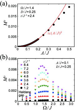
Figure 3: (Color online) (a) $A$ dependence of $M^{z}$ for $t/J^{-1}=2.4$. The solid line is a fit to $M^{z}\propto(A/J)^{2}$. (b) $\Omega$ dependence of $M^{z}$ at various $t$.

III Mapping to a static model

The dynamics of the present system can be understood by mapping it onto a system described by an effective static model using a unitary transformation. The time-dependent Schrödinger equation for the original Hamiltonian (2) is

$$\left[{\rm i}\partial_{t}-{\cal H}(t)\right]|\Psi(t)\rangle=0.$$

If we move on to a reference frame rotating with the magnetic component of laser using a unitary transformation $U=\exp({\rm i}\Omega S_{\rm tot}^{z}t)$, the new state $|\Psi^{\prime}(t)\rangle=U|\Psi(t)\rangle$ satisfies

$$U\left[{\rm i}\partial_{t}-{\cal H}(t)\right]U^{\dagger}|\Psi^{\prime}(t)\rangle=0.$$

With the commutation relations,

$$\big{[}U,{\rm i}\partial_{t}\big{]}U^{\dagger} =\Omega S_{\rm tot}^{z},$$

$$\big{[}U,{\cal H}(t)\big{]}U^{\dagger} =-A\Big{(}{\rm e}^{-{\rm i}\Omega t}[U,S_{\rm tot}^{+}]+{\rm e}^{{\rm i}\Omega t}[U,S_{\rm tot}^{-}]\Big{)}U^{\dagger}$$

$$=-A\left[S_{\rm tot}^{+}(1-{\rm e}^{-{\rm i}\Omega t})+S_{\rm tot}^{-}(1-{\rm e}^{{\rm i}\Omega t})\right]$$

$$=-2AS_{\rm tot}^{x}+A({\rm e}^{-{\rm i}\Omega t}S_{\rm tot}^{+}+{\rm e}^{{\rm i}\Omega t}S_{\rm tot}^{-}),$$

the Schrödinger equation is cast into the form

$$\left[{\rm i}\partial_{t}-\big{(}{\cal H}_{0}-2AS_{\rm tot}^{x}-\Omega S_{\rm tot}^{z}\big{)}\right]|\Psi^{\prime}(t)\rangle=0.$$

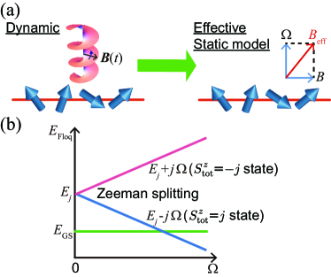
Figure 4: (Color online) (a) The unitary transformation into a rotating frame maps the spin system in circularly polarized laser with amplitude $B$ and frequency $\Omega$ to a static spin model with a slanted magnetic field $\boldsymbol{B}_{\rm eff}=(B,0,\Omega)$. (b) An effective description of the laser-induced magnetization. The magnetic field in the $z$ direction $\Omega$ shifts the many-body energy levels with a “Zeeman splitting.”

Thus we end up with an effective static Hamiltonian

$${\cal H}^{\prime}={\cal H}_{0}-2AS_{\rm tot}^{x}-\Omega S_{\rm tot}^{z},$$ (3)

which is simply a spin system in a slanted magnetic field $\boldsymbol{B}_{\rm eff}=(B,0,\Omega)$ with $B=2A$ [Fig. 4(a)]. We note that this mapping is applicable to arbitrary lattice structures other than the chain considered here. We also note that the effective description has resemblance with the problem of electron spin resonance (e.g., Ref. Oshikawa99, ), where the role of the external magnetic field is here played by the laser frequency $\Omega$. Now the above treatment enables us to understand the mechanism of the laser-induced magnetization process. Excited states with $S_{\rm tot}^{z}=\pm j\;(j>0)$ are initially degenerate due to the spin inversion symmetry ($S_{i}^{z}\to-S_{i}^{z}$). When the laser is turned on, the “longitudinal magnetic field” $\propto\Omega$ lifts the degeneracy due to the Zeeman effect and the energy levels split into $E_{j}\to E_{j}\mp j\Omega$ as shown in Fig. 4(b). The transverse field $B$ acts to hybridize the states having different $S_{\rm tot}^{z}$’s. The hybridization becomes larger as the energies come closer to each other. Since $S_{\rm tot}^{z}=+j$ states approach the GS while $S_{\rm tot}^{z}=-j$ states depart from it, the GS primarily hybridizes with $S_{\rm tot}^{z}=+j$ states, which is precisely why a positive net magnetization appears.

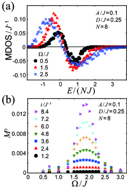
Figure 5: (Color online) (a) Magnetic density of states (MDOS) in units of (number of states)$\cdot J^{-1}$ per site for $\Omega/J$ = 0.5, 1.5, and 2.5. (b) $\Omega$ dependence of $M^{z}$ at various times. The results are obtained by exact diagonalization of the $N=8$ effective Hamiltonian (3).

In the present case, the thermodynamic limit is nontrivial since we have to consider the hybridization with infinitely many levels. To clarify this, let us introduce the “magnetic density of states” (MDOS), defined as $\sum_{i}M_{i}^{z}\delta(E_{i}-E)$, which enables us to capture the behavior of the Zeeman splitting for the entire many-body states. MDOS, normalized by $2^{N}$ ($N$ is the number of spins), for various values of $\Omega$ is calculated with diagonalization of the effective Hamiltonian (3). The result for $A/J=0.1$ and $N=8$ is displayed in Fig. 5(a). While MDOS is zero at $\Omega=0$ due to the $S_{\rm tot}^{z}=\pm j$ degeneracy, it develops positive (negative) peaks on the $E<0$ $(E>0)$ side, which move to low (high) energies with increasing $\Omega$. When the energy of the positive peak overlaps with that of the GS ($E\sim-1.2NJ$), the hybridization becomes most prominent and thus leads to the resonancelike behavior. Figure  5(b) plots $M^{z}$ against $\Omega$ at various times calculated by combining the Floquet theory and the exact diagonalization for $N=8$ (Appendix A). We can see that the result agrees well with the iTEBD result [Fig. 3(b)]. The peak is located around $\Omega/J\simeq 1.9$, which is close to the peak around $\Omega/J\simeq 1.4$ in the iTEBD result. A slight deviation can be attributed to a finite-size effect. We can compare the $\Omega$ dependence of $M^{z}$ at $t/J^{-1}=3.6$ calculated by exact diagonalization for finite size systems $N=4,6,8$ with the iTEBD result for an infinite system in Fig. 6(a). As we increase $N$, the exact diagonalization result approaches that of iTEBD qualitatively. However, a deviation is seen when we use a naive linear extrapolation in the limit of $N\to\infty$ [Fig. 6(b)].

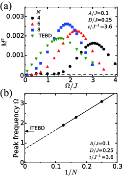
Figure 6: (Color online) (a) $\Omega$ dependence of $M^{z}$ at $t/J^{-1}=3.6$ calculated by exact diagonalization for finite size systems $N=4,6,8$ and by iTEBD for an infinite size system. (b) Peak frequency for $N=4,6,8$, and its linear extrapolation to $N\to\infty$ limit. The arrow represents the peak frequency obtained from iTEBD.

Finally in this section, we note that the emerged magnetization represents not a quantum phase transition but a dynamical phase transition. Due to the sudden onset of the laser (an “ac quench”), the state becomes highly excited. Since the present unitary time evolution described by the static effective model keeps the energy unchanged, the system after the quench does not decay to the GS. Let us display the induced $M^{z}$ for small $A$ and $\Omega$ in Fig. 7. We can see that the induced $M^{z}$ grows as $(A/J)^{2}$, while in the effective model (3) the transition does not occur when the size of the effective field $\sqrt{(2A)^{2}+\Omega^{2}}/J$ is smaller than the Haldane gap $\Delta/J\sim 0.26$. The result implies that the magnetization induction is a dynamical phase transition and not a static quantum phase transition at the absolute zero $T$.

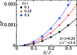
Figure 7: (Color online) The induced $M^{z}$ for small $A$ and $\Omega$. Lines represent fitting of the data points by parabolic curves.

IV Breakdown of the string order

In this section, we present an interesting relation between the induced magnetization and the string order correlation Nijs89 . The Haldane phase, being topologically ordered, has no local order parameter, but is instead characterized by the string order parameter, which is defined as $\lim_{r\to\infty}{\cal O}_{\rm str}(r)$ from the string-order correlation function, ${\cal O}_{\rm str}(r)=\langle S_{0}^{z}\exp({\rm i}\pi\sum_{i=0}^{r-1}S_{i}^{z})S_{r}^{z}\rangle$ Nijs89 . The string order parameter can capture the Haldane phase since this phase consists of a superposition of states in which an arbitrary number of $|S_{i}^{z}=0\rangle$’s are inserted between $|1\rangle$ and $|-1\rangle$ in a Néel order in terms of the $S_{i}^{z}$ basis, e.g., $|\ldots,1,0,0,0,-1,0,1,0,0,-1,\ldots\rangle$. In the initial GS, we are in the Haldane phase with the nonzero string order parameter as seen in the $t=0$ result of Fig. 8(a). For $t>0$, the string order correlation ${\cal O}_{\rm str}(r)$ decays exponentially with distance $r$. This result indicates that the breakdown of the string order happens as soon as the laser application begins.

We find that the decay of the string order has a direct (and even analytic) relation with the emergence of the $z$ component of magnetization. Specifically, the magnetization is related with the string correlation length $\xi$ [defined by fitting ${\cal O}_{\rm str}(r)\propto\exp(-r/\xi)$]. Figure  8(b) plots $\xi^{-1}$ as a function of $M^{z}$. We can deduce an analytic form for the relation between $\xi$ and $M^{z}$ as follows. A flip of a single spin from $|0\rangle$ to $|1\rangle$ or from $|-1\rangle$ to $|0\rangle$ in the Haldane phase gives a factor $-1$ in the string order correlation function, and acts like a “disorder” in the string-ordered states (e.g., $|\ldots,1,0,0,0,-1,0,1,0,0,-1,\ldots\rangle\to|\ldots,1,0,$“1”$,0,-1,0,1,0,0,-1,\ldots\rangle$). The probability of having such a disorder is $M^{z}$ per site, and by estimating the probability of having $k$ disordered sites out of $r$ sites, we are led to an expression,

$${\cal O}_{\rm str}(r) \simeq S_{0}\sum_{k=0}^{r}(-1)^{k}{\,}_{r}{\rm C}_{k}(M^{z})^{k}(1-M^{z})^{r-k}$$

$$=S_{0}(1-2M^{z})^{r},$$

where $S_{0}$ is the initial (i.e., at $M^{z}=0$) value of the string order. Namely, we have $\xi^{-1}=-\ln(1-2M^{z})$, which agrees well with numerical data in Fig. 8(b) in the small $M^{z}$ region.

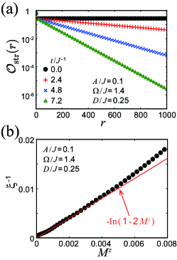
Figure 8: (Color online) (a) The string order correlation function calculated with iTEBD at various times. (b) The inverse of string correlation length $\xi^{-1}$ plotted as a function of $M^{z}$. The result of iTEBD (circles) and the analytical prediction, $\xi^{-1}=-\ln(1-2M^{z})$ (line) are shown.

Now we can comment on the symmetry protection and string order of the Haldane phase. In Ref. Pollmann10, , it is proved that the Haldane phase is characterized by a twofold degeneracy in the entanglement spectrum, and that this degeneracy can be protected by imposing any one of (i) time-reversal, (ii) bond-center inversion, or (iii) $Z_{2}\times Z_{2}$ symmetries. It is also discussed that the string order parameter is well defined in systems with $Z_{2}\times Z_{2}$ symmetry. An example of Haldane phases with no string order is given in Ref. Gu09, . In our case, however, the perturbation is single-ion anisotropy and magnetic field. The single-ion anisotropy, which is unchanged under $S_{i}^{z}\to-S_{i}^{z}$, does not break $Z_{2}\times Z_{2}$ symmetry. This is consistent with our data for $t=0$ in Fig. 8 (a), which shows a nonzero string order parameter. Although the string order parameter cannot be used as an order parameter in the magnetized phase, our finding shows that the decay of the string order correlation function is related with the size of the induced magnetization.

V Summary and discussions

To summarize, we have found that a net magnetization can be induced by applying a circularly polarized laser to antiferromagnets with anisotropy. We numerically demonstrated this phenomenon using iTEBD. The mechanism of the phenomenon and the existence of a resonant frequency are explained by a unitary transformation into a rotating frame, equivalently by the Floquet theory. Then the system is described by an effective static picture, in which the amplitude and frequency of the laser act as transverse and longitudinal magnetic fields, respectively. While the $S=1$ spin chain is initially in the Haldane phase, the laser-induced magnetization occurs concurrently with a destruction of the topological order, which is characterized by an exponential decay of the string order correlation function.

Let us discuss the experimental feasibility. Pump-probe experiments should be most promising, where the pump laser is required to be strong and circularly polarized, and the induced magnetization can be measured by Faraday or Kerr rotation. The necessary pump strength depends on the sensitivity of the probe. We make an estimation for NDMAP, whose exchange interaction is estimated to be $J\simeq 2.8$ meV with $D/J\sim 0.25$ Zheludev01 . While we have considered a continuous laser application, a pulse containing only a few cycles of laser can also induce a magnetization as illustrated in Fig. 1(b). In order to induce $M_{z}\sim 0.01$ with few cycles, we need $A/J\sim 0.1$. This corresponds to $B=2A=0.2J\simeq 5.6$ T. The optimum frequency is, from the resonance frequency, estimated to be $1.4J\simeq 3.9$ meV$\sim 1$ THz. The currently available intensity of the magnetic field in a laser is $\sim 0.13$ T Kampfrath11 , which is still an order of magnitude smaller than the required strength. However, THz laser techniques are rapidly advancing Matsunaga13 ; Hirori11 ; Kirilyuk10 ; Vicario13 , and we expect our theoretical proposal to become experimentally feasible in the near future.

Finally, we comment on the scope of the laser-induced magnetization. While we have presented the result for one-dimensional spin-1 systems, our discussion does not depend on the dimension nor the size of the spin; spin-related phenomena abound in higher dimensions, such as the effect of frustration and emergence of spin liquid phase to name a few. Moreover, quantum spin systems have interdisciplinary spin-offs, e.g., cold-atom systems. It is an interesting future problem to study laser-induced phase transitions in such systems, and the theory presented here is expected to play an important role.

Appendix A Floquet theory

Here let us show that the effective static model (3) can equivalently be obtained using the Floquet theory for many-body systems instead of the unitary transformation onto the rotating frame. The Floquet theory is a mathematical technique to treat time-periodic differential equations, which is a temporal analog of the Bloch theorem for spatially periodic systems. When applied to a time-dependent Schrödinger equation,

$${\rm i}\partial_{t}|\Psi(t)\rangle={\cal H}(t)|\Psi(t)\rangle,$$ (4)

with time periodicity ${\cal H}(t+T)={\cal H}(t)$ ($T$: period), the Floquet theorem dictates that the solution should have a form $|\Psi(t)\rangle={\rm e}^{-{\rm i}\epsilon t}|\Phi(t)\rangle$, which is a product of a phase factor involving $\epsilon$ called Floquet quasi-energy and a time-periodic wave function (Floquet state) with $|\Phi(t+T)\rangle=|\Phi(t)\rangle$. With both ${\cal H}(t)$ and $|\Phi(t)\rangle$ periodic in $t$, we can make a discrete Fourier transform,

$${\cal H}(t) =\sum_{m}{\rm e}^{-{\rm i}m\Omega t}H_{m},$$

$$|\Phi(t)\rangle =\sum_{m}{\rm e}^{-{\rm i}m\Omega t}|\Phi^{m}\rangle.$$

When these are plugged into Eq. (4), the Schrödinger equation is casted into a time-independent eigenvalue equation in a matrix form,

$$\sum_{m}(H_{n-m}-m\Omega\delta_{mn})|\Phi^{m}\rangle=\epsilon|\Phi^{n}\rangle,$$ (5)

which can be thought of as an equation for “photon-dressed” (Floquet) modes.

The present Hamiltonian is a one-dimensional Heisenberg antiferromagnet with a single-ion anisotropy in a circularly polarized field:

$${\cal H}(t)=J\sum_{\langle i,j\rangle}\boldsymbol{S}_{i}\cdot\boldsymbol{S}_{j}+D\sum_{i}(S_{i}^{z})^{2}-A({\rm e}^{-{\rm i}\Omega t}S_{\rm tot}^{+}+{\rm e}^{{\rm i}\Omega t}S_{\rm tot}^{-}).$$ (6)

Thus the zeroth component ($H_{n-m}$ with $n=m$) is $H_{0}=J\sum_{\langle i,j\rangle}\boldsymbol{S}_{i}\cdot\boldsymbol{S}_{j}+D\sum_{i}(S_{i}^{z})^{2}$, and $H_{\pm 1}$ just corresponds to $-AS_{\rm tot}^{\pm}$. The eigenvalue equation (5) then simplifies into a tridiagonal form,

$$\begin{pmatrix}\;\ddots&&&&&&\\ &H_{0}-2\Omega&H_{+1}&0&0&0&\\ &H_{-1}&H_{0}-\Omega&H_{+1}&0&0&\\ &0&H_{-1}&H_{0}&H_{+1}&0&\\ &0&0&H_{-1}&H_{0}+\Omega&H_{+1}&\\ &0&0&0&H_{-1}&H_{0}+2\Omega&\\ &&&&&&\ddots\;\end{pmatrix}\begin{pmatrix}\vdots\\ |\Phi^{2}\rangle\\ |\Phi^{1}\rangle\\ |\Phi^{0}\rangle\\ |\Phi^{-1}\rangle\\ |\Phi^{-2}\rangle\\ \vdots\end{pmatrix}=\epsilon\begin{pmatrix}\vdots\\ |\Phi^{2}\rangle\\ |\Phi^{1}\rangle\\ |\Phi^{0}\rangle\\ |\Phi^{-1}\rangle\\ |\Phi^{-2}\rangle\\ \vdots\end{pmatrix},$$ (7)

where $\Omega$ is a shorthand for $\Omega$ times the unit matrix. The Floquet formalism can then be schematically depicted in Fig. 9(a), where replicas of the original system are prepared for different Floquet (photon-dressed) modes $m$. The terms with the phase factor ${\rm e}^{\mp{\rm i}\Omega t}$ in the Hamiltonian induce a transition from the Floquet mode $m$ to $m\pm 1$.

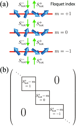
Figure 9: (Color online) (a) Structure of the Floquet Hamiltonian (7) for spin systems in a circularly polarized light field. (b) Block-diagonal structure of the Floquet Hamiltonian reshuffled in terms of the good quantum number $S_{\rm tot}^{z}-m$.

The matrix representation of Eq. (5) is in general infinite-dimensional, since $m$ takes from $-\infty$ to $+\infty$. In the present case, however, $S_{\rm tot}^{z}-m$ is a good quantum number because the term $S_{\rm tot}^{\pm}$ appears in the Hamiltonian with a phase factor ${\rm e}^{\mp{\rm i}\Omega t}$, so that the term simultaneously changes the Floquet index and $S_{\rm tot}^{z}$ by $\pm 1$, respectively, as shown in Fig. 9(a). This implies that the Floquet matrix can be put into a block-diagonal form as shown in Fig. 9(b). We call the Hamiltonian that acts within the blocks an “irreducible Floquet Hamiltonian.” If the system size (i.e., the total number of spins $N$) is finite, each block is finite-dimensional since $S_{\rm tot}^{z}$ is bounded as $-N\leq S_{\rm tot}^{z}\leq N$. Thus, even in the presence of the time-dependent external field, we can readily solve the eigenvalue equation with an exact diagonalization as far as finite systems are concerned. The necessary and sufficient conditions to obtain an irreducible Floquet Hamiltonian are (i) $[H_{0},S_{\rm tot}^{z}]=0$ and (ii) conservation of $S_{\rm tot}^{z}-m$ ($m$: Fourier mode index). These conditions imply that the direction of laser propagation should be parallel to the anisotropy axis of the magnet. This dictates the experimental setup.

The irreducible Floquet Hamiltonian is formally equivalent to the Hamiltonian for an $S=1$ chain with longitudinal and transverse magnetic fields in the present spin model (6). Namely, since the $S_{\rm tot}^{\pm}$ term connects the sectors that have $S_{\rm tot}^{z}$ differing by $\pm 1$, $B(=2A)$ acts as the transverse magnetic field. On the other hand, $\Omega$ acts as the longitudinal magnetic field. We can see this because the matrix components in the same $S_{\rm tot}^{z}$ sector are $H_{0}-m\Omega$, which translates into $H_{0}-\Omega S_{\rm tot}^{z}$ since $S_{\rm tot}^{z}-m$ is constant within each irreducible Floquet Hamiltonian (where the constant, being irrelevant, can be set to 0). We end up with an effective Hamiltonian,

$$H_{\rm Ir.Fl.}=J\sum_{\langle i,j\rangle}\boldsymbol{S}_{i}\cdot\boldsymbol{S}_{j}+D\sum_{i}(S_{i}^{z})^{2}-BS_{\rm tot}^{x}-\Omega S_{\rm tot}^{z}.$$ (8)

The time evolution of $M^{z}$ can then be calculated from the exact diagonalization result for the eigenvalues $\{\epsilon_{\alpha}\}$ and eigenvectors $\{|\Phi_{\alpha}\rangle\}$ of Eq. (8). We can reconstruct the solution of the original time-dependent Schrödinger equation as $|\Psi(t)\rangle=\sum_{\alpha}c_{\alpha}|\Psi_{\alpha}(t)\rangle$, where $|\Psi_{\alpha}(t)\rangle\equiv\sum_{m}{\rm e}^{-{\rm i}(\epsilon_{\alpha}+m\Omega)t}|\Phi_{\alpha}^{m}\rangle$, and the coefficients $c_{\alpha}$, with $\sum_{\alpha}|c_{\alpha}|^{2}=1$ for normalization, is determined from the initial condition. For example, when the application of laser begins suddenly at $t=0$, the coefficients are $c_{\alpha}=\langle\Psi_{\alpha}(t=0)|\Psi_{0}\rangle$, where $|\Psi_{0}\rangle$ is the initial state, i.e., the GS of ${\cal H}_{0}=J\sum_{\langle i,j\rangle}\boldsymbol{S}_{i}\cdot\boldsymbol{S}_{j}+D\sum_{i}(S_{i}^{z})^{2}$. The magnetization per spin $M^{z}$ then evolves as

$$M^{z}(t) =\sum_{\alpha,m}|c_{\alpha}|^{2}\langle\Phi_{\alpha}^{m}|S_{\rm tot}^{z}/N|\Phi_{\alpha}^{m}\rangle$$

$$+\sum_{\alpha<\beta,m}[c_{\beta}^{*}c_{\alpha}{\rm e}^{{\rm i}(\epsilon_{\beta}-\epsilon_{\alpha})t}\langle\Phi_{\beta}^{m}|S_{\rm tot}^{z}/N|\Phi_{\alpha}^{m}\rangle+{\rm H.c.}],$$

where the first (second) term is the $t$-independent ($t$-dependent) part.

Appendix B An animation of the magnetization emergence

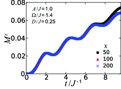
Figure 10: (Color online) The time evolution of $M^{z}$ calculated by iTEBD for the matrix dimension varied as $\chi=50$, 100, 200.

As a best way to represent the time-evolution of the magnetization, we attach here a movie Supplement . There, the initial state ($t=0$) is the GS of

$${\cal H}_{0}=J\sum_{\langle i,j\rangle}\boldsymbol{S}_{i}\cdot\boldsymbol{S}_{j}+D\sum_{i}(S_{i}^{z})^{2}\quad(J>0),$$

and the time evolution for $t>0$ is obtained with iTEBD Vidal07 for the Hamiltonian,

$${\cal H}(t)={\cal H}_{0}-A({\rm e}^{-{\rm i}\Omega t}S_{\rm tot}^{+}+{\rm e}^{{\rm i}\Omega t}S_{\rm tot}^{-}),$$

where we have set $D/J=0.25$, $A/J=1.0$, and $\Omega/J=1.4$. In the movie, the time evolution of magnetization $\boldsymbol{M}=(M^{x},M^{y},M^{z})$ ($M^{\alpha}\equiv\langle S_{i}^{\alpha}\rangle$) is represented by an arrow for a time interval of $0\leq t\leq 9.6J^{-1}$.

Let us mention the precision of iTEBD calculations, which is determined by the dimension $\chi$ of the matrix product state representation. The $\chi$ dependence is shown in Fig. 10. As seen, the $\chi$ dependence is small for $\chi\geq 100$. Thus the calculations for the time interval considered above should be accurate since we have set $\chi=200$ for all iTEBD calculations in our paper.

References

- (1) S. Iwai, M. Ono, A. Maeda, H. Matsuzaki, H. Kishida, H. Okamoto, and Y. Tokura, Phys. Rev. Lett. 91, 057401 (2003).
- (2) H. Okamoto, T. Miyagoe, K. Kobayashi, H. Uemura, H. Nishioka, H. Matsuzaki, A. Sawa, and Y. Tokura, Phys. Rev. B 83, 125102 (2011).
- (3) H. Aoki, N. Tsuji, M. Eckstein, M. Kollar, T. Oka, and P. Werner, Rev. Mod. Phys. 86, 779 (2014).
- (4) Y. H. Wang, H. Steinberg, P. Jarillo-Herrero, and N. Gedik, Science 342, 453 (2013).
- (5) T. Kitagawa, T. Oka, A. Brataas, L. Fu, and E. Demler, Phys. Rev. B 84, 235108 (2011).
- (6) N. H. Lindner, G. Refael, and V. Galitski, Nat. Phys. 7, 490 (2011).
- (7) T. Oka and H. Aoki, Phys. Rev. B 79, 081406(R) (2009); ibid. 79, 169901(E) (2009)”
- (8) I. Bloch, J. Dalibard, and W. Zwerger, Rev. Mod. Phys. 80, 885 (2008).
- (9) J. Simon, W. S. Bakr, R. Ma, M. E. Tai, P. M. Preiss, and M. Greiner, Nature (London) 472, 307 (2011).
- (10) C. Monroe, D. M. Meekhof, B. E. King, W. M. Itano, and D. J. Wineland, Phys. Rev. Lett. 75, 4714 (1995).
- (11) T. Kampfrath, A. Sell, G. Klatt, A. Pashkin, S. Mährlein, T. Dekorsy, M. Wolf, M. Fiebig, A. Leitenstorfer, and R. Huber, Nat. Photon. 5, 31 (2011).
- (12) A. V. Kimel, A. Kirilyuk, P. A. Usachev, R. V. Pisarev, A. M. Balbashov, and Th. Rasing, Nature (London) 435, 655 (2005).
- (13) A. Kirilyuk, A. V. Kimel, and T. Rasing, Rev. Mod. Phys. 82, 2731 (2010).
- (14) Y. Tserkovnyak, A. Brataas, and G. E. W. Bauer, Phys. Rev. B 66, 224403 (2002).
- (15) I. Žutić, J. Fabian, and S. D. Sarma, Rev. Mod. Phys. 76, 323 (2004).
- (16) G. Vidal, Phys. Rev. Lett. 98, 070201 (2007).
- (17) P. Barmettler, M. Punk, V. Gritsev, E. Demler, and E. Altman, Phys. Rev. Lett. 102, 130603 (2009).
- (18) N. Tsuji, T. Oka, and H. Aoki, Phys. Rev. B 78, 235124 (2008).
- (19) F. D. M. Haldane, Phys. Lett. A 93, 464 (1983); Phys. Rev. Lett. 50, 1153 (1983).
- (20) F. Pollmann, A. M. Turner, E. Berg, and M. Oshikawa, Phys. Rev. B 81, 064439 (2010); F. Pollmann, E. Berg, A. M. Turner, and M. Oshikawa, ibid. 85, 075125 (2012).
- (21) M. den Nijs, and K. Rommelse, Phys. Rev. B 40, 4709 (1989).
- (22) L. P. Regnault, I. Zaliznyak, J. P. Renard, and C. Vettier, Phys. Rev. B 50, 9174 (1994).
- (23) A. Zheludev, Y. Chen, C. L. Broholm, Z. Honda, and K. Katsumata, Phys. Rev. B 63, 104410 (2001).
- (24) W. Chen, K. Hida, and B. C. Sanctuary, Phys. Rev. B 67, 104401 (2003).
- (25) O. Golinelli, Th. Jolicoeur, and R. Lacaze, Phys. Rev. B 45, 9798 (1992).
- (26) M. Oshikawa, and I. Affleck, Phys. Rev. Lett. 82, 5136 (1999).
- (27) Z.-C. Gu and X.-G. Wen, Phys. Rev. B 80, 155131 (2009).
- (28) R. Matsunaga, Y. I. Hamada, K. Makise, Y. Uzawa, H. Terai, Z. Wang, and R. Shimano, Phys. Rev. Lett. 111, 057002 (2013).
- (29) H. Hirori, K. Shinokita, M. Shirai, S. Tani, Y. Kadoya, and K. Tanaka, Nat. Commun. 2, 594 (2011).
- (30) C. Vicario, C. Ruchert, F. Ardana-Lamas, P. M. Derlet, B. Tudu, J. Luning, and C. P. Hauri, Nat. Photon. 7, 720 (2013).
- (31) See Supplemental Material at http://link.aps.org/supplemental/10.1103/PhysRevB.90.085150 for an animation movie showing a typical time evolution of the laser-induced magnetization.