Semidefinite approximation for mixed binary quadratically constrained quadratic programs

Abstract

Motivated by applications in wireless communications, this paper develops semidefinite programming (SDP) relaxation techniques for some mixed binary quadratically constrained quadratic programs (MBQCQP) and analyzes their approximation performance. We consider both a minimization and a maximization model of this problem. For the minimization model, the objective is to find a minimum norm vector in $N$-dimensional real or complex Euclidean space, such that $M$ concave quadratic constraints and a cardinality constraint are satisfied with both binary and continuous variables. By employing a special randomized rounding procedure, we show that the ratio between the norm of the optimal solution of the minimization model and its SDP relaxation is upper bounded by $\mathcal{O}(Q^{2}(M-Q+1)+M^{2})$ in the real case and by $\mathcal{O}(M(M-Q+1))$ in the complex case. For the maximization model, the goal is to find a maximum norm vector subject to a set of quadratic constraints and a cardinality constraint with both binary and continuous variables. We show that in this case the approximation ratio is bounded from below by $\mathcal{O}(\epsilon/\ln(M))$ for both the real and the complex cases. Moreover, this ratio is tight up to a constant factor.

1 Introduction

Motivated by applications in wireless communications, we study in this paper two classes of mixed binary nonconvex quadratically constrained quadratic programming (MBQCQP) problems, where the objective functions are quadratic in the continuous variables and the constraints contain continuous and binary variables. Although these two classes of optimization problems are nonconvex, they are amenable to semidefinite programming (SDP) relaxation. The focus of our study is on the approximation bounds of the SDP relaxation for both problems.

The minimization model. Consider the following MBQCQP problem:

$$\min_{\mathbf{w}\in\mathbb{F}^{N},\mbox{\footnotesize\boldmath{$\beta$}}} \quad\|\mathbf{w}\|^{2}$$

$${\rm s.t.} \quad\mathbf{w}^{H}\mathbf{H}_{i}\mathbf{w}\geq\beta_{i}\cdot 1+(1-\beta_{i})\cdot\epsilon,~{}i\in\mathcal{M}$$ (1)

$$\quad\sum_{i\in\mathcal{M}}\beta_{i}\geq Q,$$

$$\quad\beta_{i}\in\{0,1\},~{}i\in\mathcal{M}$$

where $\mathbb{F}$ is either the field of real numbers $\mathbb{R}$ or the field of complex numbers $\mathbb{C}$, $\mathcal{M}=\{1,\cdots,M\}$, ${\mbox{\boldmath$\beta$}}=(\beta_{1},\cdots,\beta_{M})^{T}$, $\mathbf{H}_{i}$ $(i=1,\cdots,M)$ are $N\times N$ real symmetric or complex Hermitian positive semidefinite matrices, $\|\cdot\|$ denotes the Euclidean norm in $\mathbb{F}^{N}$, $M$ and $Q$ are given integers satisfying $1\leq Q\leq M$, and $\epsilon$ is a given parameter satisfying $0\leq\epsilon\leq 1$. Throughout, we use the superscript $H$ to denote the complex Hermitian transpose. Notice that the problem (1) can be easily solved either when $N=1$ or $M=1$, by solving a maximum eigenvalue problem. Hence, we shall assume that $N\geq 2$ and $M\geq 2$ in the rest of the paper. We note that problem (1) is in general NP-hard, due to the fact that one of its special cases with $Q=M$ is NP-hard; see [17, Section 2].

Our interest in problem (1) is motivated by its application in telecommunications. For example, consider a cellular network where $M$ users, each equipped with a single receive antenna, are served by a base station (BS) with $N$ transmit antennas. Assume that a linear transmit beam $\mathbf{w}\in\mathbb{C}^{N\times 1}$ is used by the BS to transmit a common message to the users. Let $\bar{\mathbf{h}}_{i}\in\mathbb{C}^{N\times 1}$ denote the complex channel coefficient between the BS and user $i$, and let $n_{i}$ denote the thermal noise power at the receiver of user $i$. Using these notations, the signal to noise ratio (SNR) at the receiver of each user $i\in\mathcal{M}$ can be expressed as ${\rm SNR}_{i}\triangleq\frac{|\mathbf{w}^{H}\bar{\mathbf{h}}_{i}|^{2}}{n_{i}}$. Such received SNR level measures the quality of the received signal, and is directly related to the effective rate of the communication. In order to successfully decode the transmitted message, typically a quality of service (QoS) requirement in the form of $\frac{|\mathbf{w}^{H}\bar{\mathbf{h}}_{i}|^{2}}{n_{i}}\geq\gamma_{i}$ is imposed by each user $i\in\mathcal{M}$, where $\gamma_{i}$ is a predetermined QoS threshold. Let us define $\mathbf{h}_{i}\triangleq\frac{\bar{\mathbf{h}}_{i}}{\sqrt{n_{i}\gamma_{i}}}$ as user $i$’s normalized channel. When assuming that all $M$ users are served by the BS, the classical physical layer multicast problem can be formulated to the one that minimizes the transmit power of the BS while maintaining the QoS requirements [25]:

$$\min_{\mathbf{w}} \quad\|\mathbf{w}\|^{2}$$ (2)

$${\rm s.t.} \quad{|\mathbf{w}^{H}{\mathbf{h}}_{i}|^{2}}\geq 1,~{}i\in\mathcal{M}.$$

This problem is an NP-hard quadratically constrained quadratic programming (QCQP) problem; see e.g., [25, 17]. It is a continuous homogeneous QCQP problem, which is a special case of the MBQCQP problem (1) when we set $\mathbf{H}_{i}=\mathbf{h}_{i}\mathbf{h}_{i}^{H}$ and $Q=M$.

However, when the number of users in the network is large, it is usually not possible to simultaneously guarantee the QoS for all the users. In this case, user admission control should be implemented to select a subset of users to serve. For instance, we can select to serve a subset of $Q$ users (with $Q$ a given number and $Q\leq M$). This results in the following joint physical layer multicast and admission control problem:

$$\min_{\mathbf{w}\in\mathbb{C}^{N},{\mbox{\boldmath$\beta$}}} \quad\|\mathbf{w}\|^{2}$$ (3)

$${\rm s.t.} \quad{|\mathbf{w}^{H}{\mathbf{h}}_{i}|^{2}}\geq\beta_{i},~{}i\in\mathcal{M}$$

$$\quad\sum_{i\in\mathcal{M}}\beta_{i}\geq Q,\ \ \beta_{i}\in\{0,1\},~{}i\in\mathcal{M}.$$

In the above formulation, the binary variables $\{\beta_{i}\}_{i\in\mathcal{M}}$ indicate whether a particular user $i$ should be served – when $\beta_{i}=0$, there is no guarantee that its QoS constraint will be satisfied. Problem (3) is closely related to a different form of the joint admission control and beamforming problem, in which the goal is to pick the maximum number of users to serve, subject to their respective QoS constraints plus the BS’s power constraint [19, 20, 16]. Obviously, (3) is a special case of the MBQCQP problem (1) if we set $\mathbf{H}_{i}=\mathbf{h}_{i}\mathbf{h}_{i}^{H}$, for all $i\in\mathcal{M}$ and $\epsilon=0$.

An effective approach to approximately solve the NP-hard problem (2) is to use the semidefinite programming relaxation technique [18] together with a randomized rounding step. The idea is to first reformulate the problem by introducing a rank-1 matrix $\mathbf{X}=\mathbf{w}\mathbf{w}^{H}$. After dropping the nonconvex rank-1 constraint on $\mathbf{X}$, the relaxed problem becomes an SDP, whose optimal solution ${\bar{\mathbf{X}}}$ can be efficiently computed. A randomization procedure then follows which converts ${\bar{\mathbf{X}}}$ to a feasible solution of (2). It has been shown in [17] that such SDP relaxation scheme generates high-quality solutions, whose worst case performance bound can be explicitly characterized. Notice that if $\epsilon=1$ or $Q=M$, then problem (1) reduces to a continuous homogeneous QCQP problem for which the theoretical ratio between its optimal solution and the SDP relaxation has been shown to be upper bounded by $27M^{2}/\pi$ [17]. However, for the general case when $0\leq\epsilon<1$ with both binary and continuous variables, there is no known performance guarantees for the performance of SDP relaxation techniques.

The maximization model. Another interesting case of the MBQCQP problem takes the maximization form as follows:

$$\max_{\mathbf{w}\in\mathbb{F}^{n},{\mbox{\boldmath$\beta$}}} \quad\|\mathbf{w}\|^{2}$$

$${\rm s.t.} \quad\mathbf{w}^{H}\mathbf{H}_{i}\mathbf{w}\leq\beta_{i}\cdot\epsilon+(1-\beta_{i})\cdot 1,~{}i\in\mathcal{M}$$ (4)

$$\quad\sum_{i\in\mathcal{M}}\beta_{i}\geq Q,\ \ \beta_{i}\in\{0,1\},~{}i\in\mathcal{M}$$

where $0\leq\epsilon\leq 1$ and $1\leq Q\leq M$. The above MBQCQP problem (4) arises naturally in the interference suppression problem in radar or wireless communication. Here, the interference suppression is captured by the constraints (4), in which the constants $\epsilon$ and $1$ represent two distinctive suppression levels. The optimization problem becomes the one that maximizes the gain of the antenna array while suppressive undesirable interferences. Notice that problem (4) can be easily solved when $N=1$ or $M=1$. As a result we assume $N\geq 2$ and $M\geq 2$ in the rest of the paper.

Notice that if $\epsilon=1$, then problem (4) reduces to a continuous homogeneous QCQP problem for which the theoretical ratio between its optimal solution and the SDP relaxation has been shown to be bounded below by $\mathcal{O}(1/\ln(M))$ [2, 17, 31]. However, for the general case when $0\leq\epsilon<1$, no approximation bounds for SDP relaxation are known.

Our Contributions. In Sections $2$ and $3$, we develop two types of SDP relaxations for the optimization models (3) and (4): One applies SDP relaxation to both the binary and the continuous variables, while the other way simply relaxes binary variables to continuous variables and uses the SDP relaxation for the other continuous variables. Interestingly, we prove that these two types of SDPs are equivalent. Given an optimal solution of the relaxed problem, we devise a novel randomization procedure to generate approximate solutions for the original NP-hard MBQCQP problems. Moreover, we analyze the quality of such approximate solutions by deriving bounds on the approximation ratios between the optimal solution of the two MBQCQP problems and those of their corresponding SDP relaxations. Our main results are as follows: i) For the problem (P1), when $\epsilon=0$, the approximation ratio is upper bounded by $\mathcal{O}(Q^{2}(M-Q+1))$ for the real case and by $\mathcal{O}(Q(M-Q+1))$ for the complex case; when $0<\epsilon<1$, the approximation ratio is upper bounded by $\mathcal{O}(Q^{2}(M-Q+1)+M^{2})$ for the real case and by $\mathcal{O}(M(M-Q+1))$ for the complex case; ii) For the problem (4), the ratio can be arbitrarily bad when $\epsilon=0$; otherwise it is bounded from below by $\mathcal{O}(\epsilon/\ln(M))$ for both the real and the complex cases. To the best of knowledge, our analysis is the first attempt to rigorously characterize the approximation bounds for MBQCQP-type problems and their SDP relaxations.

Related Literature. There is a sizeable literature on the quality bounds of SDP relaxation for solving nonconvex QCQP problems, including the works of Luo et al. [17], Nemirovski et al. [21], A. Ben-Tal et al. [2]. Moreover, for the max-cut problem, which is a special QCQP problem with only discrete variables, Goemans and Williamson [9] showed that the ratio of the optimal value of SDP relaxation over that of the original problem is bounded below by $0.87856\ldots$. For closely related results, see [30, 8]. Moreover, there may not be any meaningful worst-case approximation ratio between certain discrete quadratic optimization problems and their semidefinite relaxation (see, e.g., Proposition 3.1 in [27] or the discussion in [14]). In the absence of the discrete constraints, Beck and Teboulle [1] considered the continuous nonconvex problem of minimizing the ratio of two nonconvex quadratic functions over a possibly degenerate ellipsoid, and showed that the SDP relaxation can return exact solutions under a certain condition. He et al. [11] showed that the ratio between the optimal value of a homogeneous continuous QCQP problem and its the SDP relaxation is upper bounded by $\mathcal{O}(M^{2})$ (resp. $\mathcal{O}(M)$) in the real (resp. complex) case, if all but one of the quadratic constraints are convex. However, for the mixed binary and continuous type QCQP problems, there is no known approximation bounds for SDP relaxations.

Another popular method to approximately solve the MBQCQP problem is to relax the 0-1 variables to continuous variables in the interval $[0,1]$. However, this approach is effective only when the resulting continuous relaxation problem is itself convex. Under this assumption, a variety of algorithms have been proposed, including branch and bound [28], outer approximation [7], the extended cutting-plane method [29], and so on. Unfortunately, for the two optimization models (P1) and (4) considered in this paper, their continuous relaxations are nonconvex. In this case, there is no known approximation quality analysis results. However, surprisingly, we will show that for our two models, to do the continuous relaxation and the SDP relaxation for the discrete variables are equivalent. Moreover, we obtain some approximation bounds for the SDP relaxation. In a recent paper, Billionnet et al. [4] proposed a method called Quadratic Convex Reformulation (QCR) to convert nonconvex 0-1 QP problems to convex ones by using SDP, rather than merely relax them. In their follow-up paper, Billionnet et al. [3] extended the QCR framework from 0-1 QP to mixed-integer quadratic programming (MIQP). However, their approach works only under certain restrictive assumptions, e.g., the objective and the constraints corresponding to the continuous variables are convex, which unfortunately do not hold in our current context. Some alternative approaches to MBQCQP have recently appeared in [5, 23, 24]. More detailed reviews of recent progress on related problems can be found in the excellent surveys [6, 12, 15].

Notations. For a symmetric matrix $\mathbf{X}$, $\mathbf{X}\succeq 0$ signifies that $\mathbf{X}$ is positive semi-definite. We use ${\mbox{{Tr}}}\left[\mathbf{X}\right]$ and $\mathbf{X}[i,j]$ to denote the trace and the $(i,j)$th element of a matrix $\mathbf{X}$, respectively. For a vector $\mathbf{x}$, we use $\|\mathbf{x}\|$ to denote its Euclidean norm, and use $\mathbf{x}[i]$ to denote its $i$th element. For a real vector $\mathbf{y}$, use $\mathbf{y}_{[m]}$ to denote its $m$th largest elements. For a complex scalar $x$, its complex conjugate is denoted by $\bar{x}$. The notation $\mathbf{I}_{n}$ is used to denote a $n\times n$ identity matrix. Given a set $\mathcal{A}$, $|\mathcal{A}|$ denotes the number of elements in set $\mathcal{A}$. Also, we use $\mathbb{R}^{N\times M}$ and $\mathbb{C}^{N\times M}$ to denote the set of real and complex $N\times M$ matrices, and use $\mathbb{S}^{N}$ and $\mathbb{S}^{N}_{+}$ to denote the set of $N\times N$ hermitian and hermitian positive semi-definite matrices, respectively. We use ${\mathbb{E}}(\cdot)$ to denote the expectation operator. Let $\mathbf{e}_{i}$ denote the $i$th unit vector whose entries are all zero except $\mathbf{e}_{i}[i]=1$, and let $\mathbf{e}$ denote the all $1$ vector. Finally, we use the superscript $H$ and $T$ to denote the complex Hermitian transpose and transpose of a matrix or a vector respectively.

2 Approximation bounds for the minimization model

2.1 Reformulation and two SDP relaxations

In this section we consider the minimization problem (1) and its SDP relaxation.

We first consider the SDP relaxation for both the discrete and the continuous constraints. Notice that, by monotonicity, we can assume without loss of generality that the inequality constraint $\sum_{i\in\mathcal{M}}\beta_{i}\geq Q$ in (1) holds with equality, resulting in the following equivalent formulation:

$$\min_{\mathbf{w}\in\mathbb{F}^{N},\mbox{\footnotesize\boldmath$\beta$}} \quad\|\mathbf{w}\|^{2}$$

$${\rm s.t.} \quad\mathbf{w}^{H}\mathbf{H}_{i}\mathbf{w}\geq\beta_{i}\cdot 1+(1-\beta_{i})\cdot\epsilon,~{}i\in\mathcal{M}$$ (P1)

$$\quad\sum_{i\in\mathcal{M}}\beta_{i}=Q,\ \ \beta_{i}\in\{0,1\},~{}i\in\mathcal{M}$$

By performing a simple transformation $\alpha_{i}=2\beta_{i}-1$, for all $i\in\mathcal{M}$, we convert the range of the binary variables to $\{-1,1\}$. We further introduce an auxiliary binary variable $\ell\in\{-1,1\}$, and transform the problem (P1) equivalently to

$$\min_{\mathbf{w}\in\mathbb{F}^{N},(\mbox{\footnotesize\boldmath$\alpha$},\ell)} \quad\|\mathbf{w}\|^{2}$$

$${{\rm s.t.}} \quad\mathbf{w}^{H}\mathbf{H}_{i}\mathbf{w}+\frac{1}{4}(\alpha_{i}-(1-\epsilon)\ell)^{2}\geq 1+\frac{\epsilon^{2}}{4},\ i\in\mathcal{M}$$

$$\quad\sum_{i=1}^{M}(\alpha_{i}+\ell)^{2}=4Q$$

$$\quad\ell^{2}=1,\ \alpha^{2}_{i}=1,\ \ i\in\mathcal{M}.$$

To write the above problem in a more compact form, we make the following definitions:

$$\mathbf{C}_{i} \triangleq\frac{1}{4}\mathbf{e}_{i}\mathbf{e}^{T}_{i}+\frac{(1-\epsilon)^{2}}{4}\mathbf{e}_{M+1}\mathbf{e}^{T}_{M+1}-\frac{1-\epsilon}{4}\mathbf{e}_{i}\mathbf{e}^{T}_{M+1}-\frac{1-\epsilon}{4}\mathbf{e}_{M+1}\mathbf{e}^{T}_{i}\in\mathbb{R}^{(M+1)\times(M+1)}$$

$$\mathbf{A}_{i} \triangleq\left[\begin{array}[]{ll}\mathbf{C}_{i}&\bf{0}\\ \bf{0}&\mathbf{H}_{i}\end{array}\right]\in\mathbb{F}^{(M+1+N)\times(M+1+N)},\ \ \mathbf{B}\triangleq\left[\begin{array}[]{lll}\mathbf{I}&\mathbf{e}&\bf{0}\\ \mathbf{e}^{T}&M&\bf{0}\\ \bf{0}&\bf{0}&\bf{0}\end{array}\right]\in\mathbb{R}^{(M+1+N)\times(M+1+N)}$$ (10)

$$\mathbf{x}^{(1)} \triangleq[{\mbox{\boldmath$\alpha$}}^{T},\ell]^{T},\ \mathbf{x}^{(2)}\triangleq\mathbf{w},\ \mathbf{x}\triangleq[\mathbf{x}^{(1)T},\mathbf{x}^{(2)T}]^{T}.$$

With these definitions, the problem can be written as the following homogeneous QCQP problem:

$$v^{\min}_{{\rm QP}}\triangleq\min_{\mathbf{x}} \quad\|\mathbf{x}^{(2)}\|^{2}$$

$${{\rm s.t.}} \quad\mathbf{x}^{H}\mathbf{A}_{i}\mathbf{x}\geq 1+\frac{\epsilon^{2}}{4},\ i\in\mathcal{M}$$ (11)

$$\quad\mathbf{x}^{H}\mathbf{B}\mathbf{x}=4Q,$$

$$\quad(\mathbf{x}[i])^{2}=1,\ i\in\mathcal{M}.$$

Let ${\bar{\mathbf{x}}}$ be a global optimal solution of problem (11), and $v^{\min}_{{\rm QP}}$ be the optimal objective value.

To obtain an approximate solution for the nonconvex quadratic problem (11), let us consider its SDP relaxation. However, caution should be exercised when relaxing (11)—unlike the conventional QCQP problem studied in, e.g., [18, 17], the nonconvexity of our current problem arises from both continuous and binary variables. To proceed, let us introduce a new matrix variable $\mathbf{X}\triangleq\mathbf{x}\mathbf{x}^{H}$, which admits the following block structure

$$\mathbf{X} =\left[\begin{array}[]{ll}\mathbf{X}^{(1)}&\mathbf{X}^{(3)}\\ (\mathbf{X}^{(3)})^{H}&\mathbf{X}^{(2)}\end{array}\right]\in\mathbb{S}^{(M+1+N)\times(M+1+N)}_{+}$$ (14)

where $\mathbf{X}^{(1)}\triangleq\mathbf{x}^{(1)}(\mathbf{x}^{(1)})^{H}$, $\mathbf{X}^{(2)}\triangleq\mathbf{x}^{(2)}(\mathbf{x}^{(2)})^{H}$, $\mathbf{X}^{(3)}\triangleq\mathbf{x}^{(1)}(\mathbf{x}^{(2)})^{H}$, and the ranks of matrices $\mathbf{X}^{(1)}$, $\mathbf{X}^{(2)}$ and $\mathbf{X}$ are all $1$. By dropping all the rank-1 constraints, we obtain the following SDP relaxation problem for (11):

$$\min \quad{\mbox{{Tr}}}[\mathbf{X}^{(2)}]$$

$${{\rm s.t.}} \quad{\mbox{{Tr}}}[\mathbf{A}_{i}\mathbf{X}]\geq 1+\frac{\epsilon^{2}}{4},\ i\in\mathcal{M}$$ (15)

$$\quad{\mbox{{Tr}}}[\mathbf{B}\mathbf{X}]=4Q,$$

$$\quad\mathbf{X}^{(1)}[i,i]=1,\quad i\in\mathcal{M},\quad\mathbf{X}\succeq 0.$$

Let ${\tilde{\mathbf{X}}}$ denote the optimal solution for this problem, from the block diagonal structure of the matrices $\mathbf{C}_{i},\mathbf{A}_{i},\mathbf{B}$, it is easy to see that ${\tilde{\mathbf{X}}}^{(1)}$ is a real symmetric PSD matrix, and that without loss of generality we can assume ${\tilde{\mathbf{X}}}^{(3)}={\bf 0}$. Moreover, under this assumption, problem (15) can be equivalently reformulated as:

$$v^{\min}_{{\rm SDP1}}\triangleq\min \quad{\mbox{{Tr}}}[\mathbf{X}^{(2)}]$$

$${{\rm s.t.}} \quad{\mbox{{Tr}}}\left[\mathbf{H}_{i}{\mathbf{X}}^{(2)}\right]\geq\left[\frac{1+\mathbf{X}^{(1)}[i,M+1]}{2}\right]+\left[\frac{1-\mathbf{X}^{(1)}[i,M+1]}{2}\right]\cdot\epsilon,\ i\in\mathcal{M}$$ (SDP1)

$$\quad\sum_{i\in\mathcal{M}}\mathbf{X}^{(1)}[i,M+1]=2Q-M,$$

$$\quad\mathbf{X}^{(1)}[i,i]=1,\ i\in\mathcal{M},\quad\mathbf{X}^{(1)}\succeq 0,\ \mathbf{X}^{(2)}\succeq 0,$$

where the variables are $\mathbf{X}^{(1)}$ and $\mathbf{X}^{(2)}$, corresponding to the SDP relaxation matrices for the discrete variables and the continuous variables respectively. Let ${\tilde{\mathbf{X}}^{(1)}}$ and ${\tilde{\mathbf{X}}^{(2)}}$ denote the optimal solution for this problem, and let $v^{\min}_{{\rm SDP1}}$ denote its optimal objective value.

Alternatively, by relaxing the binary variables to continuous variables in the interval $[0,1]$, while still using SDP relaxation for the continuous variables, we can derive another SDP relaxation problem for (P1):

$$v^{\min}_{{\rm SDP2}}\triangleq\min \quad{\mbox{{Tr}}}[\mathbf{X}^{(2)}]$$

$${{\rm s.t.}} \quad{\mbox{{Tr}}}\left[\mathbf{H}_{i}{\mathbf{X}}^{(2)}\right]\geq\beta_{i}\cdot 1+(1-\beta_{i})\cdot\epsilon,\ i\in\mathcal{M}$$ (SDP2)

$$\quad\sum_{i\in\mathcal{M}}\beta_{i}=Q,\quad 0\leq\beta_{i}\leq 1,\ i\in\mathcal{M}$$

$$\quad\mathbf{X}^{(2)}\succeq 0.$$

Let $\bar{\mbox{\boldmath$\beta$}}=(\bar{\beta}_{1},\cdots,\bar{\beta}_{M})^{T}$ and $\bar{\mathbf{X}}^{(2)}$ denote the optimal solution for this problem, and let $v^{\min}_{{\rm SDP2}}$ denote its optimal objective value. As is well known, SDP relaxation usually yields tighter bounds than the continuous relaxation in many cases. However, as shown in the following lemma, the two SDP relaxations (SDP1) and (SDP2) for the problem (P1) are equivalent.

Lemma 1.

Let $(\tilde{\mathbf{X}}^{(1)},\tilde{\mathbf{X}}^{(2)})$ be an optimal solution of the problem (SDP1), then $(\tilde{{\mbox{\boldmath$\beta$}}},\tilde{\mathbf{X}}^{(2)})$ is an optimal solution for (SDP2), with $\tilde{{\mbox{\boldmath$\beta$}}}[i]=\frac{1}{2}+\frac{1}{2}\tilde{\mathbf{X}}^{(1)}[i,M+1]$, $\forall\;i\in\mathcal{M}$. The converse is also true.

Proof.

Let ${\mbox{\boldmath$\gamma$}}=(\gamma_{1},\cdots,\gamma_{M})^{T}$ with $\gamma_{i}=\frac{1}{2}+\frac{1}{2}\mathbf{X}^{(1)}[i,M+1]$ ($i\in\mathcal{M}$) and $\mathbf{a}=(\mathbf{X}^{(1)}[1,M+1],\cdots,\mathbf{X}^{(1)}[M,M+1])^{T}$, then we have $\mathbf{a}=2{\mbox{\boldmath$\gamma$}}-\mathbf{e}$ and $\mathbf{X}^{(1)}$ can be written as

$$\mathbf{X}^{(1)} =\left[\begin{array}[]{ll}\mathbf{Y}&\mathbf{a}\\ \mathbf{a}^{T}&1\end{array}\right],$$ (18)

where $\mathbf{Y}\in\mathbb{S}^{M\times M}$. By Schur Complement, we know that $\mathbf{X}^{(1)}\succeq 0$ is equivalent to $\mathbf{Y}\succeq\mathbf{a}\mathbf{a}^{T}=(2{\mbox{\boldmath$\gamma$}}-\mathbf{e})(2{\mbox{\boldmath$\gamma$}}-\mathbf{e})^{T}$. With these definitions and observations, it can be concluded that (SDP1) is equivalent to the following problem:

$$\min \quad{\mbox{{Tr}}}[\mathbf{X}^{(2)}]$$

$${{\rm s.t.}} \quad{\mbox{{Tr}}}\left[\mathbf{H}_{i}{\mathbf{X}}^{(2)}\right]\geq\gamma_{i}+(1-\gamma_{i})\cdot\epsilon,\ i\in\mathcal{M}$$ (19)

$$\quad\sum_{i\in\mathcal{M}}\gamma_{i}=Q,$$

$$\quad\mathbf{Y}[i,i]=1,i\in\mathcal{M},\quad\mathbf{Y}\succeq(2{\mbox{\boldmath$\gamma$}}-\mathbf{e})(2{\mbox{\boldmath$\gamma$}}-\mathbf{e})^{T},\mathbf{X}^{(2)}\succeq 0.$$

Assume $(\tilde{\mathbf{X}}^{(1)},\tilde{\mathbf{X}}^{(2)})$ is an optimal solution for the problem (SDP1) with

$$\tilde{\mathbf{X}}^{(1)} =\left[\begin{array}[]{ll}\tilde{\mathbf{Y}}&2\tilde{\mbox{\boldmath$\beta$}}-\mathbf{e}\\ (2\tilde{\mbox{\boldmath$\beta$}}-\mathbf{e})^{T}&1\end{array}\right],$$ (22)

with $\tilde{\mbox{\boldmath$\beta$}}=\frac{1}{2}+\frac{1}{2}\tilde{\mathbf{X}}^{(1)}[i,M+1]$ ($i\in\mathcal{M}$), then $(\tilde{\mathbf{Y}},\tilde{\mbox{\boldmath$\beta$}},\tilde{\mathbf{X}}^{(2)})$ will be an optimal solution for (19). By $\tilde{\mathbf{Y}}[i,i]=1,i\in\mathcal{M}$ and $\tilde{\mathbf{Y}}\succeq(2\tilde{\mbox{\boldmath$\beta$}}-\mathbf{e})(2\tilde{\mbox{\boldmath$\beta$}}-\mathbf{e})^{T}$, we have

$$-\mathbf{e}\leq 2\tilde{\mbox{\boldmath$\beta$}}-\mathbf{e}\leq\mathbf{e},$$

or equivalently $0\leq\tilde{\mbox{\boldmath$\beta$}}_{i}\leq 1$, $i\in\mathcal{M}$. It follows that $(\tilde{\mbox{\boldmath$\beta$}},\tilde{\mathbf{X}}^{(2)})$ is a feasible solution of (SDP2). Thus, if $(\bar{{\mbox{\boldmath$\beta$}}},\bar{\mathbf{X}}^{(2)})$ is an optimal solution of (SDP2), then

$${\mbox{{Tr}}}[\tilde{\mathbf{X}}^{(2)}]\geq{\mbox{{Tr}}}[\bar{\mathbf{X}}^{(2)}].$$ (23)

Moreover, by the feasibility of $\bar{{\mbox{\boldmath$\beta$}}}$, we have

$$-\mathbf{e}\leq 2\bar{{\mbox{\boldmath$\beta$}}}-\mathbf{e}\leq\mathbf{e}.$$ (24)

Denote $\Delta\in\mathbb{S}_{+}^{M}$ as a diagonal matrix with its $i$-th diagonal element given by $1-(2\bar{\mbox{\boldmath$\beta$}}[i]-1)^{2}\geq 0$ , for all $i\in\mathcal{M}$. Using this definition, we further define a matrix $\tilde{\mathbf{Y}}$ by

$$\tilde{\mathbf{Y}}=(2\bar{{\mbox{\boldmath$\beta$}}}-\mathbf{e})(2\bar{{\mbox{\boldmath$\beta$}}}-\mathbf{e})^{T}+\Delta.$$ (25)

Then, it can be easily checked that $(\tilde{\mathbf{Y}},\bar{\mathbf{X}}^{(2)},\bar{{\mbox{\boldmath$\beta$}}})$ is a feasible solution for (19), and

$${\mbox{{Tr}}}[\bar{\mathbf{X}}^{(2)}]\geq{\mbox{{Tr}}}[\tilde{\mathbf{X}}^{(2)}].$$ (26)

By combining(23) and (26), we have that ${\mbox{{Tr}}}[\bar{\mathbf{X}}^{(2)}]={\mbox{{Tr}}}[\tilde{\mathbf{X}}^{(2)}]$. Moveover, it can also be concluded that $(\tilde{\mbox{\boldmath$\beta$}},\tilde{\mathbf{X}}^{(2)})$ is an optimal solution for (SDP2).

The proof of the reverse part is similar and is omitted for space reason. ∎

By Lemma 1, we have $v^{\min}_{{\rm SDP1}}=v^{\min}_{{\rm SDP2}}\leq v^{\min}_{{\rm QP}}$. Due to its smaller problem size, the SDP relaxation problem (SDP2) is preferred.

Remark: As suggested by an anonymous referee, we can use slightly different technique to derive another SDP relaxation for (P1). Specifically, we first consider the following continuous relaxation of (P1):

$$\min \quad\|\mathbf{w}\|^{2}$$

$${\rm s.t.} \quad\mathbf{w}^{H}\mathbf{H}_{i}\mathbf{w}\geq\alpha_{i},~{}i=1,\cdots,M$$ (27)

$$\quad\sum_{i=1}^{m}\min\{1,\alpha_{i}\}=Q+(M-Q)\cdot\epsilon,$$

$$\quad\alpha_{i}\geq\epsilon,~{}i=1,\cdots,M.$$

This is a relaxation because any feasible solution $(\mathbf{w},{\mbox{\boldmath$\beta$}})$ to the problem (P1) is feasible to problem (27) by letting ${\mbox{\boldmath$\alpha$}}={\mbox{\boldmath$\beta$}}+\epsilon(\mathbf{e}-{\mbox{\boldmath$\beta$}})$. Then, we consider an SDP relaxation to the above continuous problem

$$\min \quad{\mbox{{Tr}}}{(\mathbf{X})}$$

$${\rm s.t.} \quad{\mbox{{Tr}}}{(\mathbf{H}_{i}\mathbf{X})}\geq\alpha_{i},~{}i=1,\cdots,M,$$ (28)

$$\quad\sum_{i=1}^{m}\min\{1,\alpha_{i}\}=Q+(M-Q)\epsilon,$$

$$\quad\alpha_{i}\geq\epsilon,~{}i=1,\cdots,M,$$

$$\quad\mathbf{X}\succeq 0.$$

Although (28) and (SDP2) are derived differently, they are equivalent in the sense that they have the same optimal solution matrix and hence the same optimal objective value. This can be verified easily (we omit the details here). It is also important to note that the two SDP problems have the same problem size and the same number of variables. In the rest of the paper we will use (SDP2) as the basis for our analysis.

In the following, we aim to generate a feasible solution $\mathbf{x}$ for (P1) from ${(\bar{\mbox{\boldmath$\beta$}},\bar{\mathbf{X}}^{(2)})}$, and evaluate the quality of such solution. In particular, we would like to find a constant $\mu\geq 1$ such that

$$\|\mathbf{x}^{(2)}\|^{2}\leq\mu v^{\min}_{{\rm SDP2}}.$$

By using the fact that such generated solution is feasible for problem (P1), we have $v^{\min}_{{\rm QP}}\leq\|\mathbf{x}^{(2)}\|^{2}$, which further implies that the same $\mu$ is an upper bound of the SDP relaxation performance, i.e.,

$$v^{\min}_{{\rm QP}}\leq\mu v^{\min}_{{\rm SDP2}}.$$ (29)

The constant $\mu$ will be referred to as the approximation ratio.

2.2 A new randomization procedure

Upon obtaining the optimal solution ${(\bar{\mbox{\boldmath$\beta$}},\bar{\mathbf{X}}^{(2)})}$ of problem (SDP2), we propose to use the randomization procedure outlined in Table 1 to obtain a feasible solution for problem (P1). In essence, this procedure consists of the following two parts.

Part 1) This includes Steps S1 and S2 in Table 1, in which we generate the binary variable $\mathbf{x}^{(1)}$ from ${\bar{\mbox{\boldmath$\beta$}}}$. It is easy to verify that $\mathbf{x}^{(1)}$ generated in this way satisfies the constraints $\sum_{i\in\mathcal{M}}\mathbf{x}^{(1)}_{i}=Q$ and $\mathbf{x}^{(1)}_{i}\in\{0,1\},~{}i\in\mathcal{M}$.

Part 2) This includes Steps S3 and S4 in Table 1, where we generate the continuous variable $\mathbf{x}^{(2)}$. For all $i\in\mathcal{I}$, we have $\mathbf{x}^{(1)}_{i}=1$ and

$$(\mathbf{x}^{(2)})^{H}\mathbf{H}_{i}\mathbf{x}^{(2)} =t^{2}{\mbox{\boldmath$\xi$}}^{H}\mathbf{H}_{i}{\mbox{\boldmath$\xi$}}$$

$$\geq\frac{1}{{\mbox{\boldmath$\xi$}}^{H}\mathbf{H}_{i}{\mbox{\boldmath$\xi$}}}{\mbox{\boldmath$\xi$}}^{H}\mathbf{H}_{i}{\mbox{\boldmath$\xi$}}=1,$$ (30)

where the second inequality is due to the definition of $t$. Similarily, for all $i\not\in\mathcal{I}$, we have $\mathbf{x}^{(1)}_{i}=0$ and

$$(\mathbf{x}^{(2)})^{H}\mathbf{H}_{i}\mathbf{x}^{(2)}=t^{2}{\mbox{\boldmath$\xi$}}^{H}\mathbf{H}_{i}{\mbox{\boldmath$\xi$}}\geq\frac{\epsilon}{{\mbox{\boldmath$\xi$}}^{H}\mathbf{H}_{i}{\mbox{\boldmath$\xi$}}}{\mbox{\boldmath$\xi$}}^{H}\mathbf{H}_{i}{\mbox{\boldmath$\xi$}}=\epsilon.$$ (31)

In summary, by using the randomization procedure in Table 1, we obtain a feasible solution $\mathbf{x}\triangleq[\mathbf{x}^{(1)T},\mathbf{x}^{(2)T}]^{T}$ to the problem (P1).

Table 1: The Randomization Procedure for the Minimization Model (1)

S0: Solve the SDP relaxation problem (SDP2) to get ${(\bar{{\mbox{\boldmath$\beta$}}},\bar{\mathbf{X}}^{(2)})}$ with $\bar{{\mbox{\boldmath$\beta$}}}\in\mathbb{R}^{M\times 1}$
and ${\bar{\mathbf{X}}}^{(2)}\in\mathbb{S}^{N\times N}_{+}$.
S1: Define an index set ${\mathcal{I}}\triangleq\left\{i:\bar{{\mbox{\boldmath$\beta$}}}[i]\geq\bar{{\mbox{\boldmath$\beta$}}}_{[Q]},~{}i\in\mathcal{M}\right\}$.
S2: Set $\mathbf{x}^{(1)}[i]=1$ for all $i\in{\mathcal{I}}$;  Set $\mathbf{x}^{(1)}[i]=0$ for all $i\in{\mathcal{M}\setminus\mathcal{I}}$.
S3: Generate a random vector ${\mbox{\boldmath$\xi$}}\in\mathbb{F}^{n}$ from the normal distribution $\mathcal{N}_{\mathbb{F}}(\bf{0},{\bar{\mathbf{X}}}^{(2)})$;
S4: Let $\mathbf{x}^{(2)}=t{\mbox{\boldmath$\xi$}}$,
with $t=\max\left\{\sqrt{\max_{i\in{\mathcal{I}}}\bigg{\{}\frac{1}{{\mbox{\boldmath$\xi$}}^{H}\mbox{\boldmath$H$}_{i}{\mbox{\boldmath$\xi$}}}\bigg{\}}},\sqrt{\max_{i\in{\mathcal{M}\backslash{{\mathcal{I}}}}}\bigg{\{}\frac{\epsilon}{{\mbox{\boldmath$\xi$}}^{H}\mbox{\boldmath$H$}_{i}{\mbox{\boldmath$\xi$}}}\bigg{\}}}\right\}$.
S5: Let $\mathbf{x}=(\mathbf{x}^{(1)T},\mathbf{x}^{(2)T})^{T}$.

2.3 Analysis of the approximation ratio

In the cases when $Q=M$ or $\epsilon=1$, the problem (11) reduces to the following continuous QCQP

$$\min_{\mathbf{w}} \quad\|\mathbf{w}\|^{2}$$

$${\rm s.t.} \quad{\mathbf{w}^{H}{\mathbf{H}_{i}}\mathbf{w}}\geq 1,~{}i\in\mathcal{M},$$

for which the SDP relaxation is known to provide a $\frac{27M^{2}}{\pi}$ approximation in the real case and a $8M$ approximation in the complex case [17]. In the sequel, we will only consider the case when $Q\leq M-1$ and $0\leq\epsilon<1$.

2.3.1 The case of $0<\epsilon<1$

Before presenting our main result, we first need a technical lemma on the lower bounds of the values of the elements in the set $\{{\bar{\mbox{\boldmath$\beta$}}}[i]\mid i\in\mathcal{M}\}$.

Lemma 2.

For $Q\leq M-1$, given a constant $\delta$ and define the set

$$\mathcal{R}(\delta)\triangleq\big{\{}i:{\bar{\mbox{\boldmath$\beta$}}}[i]\geq\delta,\ i=1,\cdots,M\big{\}}.$$

Then we have $|\mathcal{R}(\delta)|\geq Q$ for all $\delta$ that satisfies $0\leq\delta\leq\frac{1}{M-Q+1}$.

Proof.

We prove this lemma by contradiction. Suppose that $|\mathcal{R}(\delta)|\leq Q-1$, or equivalently $|\mathcal{M}\setminus\mathcal{R}(\delta)|\geq M-Q+1$. The feasibility of $\bar{\mbox{\boldmath$\beta$}}$ implies that

$$\sum_{i=1}^{M}{\bar{\mbox{\boldmath$\beta$}}}[i]=Q.$$ (32)

On the other hand, we know that ${\bar{\mbox{\boldmath$\beta$}}}[i]\leq 1$. This, plus the fact that ${\bar{\mbox{\boldmath$\beta$}}}[i]<\delta$ for all $i\not\in R(\delta)$, implies that

$$\sum_{i=1}^{M}{\bar{\mbox{\boldmath$\beta$}}}[i] <(M-Q+1)\delta+Q-1$$

$$\leq(M-Q+1)\cdot\frac{1}{M-Q+1}+Q-1=Q,$$

which contradicts (32). ∎

This result leads to the following characterization of the set $\mathcal{I}$ generated by the proposed algorithm.

Lemma 3.

After Step S2 in the randomization procedure listed in Table 1, for all $i\in\mathcal{I}$, we have ${\bar{\mbox{\boldmath$\beta$}}}[i]\geq\frac{1}{M-Q+1}.$

Proof.

Set $\delta=\frac{1}{M-Q+1}$. Lemma 2 implies that there exists at least $Q$ elements in $\bar{\mbox{\boldmath$\beta$}}$ that are greater than $\frac{1}{M-Q+1}$. Since $\mathcal{I}$ contains the $Q$ largest elements of $\bar{\mbox{\boldmath$\beta$}}$, the claim follows immediately. ∎

We are now ready to present a key result of this section, which essentially bounds the probability that both the normalization constant and the objective value of the approximate solution are small. We first consider the real case.

Lemma 4.

Suppose $Q\leq M-1$ and $0<\epsilon<1$. Let $\mathbf{x}$ be generated by the randomization procedure listed in Table 1. Then with probability $1$, $\mathbf{x}$ is well defined and feasible for (P1). Moreover, for any $\alpha>0$ and $\mu>0$,

$${\rm Prob}\left(t^{2}\leq\alpha,\ \|\mathbf{x}^{(2)}\|^{2}\leq\mu{\rm Tr\,}[{\bar{\mathbf{X}}}^{(2)}]\right)$$

$$\geq 1-Q\cdot\sigma_{1}(\alpha)-(M-Q)\cdot\sigma_{2}(\alpha)-\frac{\alpha}{\mu},$$ (33)

with

$$\sigma_{1}(\alpha)=\max\left\{\sqrt{\frac{1}{\alpha c(\epsilon)}},\frac{2(r-1)}{\pi-2}\cdot\frac{1}{\alpha c(\epsilon)}\right\},$$ (34)

and

$$\sigma_{2}(\alpha)=\max\left\{\sqrt{\frac{1}{\alpha}},\frac{2(r-1)}{\pi-2}\cdot\frac{1}{\alpha}\right\},\mbox{ when $\mathbb{F}=\mathbb{R}$};$$ (35)

and with

$$\sigma_{1}(\alpha)=\max\left\{\frac{4}{3}\cdot\frac{1}{\alpha c(\epsilon)},16(r-1)^{2}\cdot\frac{1}{\alpha^{2}c(\epsilon)^{2}}\right\},$$ (36)

and

$$\sigma_{2}(\alpha)=\max\left\{\frac{4}{3}\cdot\frac{1}{\alpha},16(r-1)^{2}\cdot\frac{1}{\alpha^{2}}\right\},\mbox{ when $\mathbb{F}=\mathbb{C}$},$$ (37)

where $r:=\min\{\mathop{\operator@font rank}\nolimits({\bar{\mathbf{X}}}^{(2)}),\mathop{\operator@font rank}\nolimits(\mathbf{H}_{i}),i\in\mathcal{M}\}$ and

$$c(\epsilon):=\epsilon+\frac{1-\epsilon}{M-Q+1}.$$ (38)

Proof.

Since the density of ${\mbox{\boldmath$\xi$}}^{H}\mathbf{H}_{i}{\mbox{\boldmath$\xi$}}$ is continuous, the probability ${\mbox{\boldmath$\xi$}}^{H}\mathbf{H}_{i}{\mbox{\boldmath$\xi$}}=0$ is zero which implies that $t$ in Step S4 of the randomization procedure is well defined. The feasibility of $\mathbf{x}$ generated by the randomization algorithm is shown in Section 2.2.

For any $\alpha>0$ and $\mu>0$, we have

$${\rm Prob}\left(t^{2}\leq\alpha,\ \|\mathbf{x}^{(2)}\|^{2}\leq\mu{\mbox{{Tr}}}[{\bar{\mathbf{X}}}^{(2)}]\right)$$

$$\geq \mbox{Prob}\left(t^{2}\leq\alpha,\ \|{\mbox{\boldmath$\xi$}}\|^{2}\leq\frac{\mu}{\alpha}{\mbox{{Tr}}}[{\bar{\mathbf{X}}}^{(2)}]\right)$$

$$= \mbox{Prob}\left(\frac{1}{{\mbox{\boldmath$\xi$}}^{H}\mathbf{H}_{i}{\mbox{\boldmath$\xi$}}}\leq\alpha,\forall\;i\in\mathcal{I};\ \frac{\epsilon}{{\mbox{\boldmath$\xi$}}^{H}\mathbf{H}_{i}{\mbox{\boldmath$\xi$}}}\leq\alpha,\forall\;i\in{\mathcal{M}\backslash{{\mathcal{I}}}};\ \|{\mbox{\boldmath$\xi$}}\|^{2}\leq\frac{\mu}{\alpha}{\mbox{{Tr}}}[{\bar{\mathbf{X}}}^{(2)}]\right).$$ (39)

By Lemma 3, we have

$${\mbox{{Tr}}}\left[\mathbf{H}_{i}{\bar{\mathbf{X}}}^{(2)}\right] \geq \bar{\mbox{\boldmath$\beta$}}[i]\cdot 1+(1-\bar{\mbox{\boldmath$\beta$}}[i])\cdot\epsilon$$ (40)

$$= (1-\epsilon)\cdot\bar{\mbox{\boldmath$\beta$}}[i]+\epsilon$$

$$\geq \epsilon+\frac{1-\epsilon}{M-Q+1}:=c(\epsilon),\quad\forall\;i\in\mathcal{I},$$

where the first inequality follows from the feasibility of ${(\bar{\mbox{\boldmath$\beta$}},\bar{\mathbf{X}}^{(2)})}$. On the other hand, we have

$${\mbox{{Tr}}}\left[\mathbf{H}_{i}{\bar{\mathbf{X}}}^{(2)}\right] \geq(1-\epsilon)\cdot\bar{\mbox{\boldmath$\beta$}}[i]+\epsilon\geq\epsilon,\quad\forall\;i\in{\mathcal{M}\backslash{{\mathcal{I}}}}.$$ (41)

From the way that the random sample $\xi$ is generated, we have ${\mathbb{E}}\left({\mbox{\boldmath$\xi$}}{\mbox{\boldmath$\xi$}}^{H}\right)={\bar{\mathbf{X}}}^{(2)}$ and ${\mathbb{E}}\left({\mbox{\boldmath$\xi$}}^{H}\mathbf{H}_{i}{\mbox{\boldmath$\xi$}}\right)={\mbox{{Tr}}}[\mathbf{H}_{i}{\bar{\mathbf{X}}}^{(2)}]$. By combining (39), (40) and (41) , we have

$${\rm Prob}\left(t^{2}\leq\alpha,\ \|\mathbf{x}^{(2)}\|^{2}\leq\mu{\mbox{{Tr}}}[{\bar{\mathbf{X}}}^{(2)}]\right)$$

$$\geq {\rm Prob}\left({\mbox{\boldmath$\xi$}}^{H}\mathbf{H}_{i}{\mbox{\boldmath$\xi$}}\geq\frac{1}{\alpha c(\epsilon)}{\mbox{{Tr}}}[\mathbf{H}_{i}{\bar{\mathbf{X}}}^{(2)}],\ \forall\;i\in\mathcal{I};\right.$$

$$\quad\quad\ \ \left.{\mbox{\boldmath$\xi$}}^{H}\mathbf{H}_{i}{\mbox{\boldmath$\xi$}}\geq\frac{1}{\alpha}{\mbox{{Tr}}}[\mathbf{H}_{i}{\bar{\mathbf{X}}}^{(2)}],\ \forall\;i\in{\mathcal{M}\setminus\mathcal{I}};\|{\mbox{\boldmath$\xi$}}\|^{2}\leq\frac{\mu}{\alpha}{\mbox{{Tr}}}[{\bar{\mathbf{X}}}^{(2)}]\right)$$

$$\geq 1-\sum_{i\in\mathcal{I}}{\rm Prob}\left({\mbox{\boldmath$\xi$}}^{H}\mathbf{H}_{i}{\mbox{\boldmath$\xi$}}\leq\frac{1}{\alpha c(\epsilon)}{\mbox{{Tr}}}[\mathbf{H}_{i}{\bar{\mathbf{X}}}^{(2)}]\right)$$

$$\ -\sum_{i\in\mathcal{M}\setminus\mathcal{I}}{\rm Prob}\left({\mbox{\boldmath$\xi$}}^{H}\mathbf{H}_{i}{\mbox{\boldmath$\xi$}}\leq\frac{1}{\alpha}{\mbox{{Tr}}}[\mathbf{H}_{i}{\bar{\mathbf{X}}}^{(2)}]\right)-{\rm Prob}\left(\|{\mbox{\boldmath$\xi$}}\|^{2}>\frac{\mu}{\alpha}{\mbox{{Tr}}}[{\bar{\mathbf{X}}}^{(2)}]\right)$$

$$\geq 1-Q\cdot\sigma_{1}(\alpha)-(M-Q)\cdot\sigma_{2}(\alpha)-\frac{\alpha}{\mu},$$ (42)

where the last inequality (42) is from the [17, Lemmas 1 and 3] as well as the Markov inequality; $\sigma_{1}(\alpha)$ and $\sigma_{2}(\alpha)$ are defined as in Lemma 38. ∎

Now we can use Lemma 38 to derive a fundamental relationship between the optimal objective value of the problem (P1) and the optimal objective value (SDP2) when $\epsilon\not=0$. We first consider the real case.

Theorem 5.

Let $\mathbb{F}=\mathbb{R}$, $Q\leq M-1$ and $0<\epsilon<1$, we have

$$v^{\min}_{{\rm QP}}\leq\bar{\mu}_{\mathbb{R}}\cdot v^{\min}_{{\rm SDP2}},$$

with

$$\bar{\mu}_{\mathbb{R}}=\max\left\{\frac{27\left[M-Q+\sqrt{\frac{1}{c(\epsilon)}}Q\right]^{2}}{\pi},\frac{12(\sqrt{2M}-1)^{2}}{(\pi-2)^{2}c(\epsilon)}\right\},$$ (43)

where $c(\epsilon)$ is given by (38).

Proof.

By applying a suitable rank reduction procedure if necessary, we can assume that the rank $\bar{r}$ of optimal SDP solution $\bar{\mathbf{X}}^{(2)}$ satisfies $\bar{r}(\bar{r}+1)/2\leq M$; cf., [22, 26]. Moreover, this low rank matrix can be constructed in polynomial time; see [13]. Thus, $r$ in (42) satisfies $r\leq\bar{r}<\sqrt{2M}$. We apply the randomization procedure listed in Table 1 to $\bar{\mathbf{X}}^{(2)}$. From (33), we have

$${\rm Prob}\left(t^{2}\leq\alpha,\ \|\mathbf{x}^{(2)}\|^{2}\leq\mu{\mbox{{Tr}}}[{\bar{\mathbf{X}}}^{(2)}]\right)$$

$$\geq 1-Q\cdot\tilde{\sigma}_{1}(\alpha)-(M-Q)\cdot\tilde{\sigma}_{2}(\alpha)-\frac{\alpha}{\mu},$$ (44)

where

$$\tilde{\sigma}_{1}(\alpha)=\max\left\{\sqrt{\frac{1}{\alpha c(\epsilon)}},\frac{2(\sqrt{2M}-1)}{\pi-2}\cdot\frac{1}{\alpha c(\epsilon)}\right\}$$ (45)

and

$$\tilde{\sigma}_{2}(\alpha)=\max\left\{\sqrt{\frac{1}{\alpha}},\frac{2(\sqrt{2M}-1)}{\pi-2}\cdot\frac{1}{\alpha}\right\}.$$ (46)

By setting

$$\alpha=\max\left\{\frac{9\left[M-Q+\sqrt{\frac{1}{c(\epsilon)}}Q\right]^{2}}{\pi},\frac{4(\sqrt{2M}-1)^{2}}{(\pi-2)^{2}c(\epsilon)}\right\}$$ (47)

and $\mu=3\alpha$, we have

$$Q\cdot\tilde{\sigma}_{1}(\alpha)+(M-Q)\cdot\tilde{\sigma}_{2}(\alpha)=Q\cdot\sqrt{\frac{1}{\alpha c(\epsilon)}}+(M-Q)\cdot\sqrt{\frac{1}{\alpha}}\leq\frac{\sqrt{\pi}}{3}.$$ (48)

From (44) and (48), we have that

$${\rm Prob}\left(t^{2}\leq\alpha,\ \|\mathbf{x}^{(2)}\|^{2}\leq\mu{\mbox{{Tr}}}[{\bar{\mathbf{X}}}^{(2)}]\right)\geq 1-\frac{\sqrt{\pi}}{3}-\frac{1}{3}.$$ (49)

We see from the above inequality that there is a positive probability (independent of problem size) of at least

$$1-\frac{\sqrt{\pi}}{3}-\frac{1}{3}=0.0758\ldots$$

that

$$\max\left\{\sqrt{\max_{i\in{\mathcal{I}}}\bigg{\{}\frac{1}{{\mbox{\boldmath$\xi$}}^{H}\mbox{\boldmath$H$}_{i}{\mbox{\boldmath$\xi$}}}\bigg{\}}},\sqrt{\max_{i\in{\mathcal{M}\backslash{{\mathcal{I}}}}}\bigg{\{}\frac{\epsilon}{{\mbox{\boldmath$\xi$}}^{H}\mbox{\boldmath$H$}_{i}{\mbox{\boldmath$\xi$}}}\bigg{\}}}\right\}\leq\alpha,$$

with $\alpha$ defined in (47) and

$$\min\|{\mbox{\boldmath$\xi$}}^{(2)}\|^{2}\leq 3{\mbox{{Tr}}}[{\bar{\mathbf{X}}}^{(2)}].$$

Let $\xi$ be any vector satisfying these two conditions. Then $\mathbf{x}$ is feasible for (P1), so that

$$v^{\min}_{{\rm QP}} \leq\|\mathbf{x}^{(2)}\|^{2}=\|{\mbox{\boldmath$\xi$}}\|^{2}\cdot\max\left\{\sqrt{\max_{i\in{\mathcal{I}}}\bigg{\{}\frac{1}{{\mbox{\boldmath$\xi$}}^{H}\mbox{\boldmath$H$}_{i}{\mbox{\boldmath$\xi$}}}\bigg{\}}},\sqrt{\max_{i\in{\mathcal{M}\backslash{{\mathcal{I}}}}}\bigg{\{}\frac{\epsilon}{{\mbox{\boldmath$\xi$}}^{H}\mbox{\boldmath$H$}_{i}{\mbox{\boldmath$\xi$}}}\bigg{\}}}\right\}$$

$$\leq\alpha\cdot 3{\mbox{{Tr}}}[{\bar{\mathbf{X}}}^{(2)}]=\bar{\mu}_{\mathbb{R}}\cdot v^{\min}_{{\rm SDP2}},$$ (50)

where the last equality uses ${\mbox{{Tr}}}[{\bar{\mathbf{X}}}^{(2)}]=v^{\min}_{{\rm SDP}}$ and $\bar{\mu}_{\mathbb{R}}$ is defined as in (43). ∎

It is important to note that the constant $\bar{\mu}_{\mathbb{R}}$ derived above is in the order of $\mathcal{O}(Q^{2}(M-Q+1)+M^{2})$ in the worst case. Also note that, when $\epsilon=1$ or $M=Q$, Theorem 5 still holds since the proof is the same. In both cases, we have $\bar{\mu}_{\mathbb{R}}=\frac{27M^{2}}{\pi}$, which is exactly the same as the result stated in [17].

We then consider the complex case.

Theorem 6.

Let $\mathbb{F}=\mathbb{C}$, $Q\leq M-1$ and $0<\epsilon<1$. We have $v^{\min}_{{\rm QP}}\leq\bar{\mu}_{\mathbb{C}}\cdot v^{\min}_{{\rm SDP2}}$ with

$$\bar{\mu}_{\mathbb{C}}=\max\left\{8\left[M-Q+\frac{1}{c(\epsilon)}Q\right],\frac{24(\sqrt{M}-1)^{2}}{c(\epsilon)}\right\},$$ (51)

where $c(\epsilon)$ is defined by (38).

Proof.

Following the similar steps in the proof of Theorem 5, in this case we have

$${\rm Prob}\left(t^{2}\leq\alpha,\ \|\mathbf{x}^{(2)}\|^{2}\leq\mu{\mbox{{Tr}}}[{\bar{\mathbf{X}}}^{(2)}]\right)$$

$$\geq 1-Q\cdot\bar{\sigma}_{1}(\alpha)-(M-Q)\cdot\bar{\sigma}_{2}(\alpha)-\frac{\alpha}{\mu},$$ (52)

where

$$\bar{\sigma}_{1}(\alpha)=\max\left\{\frac{4}{3}\cdot\frac{1}{\alpha\cdot c(\epsilon)},16(\sqrt{M}-1)^{2}\cdot\frac{1}{\alpha^{2}\cdot c(\epsilon)^{2}}\right\},$$

and

$$\bar{\sigma}_{2}(\alpha)=\max\left\{\frac{4}{3}\cdot\frac{1}{\alpha},16(\sqrt{M}-1)^{2}\cdot\frac{1}{\alpha^{2}}\right\}.$$

We choose

$$\alpha=\max\left\{4\left[M-Q+\frac{1}{c(\epsilon)}Q\right],\frac{12(\sqrt{M}-1)^{2}}{c(\epsilon)}\right\},\quad\mu=2\alpha.$$ (53)

By $\alpha\geq\frac{12(\sqrt{M}-1)^{2}}{c(\epsilon)},$ we can easily verify that

$$\frac{4}{3}\cdot\frac{1}{\alpha\cdot c(\epsilon)}\geq 16(\sqrt{M}-1)^{2}\cdot\frac{1}{\alpha^{2}\cdot c(\epsilon)^{2}},$$

and

$$\frac{4}{3}\cdot\frac{1}{\alpha}\geq 16(\sqrt{M}-1)^{2}\cdot\frac{1}{\alpha^{2}}.$$

Then, by $\alpha\geq 4\left[M-Q+\frac{1}{c(\epsilon)}Q\right],$ we have

$$Q\cdot\bar{\sigma}_{1}(\alpha)+(M-Q)\cdot\bar{\sigma}_{2}(\alpha)=\frac{4}{3\alpha}\cdot\left(\frac{Q}{c(\epsilon)}+M-Q\right)\leq\frac{1}{3}.$$ (54)

By (53) and (54), we have that

$${\rm Prob}\left(t^{2}\leq\alpha,\ \|\mathbf{x}^{(2)}\|^{2}\leq\mu{\mbox{{Tr}}}[{\bar{\mathbf{X}}}^{(2)}]\right)$$

$$\geq 1-\frac{1}{3}-\frac{1}{2}=\frac{1}{6}.$$ (55)

We see from the above inequality that there is a positive probability (independent of problem size) of at least $1/6$ that

$$\max\left\{\sqrt{\max_{i\in{\mathcal{I}}}\bigg{\{}\frac{1}{{\mbox{\boldmath$\xi$}}^{H}\mbox{\boldmath$H$}_{i}{\mbox{\boldmath$\xi$}}}\bigg{\}}},\sqrt{\max_{i\in{\mathcal{M}\backslash{{\mathcal{I}}}}}\bigg{\{}\frac{\epsilon}{{\mbox{\boldmath$\xi$}}^{H}\mbox{\boldmath$H$}_{i}{\mbox{\boldmath$\xi$}}}\bigg{\}}}\right\}\leq\alpha,$$

and

$$\min\|{\mbox{\boldmath$\xi$}}^{(2)}\|^{2}\leq 2{\mbox{{Tr}}}[{\bar{\mathbf{X}}}^{(2)}].$$

Let $\xi$ be any vector satisfying these two conditions. Then $\mathbf{x}$ is feasible for (P1), so that

$$v^{\min}_{{\rm QP}} \leq\|\mathbf{x}^{(2)}\|^{2}=\|{\mbox{\boldmath$\xi$}}^{(2)}\|^{2}\cdot\max\left\{\sqrt{\max_{i\in{\mathcal{I}}}\bigg{\{}\frac{1}{{\mbox{\boldmath$\xi$}}^{H}\mbox{\boldmath$H$}_{i}{\mbox{\boldmath$\xi$}}}\bigg{\}}},\sqrt{\max_{i\in{\mathcal{M}\backslash{{\mathcal{I}}}}}\bigg{\{}\frac{\epsilon}{{\mbox{\boldmath$\xi$}}^{H}\mbox{\boldmath$H$}_{i}{\mbox{\boldmath$\xi$}}}\bigg{\}}}\right\}$$

$$\leq\alpha\cdot 2{\mbox{{Tr}}}[{\bar{\mathbf{X}}}^{(2)}]=\bar{\mu}_{\mathbb{C}}\cdot v^{\min}_{{\rm SDP2}},$$ (56)

where the last equality uses ${\mbox{{Tr}}}[{\bar{\mathbf{X}}}^{(2)}]=v^{\min}_{{\rm SDP2}}$ and $\bar{\mu}_{\mathbb{C}}$ is defined in (51). ∎

We note here that the constant $\bar{\mu}_{\mathbb{C}}$ derived is in the order of $\mathcal{O}(M(M-Q+1))$ in the worst case.

Remark. Note that, when $\epsilon=1$ or $M=Q$, Theorem 6 still holds since the proof is the same. In both cases, we have

$$\bar{\mu}_{\mathbb{C}}=\max\{8M,24(\sqrt{M}-1)^{2}\},$$ (57)

which is not exactly the same as the result $8M$ stated in [17], although the order is the same. The reason is as follows. In the proof of Theorem 2 in [17], by choosing $\gamma=\frac{1}{4M}$ and using $r\leq\sqrt{M}$, a key inequality that

$$\frac{4}{3}\gamma\geq 16(r-1)^{2}\gamma^{2},\quad\forall\;M=1,2,\cdots$$ (58)

is used to get the final result. It can be verified that the inequality

$$M\geq 3(\sqrt{M}-1)^{2},\quad\forall\;M=1,2,\cdots$$ (59)

is needed to guarantee (58). If such inequality is true, then clearly we have: $\max\{8M,24(\sqrt{M}-1)^{2}\}=8M$. However, it can be shown that (59) is not true when $M\geq 6$. Thus, the approximation ratio for the complex case when $Q=M$ should be written as: $\max\{8M,24(\sqrt{M}-1)^{2}\}$.

2.3.2 The case for $\epsilon=0$

In this special case, the approximation ratio obtained is in fact a little better than the case with $\epsilon\neq 0$. In the following, we will first state our result, and then provide two ways of proving it.

Theorem 7.

Assume $Q\leq M-1$ and $\epsilon=0$. We have that

$$v^{\min}_{{\rm QP}}\leq\frac{27Q^{2}(M-Q+1)}{\pi}\cdot v^{\min}_{{\rm SDP2}},\mbox{ when $\mathbb{F}=\mathbb{R}$},$$ (60)

and

$$v^{\min}_{{\rm QP}}\leq\max\{8Q,24(\sqrt{Q}-1)^{2}\}\cdot(M-Q+1)\cdot v^{\min}_{{\rm SDP2}},\mbox{ when $\mathbb{F}=\mathbb{C}$}.$$ (61)

Outline of the first proof: The first proof follows similar steps as the case of $\epsilon\not=0$. Firstly, for any $\alpha>0$ and $\mu>0$, similarly to Lemma 38, we can prove that

$${\rm Prob}\left(t^{2}\leq\alpha,\ \|\mathbf{x}^{(2)}\|^{2}\leq\mu{\mbox{{Tr}}}[{\bar{\mathbf{X}}}^{(2)}]\right)$$

$$\geq 1-Q\cdot\tilde{\sigma}(\alpha)-\frac{\alpha}{\mu},$$

with

$$\tilde{\sigma}(\alpha)=\max\left\{\sqrt{\frac{M-Q+1}{\alpha}},\frac{2(r-1)}{\pi-2}\cdot\frac{M-Q+1}{\alpha}\right\},\mbox{when $\mathbb{F}=\mathbb{R}$},$$ (62)

and

$$\sigma(\alpha)=\max\left\{\frac{4}{3}\cdot\frac{M-Q+1}{\alpha},16(r-1)^{2}\cdot\frac{(M-Q+1)^{2}}{\alpha^{2}}\right\},\mbox{when $\mathbb{F}=\mathbb{C}$},$$ (63)

where $r:=\min\{\mathop{\operator@font rank}\nolimits({\bar{\mathbf{X}}}^{(2)}),\mathop{\operator@font rank}\nolimits(\mathbf{H}_{i}),i\in\mathcal{M}\}$. Note that, after fixing $\mathcal{I}$, without loss of generality, we can assume that $r<\sqrt{2Q}$ (resp. $r<\sqrt{Q}$) in the real (resp. complex) case by rank reduction procedure. Then, we can derive the approximation bound by setting $\alpha=\frac{9Q^{2}(M-Q+1)}{\pi}$ (resp. $\alpha=(M-Q+1)\cdot\max\{4Q,12(\sqrt{Q}-1)^{2}\}$), $\mu=3\alpha$ (resp. $\mu=2\alpha$) in the real (resp. complex) case. $\Box$

Outline of the second proof : Let $\tilde{\mathbf{X}}=(M-Q+1)\bar{\mathbf{X}}^{(2)}$. By Lemma 3, it is clear that

$${\mbox{{Tr}}}(\mathbf{H}_{i}\tilde{\mathbf{X}})=(M-Q+1){\mbox{{Tr}}}(\mathbf{H}_{i}\bar{\mathbf{X}}^{(2)})\geq(M-Q+1)\cdot\beta_{i}\geq 1,\ \forall\;i\in{\mathcal{I}}.$$

Therefore $\tilde{\mathbf{X}}$ is a feasible solution to (SDP2).

Note that $|\mathcal{I}|=Q$. After fixing $\mathcal{I}$, without loss of generality, we assume that $\mathop{\operator@font rank}\nolimits(\tilde{\mathbf{X}})\leq\sqrt{2Q}$ (resp. $\mathop{\operator@font rank}\nolimits(\tilde{\mathbf{X}})\leq\sqrt{Q}$) by rank reduction procedure in the real (resp. complex) case. By using the rounding method based on $\bar{\mathbf{X}}^{(2)}$ (or equivalently $\tilde{\mathbf{X}}$) listed in Table 1 to get a feasible solution for (P1). From [17, Theorems 1 and 2], one may find $\tilde{\mathbf{x}}$ such that

$$\tilde{\mathbf{x}}^{H}\mathbf{H}_{i}\tilde{\mathbf{x}}\geq 1,\ \forall\;i\in{\mathcal{I}}.$$

Moreover, when $\mathbb{F}=\mathbb{R}$, we have

$$\|\tilde{\mathbf{x}}\|^{2}\leq\frac{27Q^{2}}{\pi}\cdot{\mbox{{Tr}}}(\tilde{\mathbf{X}})=\frac{27Q^{2}(M-Q+1)}{\pi}\cdot{\mbox{{Tr}}}(\bar{\mathbf{X}}^{(2)}),$$

and when $\mathbb{F}=\mathbb{C}$,

$$\|\tilde{\mathbf{x}}\|^{2}\leq\max\{8Q,24(\sqrt{Q}-1)^{2}\}\cdot{\mbox{{Tr}}}(\tilde{\mathbf{X}})=\max\{8Q,24(\sqrt{Q}-1)^{2}\}\cdot(M-Q+1)\cdot{\mbox{{Tr}}}(\bar{\mathbf{X}}^{(2)}).$$

The above inequality is equivalent to (57). This completes the proof of Theorem 7. $\Box$

However, this proof technique can not be generalized to the case $0<\epsilon<1$. The reason is that after step S1 in Table 1, it is not clear how to appropriately scale the solution of (SDP2) to obtain the ratio stated in Theorem 5–6.

We summarize the approximation bounds for the considered minimization model (P1) in Table 2.2.

Table 2: The Approximation Ratio for the Minimization Model

$Parameters$		$\mathbb{F}=\mathbb{R}$	$\mathbb{F}=\mathbb{C}$
$0<\epsilon<1$		$\max\left\{\frac{27\left[M-Q+\sqrt{\frac{1}{c(\epsilon)}}Q\right]^{2}}{\pi}\right.$,	$\max\left\{\frac{24(\sqrt{M}-1)^{2}}{c(\epsilon)},\qquad\quad\right.$
		$\frac{12(\sqrt{2M}-1)^{2}}{(\pi-2)^{2}c(\epsilon)}\Bigg{\}}.$	$\left.8\left[M-Q+\frac{1}{c(\epsilon)}Q\right]\right\}$
	$Q=M$	$\frac{27M^{2}}{\pi}$	$\max\{8M,24(\sqrt{M}-1)^{2}\}$
$\epsilon=0$		(see [17])	(see [17] and (57))
	$Q\leq M-1$	$\frac{27Q^{2}(M-Q+1)}{\pi}$	$\max\left\{8Q,24(\sqrt{Q}-1)^{2}\right\}$
			$\cdot(M-Q+1)$

3 Approximation bounds for the maximization model

3.1 The SDP Relaxation

By monotonicity, we can assume without loss of generality that the inequality constraint $\sum_{i\in\mathcal{M}}\beta_{i}\geq Q$ in (4) holds with equality, resulting in the following equivalent formulation:

$$v^{\max}_{{\rm QP}}\triangleq\max_{\mathbf{w}\in\mathbb{F}^{N},\mbox{\footnotesize\boldmath$\beta$}} \quad\|\mathbf{w}\|^{2}$$

$${\rm s.t.} \quad\mathbf{w}^{H}\mathbf{H}_{i}\mathbf{w}\leq\beta_{i}\cdot\epsilon+(1-\beta_{i})\cdot 1,~{}i\in\mathcal{M}$$ (P2)

$$\quad\sum_{i\in\mathcal{M}}\beta_{i}=Q,\ \ \beta_{i}\in\{0,1\},~{}i\in\mathcal{M}$$

Define the global optimal solution for problem (P2) as ${\bar{\mathbf{x}}}$, and its objective value as $v^{\max}_{{\rm QP}}$. Similar to the minimization model considered in Section 2, by relaxing the binary variables to continuous variables in the interval $[0,1]$, while using SDP relaxation for the continuous variables at the same time, we obtain the SDP relaxation problem for (P2):

$$v^{\max}_{{\rm SDP}}\triangleq\max \quad{\mbox{{Tr}}}[\mathbf{X}^{(2)}]$$

$${{\rm s.t.}} \quad{\mbox{{Tr}}}\left[\mathbf{H}_{i}{\mathbf{X}}^{(2)}\right]\leq\beta_{i}\cdot\epsilon+(1-\beta_{i})\cdot 1,\ i\in\mathcal{M}$$ (SDP3)

$$\quad\sum_{i\in\mathcal{M}}\beta_{i}=Q,\quad 0\leq\beta_{i}\leq 1,\ i\in\mathcal{M}$$

$$\quad\mathbf{X}^{(2)}\succeq 0.$$

Similar to Lemma 1, we can prove that problem (SDP3) is equivalent to the SDP relaxation problem for both the discrete and the continuous constraints. Let $(\hat{\mbox{\boldmath$\beta$}},\widehat{\mathbf{X}}^{(2)})$ denote the optimal solution for this problem, and $v^{\max}_{{\rm SDP}}$ denote its optimal objective value. Obviously, we have $v^{\max}_{{\rm SDP}}\geq v^{\max}_{{\rm QP}}$.

3.2 Approximation ratio

In this section, we consider using SDP relaxation to approximately solve the NP-hard problem (P2). In particular, we would like to find a finite constant $0<\hat{\mu}<1$ such that $v^{\max}_{{\rm QP}}\geq\hat{\mu}v^{\max}_{{\rm SDP}}$. We refer this $\hat{\mu}$ as the approximation ratio for the maximization model. The larger the $\hat{\mu}$, the tighter the SDP relaxation.

First, we ask whether for all values of $\epsilon\in[0,1)$, SDP relaxation for the problem (P2) can provide an approximately optimal solution with an objective value that is within a constant factor to the maximum value of (P2). Unfortunately the answer to this question is negative. That is, the solution obtained by the SDP relaxation can be arbitrarily bad in terms of approximation ratio, for certain value of $\epsilon$. Below we show through an example that if $\epsilon=0$, the ratio between $v^{\max}_{{\rm QP}}$ and $v^{\max}_{{\rm SDP}}$ can be zero.

Example 3.1: Consider

$$\max \quad\|\mathbf{w}\|^{2}$$

$${\rm s.t.} \quad\mathbf{w}^{H}\mathbf{w}\leq 1-\beta_{i},~{}i=1,2$$ (64)

$$\quad\beta_{1}+\beta_{2}=1$$

$$\quad\beta_{i}\in\{0,1\},~{}i=1,2,$$

where $\mathbf{w}\in\mathbb{R}^{2}$. Its SDP relaxation is

$$\max \quad{\mbox{{Tr}}}[\mathbf{X}^{(2)}]$$

$${\rm s.t.} \quad{\mbox{{Tr}}}[\mathbf{X}^{(2)}]\leq 1-\beta_{i},~{}i=1,2$$ (65)

$$\quad\beta_{1}+\beta_{2}=1,\ 0\leq\beta_{i}\leq 1,~{}i=1,2$$

$$\quad\mathbf{X}^{(2)}\succeq 0.$$

For problem (64), $\bar{\mathbf{w}}^{*}=[0,0]^{T}$ is its optimal solution, and we have $v^{\max}_{{\rm QP}}=0$. On the other hand, it can be easily checked that

$$\tilde{\mathbf{X}}^{(2)}=\left[\begin{array}[]{cc}\frac{1}{4}&0\\ 0&\frac{1}{4}\end{array}\right]$$

is a feasible solution for problem (65) with $\beta_{1}=\beta_{2}=\frac{1}{2}$, so $v^{\max}_{{\rm SDP}}\geq{\mbox{{Tr}}}[\tilde{\mathbf{X}}^{(2)}]=\frac{1}{2}$. Therefore, for this example the ratio $v^{\max}_{{\rm QP}}/v^{\max}_{{\rm SDP}}$ is zero. $\square$

Table 3: The Randomization Procedure for the Maximization Model (4)

S0: Obtain the optimal solution $(\hat{\mbox{\boldmath$\beta$}},\widehat{\mathbf{X}}^{(2)})$ of (SDP3), with $\hat{\mbox{\boldmath$\beta$}}\in\mathbb{R}^{M\times 1}$
and ${\widehat{\mathbf{X}}}^{(2)}\in\mathbb{S}^{N\times N}_{+}$.
S1: Define an index set ${\widehat{\mathcal{I}}}\triangleq\left\{i:\hat{\mbox{\boldmath$\beta$}}[i]\geq\hat{\mbox{\boldmath$\beta$}}_{[Q]},~{}i\in\mathcal{M}\right\}$.
S2: Set $\widehat{\mathbf{x}}^{(1)}[i]=1$ for all $i\in{\widehat{\mathcal{I}}}$; Set $\widehat{\mathbf{x}}^{(1)}[i]=0$ for all $i\in{\mathcal{M}\setminus{{\widehat{\mathcal{I}}}}}$.
S3: Generate a random vector $\widehat{{\mbox{\boldmath$\xi$}}}\in\mathbb{F}^{N}$ from the normal
distribution $\mathcal{N}_{\mathbb{F}}(\bf{0},\widehat{\mathbf{X}}^{(2)})$.
S4: Let $\widehat{\mathbf{x}}^{(2)}=\hat{t}\widehat{{\mbox{\boldmath$\xi$}}}$, where
$\hat{t}=\min\left\{\sqrt{\min_{i\in{\widehat{\mathcal{I}}}}\bigg{\{}\frac{\epsilon}{\widehat{{\mbox{\boldmath$\xi$}}}^{H}\mbox{\boldmath$H$}_{i}\widehat{{\mbox{\boldmath$\xi$}}}}\bigg{\}}},\sqrt{\min_{i\in{\mathcal{M}\backslash{{\widehat{\mathcal{I}}}}}}\bigg{\{}\frac{1}{\hat{{\mbox{\boldmath$\xi$}}}^{H}\mbox{\boldmath$H$}_{i}\hat{{\mbox{\boldmath$\xi$}}}}\bigg{\}}}\right\}$.
S5: Let $\widehat{\mathbf{x}}=(\widehat{\mathbf{x}}^{(1)T},\widehat{\mathbf{x}}^{(2)T})^{T}$.

In light of the above example, we will focus on the case $\epsilon\in(0,1)$ and analyze the SDP approximation ratio for problem (P2) in this case. To this end, we first propose a randomization procedure to convert $(\hat{\mbox{\boldmath$\beta$}},\widehat{\mathbf{X}}^{(2)})$ to a feasible solution of the original problem (P2). The detailed steps are listed in Table 3.

By the same argument as in Section 2.2, we can verify that $\widehat{\mathbf{x}}^{(1)}$ generated from S1-S2 of Table 3 satisfies the constraints $\sum_{i\in\mathcal{M}}\widehat{\mathbf{x}}[i]=Q$ and $\widehat{\mathbf{x}}[i]\in\{0,1\}$ for all $i=1,\cdots,M$. To argue that $\widehat{\mathbf{x}}^{(2)}$ is also feasible, it remains to show that $(\widehat{\mathbf{x}}^{(2)})^{H}\mathbf{H}_{i}\widehat{\mathbf{x}}^{(2)}\leq\widehat{\mathbf{x}}[i]\cdot\epsilon+(1-\widehat{\mathbf{x}}[i])\cdot 1$ for all $i\in\mathcal{M}$. To see this, note that for all $i\in\widehat{\mathcal{I}}$, we use $\widehat{\mathbf{x}}^{(1)}[i]=1$ to obtain

$$(\widehat{\mathbf{x}}^{(2)})^{H}\mathbf{H}_{i}\widehat{\mathbf{x}}^{(2)}=\hat{t}^{2}\widehat{{\mbox{\boldmath$\xi$}}}^{H}\mathbf{H}_{i}\widehat{{\mbox{\boldmath$\xi$}}}\leq\frac{\epsilon}{\hat{{\mbox{\boldmath$\xi$}}}^{H}\mathbf{H}_{i}\hat{{\mbox{\boldmath$\xi$}}}}\hat{{\mbox{\boldmath$\xi$}}}^{H}\mathbf{H}_{i}\hat{{\mbox{\boldmath$\xi$}}}=\epsilon.$$ (66)

Similarly, for all $i\in{\mathcal{M}\backslash{{\widehat{\mathcal{I}}}}}$, we have $\widehat{\mathbf{x}}^{(1)}[i]=0$ and thus

$$(\widehat{\mathbf{x}}^{(2)})^{H}\mathbf{H}_{i}\widehat{\mathbf{x}}^{(2)}\leq\frac{1}{\widehat{{\mbox{\boldmath$\xi$}}}^{H}\mathbf{H}_{i}\widehat{{\mbox{\boldmath$\xi$}}}}\widehat{{\mbox{\boldmath$\xi$}}}^{H}\mathbf{H}_{i}\widehat{{\mbox{\boldmath$\xi$}}}=1.$$ (67)

In summary, the solution $\widehat{\mathbf{x}}$ generated from the proposed randomization procedure is feasible for problem (P2). Moreover, by the same argument as in Lemma 3, we have the following lemma.

Lemma 8.

After Step S2 in the randomization procedure listed in Table 3, for all $i\in\widehat{\mathcal{I}}$, we have ${\hat{\mbox{\boldmath$\beta$}}}[i]\geq\frac{1}{M-Q+1}.$

We are now ready to prove the approximation bounds of the SDP for problem (P2), with $\epsilon\in(0,1)$. First note that in the special case when $Q=M$, the problem (P2) reduces to the following continuous QCQP

$$\max_{\mathbf{w}} \quad\|\mathbf{w}\|^{2}$$

$${\rm s.t.} \quad{\mathbf{w}^{H}{\mathbf{H}_{i}}\mathbf{w}}\leq 1,~{}i\in\mathcal{M}.$$

For this problem, it has been shown in [21] that the ratio between the optimal value of the original problem and its corresponding SDP relaxation is bounded below by $\mathcal{O}(1/\log M)$. Thus, we only consider the case $Q\leq M-1$ in the following analysis.

Lemma 9.

Let $Q\leq M-1$ and $0<\epsilon\leq 1$. Suppose $\widehat{\mathbf{x}}$ is generated by the randomization procedure given in Table 3. Then with probability $1$, $\widehat{\mathbf{x}}$ is well defined and feasible for (4). Moreover, for any $\gamma>0$ and $\hat{\mu}>0$,

$${\rm Prob}\left(\hat{t}^{2}\geq\gamma,\ \|\widehat{\mathbf{x}}^{(2)}\|^{2}\geq\hat{\mu}{\rm Tr\,}[\widehat{\mathbf{X}}^{(2)}]\right)$$

$$\geq 1-\hat{\sigma}(\hat{\mu},\hat{\gamma}),$$ (68)

with

$$\hat{\sigma}(\hat{\mu},\hat{\gamma})=\sum_{i\in\widehat{\mathcal{I}}}\hat{r}_{i}\cdot e^{-\frac{1}{2\gamma}\cdot\frac{\epsilon}{\tilde{c}(\epsilon)}}+\sum_{i\in{\mathcal{M}\backslash{{\widehat{\mathcal{I}}}}}}\hat{r}_{i}\cdot e^{-\frac{1}{2\gamma}}+\frac{0.968}{(1-\hat{\mu}/\gamma)},\mbox{ if $\mathbb{F}=\mathbb{R}$},$$ (69)

and

$$\hat{\sigma}(\hat{\mu},\hat{\gamma})=\sum_{i\in\widehat{\mathcal{I}}}\hat{r}_{i}\cdot e^{-\frac{1}{\gamma}\cdot\frac{\epsilon}{\tilde{c}(\epsilon)}}+\sum_{i\in{\mathcal{M}\backslash{{\widehat{\mathcal{I}}}}}}\hat{r}_{i}\cdot e^{-\frac{1}{\gamma}}+\frac{2}{e(1-\hat{\mu}/\gamma)},\mbox{ if $\mathbb{F}=\mathbb{C}$},$$ (70)

where $\hat{r}_{i}:=\min\{\mathop{\operator@font rank}\nolimits(\mathbf{H}_{i}),\mathop{\operator@font rank}\nolimits(\widehat{\mathbf{X}}^{(2)})\}$, $i\in\mathcal{M}$ and

$$\tilde{c}(\epsilon):=1-\frac{1-\epsilon}{M-Q+1}.$$ (71)

.

Proof.

Since the density of $\widehat{{\mbox{\boldmath$\xi$}}}^{H}\mathbf{H}_{i}\widehat{{\mbox{\boldmath$\xi$}}}$ is continuous, thus the probability $\widehat{{\mbox{\boldmath$\xi$}}}^{H}\mathbf{H}_{i}\widehat{{\mbox{\boldmath$\xi$}}}=0$ is zero, which implies that $\hat{t}$ computed by Step S4 in Table 3 is well defined. The feasibility of $\widehat{\mathbf{x}}$ generated by the randomization procedure has been shown in Section 3.2. For any $\gamma>0$ and $\hat{\mu}>0$, we have

$${\rm Prob}\left(\hat{t}^{2}\geq\gamma,\ \|\widehat{\mathbf{x}}^{(2)}\|^{2}\geq\hat{\mu}{\mbox{{Tr}}}[\widehat{\mathbf{X}}^{(2)}]\right)$$

$$\geq \mbox{Prob}\left(\hat{t}^{2}\geq\gamma,\ \|\hat{{\mbox{\boldmath$\xi$}}}\|^{2}\geq\frac{\hat{\mu}}{\gamma}{\mbox{{Tr}}}[\widehat{\mathbf{X}}^{(2)}]\right)$$

$$= \mbox{Prob}\left(\frac{\epsilon}{\hat{{\mbox{\boldmath$\xi$}}}^{H}\mathbf{H}_{i}\hat{{\mbox{\boldmath$\xi$}}}}\geq\gamma,\forall i\in\widehat{\mathcal{I}};\ \frac{1}{\widehat{{\mbox{\boldmath$\xi$}}}^{H}\mathbf{H}_{i}\widehat{{\mbox{\boldmath$\xi$}}}}\geq\gamma,\forall\;i\in{\mathcal{M}\setminus\widehat{\mathcal{I}}};\ \|\widehat{{\mbox{\boldmath$\xi$}}}\|^{2}\geq\frac{\hat{\mu}}{\gamma}{\mbox{{Tr}}}[\widehat{\mathbf{X}}^{(2)}]\right)$$

$$= \mbox{Prob}\left(\widehat{{\mbox{\boldmath$\xi$}}}^{H}\mathbf{H}_{i}\widehat{{\mbox{\boldmath$\xi$}}}\leq\frac{\epsilon}{\gamma},\forall\;i\in\widehat{\mathcal{I}};\ \widehat{{\mbox{\boldmath$\xi$}}}^{H}\mathbf{H}_{i}\widehat{{\mbox{\boldmath$\xi$}}}\leq\frac{1}{\gamma},\forall i\in{\mathcal{M}\setminus\widehat{\mathcal{I}}};\ \|\widehat{{\mbox{\boldmath$\xi$}}}\|^{2}\geq\frac{\hat{\mu}}{\gamma}{\mbox{{Tr}}}[\widehat{\mathbf{X}}^{(2)}]\right).$$ (72)

By Lemma 8, we have

$${\mbox{{Tr}}}\left[\mathbf{H}_{i}\widehat{\mathbf{X}}^{(2)}\right] \leq \hat{\mbox{\boldmath$\beta$}}[i]\cdot\epsilon+(1-\hat{\mbox{\boldmath$\beta$}}[i])\cdot 1$$ (73)

$$= 1+(\epsilon-1)\cdot\hat{\mbox{\boldmath$\beta$}}[i]$$

$$\leq 1-\frac{1-\epsilon}{M-Q+1}:=\tilde{c}(\epsilon),\quad\forall\;i\in\widehat{\mathcal{I}},$$

where the first inequality follows from the feasibility of ${(\hat{\mbox{\boldmath$\beta$}},\widehat{\mathbf{X}}^{(2)})}$. On the other hand, we have

$${\mbox{{Tr}}}\left[\mathbf{H}_{i}\widehat{\mathbf{X}}^{(2)}\right] \leq\hat{\mbox{\boldmath$\beta$}}[i]\cdot\epsilon+(1-\hat{\mbox{\boldmath$\beta$}}[i])\cdot 1\leq 1,\quad\forall\;i\in{\mathcal{M}\backslash{{\widehat{\mathcal{I}}}}}.$$ (74)

Note that $\mathbb{E}\left(\widehat{{\mbox{\boldmath$\xi$}}}\widehat{{\mbox{\boldmath$\xi$}}}^{T}\right)=\widehat{\mathbf{X}}^{(2)}$ and $\mathbb{E}\left(\widehat{{\mbox{\boldmath$\xi$}}}^{H}\mathbf{H}_{i}\widehat{{\mbox{\boldmath$\xi$}}}\right)={\mbox{{Tr}}}[\mathbf{H}_{i}\widehat{\mathbf{X}}^{(2)}]$. By combining (72), (73) and (74), we have

$${\rm Prob}\left(\hat{t}^{2}\geq\gamma,\ \|\widehat{\mathbf{x}}^{(2)}\|^{2}\geq\hat{\mu}{\mbox{{Tr}}}[\widehat{\mathbf{X}}^{(2)}]\right)$$

$$\geq \mbox{Prob}\left(\widehat{{\mbox{\boldmath$\xi$}}}^{H}\mathbf{H}_{i}\widehat{{\mbox{\boldmath$\xi$}}}\leq\frac{1}{\gamma}\cdot\frac{\epsilon}{\tilde{c}(\epsilon)}\cdot{\mbox{{Tr}}}[\mathbf{H}_{i}\widehat{\mathbf{X}}^{(2)}],\ \forall\;i\in\widehat{\mathcal{I}}\right.;$$

$$\quad\quad\ \ \left.\widehat{{\mbox{\boldmath$\xi$}}}^{H}\mathbf{H}_{i}\widehat{{\mbox{\boldmath$\xi$}}}\leq\frac{1}{\gamma}{\mbox{{Tr}}}[\mathbf{H}_{i}\widehat{\mathbf{X}}^{(2)}],\ \forall\;i\in{\mathcal{M}\setminus\widehat{\mathcal{I}}};\ \|\widehat{{\mbox{\boldmath$\xi$}}}\|^{2}\geq\frac{\hat{\mu}}{\gamma}{\mbox{{Tr}}}[\widehat{\mathbf{X}}^{(2)}]\right)$$

$$\geq 1-\sum_{i\in\widehat{\mathcal{I}}}\mbox{Prob}\left(\widehat{{\mbox{\boldmath$\xi$}}}^{H}\mathbf{H}_{i}\widehat{{\mbox{\boldmath$\xi$}}}>\frac{1}{\gamma}\cdot\frac{\epsilon}{\tilde{c}(\epsilon)}\cdot{\mbox{{Tr}}}[\mathbf{H}_{i}\widehat{\mathbf{X}}^{(2)}]\right)$$

$$\quad-\sum_{i\in\mathcal{M}\setminus\widehat{\mathcal{I}}}\mbox{Prob}\left(\widehat{{\mbox{\boldmath$\xi$}}}^{H}\mathbf{H}_{i}\widehat{{\mbox{\boldmath$\xi$}}}>\frac{1}{\gamma}{\mbox{{Tr}}}[\mathbf{H}_{i}\widehat{\mathbf{X}}^{(2)}]\right)-\mbox{Prob}\left(\|\widehat{{\mbox{\boldmath$\xi$}}}\|^{2}<\frac{\hat{\mu}}{\gamma}{\mbox{{Tr}}}[\widehat{\mathbf{X}}^{(2)}]\right).$$ (75)

When $\mathbb{F}=\mathbb{C}$, we have

$${\rm Prob}\left(\hat{t}^{2}\geq\gamma,\ \|\widehat{\mathbf{x}}^{(2)}\|^{2}\geq\hat{\mu}{\mbox{{Tr}}}[\widehat{\mathbf{X}}^{(2)}]\right)$$

$$\geq 1-\sum_{i\in\widehat{\mathcal{I}}}\hat{r}_{i}\cdot e^{-\frac{1}{\gamma}\cdot\frac{\epsilon}{\tilde{c}(\epsilon)}}-\sum_{i\in{\mathcal{M}\backslash{{\widehat{\mathcal{I}}}}}}\hat{r}_{i}\cdot e^{-\frac{1}{\gamma}}-\mbox{Prob}\left(\|\hat{{\mbox{\boldmath$\xi$}}}\|^{2}<\frac{\hat{\mu}}{\gamma}{\mbox{{Tr}}}[\widehat{\mathbf{X}}^{(2)}]\right)$$ (76)

$$\geq 1-\sum_{i\in\widehat{\mathcal{I}}}\hat{r}_{i}\cdot e^{-\frac{1}{\gamma}\cdot\frac{\epsilon}{\tilde{c}(\epsilon)}}-\sum_{i\in{\mathcal{M}\backslash{{\widehat{\mathcal{I}}}}}}\hat{r}_{i}\cdot e^{-\frac{1}{\gamma}}-\frac{2}{e(1-\hat{\mu}/\gamma)},$$ (77)

where (76) is from the Lemma 5 in [17], and the last inequality (77) can be verified by using Markov inequality and the property of Weibull distribution (the details can be found in the proof of [17, Theorem 5]). When $\mathbb{F}=\mathbb{R}$, the conclusion can be similarly proved by utilizing the results stated in [17, Page 22]. ∎

Theorem 10.

When $\mathbb{F}=\mathbb{R}$, for real QCQP problem (4) and its SDP relaxation (SDP3), we have

$$v^{\max}_{{\rm QP}}\geq\frac{\epsilon}{\tilde{c}(\epsilon)}\cdot\frac{1}{200\ln(50K)}v^{\max}_{{\rm SDP}},$$

where $K=\sum_{i=1}^{M}\min\{\mathop{\operator@font rank}\nolimits(\mathbf{H}_{i}),\sqrt{2M}\}$ and $\tilde{c}(\epsilon)$ is given by (71).

Proof.

Note that $0<\frac{\epsilon}{\tilde{c}(\epsilon)}\leq 1$, by Lemma 9, we have

$${\rm Prob}\left(\hat{t}^{2}\geq\gamma,\ \|\widehat{\mathbf{x}}^{(2)}\|^{2}\geq\hat{\mu}{\mbox{{Tr}}}[\widehat{\mathbf{X}}^{(2)}]\right)$$

$$\geq 1-\sum_{i\in\widehat{\mathcal{I}}}\hat{r}_{i}\cdot e^{-\frac{1}{\gamma}\cdot\frac{\epsilon}{\tilde{c}(\epsilon)}}-\sum_{i\in{\mathcal{M}\backslash{{\widehat{\mathcal{I}}}}}}\hat{r}_{i}\cdot e^{-\frac{1}{\gamma}\cdot\frac{\epsilon}{\tilde{c}(\epsilon)}}-\frac{0.968}{(1-\hat{\mu}/\gamma)}.$$ (78)

On the other hand, by applying a suitable rank reduction procedure if necessary, we can assume that $\mathop{\operator@font rank}\nolimits(\widehat{\mathbf{X}}^{(2)})\leq\sqrt{2M}$; see [32, Section 5]. We apply the randomization procedure to $\widehat{\mathbf{X}}^{(2)}$. From (78) we have, for any $\gamma>0$ and $\hat{\mu}>0$,

$${\rm Prob}\left(\hat{t}^{2}\geq\gamma,\ \|\widehat{\mathbf{x}}^{(2)}\|^{2}\geq\hat{\mu}{\mbox{{Tr}}}[\widehat{\mathbf{X}}^{(2)}]\right)$$

$$\geq 1-K\cdot e^{-\frac{1}{\gamma}\cdot\frac{\epsilon}{\tilde{c}(\epsilon)}}-\frac{0.968}{(1-\hat{\mu}/\gamma)}.$$ (79)

Setting

$$\gamma=\frac{\epsilon}{\tilde{c}(\epsilon)}\cdot\frac{1}{2\ln(50K)},\quad\hat{\mu}=0.01\gamma,$$

we have that the right hand side of (79) is larger than $1-\frac{1}{50}-\frac{0.968}{0.99}=0.00222\ldots$, which then proves the desired bound. ∎

Theorem 11.

When $\mathbb{F}=\mathbb{C}$, for complex QCQP problem (4) and its SDP relaxation (SDP3), we have

$$v^{\max}_{{\rm QP}}\geq\frac{\epsilon}{\tilde{c}(\epsilon)}\cdot\frac{1}{4\ln(100K)}v^{\max}_{{\rm SDP}},$$

where $\tilde{c}(\epsilon)$ is defined by (71).

Proof.

By applying a suitable rank reduction procedure if necessary, we can assume that $\mathop{\operator@font rank}\nolimits(\widehat{\mathbf{X}}^{(2)})\leq\sqrt{M}$; see [32, Section 5]. We apply the randomization procedure to $\widehat{\mathbf{X}}^{(2)}$. By using Lemma 9, we have, for any $\gamma>0$ and $\hat{\mu}>0$,

$${\rm Prob}\left(\hat{t}^{2}\geq\gamma,\ \|\widehat{\mathbf{x}}^{(2)}\|^{2}\geq\hat{\mu}{\mbox{{Tr}}}[\widehat{\mathbf{X}}^{(2)}]\right)$$

$$\geq 1-K\cdot e^{-\frac{1}{\gamma}\cdot\frac{\epsilon}{\tilde{c}(\epsilon)}}-\frac{2}{e(1-\hat{\mu}/\gamma)}.$$ (80)

The proof is similar to that of (79). Setting

$$\gamma=\frac{\epsilon}{\tilde{c}(\epsilon)}\cdot\frac{1}{\ln(100K)},\quad\hat{\mu}=\frac{1}{4}\gamma,$$

we have that the right hand side of (80) is larger than $1-\frac{1}{100}-\frac{8}{3e}=0.00899\ldots$, which then proves the desired bound. ∎

Theorem 10 and Theorem 11 show that for fixed $0<\epsilon<1$, the approximation ratio for the maximization model is the same order of $\mathcal{O}(1/\log M)$. It is tight for general $Q$, since in a special case, i.e., $Q=M$, $\mathcal{O}(1/\log M)$ has been proved to be a tight bound [21].

We note that for the maximization model, it is possible to use different rounding techniques to obtain $\mathbf{x}^{(2)}$. For example we can decompose the matrix $\widehat{\mathbf{X}}^{(2)}$ using the techniques proposed in [21] and [11]. Moreover, if the decomposition techniques are used, through similar analysis (as in [21]), we also can obtain the following approximation ratio

$$v^{\max}_{{\rm QP}}\geq\frac{\epsilon}{\tilde{c}(\epsilon)}\cdot\frac{1}{2\ln(2M\mu)}v^{\max}_{{\rm SDP}},$$ (81)

where $\mu$ is the same as defined in [21]. This ratio is sharper than our result given in Theorem 10. However, it seems that the algorithm that proposed in Table 3 and the corresponding analysis are simpler than that of [21]. That’s the reason we do not show the details of the above result. Nevertheless, both these two approaches lead to an approximation bound of the same order in terms of $M$.

As pointed out by a referee, there exist different relaxations of (P2), one of which is given below.

$$\max \quad\|\mathbf{w}\|^{2}$$

$${\rm s.t.} \quad\mathbf{w}^{H}\mathbf{H}_{i}\mathbf{w}\leq\epsilon,~{}i=1,\cdots,M.$$ (82)

Denote the optimal objective value to be $v^{*}$. The SDP relaxation of (82) is given by

$$\max \quad{\mbox{{Tr}}}{(\mathbf{X})}$$

$${\rm s.t.} \quad{\mbox{{Tr}}}{(\mathbf{H}_{i}\mathbf{X})}\leq\epsilon,~{}i=1,\cdots,M.$$ (83)

Denote the optimal objective value of (83) to be $v_{\rm SDP}.$ By using Ben-Tal et al ’s result [2], we can find a feasible solution $x$ such that

$$\mathbf{x}^{H}\mathbf{H}_{i}\mathbf{x}\leq\epsilon,~{}i=1,\cdots,M$$

$$\|x\|^{2}\geq O\left(\frac{1}{\ln M}\right)v_{\rm SDP}\geq O\left(\frac{\epsilon}{\ln M}\right)v^{*}.$$ (84)

The analysis of this method is much simpler. However, we prefer the relaxation (SDP3) due to two reasons. Firstly, the approximation bound for the SDP relaxation problem (SDP3) is a little sharper than the one obtained above. It is easy to see that the coefficient in the ratio for (SDP3) is $\frac{\epsilon}{\tilde{c}(\epsilon)}$, as shown in Theorem 10, Theorem 11 and (81), which is larger than $\epsilon$ in (84). Moreover, it is obvious that the optimal value of the SDP relaxation problem (SDP3) is always larger than that of (83), i.e.,

$$v^{\max}_{{\rm SDP}}\geq v_{\rm SDP}.$$

Thus, although the two ratios are of the same order in terms of $M$ and $\epsilon$, the approximation bound for (SDP3) is slightly sharper than that of (83). Secondly, the SDP relaxation problem (83) is less attractive, because it requires all $M$ constraints to be less than $\epsilon$, which is too restrictive especially for small $\epsilon$. This observation has also been confirmed by numerical experiments.

Remark. We mention that all our theoretic results for both the minimization and the maximization models could be extended to general strictly convex quadratic objectives, by using a simple variables substitution. Specifically, if the objective is $\mathbf{w}^{H}\mathbf{A}\mathbf{w}$ with $\mathbf{A}\succ 0$, by letting $\widehat{\mathbf{w}}=\mathbf{V}\mathbf{w}$ and $\widehat{\mathbf{H}}_{i}=\mathbf{V}^{-H}\mathbf{H}_{i}\mathbf{V}^{-1}$ where $\mathbf{V}\succ 0$ satisfies $\mathbf{V}^{H}\mathbf{V}=A$, then the corresponding models with the new variables $\widehat{\mathbf{w}}$ and the new constraint matrices $\widehat{\mathbf{H}}_{i}$ are the same with our current models.

4 Numerical Experiments

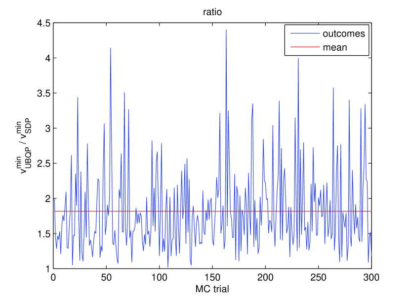
Fig. 1: Upper bound on $v^{\min}_{{\rm QP}}/v^{\min}_{{\rm SDP}}$ for $M=8$, $Q=6$, $N=8$, $300$ realizations of real Gaussian i.i.d. $\mathbf{h}_{i}$ for $i=1,\cdots,M$ in the real case.

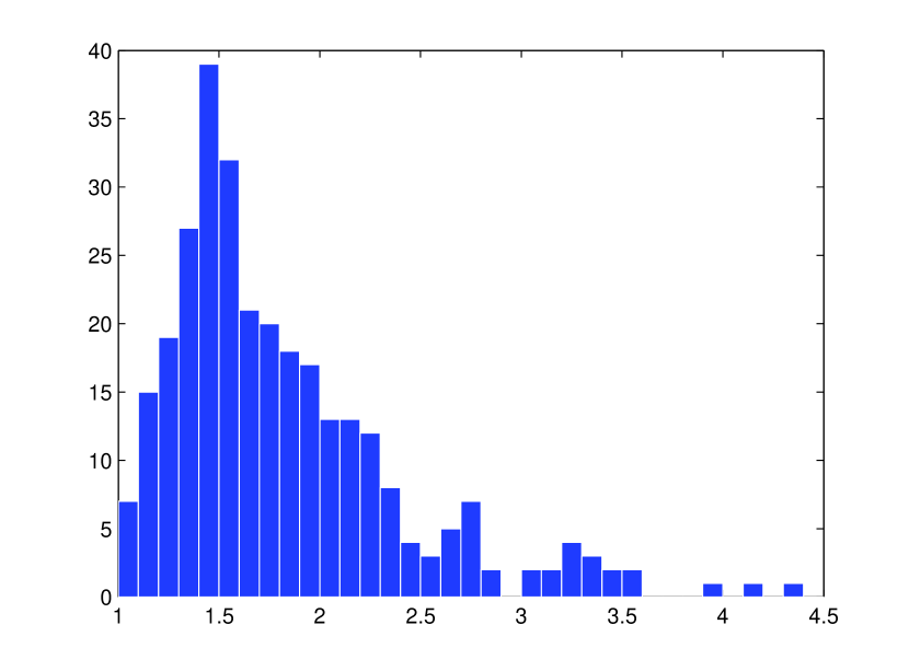
Fig. 2: Histogram of the outcomes in Figure 1.

Table 4: Mean and standard deviation of the approximation ratio over $300$ independent realizations of real Gaussian i.i.d. $\mathbf{h}_{i}$ $(i=1,\cdots,M)$, when $\mathbb{F}=\mathbb{R}$.

$M$	$Q$	$N=4$			$N=8$
		max	mean	Std	max	mean	Std
$M=8$	$Q=M/4$	3.7394	2.0348	0.2266	4.3387	2.0392	0.2948
	$Q=M/2$	3.9420	1.7972	0.1828	3.5232	1.7378	0.1475
	$Q=3M/4$	4.6973	1.7863	0.3921	4.5721	1.8130	0.3428
$M=12$	$Q=M/4$	4.9450	2.2191	0.2451	3.9625	2.1710	0.2304
	$Q=M/2$	5.8068	2.0639	0.4564	4.3483	2.0204	0.3241
	$Q=3M/4$	7.7829	2.5970	1.3075	9.7150	2.8277	1.9578
$M=16$	$Q=M/4$	4.2703	2.2977	0.2410	4.2980	2.2117	0.1972
	$Q=M/2$	7.3115	2.4463	0.9348	7.8240	2.4166	1.1345
	$Q=3M/4$	10.715	3.2272	2.3823	10.621	3.7786	2.8760

Table 5: Mean and standard deviation of upper bound ratio over $300$ independent realizations of real Gaussian i.i.d. $\mathbf{h}_{i}$ $(i=1,\cdots,M)$, when $\mathbb{F}=\mathbb{C}$.

$M$	$Q$	$N=4$			$N=8$
		max	mean	Std	max	mean	Std
$M=8$	$Q=M/4$	4.8049	2.3720	0.2790	4.3579	2.4239	0.2757
	$Q=M/2$	3.7344	1.9308	0.1443	3.4477	1.9243	0.1477
	$Q=3M/4$	2.7549	1.5812	0.0769	2.4477	1.5860	0.0818
$M=12$	$Q=M/4$	4.0557	2.4986	0.1938	3.7851	2.4657	0.1998
	$Q=M/2$	3.2911	2.0301	0.1483	3.2867	2.0567	0.1190
	$Q=3M/4$	2.6007	1.6451	0.0800	3.1609	1.6693	0.0860
$M=16$	$Q=M/4$	3.8170	2.5778	0.1647	4.2616	2.5852	0.1757
	$Q=M/2$	3.6268	2.0908	0.0932	3.7761	2.0729	0.1065
	$Q=3M/4$	2.9218	1.8024	0.1044	3.6056	1.8344	0.1432

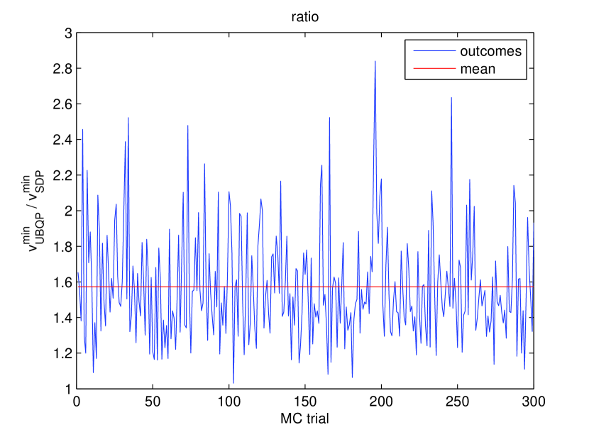
Fig. 3: Upper bound on $v^{\min}_{{\rm QP}}/v^{\min}_{{\rm SDP}}$ for $M=8$, $Q=6$, $N=8$, $300$ realizations of real Gaussian i.i.d. $\mathbf{h}_{i}$ for $i=1,\cdots,M$ in the complex case.

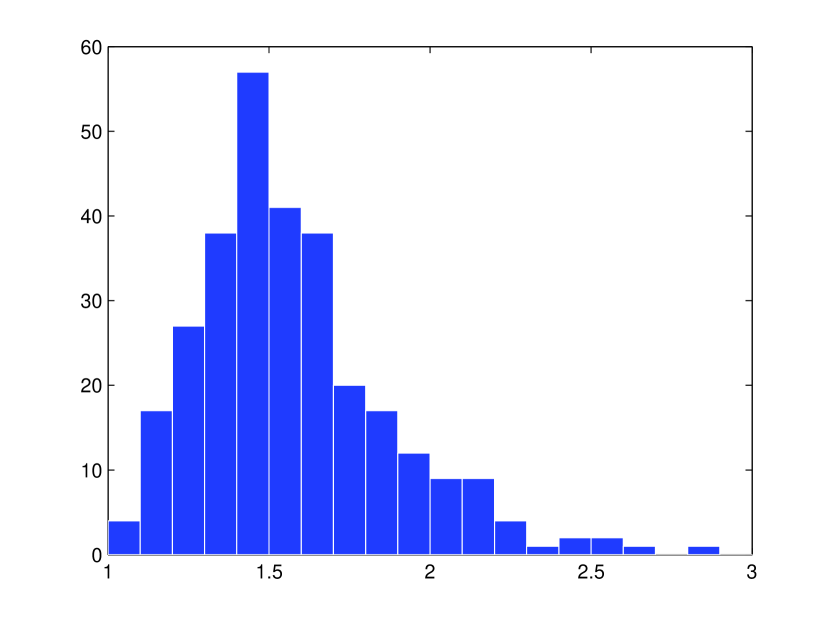
Fig. 4: Histogram of the outcomes in Figure 3.

While theoretical worst-case analysis is very useful, empirical analysis of the ratio $v^{\min}_{{\rm QP}}/v^{\min}_{{\rm SDP}}$ and $v^{\max}_{{\rm QP}}/v^{\max}_{{\rm SDP}}$ through simulations can often provide valuable insights into the true efficacy of the relaxation methods. Throughout this section, we generate the data matrix $\mathbf{H}_{i}$ by using $\mathbf{H}_{i}=\mathbf{h}_{i}\mathbf{h}_{i}^{H}$ $(i=1,\cdots,M)$, with randomly generated vectors $\mathbf{h}_{i}$. The SDP relaxation problems are all solved by CVX [10].

For the minimization model, we test the proposed procedure listed in Table 1 for $\epsilon=0$ and different choices of $M$, $Q$ and $N$. The performance of the algorithm with other choices of $\epsilon$ are similar. The Step S3 and Step S4 are repeated by $T=1000$ independent trials, and the solution generated by $k$th trial is denoted by $(\mathbf{x}^{(2)})^{k}$. Let

$$v^{\min}_{{\rm UBQP}}:=\min_{k=1,\cdots,T}\|(\mathbf{x}^{(2)})^{k}\|^{2}.$$

Clearly $v^{\min}_{{\rm UBQP}}$ is an upper bound for $v^{\min}_{{\rm QP}}$, as a result, $v^{\min}_{{\rm UBQP}}/v^{\min}_{{\rm SDP}}$ can be used as an upper bound of the true approximation ratio (which is difficult to obtain).

Table 4 shows the average ratio (mean) of $v^{\min}_{{\rm UBQP}}/v^{\min}_{{\rm SDP}}$ over 300 independent realizations of i.i.d. real-valued Gaussian $\mathbf{h}_{i}$, $(i=1,\cdots,M)$ for several combinations of $M$, $Q$ and $N$. The maximum value (max) and the standard deviation (Std) of $v^{\min}_{{\rm UBQP}}/v^{\min}_{{\rm SDP}}$ over 300 independent realizations are also shown in Table 4. Table 5 shows the corresponding average value, maximum value and the standard deviation of $v^{\min}_{{\rm UBQP}}/v^{\min}_{{\rm SDP}}$ for $\mathbb{F}=\mathbb{C}$. These results are significantly better than what is predicted by our worst-case analysis. In all test examples, the average values of $v^{\min}_{{\rm UBQP}}/v^{\min}_{{\rm SDP}}$ are lower than $4$ (resp. lower than $3$) when $\mathbb{F}=\mathbb{R}$ (resp. when $\mathbb{F}=\mathbb{C}$).

Figure 1 plots $v^{\min}_{{\rm UBQP}}/v^{\min}_{{\rm SDP}}$ for 300 independent realizations of i.i.d. real valued Gaussian $\mathbf{h}_{i}$ ($i=1,\cdots,M$) for $M=8$, $Q=6$ and $N=8$. Figure 2 shows the corresponding histogram. Figure 3 and Figure 4 show the corresponding results for i.i.d complex-valued circular Gaussian $\mathbf{h}_{i}$ ($i=1,\cdots,M$). Both the mean and the maximum of the upper bound $v^{\min}_{{\rm UBQP}}/v^{\min}_{{\rm SDP}}$ are lower in the complex case.

Moreover, our numerical results also corroborates well with our theoretic analysis. First, the upper bound of the approximation ratio is independent of the dimension of $\mathbf{w}$: the results vary only slightly for $N=4$ and $N=8$ in both real and complex case. Second, from Table 4, it can be shown that for fixed $M$, the maximum value of $v^{\min}_{{\rm UBQP}}/v^{\min}_{{\rm SDP}}$ over 300 independent trials grows as $Q$ increases in all test examples except $M=8$ and $N=8$. It corresponds to the result in Theorem 5. While in Table 5, for fixed $M$, the maximum value of $v^{\min}_{{\rm UBQP}}/v^{\min}_{{\rm SDP}}$ over 300 independent trials becomes smaller as $Q$ increases in all test examples, which is also consistent with the theoretic result listed in Theorem 6.

The above empirical analysis complements our theoretic worst-case analysis of the performance of SDP relaxation for the class of mixed integer QCQP problems considered herein.

5 Conclusion and Discussion

Motivated by important emerging applications in transmit beamforming for joint physical layer multicasting and admission control in wireless networks, this paper proposes new SDP relaxation techniques for two classes of nonconvex quadratic optimization problems with mixed binary and continuous variables. It is shown that these efficient techniques (polynomial time) are guaranteed to provide high quality approximate solutions with a finite approximation ratio that is independent of problem dimension and data matrices. This work extends the existing SDP relaxation techniques for continuous nonconvex QCQPs. Our theoretic analysis provides useful insights on the effectiveness of the new SDP relaxation techniques for this class of mixed integer QCQP problems.

It should be pointed out that our worst-case analysis of SDP relaxation performance is based on a certain structure of the discrete variables in the mixed integer QCQPs. Can we extend the SDP relaxation techniques and the corresponding analysis to more general MBQCQP problems? For the maximization model, such extension is not possible, as the approximation ratio for SDP relaxation can be zero for certain special instances of the problem (see e.g., Example 3.1). For the minimization model, the following counter example suggests that this is also impossible.

Example 5.1. Consider the following general MBQCQP problem in minimization form:

$$\min_{\mathbf{x}\in\mathbb{R}^{n}} \quad\|\mathbf{x}\|^{2}$$

$${\rm s.t.} \quad\mathbf{x}^{H}\mathbf{D}_{i}\mathbf{x}\geq 1,~{}i=1,\cdots,M$$ (85)

$$\quad(\mathbf{x}[j])^{2}=1,~{}j=1,\cdots,l$$

with $l\leq n$ and $\mathbf{D}_{i}$, $i=1,\cdots,M$ being arbitrarily positive semidefinite matrices. The SDP relaxation for this problem can be expressed as

$$\min \quad{\mbox{{Tr}}}[\mathbf{X}]$$

$${\rm s.t.} \quad{\mbox{{Tr}}}[\mathbf{D}_{i}\mathbf{X}]\geq 1,~{}i=1,\cdots,M$$ (86)

$$\quad\mathbf{X}[j,j]=1,~{}j=1,\cdots,l$$

$$\quad\mathbf{X}\succeq 0.$$

We show in the following that SDP relaxation (86) can be very loose for this general case. Let $M=2$, $l=1$, $n=2$, and let

$$\mathbf{D}_{1}=\left[\begin{array}[]{cc}1-\epsilon&\sqrt{\epsilon(1-\epsilon)}\\ \sqrt{\epsilon(1-\epsilon)}&\epsilon\end{array}\right],\qquad\mathbf{D}_{2}=\left[\begin{array}[]{cc}1&-\sqrt{\frac{\epsilon}{2}}\\ -\sqrt{\frac{\epsilon}{2}}&\epsilon\end{array}\right]$$

where $\epsilon$ is some positive constant. It is relatively easy to show that the optimal solution ${\bar{\mathbf{x}}}$ for problem (85) is give by

$$\bar{\mathbf{x}}[1]=1,\quad\bar{\mathbf{x}}[2]=\min\left\{\sqrt{\frac{2}{\epsilon}},\ \frac{\sqrt{1-\epsilon}+1}{\sqrt{\epsilon}}\right\}.$$

Thus, when $\epsilon\rightarrow 0$, we have $\bar{\mathbf{x}}[2]\rightarrow+\infty$, implying $\|\bar{\mathbf{x}}\|^{2}\rightarrow+\infty$. However, it can be easily checked that $\mathbf{X}=\mathbf{I}$ is a feasible solution for the problem (86). Therefore, the optimal solution ${\bar{\mathbf{X}}}$ for (86) should satisfy

$${\mbox{{Tr}}}[{\bar{\mathbf{X}}}]\leq{\mbox{{Tr}}}[\mathbf{I}]=2.$$

This example shows that, for a general MBQCQP problem in minimization form, the approximation ratio can be arbitrarily large, i.e., the worst-case approximation ratio as stated in (29) is $\mu=+\infty$.

As a final remark, we mention that the the approximation bounds obtained in this work are due to the special structures of the problems under consideration. For example, the constraints on the discrete variables are relatively simple. Moreover, the discrete variables and the continuous variables are separable, e.g., there are no cross terms between the discrete and the continuous variables, either in the constraints or the objective. These nice properties allow us to design algorithms that can separately deal with the discrete and the continuous variables.

References

- [1] A. Beck and M. Teboulle, A convex optimization approach for minimizing the ratio of indefinite quadratic functions over an ellipsoid, Math. Program., 118(2009), pp. 13–35.
- [2] A. Ben-Tal, A. Nemirovski, and C. Roos, Robust solutions of uncertain quadratic and conic-quadratic problems, SIAM J. Optim., 13 (2002), pp. 535–560.
- [3] A. Billionnet, S. Elloumi and A. Lambert, Extending the QCR method to general mixed-integer programs, Math. Program., 131(2012), pp. 381–401.
- [4] A. Billionnet, S. Elloumi and M.-C. Plateau, Improving the performance of standard solvers for quadratic 0-1 programs by a tight convex reformulation: the QCR method, Discr. Appl. Math., 157(2009), pp. 1185–1197.
- [5] S. Burer and A. Saxena, The MILP road to MIQCP. In: J. Lee and S. Leyffer (eds.) Mixed-Integer Nonlinear Programming, pp. 373–406. IMA Volumes in Mathematics and its Applications, vol. 154. Berlin: Springer, 2011.
- [6] S. Burer and A. Letchford, Non-convex mixed-integer nonlinear programming: A survey, Manuscript, To appear in Surveys in Operations Research and Management Science, 2012.
- [7] M.A. Duran and I.E. Grossmann, An outer-approximation algorithm for a class of mixed-integer nonlinear programs, Math. Program., 36(1986), pp. 307–339.
- [8] A. M. Frieze and M. Jerrum, Improved approximation algorithms for max k-cut and max bisection, in Proceedings of the 4th International IPCO Conference on Integer Programming and Combinatorial Optimization, London, UK, UK, Springer-Verlag, 1995, pp. 1 C13.
- [9] M. X. Goemans and D. P. Williamson, Improved approximation algorithms for maximum cut and satisfiability problems using semidefinite programming, Journal of ACM, 42 (1995), pp. 1115–1145.
- [10] M. Grant and S. Boyd, CVX: Matlab software for disciplined convex programming, version 1.21, Apr. 2011.
- [11] S. He, Z.-Q. Luo, J. Nie and S. Zhang, Semidefinite relaxation bounds for indefinite homogneous quadratic optimization, SIAM J. Optim., 19(2008), pp. 503–523.
- [12] R.Hemmecke, M.Koppe, J. Lee and R. Weismantel, Nonlinear integer programming, In M. Junger et al (eds.) 50 Years of Integer Programming 1958-2008, pp. 561–618, Berlin: Springer, 2010.
- [13] Y. Huang and S. Zhang, Complex matrix decomposition and quadratic programming, Math. Oper. Res., 32(2007), pp. 758–768.
- [14] M. Kisialiou and Z.-Q. Luo, Probabilistic Analysis of Semidefinite Relaxation for Binary Quadratic Minimization, SIAM J. Optim., 20 (2010), pp. 1906–1922.
- [15] M. Koppe, On the complexity of nonlinear mixed integer optimization, In J. Lee and S. Leyffer (eds.) Mixed-integer Nonlinear Programming, pp. 533–558. IMA Volumes in Mathematics and its Applications, Vol. 154, Berlin: Springer, 2011.
- [16] Ya-Feng Liu, Yu-Hong Dai and Zhi-Quan Luo, Joint power and admission control via linear programming deflation, Proceedings of ICASSP, (2012), pp. 2873–2876.
- [17] Z.-Q. Luo, N. D. Sidiropoulos, P. Tseng, and S. Zhang, Approximation bounds for quadratic optimization with homogeneous quadratic constraints, SIAM J. Optim., 18 (2007), pp. 1–28.
- [18] Z.-Q. Luo and W.-K. Ma and So, A.M.-C. and Y. Ye and S. Zhang, Semidefinite Relaxation of Quadratic Optimization Problems, IEEE Signal Processing Magazine, 27 (2010), pp. 20–34.
- [19] Matskani, E. and Sidiropoulos, N. and Z.-Q. Luo and Tassiulas, L., Convex approximation techniques for joint multiuser downlink beamforming and admission control, IEEE Transactions on Wireless Communications, 7 (2008), pp. 2682–2693.
- [20] E. Matskani, N. D. Sidiropoulos, Z.-Q. Luo, and L. Tassiulas, Efficient batch and adaptive approximation algorithms for joint multicast beamforming and admission control, IEEE Transactions on Signal Processing, 57 (2009), pp. 4882–4894.
- [21] A. Nemirovski, C. Roos, and T. Terlaky, On maximization of quadratic form over intersection of ellipsoids with common center, Math. Program., 86 (1999), pp. 463–473.
- [22] G. Pataki, On the rank of extreme matrices in semidefinite programs and the multiplicity of optimal eigenvalues, Math. oper. Res., 23 (1998), pp. 339–358.
- [23] A. Saxena, P. Bonami and J. Lee, Convex relaxations of non-convex mixed integer quadratically constrained programs: extended formulations, Math. Program., 124(2010), pp. 383-411.
- [24] A. Saxena, P. Bonami and J. Lee, Convex relaxations of non-convex mixed integer quadratically constrained programs: projected formulations, Math. Program., 130(2011), pp. 359-413.
- [25] N. D. Sidiropoulos, T. N. Davidson, and Z.-Q. Luo, Transmit beamforming for physical-layer multicasting, IEEE Transactions on Signal Processing, 54 (2006), pp. 2239–2251.
- [26] A. M.-C. So, Y. Ye, and J. Zhang, A unified theorem on sdp rank reduction, Mathematics of Operations Research, 33 (2008), pp. 910–920.
- [27] A. M.-C. So, Probabilistic Analysis of the Semidefinite Relaxation Detector in Digital Communications, Proc. 21st SODA, (2010), pp. 698–711.
- [28] R.A. Stubbs and S. Mehrotra, A branch-and-cut method for 0-1 mixed convex programming, Math. Program., 86(1999), pp. 515–532.
- [29] T.Westerlund and F. Pettersson, A cutting plane method for solving convex MINLP problems, Comput. and Chem. Eng., 19(1995), pp. 131–136.
- [30] Y. Ye, A .699-approximation algorithm for max-bisection, Mathematical Programming, 90 (2001), pp. 101–111.
- [31] S. Zhang, Quadratic maximization and semidefinite relaxation, Mathematical Programming, 87 (2000), pp. 453–465.
- [32] S. Zhang and Y. Huang, Complex quadratic optimization and semidefinite programming, SIAM Journal on Optimization, 16 (2004), pp. 871–890.