Breaking the Small Cluster Barrier of Graph Clustering

Abstract

This paper investigates graph clustering in the planted cluster model in the presence of small clusters. Traditional results dictate that for an algorithm to provably correctly recover the clusters, all clusters must be sufficiently large (in particular, $\tilde{\Omega}(\sqrt{n})$ where $n$ is the number of nodes of the graph). We show that this is not really a restriction: by a more refined analysis of the trace-norm based matrix recovery approach proposed in Jalali et al. (2011) and Chen et al. (2012), we prove that small clusters, under certain mild assumptions, do not hinder recovery of large ones. Based on this result, we further devise an iterative algorithm to recover almost all clusters via a “peeling strategy”, i.e., recover large clusters first, leading to a reduced problem, and repeat this procedure. These results are extended to the partial observation setting, in which only a (chosen) part of the graph is observed. The peeling strategy gives rise to an active learning algorithm, in which edges adjacent to smaller clusters are queried more often as large clusters are learned (and removed).

From a high level, this paper sheds novel insights on high-dimensional statistics and learning structured data, by presenting a structured matrix learning problem for which a one shot convex relaxation approach necessarily fails, but a carefully constructed sequence of convex relaxations does the job.

1 Introduction

This paper considers a classic problem in machine learning and theoretical computer science, namely graph clustering, i.e., given an undirected unweighted graph, partition the nodes into disjoint clusters, so that the density of edges within one cluster is higher than those across clusters. Graph clustering arises naturally in many application across science and engineering. Some prominent examples include community detection in social network Mishra et al. (2007), submarket identification in E-commerce and sponsored search Yahoo!-Inc (2009), and co-authorship analysis in analyzing document database Ester et al. (1995), among others. From a purely binary classification theoretical point of view, the edges of the graph are (noisy) labels of similarity or affinity between pairs of objects, and the concept class consists of clusterings of the objects (encoded graphically by identifying clusters with cliques).

Many theoretical results in graph clustering (e.g., Boppana, 1987; Chen et al., 2012; McSherry, 2001) consider the planted partition model, in which the edges are generated randomly; see Section 1.1 for more details. While numerous different methods have been proposed, their performance guarantees all share the following manner – under certain condition of the density of edges (within clusters and across clusters), the proposed method succeeds to recover the correct clusters exactly if all clusters are larger than a threshold size, typically $\tilde{\Omega}(\sqrt{n})$.

In this paper, we aim to break this small cluster barrier of graph clustering. Correctly identifying extremely small clusters is inherently hard as they are easily confused with “fake” clusters generated by noisy edges, and is not the focus of this paper. Instead, in this paper we investigate a question that has not been addressed before: Can we still recover large clusters in the presence of small clusters? Intuitively, this should be doable. To illustrate, consider an extreme example where the given graph $G$ consists two disjoint subgraphs $G_{1}$ and $G_{2}$, where $G_{1}$ is a graph that can be correctly clustered using some existing method, and $G_{2}$ is a small-size clique. $G$ certainly violates the minimum cluster size requirement of previous results, but why should $G_{2}$ spoil our ability to cluster $G_{1}$?

Our main result confirms this intuition. We show that the cluster size barrier arising in previous work (e.g., Chaudhuri et al., 2012; Bollobás and Scott, 2004; Chen et al., 2012; McSherry, 2001) is not really a restriction, but rather an artifact of the attempt to solve the problem in a single shot using convex relaxation techniques. Using a more careful analysis, we prove that the mixed trace-norm and $\ell_{1}$ based convex formulation, initially proposed in Jalali et al. (2011), can recover clusters of size $\tilde{\Omega}(\sqrt{n})$ even in the presence of smaller clusters. That is, small clusters do not interfere with recovery of the big clusters.

The main implication of this result is that one can apply an iterative “peeling” strategy, recovering smaller and smaller clusters. The intuition is simple – suppose the number of clusters is limited, then either all clusters are large, or the sizes of the clusters vary significantly. The first case is obviously easy. The second one is equally easy: use the aforementioned convex formulation, the larger clusters can be correctly identified. If we remove all nodes from these larger clusters, the remaining subgraph contains significantly fewer nodes than the original graph, which leads to a much lower threshold on the size of the cluster for correct recovery, making it possible for correctly clustering some smaller clusters. By repeating this procedure, indeed, we can recover the cluster structure for almost all nodes with no lower bound on the minimal cluster size. We summarize our main contributions and techniques:

(1) We provide a refined analysis of the mixed trace norm and $\ell_{1}$ convex relaxation approach for exact recovery of clusters proposed in Jalali et al. (2011) and Chen et al. (2012), focusing on the case where small clusters exist. We show that in the classical planted partition settings Boppana (1987), if each cluster is either large (more precisely, of size at least $x\approx\sqrt{n}\log^{2}n$) or small (of size at most $x/\log^{2}n$), then with high probability, this convex relaxation approach correctly identifies all big clusters while “ignoring” the small ones. Notice that the multiplicative gap between the two thresholds is logarithmic w.r.t. $n$. In addition, it is possible to arbitrarily increase $x$, thus turning a “knob” in quest of an interval $(x/\log^{2}n,x)$ that is disjoint from the set of cluster sizes. The analysis is done by identifying a certain feasible solution to the convex program and proving its almost sure optimality using a careful construction of a dual certificate. This feasible solution easily identifies the big clusters. This method has been performed before only in the case where all clusters are of size $\geq x$.

(2) We provide a converse of the result just described. More precisely, we show that if for some value of the knob $x$ an optimal solution appears to look as if the interval $(x/\log^{2}n,x)$ were indeed free of cluster sizes, then the solution is useful (in the sense that it correctly identifies big clusters) even if this weren’t the case.

(3) The last two points imply that if some interval of the form $(x/\log^{2}n,x)$ is free of cluster sizes, then an exhaustive search of this interval will constructively find big clusters (though not necessarily for that particular interval). This gives rise to an iterative algorithm, using a “peeling strategy”, to recover smaller and smaller clusters that are otherwise impossible to recover. Using the “knob”, we prove that as long as the number of clusters is bounded by $\Omega(\log n/\log\log n)$, regardless of the cluster sizes, we can correctly recover the cluster structure for an overwhelming fraction of nodes. To the best of our knowledge, this is the first result of provably correct graph clustering without any assumptions on the cluster sizes.

(4) We extend the result to the partial observation case, where only a faction of similarity labels (i.e., edge/no edge) is known. As expected, smaller observation rates allow identification of larger clusters. Hence, the observation rate serves as the “knob”. This gives rise to an active learning algorithm for graph clustering based on adaptively increasing the rate of sampling in order to hit a “forbidden interval” free of cluster sizes, and concentrating on smaller inputs as we identify big clusters and peel them off.

Beside these technical contributions, this paper provides novel insights into low-rank matrix recovery and more generally high-dimensional statistics, where data are typically assumed to obey certain low-dimensional structure. Numerous methods have been developed to exploit this a priori information so that a consistent estimator is possible even when the dimensionality of data is larger than the number of samples. Our result shows that one may combine these methods with a “peeling strategy” to further push the envelope of learning structured data – By iteratively recovering the easier structure and then reducing the problem size, it is possible to learn structures that are otherwise difficult using previous approaches.

1.1 Previous work

The literature of graph clustering is too vast for a detailed survey here; we concentrate on the most related work, and in specific those provide theoretical guarantees on cluster recovery.

Planted partition model: The setup we study is the classical planted partition model Boppana (1987), also known as the stochastic block model Rohe et al. (2011). Here, $n$ nodes are partitioned into subsets, referred as the “true clusters”, and a graph is randomly generated as follows: for each pair of nodes, depending on whether they belong to a same subset, an edge connecting them is generated with a probability $p$ or $q$ respectively. The goal is to correctly recover the clusters given the random graph. The planted partition model has been studied as early as 1980’s Boppana (1987). Earlier work focused on the 2-partition or more generally $l$-partition case, i.e., the minimal cluster size is $\Theta(n)$ Boppana (1987); Condon and Karp (2001); Carson and Impagliazzo (2001); Bollobás and Scott (2004). Recently, several works have proposed methods to handle sublinear cluster sizes. These works can be roughly classified into three approaches: randomized algorithms  (e.g., Shamir and Tsur, 2007), spectral clustering (e.g., McSherry, 2001; Giesen and Mitsche, 2005; Chaudhuri et al., 2012; Rohe et al., 2011)), and low-rank matrix decomposition Jalali et al. (2011); Chen et al. (2012); Ames and Vavasis (2011); Oymak and Hassibi (2011). While these work differs in the methodology, they all impose constraints on the size of the minimum true cluster – the best result up-to-date requires it to be $\tilde{\Omega}(\sqrt{n})$.

Correlation Clustering This problem, originally defined by Bansal, Blum and Chawla Bansal et al. (2004), also considers graph clustering but in an adversarial noise setting. The goal there is to find the clustering minimizing the total disagreement (intercluster edges plus intracluster nonedges), without there being necessarily a notion of true clustering (and hence no “exact recovery”). This problem is usually studied in the combinatorial optimization framework and is known to be NP-Hard to approximate to within some constant factor. Prominent work includes Demaine et al. (2006); Ailon et al. (2008); Charikar et al. (2005). A PTAS is known in case the number of clusters is fixed Giotis and Guruswami (2006).

Low rank matrix decomposition via trace norm: Motivated from robust PCA, it has recently been shown Chandrasekaran et al. (2011); Candès et al. (2011), that it is possible to recover a low-rank matrix from sparse errors of arbitrary magnitude, where the key ingredient is using trace norm (aka nuclear norm) as a convex surrogate of the rank. A similar result is also obtained when the low rank matrix is corrupted by other types of noise Xu et al. (2012).

Of particular relevance to this paper is Jalali et al. (2011) and Chen et al. (2012), where the authors apply this approach to graph clustering, and specifically to the planted partition model. Indeed, Chen et al. (2012) achieve state-of-art performance guarantees for the planted partition problem. However, they don’t overcome the $\tilde{\Omega}(\sqrt{n})$ minimal cluster size lower bound.

Active learning/Active clustering Another line of work that motivates this paper is study of active learning algorithms (a settings in which labeled instances are chosen by the learner, rather than by nature), and in particular active learning for clustering. The most related work is Ailon et al. (2012), who investigated active learning for correlation clustering. The authors obtain a $(1+\varepsilon)$-approximate solution with respect to the optimal, while (actively) querying no more than $O(n\operatorname{poly}(\log n,k,\varepsilon^{-1}))$ edges. The result imposed no restriction on cluster sizes and hence inspired this work, but differs in at least two major ways. First, Ailon et al. (2012) did not consider exact recovery as we do. Second, their guarantees fall in the ERM (Empirical Risk Minimization) framework, with no running time guarantees. Our work recovers true cluster exactly using a convex relaxation algorithm, and is hence computationally efficient. The problem of active learning has also been investigated in other clustering setups including clustering based on distance matrix Voevodski et al. (2012); Shamir and Tishby (2011), and hierarchical clustering Eriksson et al. (2011); Krishnamurthy et al. (2012). These setups differ from ours and cannot be easily compared.

2 Notation and Setup

Throughout, $V$ denotes a ground set of elements, which we identify with the set $[n]=\{1,\dots,n\}$. We assume a true ground truth clustering of $V$ given by a pairwise disjoint covering $V_{1},\dots,V_{k}$, where $k$ is the number of clusters. We say $i\sim j$ if $i,j\in V_{a}$ for some $a\in[k]$, otherwise $i\not\sim j$. We let $n_{i}=|V_{i}|$ for all $i\in[k]$. For any $i\in[n]$, $\langle i\rangle$ is the unique index satisfying $i\in V_{\langle i\rangle}$.

For a matrix $X\in\mathbb{R}^{n\times n}$ and a subset $S\subseteq[n]$ of size $m$, the matrix $X[S]\in\mathbb{R}^{m\times m}$ is the principal minor of $X$ corresponding to the set of indexes $S$. For a matrix $M$, $\Gamma(M)$ denotes the support of $M$, namely, the set of index pairs $(i,j)$ such that $M(i,j)\neq 0$.

The ground truth clustering matrix, denoted $K^{*}$, is defined so that $K^{*}(i,j)=1$ is $i\sim j$, otherwise $0$. This is a block diagonal matrix, each block consisting of $1$’s only. Its rank is $k$. The input is a symmetric matrix $A$, a noisy version of $K^{*}$. It is generated using the well known planted clustering model, as follows. There are two fixed edge probabilities, $p>q$. We think of $A$ as the adjacency matrix of an undirected random graph, where edge $(i,j)$ is in the graph for $i>j$ with probability $p$ if $i\sim j$, otherwise with probability $q$, independent of other choices. The error matrix is denoted by $B^{*}:=A-K^{*}$. We let $\Omega:=\Gamma(B^{*})$ denote the noise locations.

Note that our results apply to the more practical case in which the edge probability of $(i,j)$ is $p_{ij}$ for each $i\sim j$ and $q_{ij}$ for $i\not\sim j$, as long as $(\min p_{ij})=:p>q:=(\max q_{ij})$.

3 Results

We remind the reader that the trace norm of a matrix is the sum of its singular values, and we define the $\ell_{1}$ norm of a matrix $M$ to be $\|M\|_{1}=\sum_{ij}|M(ij)|$. Consider the following convex program, combining the trace norm of a matrix variable $K$ with the $\ell_{1}$ norm of another matrix variable $B$ using two parameters $c_{1},c_{2}$ that will be determined later:

$$\mbox{(CP1) }\min \left\|K\right\|_{*}+c_{1}\left\|\mathcal{P}_{\Gamma(A)}B\right\|_{1}+c_{2}\left\|\mathcal{P}_{\Gamma(A)^{c}}B\right\|_{1}$$

s.t. $$K+B=A$$

$$0\leq K_{ij}\leq 1,\forall(i,j).$$

Theorem 1.

There exist constants $b_{1},b_{3},b_{4}>0$ such that the following holds with probability at least $1-n^{-3}$. For any parameter $\kappa\geq 1$ and $t\in[\frac{1}{4}p+\frac{3}{4}q,\frac{3}{4}p+\frac{1}{4}q]$, define

$$\ell_{\sharp}=b_{3}\frac{\kappa\sqrt{p(1-q)n}}{p-q}\log^{2}n\ \ \ell_{\flat}=b_{4}\frac{\kappa\sqrt{p(1-q)n}}{p-q}\ .$$ (1)

If for all $i\in[k]$, either $n_{i}\geq\ell_{\sharp}$ or $n_{i}\leq\ell_{\flat}$ and if $(\hat{K},\hat{B})$ is an optimal solution to (CP1), with

$$c_{1}=\frac{b_{1}}{\kappa\sqrt{n\log n}}\sqrt{\frac{1-t}{t}}\ \ \ c_{2}=\frac{b_{1}}{\kappa\sqrt{n\log n}}\sqrt{\frac{t}{1-t}}\ ,$$ (2)

then $(\hat{K},\hat{B})=({\mathcal{P}}_{\sharp}K^{*},A-\hat{K})$, where for a matrix $M$, ${\mathcal{P}}_{\sharp}M$ is the matrix defined by

$$({\mathcal{P}}_{\sharp}M)(i,j)=\begin{cases}M(i,j)&\max\{n_{\langle i\rangle},n_{\langle j\rangle}\}\geq\ell_{\sharp}\\ 0&\mbox{otherwise}\end{cases}\ .$$

(Note that by the theorem’s premise, $\hat{K}$ is the matrix obtained from $K^{*}$ after zeroing out blocks corresponding to clusters of size at most $\ell_{\flat}$.) The proof is based on Chen et al. (2012) and is deferred to the supplemental material due to lack of space. The main novelty in this work compared to previous work is the treatment of small clusters of size at most $\ell_{\flat}$, whereas in previous work only large clusters were treated, and the existence of small clusters did not allow recovery of the big clusters.

Definition 2.

An $n\times n$ matrix $K$ is a partial clustering matrix if there exists a collection of pairwise disjoint sets $U_{1},\dots,U_{r}\subseteq[n]$ (the induced clusters) such that $K(i,j)=1$ if and only if $i,j\in U_{s}$ for some $s\in[r]$, otherwise $0$. If $K$ is a partial clustering matrix then $\sigma_{\operatorname{min}}(K)$ is defined as $\min_{i=1}^{r}|U_{i}|$.

The definition is depicted in Figure 1. Theorem 1 tells us that by choosing $\kappa$ (and hence $c_{1}$, $c_{2}$) properly such that no cluster size falls in the range $(\ell_{\flat},\ell_{\sharp})$, the unique optimal solution $(\hat{K},\hat{B})$ to convex program (CP1) is such that $\hat{K}$ is a partial clustering induced by big ground truth clusters.

In order for this fact to be useful algorithmically, we also need a type of converse: there exists an event with high probability (in the random process generating the input), such that for all values of $\kappa$, if an optimal solution to the corresponding (CP1) looks like the solution $(\hat{K},\hat{B})$ defined in Theorem 1, then the blocks of $\hat{K}$ correspond to actual clusters.

Black represents $1$, white represents $0$. $\sigma_{\operatorname{min}}(K)$ is the side length of the smallest black square.

Figure 1: A partial clusering matrix $K$.

Theorem 3.

There exists constants $C_{1},C_{2}>0$ such that with probability at least $1-n^{-2}$, the following holds. For all $\kappa\geq 1$ and $t\in[\frac{3}{4}q+\frac{1}{4}p,\frac{1}{4}q+\frac{3}{4}p]$, if $(K,B)$ is an optimal solution to (CP1) with $c_{1},c_{2}$ as defined in Theorem 1, and additionally $K$ is a partial clustering induced by $U_{1},\dots,U_{r}\subseteq V$, and also

$$\sigma_{\operatorname{min}}(K)\geq\max\left\{\frac{C_{1}k\log n}{(p-q)^{2}},\frac{C_{2}\kappa\sqrt{p(1-q)n\log n}}{p-q}\right\}\ ,$$ (3)

then $U_{1},\dots,U_{r}$ are actual ground truth clusters, namely, there exists an injection $\phi:[r]\mapsto[k]$ such that $U_{i}=V_{\phi(i)}$ for all $i\in[r]$.

(Note: Our proof of Theorem 3 uses Hoeffding tail bounds for simplicity, which are tight for $p,q$ bounded away from $0$ and $1$. Bernstein tail bounds can be used to strengthen the result for other classes of $p,q$. We elaborate on this in Section 3.1.)

The combination of Theorems 1 and 3 implies that, as long as there exists a relatively small interval which is disjoint from the set of cluster sizes, and such that at least one cluster size is larger than this interval (and large enough), we can recover at least one (large) cluster using (CP1). This is made clear in the following.

Corollary 4.

Assume we have a guarantee that there exists a number $\alpha\geq b_{4}\frac{\sqrt{p(1-q)n}}{p-q}$, such that no cluster size falls in the interval $(\alpha,\frac{b_{3}}{b_{4}}\alpha\log^{2}n)$ and at least one cluster size is of size at least $s:=\max\{\frac{b_{3}}{b_{4}}\alpha\log^{2}n,(C_{1}k\log n)/(p-q)^{2},C_{2}\sqrt{p(1-q)n\log n}/(p-q)\}$. Then with probability at least $1-n^{-2}$, we can recover at least one cluster of size at least $s$ efficiently by solving (CP1) with $\kappa=\alpha/\left(b_{4}\frac{\sqrt{p(1-q)n}}{p-q}\right)$.

Of course we do not know what $\alpha$ (and hence $\kappa$) is. We could exhaustively search for a $\kappa\geq 1$ and hope to recover at least one large cluster. A more interesting question is, when is such a $\kappa$ guaranteed to exist? Let $g=\frac{b_{3}}{b}{b_{4}}\log^{2}n$. The number $g$ is the (multiplicative) gap size, equaling the ratio between $\ell_{\sharp}$ and $\ell_{\flat}$ (for any $\kappa$). If the number of clusters $k$ is a priori bounded by some $k_{0}$, we both ensure that there is at least one cluster of size $n/k_{0}$, and by the pigeonhole principle, that one of the intervals in the sequence $(n/gk_{0},n/k_{0}),(n/g^{2}k_{0},n/gk_{0}),\dots,(n/g^{k_{0}+1}k_{0},n/g^{k_{0}}k_{0})$. is disjoint of cluster sizes. If, in addition, the smallest interval in the sequence is not too small and $n/k_{0}$ is not too small so that Corollary 4 holds, then we are guaranteed to recover at least one cluster using Algorithm 1. We find this condition difficult to work with. An elegant, useful version of the idea is obtained if we assume $p,q$ are some fixed constants. As the following lemma shows, it turns our that in this regime, $k_{0}$ can be assumed to be almost logarithmic in $n$ to ensure recovery of at least one cluster. In what follows, notation such as $C(p,q),C_{3}(p,q),\dots$ denotes universal positive functions that depend on $p,q$ only.

Lemma 5.

There exists $C_{3}(p,q),C_{4}(p,q),C_{5}>0$ such that the following holds. Assume that $n>C_{4}(p,q)$, and that we are guaranteed that $k\leq k_{0}$, where $k_{0}=\frac{C_{3}(p,q)\log n}{\log\log n}$. Then with probability at least $1-n^{-2}$ Algorithm 1 will recover at least one cluster in at most $C_{5}k_{0}$ iterations.

The proof is deferred to the supplemental material section. Lemma 5 ensures that by trying at most a logarithmic number of values of $\kappa$, we can recover at least one large cluster, assuming the number of clusters is roughly logarithmic in $n$. The next proposition tells us that as long as this step recovers the clusters covering at most all but a vanishing fraction of elements, the step can be repeated.

Proposition 6.

A pair of numbers $(n^{\prime},k^{\prime})$ is called good if $n^{\prime}\leq n,k^{\prime}\leq k$ and $k^{\prime}\leq\frac{C_{3}(p,q)\log n^{\prime}}{\log\log n}$. If $(n^{\prime},k^{\prime})$ is good, then $(n^{\prime\prime},k^{\prime\prime})$ is good for all $n^{\prime\prime},k^{\prime\prime}$ satisfying $n^{\prime}\geq n^{\prime\prime}\geq n^{\prime}/(\log n)^{1/C_{3}(p,q)}$ and $k^{\prime}-1\geq k^{\prime\prime}\geq 1$.

The proof is trivial. The proposition implies an inductive process in which at least one big (with respect to the current unrecovered size) cluster can be efficiently removed as long as the previous step recovered at most a $(1-(\log n)^{-1/C_{3}(p,q)})$-fraction of its input. Combining, we proved the following:

Theorem 7.

Assume $n,k$ satisfy the requirements of Lemma 5. Then with probability at least $1-2n^{-2}$ Algorithm 2 recovers clusters covering all but at most a $((\log n)^{-1/C_{3}(p-q)})$ fraction of the input in the full observation case, without any restriction of the minimal cluster size. Moreover, if we assume that $k$ is bounded by a constant $k_{0}$, then the algorithm will recover clusters covering all but a constant number of input elements.

Algorithm 1 ${\operatorname{RecoverBigFullObs}}(V,A,p,q)$

  require: ground set $V$, $A\in\mathbb{R}^{V\times V}$, probs $p,q$

  $n\leftarrow|V|$

  $t\leftarrow\frac{1}{4}p+\frac{3}{4}q$ (or anything in $[\frac{1}{4}p+\frac{3}{4}q,\frac{3}{4}p+\frac{1}{4}q]$)

  $\ell_{\sharp}\leftarrow n$, $g\leftarrow\frac{b_{3}}{b_{4}}\log^{2}n$

  // (If have prior bound $k_{0}$ on num clusters,

  //    take $\ell_{\sharp}\leftarrow n/k_{0}$)

  while $\ell_{\sharp}\geq\max\left\{\frac{C_{1}k\log n}{(p-q)^{2}},\frac{C_{2}\sqrt{p(1-q)n\log n}}{p-q}\right\}$ do

     solve for $\kappa$ using (1), set $c_{1},c_{2}$ as in (2)

     $(\hat{K},\hat{B})\leftarrow$ optimal solution to (CP1) with $c_{1},c_{2}$

     if $\hat{K}$ partial clustering matrix with $\sigma_{\operatorname{min}}(\hat{K})\geq\ell_{\sharp}$ then

        return induced clusters $\{U_{1},\dots,U_{r}\}$ of $\hat{K}$

     end if

     $\ell_{\sharp}\leftarrow\ell_{\sharp}/g$

  end while

  return $\emptyset$

Algorithm 2 $\operatorname{RecoverFullObs}(V,A,p,q)$

  require: ground set $V$, matrix $A\in\mathbb{R}^{V\times V}$, probs $p,q$

  $\{U_{1},\dots,U_{r}\}\leftarrow{\operatorname{RecoverBigFullObs}}(V,A,p,q)$

  $V^{\prime}\leftarrow[n]\setminus(U_{1}\cup\cdots\cup U_{r})$

  if $r=0$ then

     return $\emptyset$

  else

     return $\operatorname{RecoverFullObs}(V^{\prime},A[V^{\prime}],p,q)\cup\{U_{1},\dots,U_{r}\}$

  end if

3.1 Partial Observations

We now consider the case where the input matrix $A$ is not given to us in entirety, but rather that we have oracle access to $A(i,j)$ for $(i,j)$ of our choice. Unobserved values are formally marked with $A(i,j)=?$.

Consider a more particular setting in which the edge probabilities defining $A$ are $p^{\prime}$ (for $i\sim j$) and $q^{\prime}$ (for $i\not\sim j$), and we observe $A(i,j)$ with probability $\rho$, for each $i,j$, independently. More precisely: For $i\sim j$ we have $A(i,j)=1$ with probability $\rho p^{\prime}$, $0$ with probability $\rho(1-p^{\prime})$ and $?$ with remaining probability. For $i\not\sim j$ we have $A(i,j)=1$ with probability $\rho q^{\prime}$, $0$ with probability $\rho(1-q^{\prime})$ and $?$ with remaining probability. Clearly, by pretending that the values $?$ in $A$ are $0$, we emulate the full observation case with $p=\rho p^{\prime}$, $q=\rho q^{\prime}$.

Of particular interest is the case in which $p^{\prime},q^{\prime}$ are held fixed and $\rho$ tends to zero as $n$ grows. In this regime, by varying $\rho$ and fixing $\kappa=1$, Theorem 1 implies the following:

Corollary 8.

There exist constants $b_{1}(p^{\prime},q^{\prime}),b_{3}(p^{\prime},q^{\prime}),b_{4}(p^{\prime},q^{\prime}),b_{5}(p^{\prime},q^{\prime})>0$ such that for any sampling rate parameter $\rho$ the following holds with probability at least $1-n^{-3}$. define

$$\ell_{\sharp}=b_{3}(p^{\prime},q^{\prime})\frac{\sqrt{n}}{\sqrt{\rho}}\log^{2}n\ \ \ \ \ \ \ \ell_{\flat}=b_{4}(p^{\prime},q^{\prime})\frac{\sqrt{n}}{\sqrt{\rho}}\ .$$

If for all $i\in[k]$, either $n_{i}\geq\ell_{\sharp}$ or $n_{i}\leq\ell_{\flat}$ and if $(\hat{K},\hat{B})$ is an optimal solution to (CP1), with

$$c_{1} = \frac{b_{1}(p^{\prime},q^{\prime})}{\sqrt{n\log n}}\sqrt{\frac{1-b_{5}(p^{\prime},q^{\prime})\rho}{b_{5}(p^{\prime},q^{\prime})\rho}}$$

$$c_{2} = \frac{b_{1}(p^{\prime},q^{\prime})}{\sqrt{n\log n}}\sqrt{\frac{b_{5}(p^{\prime},q^{\prime})}{1-b_{5}(p^{\prime},q^{\prime})\rho}}\ ,$$

then $(\hat{K},\hat{B})=({\mathcal{P}}_{\sharp}K^{*},A-\hat{K})$, where ${\mathcal{P}}_{\sharp}$ is as defined in Theorem 1.

(Note: We’ve abused notation by reusing previously defined global constants (e.g. $b_{1}$) with global functions of $p^{\prime},q^{\prime}$ (e.g. $b_{1}(p^{\prime},q^{\prime})$).) Notice now that the observation probability $\rho$ can be used as a knob for controlling the cluster sizes we are trying to recover, instead of $\kappa$. We would also like to obtain a version of Theorem 3. In particular, we would like to understand its asymptotics as $\rho$ tends to $0$.

Theorem 9.

There exist constants $C_{1}(p^{\prime},q^{\prime}),C_{2}(p^{\prime},q^{\prime})>0$ such that for all observation rate parameters $\rho\leq 1$, the following holds with probability at least $1-n^{-2}$. If $(K,B)$ is an optimal solution to (CP1) with $c_{1},c_{2}$ as defined in Theorem 8, and additionally $K$ is a partial clustering induced by $U_{1},\dots,U_{r}\subseteq V$, and also

$$\sigma_{\operatorname{min}}(K)\geq\max\left\{\frac{C_{1}(p^{\prime},q^{\prime})k\log n}{\rho},\frac{C_{2}(p^{\prime},q^{\prime})\sqrt{n\log n}}{\sqrt{\rho}}\right\}\ ,$$ (4)

then $U_{1},\dots,U_{r}$ are actual ground truth clusters, namely, there exists an injection $\phi:[r]\mapsto[k]$ such that $U_{i}=V_{\phi(i)}$ for all $i\in[r]$.

The proof can be found in the supplemental material. Using the same reasoning as before, we derive the following:

Theorem 10.

Let $g=b_{3}(p^{\prime},q^{\prime})/b_{4}(p^{\prime},q^{\prime})\log^{2}n$ (with $b_{3}(p^{\prime},q^{\prime}),b_{4}(p^{\prime},q^{\prime})$ defined in Corollary 8). There exists a constant $C_{4}(p^{\prime},q^{\prime})$ such that the following holds. Assume the number of clusters $k$ is bounded by some known number $k_{0}\leq C_{4}(p^{\prime},q^{\prime})(\log n)/(\log\log n)$. Let $\rho_{0}=\frac{b_{3}(p^{\prime},q^{\prime})^{2}k_{0}^{2}\log^{4}n}{n}$. Then there exists $\rho$ in the set $\{\rho_{0},\rho g,\dots,\rho g^{k_{0}}\}$ for which, if $A$ is obtained with observation rate $\rho$ (zeroing $?$’s), then with probability at least $1-n^{-2}$, any optimal solution $(K,B)$ to (CP1) with $c_{1},c_{2}$ from Corollary 8 satisfies (4).

(Note that the upper bound on $k_{0}$ ensures that $\rho g^{k_{0}}$ is a probability.) The theorem is proven using a simple pigeonhole principle, noting that one of the intervals $(\ell_{\flat}(\rho),\ell_{\sharp}(\rho))$ must be disjoint from the set of cluster sizes, and there is at least one cluster of size at least $n/k_{0}$. The theorem, together with Corollary 8 and Theorem 9 ensures the following. On one end of the spectrum, if $k_{0}$ is a constant (and $n$ is large enough), then with high probability we can recover at least one large cluster (of size at least $n/k_{0}$) after querying no more than

$$O\left(nk_{0}^{2}\left(\frac{b_{3}(p^{\prime},q^{\prime})}{b_{4}(p^{\prime},q^{\prime})}\log^{2}n\right)^{2k_{0}}\log^{4}n\right)$$ (5)

values of $A(i,j)$. On the other end of the spectrum, if $k_{0}\leq\delta(\log n)/(\log\log n)$ and $n$ is large enough (exponential in $1/\delta$), then we can recover at least one large cluster after querying no more than $n^{1+O(\delta)}$ values of $A(i,j)$. (We omit the details of the last fact from this version.) This is summarized in the following:

Theorem 11.

Assume an upper bound $k_{0}$ on the number of clusters $k$. As long as $n$ is larger than some function of $k_{0},p^{\prime},q^{\prime}$, Algorithm 4 will recover, with probability at least $1-n^{-1}$, at least one cluster of size at least $n/k_{0}$, regardless of the size of other (small) clusters. Moreover, if $k_{0}$ is a constant, then clusters covering all but a constant number of elements will be recovered with probability at least $1-n^{-1}$, and the total number of observation queries is (5), hence almost linear.

Note that unlike previous results for this problem, the recovery guarantee does not impose any lower bound on the size of the smallest cluster. Also note that the underlying algorithm is an active learning one, because more observations fall in smaller clusters which survive deeper in the recursion of Algorithm 4.

Algorithm 3 ${\operatorname{RecoverBigPartialObs}}(V,k_{0})$ (Assume $p^{\prime},q^{\prime}$ known, fixed)

  require: ground set $V$, oracle access to $A\in\mathbb{R}^{V\times V}$, upper bound $k_{0}$ on number of clusters

  $n\leftarrow|V|$

  $\rho_{0}\leftarrow\frac{b_{3}(p^{\prime},q^{\prime})^{2}k_{0}^{2}\log^{4}n}{n}$

  $g\leftarrow b_{3}(p^{\prime},q^{\prime})/b_{4}(p^{\prime},q^{\prime})\log^{2}n$

  for  $s\in\{0,\dots,k_{0}\}$ do

     $\rho\leftarrow\rho_{0}g^{s}$

     obtain matrix $A\in\{0,1,?\}^{V\times V}$ by sampling oracle at rate $\rho$, then zero $?$ values in $A$

     // (can reuse observations from prev. iterations)

     $c_{1}(p^{\prime},q^{\prime}),c_{2}(p^{\prime},q^{\prime})\leftarrow$ as in Corollary 8

     $(K,B)\leftarrow$ an optimal solution to (CP1)

     if $K$ partial clustering matrix satisfying (4) then

        return induced clusters $\{U_{1},\dots,U_{r}\}$

     end if

  end for

  return $\emptyset$

Algorithm 4 $\operatorname{RecoverPartialObs}(V,k_{0})$ (Assume $p^{\prime},q^{\prime}$ known, fixed)

  require: ground set $V$, oracle access to $A\in\mathbb{R}^{V\times V}$, upper bound $k_{0}$ on number of clusters

  $\{U_{1},\dots,U_{r}\}\leftarrow{\operatorname{RecoverBigFullObs}}(V,k_{0})$

  $V^{\prime}\leftarrow[n]\setminus(U_{1}\cup\cdots\cup U_{r})$

  if $r=0$ then

     return $\emptyset$

  else

     return $\operatorname{RecoverFullObs}(V^{\prime},k_{0}-r)\cup\{U_{1},\dots,U_{r}\}$

  end if

4 Experiments

We experimented with simplified versions of our algorithms. Here we did not make an effort to compute the various constants defining the algorithms in this work, creating a difficulty in exact implementation. Instead, for Algorithm 1, we increase $\kappa$ by a multiplicative factor of $1.1$ in each iteration until a partial clustering matrix is found. Similarly, in Algorithm 3, $\rho$ is increased by an additive factor of $0.025$. Still, it is obvious that our experiments support our theoretical findings. A more practical “user’s guide” for this method with actual constants is subject to future work.

In all experiment reports below, we use a variant of the Augmented Lagrangian Multiplier (ALM) method Lin et al. (2009) to solve the semi-definite program (CP1). Whenever we say that “clusters $\{V_{i_{1}},V_{i_{2}},\dots\}$ were recovered”, we mean that a corresponding instantiation of (CP1) resulted in an optimal solution $(K,B)$ for which $K$ was a partial clustering matrix induced by $\{V_{i_{1}},V_{i_{2}},\dots\}$.

Experiment 1 (Full Observation)

Consider $n=1100$ nodes partitioned into $4$ clusters $V_{1},\ldots,V_{4}$, of sizes $800,200,80,20$, respectively. The graph is generated according to the planted partition model with $p=0.5$, $q=0.2$, and we assume the full observation setting. We apply a simplified version of Algorithm 2, which terminates in $4$ steps. The recovered clusters at each step are detailed in Table 1.

Experiment 2 (Partial Observation - Fixed Sample Rate)

We have $n=1100$ with clusters $V_{1},\dots,V_{4}$ of sizes $800,200,50,50$. The observed graph is generated with $p^{\prime}=0.7$, $q^{\prime}=0.1$, and observation rate $\rho=0.3$. We repeatedly solved (CP1) with $c_{1},c_{2}$ as in Corollary 8. At each iteration, at least one large cluster (compared to the input size at that iteration) was recovered exactly and removed. This terminated in exactly $3$ iterations. Results are shown in Table 1.

Experiment 3 (Partial Observation - Incremental Sampling Rate)

We tried a simplified version of Algorithm 4. We have $n=1100$ with clusters $V_{1},\dots,V_{4}$ of sizes $800,200,50,50$. The observed graph is generated with $p^{\prime}=0.7$, $q^{\prime}=0.3$, and an observation rate $\rho$ which we now specify. We start with $\rho=0$ and increase it by $0.025$ incrementally until we recover (and then remove) at least one cluster, then repeat. The algorithm terminates in $3$ steps. Results are shown in Table 1.

Experiment 1: Step $\kappa$ $\#$ nodes left Clusters recovered 1 1 1100 $V_{1}$ 2 1 300 $V_{2}$ 3 1 100 $V_{3}$ 4 1 20 $V_{4}$

Experiment 2: Step $\kappa$ $\#$ nodes left Clusters recovered 1 1 1100 $V_{1}$ 2 1 300 $V_{2}$ 3 1 100 $V_{3}$, $V_{4}$

Experiment 3: Step $\rho$ $\#$ nodes left Clusters recovered 1 0.2 1100 $V_{1}$ 2 0.4 300 $V_{2}$ 3 0.95 100 $V_{3}$, $V_{4}$

Experiment 3A: Step $\rho$ $\#$ nodes left Clusters recovered 1 0.15 4500 $V_{1}$ 2 0.175 1300 $V_{2}$ 3 0.2 500 $V_{3}$, $V_{4}$ 4 0.475 100 $V_{5}$, $V_{6}$

Table 1: Experiment Results

Experiment 3A

We repeat the experiment with a larger instance: $n=4500$ with clusters $V_{1},\dots,V_{6}$ of sizes $3200,800,200,200,50,50$, and $p^{\prime}=0.8,q^{\prime}=0.2$. Results are shown in Table 1. Note that we recover the smallest clusters, whose size is below $\sqrt{n}$.

Experiment 4 (Mid-Size Clusters)

Our current theoretical results do not say anything about the mid-size clusters – those with sizes between $\ell_{\flat}$ and $\ell_{\sharp}$. It is interesting to study the behavior of (CP1) in the presence of mid-size clusters. We generated an instance with $n=750$, $\{|V_{1}|,|V_{2}|,|V_{3}|,|V_{4}|\}=\{500,150,70,30\}$, $p=0.8,q=0.2$, and $\rho=0.12$. We then solved (CP1) with a fixed $\kappa=1$. The low-rank part $\hat{K}$ of the solution is shown in Fig. 2. The large cluster $V_{1}$ is completely recovered in $\hat{K}$, while the small clusters $V_{3}$ and $V_{4}$ are entirely ignored. The mid-size cluster $V_{2}$, however, exhibits a pattern we find difficult to characterize. This shows that the polylog gap in our theorems is a real phenomenon and not an artifact of our proof technique. Nevertheless, the large cluster appears clean, and might allow recovery using a simple combinatorial procedure. If this is true in general, it might not be necessary to search for a gap free of cluster sizes. Perhaps for any $\kappa$, (CP1) identifies all large clusters above $\ell_{\sharp}$ after a possible simple mid-size cleanup procedure. Understanding this phenomenon and its algorithmic implications is of much interest.

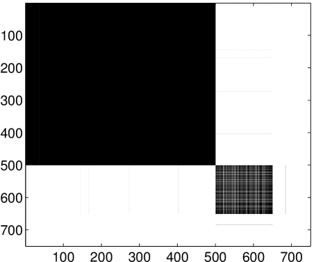
Figure 2: The solution to (CP1) with mid-size clusters.

5 Discussion

An immediate future research is to better understand the “mid-size crisis”. Our current results say nothing about clusters that are neither big nor small, falling in the interval $(\ell_{\flat},\ell_{\sharp})$. Our numerical experiments confirm that the mid-size phenomenon is real: they are neither completely recovered nor entirely ignored by the optimal $\hat{K}$. The part of $\hat{K}$ restricted to these clusters does not seem to have an obvious pattern.Proving whether we can still efficiently recover large clusters in the presence of mid-size clusters is an interesting open problem.

Our study was mainly theoretical, focusing on the planted partition model. As such, our experiments focused on confirming the theoretical findings with data generated exactly according to the distribution we could provide provable guarantees for. It would be interesting to apply the presented methodology to real applications, particularly big data sets merged from web application and social networks.

Another interesting direction is extending the “peeling strategy” to other high-dimensional learning problems. This requires understanding when such a strategy may work. One intuitive explanation of the small cluster barrier encountered in previous work is ambiguity – when viewing the input at the “big cluster resolution”, a small cluster is both a low-rank matrix and a sparse matrix. Only when “zooming in” (after recovering big clusters), small clusters patterns emerge. There are other formulations with similar property. For example, in Xu et al. (2012), the authors propose to decompose a matrix into the sum of a low rank one and a column sparse one to solve an outlier-resistant PCA task. Notice that a column sparse matrix is also a low rank matrix. We hope the “peeling strategy” may also help with that problem.

Appendix A Notation and Conventions

We use the following notation and conventions throughout the supplement. For a real $n\times n$ matrix $M$, we use the unadorned norm $\|M\|$ to denote its spectral norm. The notation $\|M\|_{F}$ refers to the Frobenius norm, $\|M\|_{1}$ is $\sum_{i,j}|M(i,j)|$ and $\|M\|_{\infty}$ is $\max_{ij}|M(i,j)|$.

We will also study operators on the space of matrices. To distinguish them from the matrices studied in this work, we will simply call these objects “operators”, and will denote them using a calligraphic font, e.g. $\mathcal{P}$. The norm $\|\mathcal{P}\|$ of an operator is defined as

$$\|\mathcal{P}\|=\sup_{M:\|M\|_{F}=1}\|\mathcal{P}M\|_{F}\ ,$$

where the supremum is over matrices $M$.

For a fixed, real $n\times n$ matrix $M$, we define the matrix linear subspace $T(M)$ as follows:

$$T(M):=\{YM+MX:X,Y\in\mathbb{R}^{n\times n}\}\ .$$

In words, this subspace is the set of matrices spanned by matrices each row of which is in the row space of $M$, and matrices each column of which is in the column space of $M$.

For any given subspace of matrices $S\subseteq\mathbb{R}^{n\times n}$, we let $\mathcal{P}_{S}$ denote the orthogonal projection onto $S$ with respect to the the inner product $\langle X,Y\rangle=\sum_{i,j=1}^{n}X(i,j)Y(i,j)=\operatorname{tr}X^{t}Y$. This means that for any matrix $M$,

$$\mathcal{P}_{S}M=\operatorname{argmin}_{X\in S}\|M-X\|_{F}\ .$$

For a matrix $M$, we let $\Gamma(M)$ denote the set of matrices supported on a subset of the support of $M$. Note that for any matrix $X$,

$$(\mathcal{P}_{\Gamma(X)}M)(i,j)=\begin{cases}M(i,j)&X(i,j)\neq 0\\ 0&\mbox{otherwise}\end{cases}.$$

It is a well known fact that $\mathcal{P}_{T(X)}$ is given as follows:

$$\mathcal{P}_{T(X)}M=P_{C(X)}M+MP_{R(X)}-P_{C(X)}MP_{R(X)}\ ,$$

where $P_{C(X)}$ is projection (of a vector) onto the column space of $X$, and $P_{R(X)}$ is projection onto the row space of $X$.

For a subspace $S\subseteq\mathbb{R}^{n\times n}$ we let $S^{\perp}$ denote the orthogonal subspace with respect to $\langle\cdot,\cdot\rangle$:

$$S^{\perp}=\{X\in\mathbb{R}^{n\times n}:\langle X,Y\rangle=0\ \forall Y\in S\}\ .$$

Slightly abusing notation, we will use the set complement operator $(\cdot)^{c}$ to formally define $\Gamma(M)^{c}$ to be $\Gamma(M)^{\perp}$ (by this we are stressing that the space $\Gamma(M)^{\perp}$ is given as $\Gamma(M^{\prime})$ where $M^{\prime}$ is any matrix such that $M$ and $M^{\prime}$ have complementary supports). Note that $\mathcal{P}_{T(X)^{\perp}}M=M-\mathcal{P}_{T(X)}M=(I-P_{C(X)})M(I-P_{R(X)})\ .$

For a matrix $M$, $\operatorname{sgn}M$ is defined as the matrix satisfying:

$$(\operatorname{sgn}M)(i,j)=\begin{cases}1&M(i,j)>0\\ -1&M(i,j)<0\\ 0&\mbox{otherwise}\end{cases}\ .$$

Appendix B Proof of Theorem 1

The proof is based on Chen et al. [2012]. We prove it for $\kappa=1$. The adjustment for $\kappa>1$ is done using a padding argument, presented at the end of the proof.

Additional notation:

1. We let $V_{\flat}\subseteq V$ denote the set of of elements $i$ such that $n_{\langle i\rangle}\leq\ell_{\flat}$. (We remind the reader that $n_{\langle i\rangle}=|V_{\langle i\rangle}|$.)

2. We remind the reader that the projection ${\mathcal{P}}_{\sharp}$ is defined as follows:

   $$({\mathcal{P}}_{\sharp}M)(i,j)=\begin{cases}M(i,j)&\max\{n_{\langle i\rangle},n_{\langle j\rangle}\}\geq\ell_{\sharp}\\ 0&\mbox{otherwise}\end{cases}\ .$$

3. The projection ${\mathcal{P}}_{\flat}$ is defined as follows:

   $$({\mathcal{P}}_{\flat}M)(i,j)=\begin{cases}M(i,j)&\max\{n_{\langle i\rangle},n_{\langle j\rangle}\}\leq\ell_{\flat}\\ 0&\mbox{otherwise}\end{cases}\ .$$

   In words, ${\mathcal{P}}_{\flat}$ projects onto the set of matrices supported on $V_{\flat}\times V_{\flat}$. Note that by the theorem assumption, ${\mathcal{P}}_{\sharp}+{\mathcal{P}}_{\flat}={\mathcal{I}d}$ (equivalently, ${\mathcal{P}}_{\sharp}$ projects onto the set of matrices supported on $(V\times V)\setminus(V_{\flat}\times V_{\flat})$).

4. Define the set

   $$\mathfrak{D}=\left\{\Delta\in\mathbb{R}^{n\times n}|\Delta_{ij}\leq 0,\forall i\sim j,(i,j)\notin V_{\flat}\times V_{\flat};0\leq\Delta_{ij},\forall i\not\sim j,(i,j)\notin V_{\flat}\times V_{\flat}\right\},$$

   which contains all feasible deviation from $\hat{K}$.

5. For simplicity we write $T:=T(\hat{K})$ and $\Gamma:=\Gamma(\hat{B}),\Gamma^{c}:=\Gamma(\hat{B})^{c}=\Gamma^{\perp}$.

We will make use of the following:

1. $\operatorname{sgn}(\hat{B})=\hat{B}$.

2. ${\mathcal{I}d}=\mathcal{P}_{\Gamma}+\mathcal{P}_{\Gamma^{c}}=\mathcal{P}_{\Gamma(A)}+\mathcal{P}_{\Gamma(A)^{c}}$.

3. ${\mathcal{P}}_{\sharp},{\mathcal{P}}_{\flat},\mathcal{P}_{\Gamma},\mathcal{P}_{\Gamma^{c}},\mathcal{P}_{\Gamma(A)},$ and $\mathcal{P}_{\Gamma(A)^{c}}$ commute with each other.

B.1 Approximate Dual Certificate Condition

Proposition 12.

$(\hat{K}$, $\hat{B}$) is the unique optimal solution to (CP) if there exists a matrix $Q\in\mbox{$\mathbb{R}$}^{n\times n}$ and a positive number $\epsilon$ satisfying:

1. $\left\|Q\right\|<1$

2. $\left\|\mathcal{P}_{T}(Q)\right\|_{\infty}\leq\frac{\epsilon}{2}\min\left\{c_{1},c_{2}\right\}$

3. $\forall\Delta\in\mathfrak{D}$:

   1. $\left\langle UU^{\top}+Q,\mathcal{P}_{\Gamma(A)}\mathcal{P}_{\Gamma}{\mathcal{P}}_{\sharp}\Delta\right\rangle=(1+\epsilon)c_{1}\left\|\mathcal{P}_{\Gamma(A)}P_{\Gamma}{\mathcal{P}}_{\sharp}\Delta\right\|_{1}$

   2. $\left\langle UU^{\top}+Q,\mathcal{P}_{\Gamma(A)^{c}}\mathcal{P}_{\Gamma}{\mathcal{P}}_{\sharp}\Delta\right\rangle=(1+\epsilon)c_{2}\left\|\mathcal{P}_{\Gamma(A)^{c}}P_{\Gamma}{\mathcal{P}}_{\sharp}\Delta\right\|_{1}$

4. $\forall\Delta\in\mathfrak{D}$:

   1. $\left\langle UU^{\top}+Q,\mathcal{P}_{\Gamma(A)}\mathcal{P}_{\Gamma^{c}}\mathcal{P}_{\sharp}\Delta\right\rangle\geq-(1-\epsilon)c_{1}\left\|\mathcal{P}_{\Gamma(A)}P_{\Gamma^{c}}{\mathcal{P}}_{\sharp}\Delta\right\|_{1}$

   2. $\left\langle UU^{\top}+Q,\mathcal{P}_{\Gamma(A)^{c}}\mathcal{P}_{\Gamma^{c}}\mathcal{P}_{\sharp}\Delta\right\rangle\geq-(1-\epsilon)c_{2}\left\|\mathcal{P}_{\Gamma(A)^{c}}P_{\Gamma^{c}}{\mathcal{P}}_{\sharp}\Delta\right\|_{1}$

5. $\mathcal{P}_{\Gamma}{\mathcal{P}}_{\flat}(UU^{\top}+Q)=c_{1}{\mathcal{P}}_{\flat}\hat{B}$

6. $\left\|\mathcal{P}_{\Gamma^{c}}{\mathcal{P}}_{\flat}(UU^{\top}+Q)\right\|_{\infty}\leq c_{2}$

Proof.

Consider any feasible solution to (CP1) $(\hat{K}+\Delta,\hat{B}-\Delta)$; we know $\Delta\in\mathfrak{D}$ due to the inequality constraints in (CP1). We will show that this solution will have strictly higher objective value than $\left\langle\hat{K},\hat{B}\right\rangle$ if $\Delta\neq 0$.

For this $\Delta$, let $G_{\Delta}$ be a matrix in $T^{\bot}\cap\mbox{Range}({\mathcal{P}}_{\flat})$ satisfying $\left\|G\right\|=1$ and $\left\langle G_{\Delta},\Delta\right\rangle=\left\|\mathcal{P}_{T^{\bot}}{\mathcal{P}}_{\flat}\Delta\right\|_{*}$ ; such a matrix always exists because $\mbox{Range}{\mathcal{P}}_{\flat}\subseteq T^{\bot}$. Suppose $\left\|Q\right\|=b$. Clearly, $\mathcal{P}_{T^{\bot}}Q+(1-b)G\in T^{\bot}$ and, due to desideratum 1, we have $\left\|\mathcal{P}_{T^{\bot}}Q+(1-b)G_{\Delta}\right\|\leq\left\|Q\right\|+(1-b)\left\|G_{\Delta}\right\|=b+(1-b)=1$. Therefore, $UU^{\top}+\mathcal{P}_{T^{\bot}}Q+(1-b)G_{\Delta}$ is a subgradient of $f(K)=\left\|K\right\|_{*}$ at $K=\hat{K}$. On the other hand, define the matrix $F_{\Delta}=-\mathcal{P}_{\Gamma^{c}}\mbox{sgn}(\Delta)$. We have $F_{\Delta}\in\Gamma^{c}$ and $\left\|F_{\Delta}\right\|_{\infty}\leq 1$. Therefore, $\mathcal{P}_{\Gamma(A)}(\hat{B}+F_{\Delta})$ is a subgradient of $g_{1}(B)=\left\|\mathcal{P}_{\Gamma(A)}B\right\|_{1}$ at $B=\hat{B}$, and $\mathcal{P}_{\Gamma(A)^{c}}(\hat{B}+F_{\Delta})$ is a subgradient of $g_{2}(B)=\left\|\mathcal{P}_{\Gamma(A)^{c}}B\right\|_{1}$ at $B=\hat{B}$. Using these three subgradients, the difference in the objective value can be bounded as follows:

$$d(\Delta)$$

$$\triangleq \left\|\hat{K}+\Delta\right\|_{*}+c_{1}\left\|\mathcal{P}_{\Gamma(A)}(\hat{B}-\Delta)\right\|_{1}+c_{2}\left\|\mathcal{P}_{\Gamma(A)^{c}}(\hat{B}-\Delta)\right\|_{1}-\left\|\hat{K}\right\|_{*}-c_{1}\left\|\mathcal{P}_{\Gamma(A)}\hat{B}\right\|_{1}-c_{2}\left\|\mathcal{P}_{\Gamma(A)^{c}}\hat{B}\right\|_{1}$$

$$\geq \left\langle UU^{\top}+\mathcal{P}_{T^{\bot}}Q+(1-b)G_{\Delta},\Delta\right\rangle+c_{1}\left\langle\mathcal{P}_{\Gamma(A)}(\hat{B}+F_{\Delta}),-\Delta\right\rangle+c_{2}\left\langle\mathcal{P}_{\Gamma(A)^{c}}(\hat{B}+F_{\Delta}),-\Delta\right\rangle$$

$$= (1-b)\left\|\mathcal{P}_{T^{\bot}}{\mathcal{P}}_{\flat}\Delta\right\|_{*}+\left\langle UU^{\top}+\mathcal{P}_{T^{\bot}}Q,\Delta\right\rangle+c_{1}\left\langle\mathcal{P}_{\Gamma(A)}\hat{B},-\Delta\right\rangle+c_{2}\left\langle\mathcal{P}_{\Gamma(A)^{c}}\hat{B},-\Delta\right\rangle$$

$$+c_{1}\left\langle\mathcal{P}_{\Gamma(A)}F_{\Delta},-\Delta\right\rangle+c_{2}\left\langle\mathcal{P}_{\Gamma(A)^{c}}F_{\Delta},-\Delta\right\rangle$$

$$= (1-b)\left\|\mathcal{P}_{T^{\bot}}{\mathcal{P}}_{\flat}\Delta\right\|_{*}+\left\langle UU^{\top}+\mathcal{P}_{T^{\bot}}Q,\Delta\right\rangle+c_{1}\left\langle{\mathcal{P}}_{\flat}\mathcal{P}_{\Gamma(A)}\hat{B},-\Delta\right\rangle+c_{2}\left\langle{\mathcal{P}}_{\flat}\mathcal{P}_{\Gamma(A)^{c}}\hat{B},-\Delta\right\rangle$$

$$+c_{1}\left\langle{\mathcal{P}}_{\sharp}\mathcal{P}_{\Gamma(A)}\hat{B},-\Delta\right\rangle+c_{2}\left\langle{\mathcal{P}}_{\sharp}\mathcal{P}_{\Gamma(A)^{c}}\hat{B},-\Delta\right\rangle+c_{1}\left\langle\mathcal{P}_{\Gamma(A)}F_{\Delta},-\Delta\right\rangle+c_{2}\left\langle\mathcal{P}_{\Gamma(A)^{c}}F_{\Delta},-\Delta\right\rangle.$$

The last six terms of the last RHS satisfy:

1. $c_{1}\left\langle{\mathcal{P}}_{\flat}\mathcal{P}_{\Gamma(A)}\hat{B},-\Delta\right\rangle+c_{2}\left\langle{\mathcal{P}}_{\flat}\mathcal{P}_{\Gamma(A)^{c}}\hat{B},-\Delta\right\rangle=c_{1}\left\langle{\mathcal{P}}_{\flat}\hat{B},-\Delta\right\rangle$, because ${\mathcal{P}}_{\flat}\hat{B}\in\Gamma(A)$.

2. $\left\langle{\mathcal{P}}_{\sharp}\mathcal{P}_{\Gamma(A)}\hat{B},-\Delta\right\rangle\geq-\left\|{\mathcal{P}}_{\sharp}\mathcal{P}_{\Gamma(A)}\mathcal{P}_{\Gamma}\Delta\right\|_{1}$ and $\left\langle{\mathcal{P}}_{\sharp}\mathcal{P}_{\Gamma(A)^{c}}\hat{B},\Delta\right\rangle\geq-\left\|{\mathcal{P}}_{\sharp}\mathcal{P}_{\Gamma(A)^{c}}\mathcal{P}_{\Gamma}\Delta\right\|_{1}$, because $\hat{B}\in\Gamma$ and$\left\|\hat{B}\right\|_{\infty}\leq 1$.

3. $\left\langle\mathcal{P}_{\Gamma(A)}F_{\Delta},-\Delta\right\rangle=\left\|\mathcal{P}_{\Gamma(A)}\mathcal{P}_{\Gamma^{c}}\Delta\right\|_{1}$ and $\left\langle\mathcal{P}_{\Gamma(A)^{c}}F_{\Delta},-\Delta\right\rangle=\left\|\mathcal{P}_{\Gamma(A)^{c}}\mathcal{P}_{\Gamma^{c}}\Delta\right\|_{1}$, due to the definition of $F$.

It follows that

$$d(\Delta) \geq (1-b)\left\|\mathcal{P}_{T^{\bot}}{\mathcal{P}}_{\flat}\Delta\right\|_{*}+\left\langle UU^{\top}+\mathcal{P}_{T^{\bot}}Q,\Delta\right\rangle+c_{1}\left\langle{\mathcal{P}}_{\flat}\hat{B},-\Delta\right\rangle-c_{1}\left\|{\mathcal{P}}_{\sharp}\mathcal{P}_{\Gamma(A)}\mathcal{P}_{\Gamma}\Delta\right\|_{1}$$ (6)

$$-c_{2}\left\|{\mathcal{P}}_{\sharp}\mathcal{P}_{\Gamma(A)^{c}}\mathcal{P}_{\Gamma}\Delta\right\|_{1}+c_{1}\left\|\mathcal{P}_{\Gamma(A)}\mathcal{P}_{\Gamma^{c}}\Delta\right\|_{1}+c_{2}\left\|\mathcal{P}_{\Gamma(A)^{c}}\mathcal{P}_{\Gamma^{c}}\Delta\right\|_{1}.$$

Consider the second term in the last RHS, which equals $\left\langle UU^{\top}+\mathcal{P}_{T^{\bot}}Q,\Delta\right\rangle=\left\langle UU^{\top}+Q,{\mathcal{P}}_{\sharp}\Delta\right\rangle+\left\langle UU^{\top}+Q,{\mathcal{P}}_{\flat}\Delta\right\rangle-\left\langle\mathcal{P}_{T}Q,\Delta\right\rangle$. We bound these three separately.

First term:

$$\left\langle UU^{\top}+Q,{\mathcal{P}}_{\sharp}\Delta\right\rangle$$

$$= \left\langle UU^{\top}+Q,\left(\mathcal{P}_{\Gamma(A)}\mathcal{P}_{\Gamma}{\mathcal{P}}_{\sharp}+\mathcal{P}_{\Gamma(A)^{c}}\mathcal{P}_{\Gamma}{\mathcal{P}}_{\sharp}+\mathcal{P}_{\Gamma(A)}\mathcal{P}_{\Gamma^{c}}{\mathcal{P}}_{\sharp}+\mathcal{P}_{\Gamma(A)^{c}}\mathcal{P}_{\Gamma^{c}}{\mathcal{P}}_{\sharp}\right)\Delta\right\rangle$$

$$\geq (1+\epsilon)c_{1}\left\|\mathcal{P}_{\Gamma(A)}P_{\Gamma}{\mathcal{P}}_{\sharp}\Delta\right\|_{1}+(1+\epsilon)c_{2}\left\|\mathcal{P}_{\Gamma(A)^{c}}P_{\Gamma}{\mathcal{P}}_{\sharp}\Delta\right\|_{1}-(1-\epsilon)c_{1}\left\|\mathcal{P}_{\Gamma(A)}P_{\Gamma^{c}}{\mathcal{P}}_{\sharp}\Delta\right\|_{1}$$

$$-(1-\epsilon)c_{2}\left\|\mathcal{P}_{\Gamma(A)^{c}}P_{\Gamma^{c}}{\mathcal{P}}_{\sharp}\Delta\right\|_{1}$$

(Using properties 3 and 4)

Second term:

$$\left\langle UU^{\top}+Q,{\mathcal{P}}_{\flat}\Delta\right\rangle$$

$$= \left\langle\mathcal{P}_{\Gamma}{\mathcal{P}}_{\flat}(UU^{\top}+Q),\Delta\right\rangle+\left\langle\mathcal{P}_{\Gamma^{c}}{\mathcal{P}}_{\flat}(UU^{\top}+Q),\Delta\right\rangle$$

$$\geq c_{1}\left\langle{\mathcal{P}}_{\flat}\hat{B},\Delta\right\rangle-c_{2}\left\|\mathcal{P}_{\Gamma^{c}}{\mathcal{P}}_{\flat}\Delta\right\|_{1}\mbox{ (using properties 5 and 6)}$$

$$= c_{1}\left\langle{\mathcal{P}}_{\flat}\hat{B},\Delta\right\rangle-c_{2}\left\|\mathcal{P}_{\Gamma(A)^{c}}\mathcal{P}_{\Gamma^{c}}{\mathcal{P}}_{\flat}\Delta\right\|_{1}\mbox{ (because $\mathcal{P}_{\Gamma(A)^{c}}\mathcal{P}_{\Gamma^{c}}{\mathcal{P}}_{\flat}=\mathcal{P}_{\Gamma^{c}}{\mathcal{P}}_{\flat}$)}$$

Third term: Due to the block diagonal structure of the elements of $T$, we have $\mathcal{P}_{T}={\mathcal{P}}_{\sharp}\mathcal{P}_{T}$

$$\left\langle-\mathcal{P}_{T}Q,\Delta\right\rangle$$

$$= -\left\langle\mathcal{P}_{T}Q,{\mathcal{P}}_{\sharp}\Delta\right\rangle$$

$$\geq -\left\|\mathcal{P}_{T}Q\right\|_{\infty}\left\|{\mathcal{P}}_{\sharp}\Delta\right\|_{1}$$

$$\geq -\frac{\epsilon}{2}\min\left\{c_{1},c_{2}\right\}\left\|{\mathcal{P}}_{\sharp}\Delta\right\|_{1}.$$

Combining the above three bounds with Eq. (6), we obtain

$$d(\Delta)$$

$$\geq (1-b)\left\|\mathcal{P}_{T^{\bot}}{\mathcal{P}}_{\flat}\Delta\right\|_{*}+\epsilon c_{1}\left\|{\mathcal{P}}_{\sharp}\mathcal{P}_{\Gamma(A)}\mathcal{P}_{\Gamma}\Delta\right\|_{1}+\epsilon c_{2}\left\|{\mathcal{P}}_{\sharp}\mathcal{P}_{\Gamma(A)^{c}}\mathcal{P}_{\Gamma}\Delta\right\|_{1}+\epsilon c_{1}\left\|\mathcal{P}_{\Gamma(A)}\mathcal{P}_{\Gamma^{c}}{\mathcal{P}}_{\sharp}\Delta\right\|_{1}$$

$$+\epsilon c_{2}\left\|\mathcal{P}_{\Gamma(A)^{c}}\mathcal{P}_{\Gamma^{c}}{\mathcal{P}}_{\sharp}\Delta\right\|_{1}+c_{1}\left\|\mathcal{P}_{\Gamma(A)}\mathcal{P}_{\Gamma^{c}}{\mathcal{P}}_{\flat}\Delta\right\|_{1}-\frac{\epsilon}{2}\min\left\{c_{1},c_{2}\right\}\left\|{\mathcal{P}}_{\sharp}\Delta\right\|_{1}$$

$$= (1-b)\left\|\mathcal{P}_{T^{\bot}}{\mathcal{P}}_{\flat}\Delta\right\|_{*}+\epsilon c_{1}\left\|{\mathcal{P}}_{\sharp}\mathcal{P}_{\Gamma(A)}\Delta\right\|_{1}+\epsilon c_{2}\left\|{\mathcal{P}}_{\sharp}\mathcal{P}_{\Gamma(A)^{c}}\Delta\right\|_{1}-\frac{\epsilon}{2}\min\left\{c_{1},c_{2}\right\}\left\|{\mathcal{P}}_{\sharp}\Delta\right\|_{1}$$

(note that $$\mathcal{P}_{\Gamma(A)}\mathcal{P}_{\Gamma^{c}}{\mathcal{P}}_{\flat}\Delta$$=0)

$$\geq (1-b)\left\|{\mathcal{P}}_{\flat}\Delta\right\|_{*}+\frac{\epsilon}{2}\min\left\{c_{1},c_{2}\right\}\left\|{\mathcal{P}}_{\sharp}\Delta\right\|_{1},$$

which is strictly greater than zero for $\Delta\neq 0$. ∎

B.2 Constructing $Q$.

We construct a matrix $Q$ with the properties required by Proposition 12. Suppose we take $\epsilon=\frac{2\log^{2}n}{\ell_{\sharp}}\sqrt{\frac{n}{t(1-t)}}$ and use the weights $c_{1}$ and $c_{2}$ given in Theorem 1. We specify ${\mathcal{P}}_{\sharp}Q$ and ${\mathcal{P}}_{\flat}Q$ separately.

${\mathcal{P}}_{\sharp}Q$ is given by ${\mathcal{P}}_{\sharp}Q={\mathcal{P}}_{\sharp}Q_{1}+{\mathcal{P}}_{\sharp}Q_{2}+{\mathcal{P}}_{\sharp}Q_{3}$, where for $(i,j)\notin V_{\flat}\times V_{\flat}$,

$${\mathcal{P}}_{\sharp}Q_{1}(i,j) = \begin{cases}-\frac{1}{n_{c(i)}}&i\sim j,(i,j)\in\Gamma\\ \frac{1}{n_{c(i)}}\cdot\frac{1-p_{ij}}{p_{ij}}&i\sim j,(i,j)\in\Gamma^{c}\\ 0&i\not\sim j\end{cases}$$

$${\mathcal{P}}_{\sharp}Q_{2}(i,j) = \begin{cases}-(1+\epsilon)c_{2}&i\sim j,(i,j)\in\Gamma\\ (1+\epsilon)c_{2}\frac{1-p_{ij}}{p_{ij}}&i\sim j,(i,j)\in\Gamma^{c}\\ 0&i\not\sim j\end{cases}$$

$${\mathcal{P}}_{\sharp}Q_{3}(i,j) = \begin{cases}(1+\epsilon)c_{1}&i\not\sim j,(i,j)\in\Gamma\\ -(1+\epsilon)c_{1}\frac{q_{ij}}{1-q_{ij}}&i\not\sim j,(i,j)\in\Gamma^{c}\\ 0&i\sim,j\end{cases}$$

Note that these matrices have zero-mean entries.

${\mathcal{P}}_{\flat}Q$ as follows. For $(i,j)\in V_{\flat}\times V_{\flat}$,

$${\mathcal{P}}_{\flat}Q=\begin{cases}c_{1}&i\sim j,(i,j)\in\Gamma(A)\\ -c_{2}&i\sim j,(i,j)\in\Gamma(A)^{c}\\ c_{1}&i\not\sim j,(i,j)\in\Gamma(A)\\ c_{2}W(i,j)&i\not\sim j,(i,j)\in\Gamma(A)^{c}\end{cases},$$

where

$$W(i,j)=\begin{cases}+1&\mbox{with probability $\frac{t-q}{2t(1-q)}$}\\ -1&\mbox{with remaining probability}\end{cases}.$$

B.3 Validating $Q$

Under the choice of $t$ in Theorem 1, we have $\frac{1}{4}p\leq t\leq p$ and $\frac{1}{4}(1-q)\leq 1-t\leq 1-q$. Also under the second assumption of the theorem and $p-q\leq p(1-q)$, we have $p(1-q)\gtrsim\frac{n\log^{4}n}{\ell_{\sharp}^{2}}\geq\frac{\log^{4}n}{\ell_{\sharp}}$. We will make use of these facts frequently in the proof.

It is easy to check that $\epsilon:=\frac{2\log^{2}n}{\ell_{\sharp}}\sqrt{\frac{n}{t(1-t)}}<\frac{1}{2}$ under the assumption of Theorem 1.

Property 1):

Note that $\left\|Q\right\|\leq\left\|{\mathcal{P}}_{\sharp}Q_{\sim}\right\|+\left\|{\mathcal{P}}_{\sharp}Q_{\not\sim}\right\|+\left\|{\mathcal{P}}_{\flat}Q_{\sim}\right\|+\left\|{\mathcal{P}}_{\flat}Q_{\not\sim}\right\|$. We show that all four terms are upper-bounded by $\frac{1}{4}$.

(a) ${\mathcal{P}}_{\flat}Q_{\sim}$ is a block diagonal matrix with each block having size at most $\ell_{\flat}$. Moreover, ${\mathcal{P}}_{\flat}Q_{\sim}$ is the sum of a deterministic matrix $Q_{\sim,d}$ with all non-zero entries equal to $\frac{b_{1}}{\sqrt{n\log n}}\frac{p-t}{\sqrt{t(1-t)}}$ and a random matrix $Q_{\sim,r}$ whose entries are i.i.d., bounded almost surely by $\max\{c_{1},c_{2}\}$ and have zero mean with variance $\frac{b_{1}^{2}}{n\log n}\cdot\frac{p(1-p)}{t(1-t)}$. Therefore, we have $\|Q_{\sim}\|\leq\|Q_{\sim,r}\|+\|Q_{\sim,d}\|$, where w.h.p.

$$\left\|{\mathcal{P}}_{\flat}Q_{\sim,d}\right\| \leq \ell_{\flat}\frac{b_{1}}{\sqrt{n\log n}}\frac{p-t}{\sqrt{t(1-t)}},$$

$$\left\|{\mathcal{P}}_{\flat}Q_{\sim,r}\right\| \leq 6\max\left\{\sqrt{\ell_{\flat}\log n}\frac{b_{1}}{\sqrt{n\log n}}\sqrt{\frac{p(1-p)}{t(1-t)}}+\max\{c_{1},c_{2}\}\log^{2}n\right\};$$

here in the second inequality we use Lemma 16. We conclude that $\left\|{\mathcal{P}}_{\flat}Q_{\sim}\right\|$ is bounded by $\frac{1}{4}$ as long as $\ell_{\flat}\leq\frac{\sqrt{t(1-t)n\log n}}{8b_{1}(p-t)}$ and $\max\{c_{1},c_{2}\}\leq\frac{1}{48\log^{2}n}$, which holds under the assumption of Theorem 1.

(b) ${\mathcal{P}}_{\flat}Q_{\not\sim}$ is a random matrix supported on $V_{\flat}\times V_{\flat}$, whose entries are i.i.d., zero mean, bounded almost surely by $\max\{c_{1},c_{2}\}$, and have variance $\frac{b_{1}^{2}}{n\log n}\cdot\frac{t^{2}+q-2tq}{(1-t)t}$. It follows from Lemma 16 that

$$\left\|{\mathcal{P}}_{\flat}Q_{\not\sim}\right\|\leq 6\max\left\{\sqrt{n_{\flat}}\cdot\frac{b_{1}}{\sqrt{n\log n}}\sqrt{\frac{t^{2}+q-2tq}{(1-t)t}},\max\{c_{1},c_{2}\}\log^{2}n\right\}\leq\frac{1}{4}$$

because $n_{\flat}\leq n$ and $\max\{c_{1},c_{2}\}\leq\frac{1}{48\log^{2}n}$, which holds under the assumption of the theorem.

(c) Note that ${\mathcal{P}}_{\sharp}Q_{\sim}={\mathcal{P}}_{\sharp}Q_{1}+{\mathcal{P}}_{\sharp}Q_{2}$. By construction these two matrices are both block-diagonal, have i.i.d zero-mean entries which are bounded almost surely by $B_{\sim}:=\max\left\{\frac{1}{\ell_{\sharp}p},\frac{2c_{2}}{p}\right\}$ and have variance bounded by $\sigma_{\sim}^{2}:=\max\left\{\frac{1-p}{p\ell_{\sharp}^{2}},\frac{4(1-p)}{p}c_{2}^{2}\right\}$. Lemma 16 gives $\left\|{\mathcal{P}}_{\sharp}Q_{\sim}\right\|\leq 6\max\left\{\sqrt{\ell_{\sharp}}\cdot\sigma_{\sim},B_{\sim}\log^{2}n\right\}\leq\frac{1}{4}$ under the assumption of Theorem 1.

(d) Note that ${\mathcal{P}}_{\sharp}Q_{\not\sim}={\mathcal{P}}_{\sharp}Q_{3}$ is a random matrix with i.i.d. zero-mean entries which are bounded almost surely by $B_{\not\sim}:=\frac{2c_{1}}{1-q}$ and have variance bounded by $\sigma_{\not\sim}^{2}:=\frac{4q}{1-q}c_{1}^{2}$. Lemma 16 gives $\left\|{\mathcal{P}}_{\sharp}Q_{\not\sim}\right\|\leq 6\max\left\{\sqrt{n}\cdot\sigma_{\not\sim},B_{\not\sim}\log^{2}n\right\}\leq\frac{1}{4}$.

Property 2):

Due to the structure of $T$, we have

$$\left\|\mathcal{P}_{T}Q\right\|_{\infty} = \left\|\mathcal{P}_{T}{\mathcal{P}}_{\sharp}Q\right\|_{\infty}=\left\|UU^{\top}({\mathcal{P}}_{\sharp}Q)+({\mathcal{P}}_{\sharp}Q)UU^{\top}+UU^{\top}({\mathcal{P}}_{\sharp}Q)UU^{\top}\right\|_{\infty}$$

$$\leq 3\left\|UU^{\top}{\mathcal{P}}_{\sharp}Q\right\|_{\infty}\leq 3\sum_{m=1}^{3}\left\|UU^{\top}{\mathcal{P}}_{\sharp}Q_{m}\right\|_{\infty}.$$

Now observe that $(UU^{\top}{\mathcal{P}}_{\sharp}Q_{m})(i,j)=\sum_{l\in V_{c(i)}}\frac{1}{n_{c(i)}}{\mathcal{P}}_{\sharp}Q_{m}(l,j)$ is the sum of i.i.d. zero-mean random variables with bounded magnitude and variance. Using Lemma 18, we obtain that for $i\in V_{\sharp}$,

$$\left|(UU^{\top}{\mathcal{P}}_{\sharp}Q_{1})(i,j)\right| \lesssim \frac{1}{n_{c(i)}}\left(\sqrt{\frac{1-p}{p\ell_{\sharp}^{2}}}\cdot\sqrt{n_{c(i)}\log n}+\frac{\log n}{\ell_{\sharp}p}\right)$$

$$\leq \frac{1}{\ell_{\sharp}}\sqrt{\frac{\log n}{p\ell_{\sharp}}}\leq\frac{\log n}{24^{2}\ell_{\sharp}}\sqrt{\frac{t}{p}}.$$

where in the last inequality we use $t\geq\frac{p}{4}\gtrsim\frac{\log n}{\ell_{\sharp}}$. For $i\in V_{\flat}$, clearly $(UU^{\top}{\mathcal{P}}_{\sharp}Q_{1})(i,j)=0$. By union bound we conclude that $\left\|UU^{\top}{\mathcal{P}}_{\sharp}Q_{1}\right\|_{\infty}\leq\frac{\log n}{24^{2}\ell_{\sharp}}\sqrt{\frac{t}{p}}.$ Similarly, we can bound $\left\|UU^{\top}{\mathcal{P}}_{\sharp}Q_{2}\right\|_{\infty}$ and $\left\|UU^{\top}{\mathcal{P}}_{\sharp}Q_{3}\right\|_{\infty}$ with the same quantity (cf. Chen et al. [2012]).

On the other hand, under the definition of $c_{1},c_{2}$ and $\epsilon$, we have

$$c_{1}\epsilon=b_{1}\sqrt{\frac{1-t}{tn\log n}}\cdot\frac{2\log^{2}n}{\ell_{\sharp}}\sqrt{\frac{n}{t(1-t)}}=b_{1}\frac{\sqrt{p\log n}}{t\sqrt{t}}\cdot\frac{\log n}{24\ell_{\sharp}}\sqrt{\frac{t}{p}}\geq\frac{\log n}{24\ell_{\sharp}}\sqrt{\frac{t}{p}}$$

and similarly $c_{2}\epsilon\geq\frac{\log n}{24\ell_{\sharp}}\sqrt{\frac{t}{p}}$. It follows that $\left\|\mathcal{P}_{T}Q\right\|_{\infty}\leq 9\cdot\frac{1}{24}\epsilon\min\left\{c_{1},c_{2}\right\}$, proving property 2).

Properties 3a) and 3b)

For 3a), by construction of $Q$ we have

$$\left\langle UU^{\top}+Q,\mathcal{P}_{\Gamma(A)}\mathcal{P}_{\Gamma}{\mathcal{P}}_{\sharp}\Delta\right\rangle = \left\langle\mathcal{P}_{\Gamma(A)}\mathcal{P}_{\Gamma}{\mathcal{P}}_{\sharp}Q_{3},\mathcal{P}_{\Gamma(A)}\mathcal{P}_{\Gamma}{\mathcal{P}}_{\sharp}\Delta\right\rangle$$

$$= (1+\epsilon)c_{1}\sum_{(i,j)\in\Gamma\cap\Gamma(A)}{\mathcal{P}}_{\sharp}\Delta(i,j)$$

$$= (1+\epsilon)c_{1}\left\|\mathcal{P}_{\Gamma(A)}\mathcal{P}_{\Gamma}{\mathcal{P}}_{\sharp}\Delta\right\|_{1}\mbox{ (because $\Delta\in\mathfrak{D}$)}$$

Property 3b) can be verified similarly.

Properties 4a) and 4b):

For 4a), we have

$$\left\langle UU^{\top}+Q,\mathcal{P}_{\Gamma(A)}\mathcal{P}_{\Gamma^{c}}\mathcal{P}_{\sharp}\Delta\right\rangle = \left\langle\mathcal{P}_{\Gamma(A)}\mathcal{P}_{\Gamma^{c}}\mathcal{P}_{\sharp}\left(UU^{\top}+{\mathcal{P}}_{\sharp}Q_{1}+{\mathcal{P}}_{\sharp}Q_{2}\right),\mathcal{P}_{\Gamma(A)}\mathcal{P}_{\Gamma^{c}}\mathcal{P}_{\sharp}\Delta\right\rangle$$

$$= \sum_{(i,j)\in\Gamma^{c}\cap\Gamma(A)}\left(\frac{1}{n_{c(i)}}+\frac{1}{n_{c(i)}}\frac{1-p_{ij}}{p_{ij}}+(1+\epsilon)c_{2}\frac{1-p_{ij}}{p_{ij}}\right)\mathcal{P}_{\sharp}\Delta(i,j)$$

$$\geq -\left(\frac{1}{p\ell_{\sharp}}+(1+\epsilon)c_{2}\frac{1-p}{p}\right)\left\|\mathcal{P}_{\Gamma(A)}P_{\Gamma^{c}}{\mathcal{P}}_{\sharp}\Delta\right\|_{1},$$

$$\mbox{ (here we use $\Delta\in\mathfrak{D}$, $p_{ij}\geq p$, and $n_{c(i)}\geq\ell_{\sharp}$for $i\in V_{\sharp}$)}.$$

Consider the two terms in the parenthesis in the last RHS. For the first term, we have

$$\frac{1}{p\ell_{\sharp}}=\frac{2\log^{2}n}{\ell_{\sharp}}\sqrt{\frac{n}{t(1-t)}}\cdot\sqrt{\frac{t(1-t)}{4p^{2}n\log^{4}n}}\leq\frac{2\log^{2}n}{\ell_{\sharp}}\sqrt{\frac{n}{t(1-t)}}\cdot b_{1}\sqrt{\frac{1-t}{tn\log n}}=\epsilon c_{1}.$$

For the second term, we have the following

$$p-t\geq\frac{p-q}{4} \geq \frac{b_{3}}{4}\frac{\log^{2}n\sqrt{p(1-q)n}}{\ell_{\sharp}}$$

$$= \frac{b_{3}}{4}\cdot\frac{\sqrt{t(1-q})}{\sqrt{p(1-t)}}\cdot p(1-t)\cdot\frac{2\log^{2}n\sqrt{n}}{\ell_{\sharp}\sqrt{t(1-t)}}$$

$$\geq 8\cdot p(1-t)\cdot\frac{2\log^{2}n\sqrt{n}}{\ell_{\sharp}\sqrt{t(1-t)}}=8p(1-t)\epsilon,$$

which implies $(1+\epsilon)c_{2}\frac{1-p}{p}\leq(1-2\epsilon)c_{1}$. We conclude that

$$\left\langle UU^{\top}+Q,\mathcal{P}_{\Gamma(A)}\mathcal{P}_{\Gamma^{c}}\mathcal{P}_{\sharp}\Delta\right\rangle\geq-\left(\epsilon c_{1}+(1-2\epsilon)c_{1}\right)\left\|\mathcal{P}_{\Gamma(A)}P_{\Gamma^{c}}{\mathcal{P}}_{\sharp}\Delta\right\|_{1},$$

proving property 4a).

For 4b), we have

$$\left\langle UU^{\top}+Q,\mathcal{P}_{\Gamma(A)^{c}}\mathcal{P}_{\Gamma^{c}}\mathcal{P}_{\sharp}\Delta\right\rangle = \left\langle\mathcal{P}_{\Gamma(A)^{c}}\mathcal{P}_{\Gamma^{c}}\mathcal{P}_{\sharp}Q_{3},\mathcal{P}_{\Gamma(A)^{c}}\mathcal{P}_{\Gamma^{c}}\mathcal{P}_{\sharp}\Delta\right\rangle$$

$$= \sum_{(i,j)\in\Gamma(A)^{c}\cap\Gamma^{c}\cap\operatorname{Range}{\mathcal{P}}_{\sharp}}-(1+\epsilon)\frac{c_{1}q_{ij}}{1-q_{ij}}{\mathcal{P}}_{\sharp}\Delta(i,j)$$

$$\geq -(1+\epsilon)\frac{c_{1}q}{1-q}\left\|\mathcal{P}_{\Gamma(A)^{c}}\mathcal{P}_{\Gamma^{c}}\mathcal{P}_{\sharp}\Delta\right\|_{1}.\mbox{ (here we use $q_{ij}\leq q$)}$$

Consider the factor before the norm in the last RHS. Similarly as before, we have

$$t-q\geq\frac{p-q}{4} \geq \frac{b_{3}}{4}\frac{\log^{2}n\sqrt{p(1-q)n}}{\ell_{\sharp}}$$

$$\geq 2\cdot t(1-q)\cdot\frac{2\log^{2}n\sqrt{n}}{\ell_{\sharp}\sqrt{t(1-t)}}=2t(1-q)\epsilon.$$

This implies $(1+\epsilon)c_{1}\frac{q}{1-q}\leq(1-\epsilon)c_{2}$. We conclude that

$$\left\langle UU^{\top}+Q,\mathcal{P}_{\Gamma(A)^{c}}\mathcal{P}_{\Gamma^{c}}\mathcal{P}_{\sharp}\Delta\right\rangle\geq-(1-\epsilon)c_{2}\left\|\mathcal{P}_{\Gamma(A)^{c}}\mathcal{P}_{\Gamma^{c}}\mathcal{P}_{\sharp}\Delta\right\|_{1},$$

proving property 4b).

Properties 5) and 6): It is obvious that these two properties hold by construction of $Q$.

Note that properties 3)-6) hold deterministically.

B.4 The $\kappa>1$ case

Let $n^{\prime}=\kappa^{2}n$ and assume $n^{\prime}$ is an integer. Let $A^{\prime}\in\mathbb{R}^{n^{\prime}\times n^{\prime}}$ be such a matrix that

$$A^{\prime}=\left[\begin{array}[]{cc}A&0\\ 0&I\end{array}\right].$$

Consider the following padded program

$$\mbox{(CP1') }\min_{K^{\prime},B^{\prime}\in\mathbb{R}^{n^{\prime}\times n^{\prime}}} \left\|K^{\prime}\right\|_{*}+c_{1}\left\|\mathcal{P}_{\Gamma(A^{\prime})}B^{\prime}\right\|_{1}+c_{2}\left\|\mathcal{P}_{\Gamma(A^{\prime})^{c}}B^{\prime}\right\|_{1}$$

s.t. $$K^{\prime}+B^{\prime}=A^{\prime}$$

$$0\leq K_{ij}^{\prime}\leq 1,\forall(i,j).$$

Applying Theorem 1 with $\kappa=1$ (which we have proved) to $A^{\prime}$ and the padded program (CP1’), we conclude that the unique optimal solution $(\hat{K}^{\prime},\hat{B}^{\prime}=A^{\prime}-\hat{K}^{\prime})$ to (CP1’) has the form

$$\hat{K}^{\prime}=\left[\begin{array}[]{cc}{\mathcal{P}}_{\sharp}K^{*}&0\\ 0&0\end{array}\right].$$

We claim that $\hat{K}={\mathcal{P}}_{\sharp}K^{*}$ is the unique optimal solution to (CP1).

Proof by contradiction: suppose an optimal solution to (CP1) is $\hat{K}=K_{0}\neq{\mathcal{P}}_{\sharp}K^{*}$. By optimality we have

$$\left\|K_{0}\right\|_{*}+c_{1}\left\|\mathcal{P}_{\Gamma(A)}(A-K_{0})\right\|_{1}+c_{2}\left\|\mathcal{P}_{\Gamma(A)^{c}}(A-K_{0})\right\|_{1}\leq\left\|{\mathcal{P}}_{\sharp}K^{*}\right\|_{*}+c_{1}\left\|\mathcal{P}_{\Gamma(A)}(A-{\mathcal{P}}_{\sharp}K^{*})\right\|_{1}+c_{2}\left\|\mathcal{P}_{\Gamma(A)^{c}}(A-{\mathcal{P}}_{\sharp}K^{*}\right\|_{1}.$$

Define $K_{0}^{\prime}=\left[\begin{array}[]{cc}K_{0}&0\\ 0&0\end{array}\right]\in\mathbb{R}^{n^{\prime}\times n^{\prime}}.$ It follows that

$$\left\|K_{0}^{\prime}\right\|_{*}+c_{1}\left\|\mathcal{P}_{\Gamma(A^{\prime})}(A^{\prime}-K_{0}^{\prime})\right\|_{1}+c_{2}\left\|\mathcal{P}_{\Gamma(A^{\prime})^{c}}(A^{\prime}-K_{0}^{\prime})\right\|_{1}$$

$$= \left\|K_{0}\right\|_{*}+c_{1}\left\|\mathcal{P}_{\Gamma(A)}(A-K_{0})\right\|_{1}+c_{1}(n^{\prime}-n)+c_{2}\left\|\mathcal{P}_{\Gamma(A)^{c}}(A-K_{0})\right\|_{1}$$

$$\leq \left\|{\mathcal{P}}_{\sharp}K^{*}\right\|_{*}+c_{1}\left\|\mathcal{P}_{\Gamma(A)}(A-{\mathcal{P}}_{\sharp}K^{*})\right\|_{1}+c_{1}(n^{\prime}-n)+c_{2}\left\|\mathcal{P}_{\Gamma(A)^{c}}(A-{\mathcal{P}}_{\sharp}K^{*})\right\|_{1}$$

$$= \left\|\hat{K}^{\prime}\right\|_{*}+c_{1}\left\|\mathcal{P}_{\Gamma(A^{\prime})}(A^{\prime}-\hat{K}^{\prime})\right\|_{1}+c_{2}\left\|\mathcal{P}_{\Gamma(A^{\prime})^{c}}(A^{\prime}-\hat{K}^{\prime})\right\|_{1},$$

contradicting the fact that $(\hat{K}^{\prime},\hat{B}^{\prime}=A^{\prime}-\hat{K}^{\prime})$ is the unique optimal to (CP1’).

Appendix C Proof of Theorem 3

Fix $\kappa\geq 1$ and $t$ in the allowed range, let $(K,B)$ be an optimal solution to (CP1) , and assume $K$ is a partial clustering induced by $U_{1},\dots,U_{r}$ for some integer $r$, and also assume $\sigma_{\operatorname{min}}(K)=\min_{i\in[r]}|U_{i}|$ satisfies (3). Let $M=\sigma_{\operatorname{min}}(K)$.

We need a few helpful facts. First, note that any value of $t$ in the allowed range $[\frac{1}{4}p+\frac{3}{4}q,\frac{3}{4}p+\frac{1}{4}q]$ satisfies $q+\frac{1}{4}(p-q)\leq t\leq p-\frac{1}{4}(p-q)$. Also note that from the definition of $t,c_{1},c_{2}$,

$$q+\frac{1}{4}(p-q)\leq\frac{c_{2}}{c_{1}+c_{2}}=t\leq p-\frac{1}{4}(p-q)\ .$$ (7)

We say that a pair of sets $Y\subseteq V,Z\subseteq V$ is cluster separated if there is no pair $(y,z)\in Y\times Z$ satisfying $y\sim z$.

Assumption 13.

There exists a constant $C^{\prime}>0$ such that for all pairs of cluster-separated sets $Y,Z$ of size at least $m:=\frac{C^{\prime}\log n}{(p-q)^{2}}$ each,

$$|\hat{d}_{Y,Z}-q|<\frac{1}{4}(p-q)\ ,$$ (8)

where $\hat{d}_{Y,Z}:=\frac{|(Y\times Z)\cap\Omega|}{|Y|\cdot|Z|}$.

This is proven by a Hoeffding tail bound and a union bound to hold with probability at least $1-n^{-4}$. To see why, fix the sizes $m_{Y},m_{Z}$ of $|Y|,|Z|$, assume $m_{Y}\leq m_{Z}$ w.l.o.g. For each such choice, there are at most $\exp\{C(m_{Y}+m_{Z})\log n\}\leq\exp\{2Cm_{Z}\log n\}$ possibilities for the choice of sets $Y,Z$, for some $C>0$. For each such choice, the probability that $(\ref{hatq})$ does not hold is

$$\exp\{-C^{\prime\prime}m_{Y}m_{Z}(p-q)^{2}\}$$ (9)

using Hoeffding inequality, for some $C^{\prime\prime}>0$. Hence, as long as $m_{Y}\geq m$ as defined above, for properly chosen $C^{\prime}$, using union bound (over all possibilities of $m_{Y},m_{Z}$ and of $Y,Z$) we obtain (8) uniformly.

If we assume also , say, that

$$M\geq 3m\ ,$$ (10)

(which can be done by setting $C_{1}\geq 3C^{\prime}$) the implication of the assumption is that it cannot be the case that some $U_{i}$ contains a subset $U_{i}^{\prime}$ of size in the range $\left[m,|U_{i}|-m\right]$ such that $U_{i}^{\prime}=V_{g}\cap U_{i}$ for some $g$. Indeed, if such a set existed, then we would find a strictly better solution to (CP1), call it $(K^{\prime},B^{\prime})$, which is defined so that $K^{\prime}$ is obtained from $K$ by splitting the block corresponding to $U_{i}$ into two blocks, one corresponding to $U_{i}^{\prime}$ and the other to $U_{i}\setminus U_{i}^{\prime}$. The difference $\Delta$ between the cost of $(K,B)$ and $(K^{\prime},B^{\prime})$ is (renaming $Y:=U_{i}^{\prime}$ and $Z:=U\setminus U_{i}^{\prime}$) $\Delta=c_{1}|(Y\times Z)\cap\Omega|-c_{2}|(Y\times Z)\cap\Omega^{c}|=(c_{1}+c_{2})\hat{d}_{Y,Z}|Y|\,|Z|-c_{2}|Y|\,|Z|$. But the sign of $\Delta$ is exactly the sign of $\hat{d}_{Y,Z}-\frac{c_{2}}{c_{1}+c_{2}}$ which is strictly negative by (8) and (7). (We also used the fact that the trace norm part of the utility function is equal for both solutions: $\|K^{\prime}\|_{*}=\|K\|_{*}$).

The conclusion is that for each $i$, the sets $(U_{i}\cap V_{1}),\dots,(U_{i}\cap V_{k})$ must all be of size at most $m$, except maybe for at most one set of size at least $|U_{i}|-m$. If we now also assume that

$$M>km=(kC^{\prime}\log n)/(p-q)^{2}\ ,$$ (11)

then we conclude that not all these sets can be of size at most $m$. Hence exactly one of these sets must have size at least $|U_{i}|-m$. From this we conclude that there is a function $\phi:[r]\mapsto[k]$ such that for all $i\in[r]$,

$$|U_{i}\cap V_{\phi(i)}|\geq|U_{i}|-m\ .$$

We now claim that this function is an injection. We will need the following assumption:

Assumption 14.

For any $4$ pairwise disjoint subsets $(Y,Y^{\prime},Z,Z^{\prime})$ such that $(Y\cup Y^{\prime})\subseteq V_{i}$ for some $i$, $(Z\cup Z^{\prime})\subseteq[n]\setminus V_{i}$, $\max\{|Z|,|Z^{\prime}|\}\leq m$, $\min\{|Y|,|Y^{\prime}|\}\geq M-m$:

$$|Y|\cdot|Y^{\prime}|\,\hat{d}_{Y,Y^{\prime}}-|Y|\cdot|Z|\,\hat{d}_{Y,Z}-|Y^{\prime}|\cdot|Z^{\prime}|\,\hat{d}_{Y^{\prime},Z^{\prime}}>$$

$$\frac{c_{2}}{c_{1}+c_{2}}(|Y|\cdot|Y^{\prime}|-|Y|\cdot|Z|-|Y^{\prime}|\cdot|Z^{\prime}|)$$ (12)

The assumption holds with probability at least $1-n^{-4}$ by using Hoeffding inequality, union bounding over all possible sets $Y,Y^{\prime},Z,Z^{\prime}$ as above. Indeed, notice that for fixed $m_{Y},m_{Y^{\prime}},m_{Z},m_{Z^{\prime}}$ (with, say, $m_{Y}\geq m_{Y^{\prime}}$), and for each tuple $Y,Y^{\prime},Z,Z^{\prime}$ such that $|Y|=m_{Y},|Y^{\prime}|=m_{Y^{\prime}},|Z|=m_{Z},|Z^{\prime}|=m_{Z^{\prime}}$, the probability that (12) is violated is at most

$$\exp\{-C(p-q)^{2}(m_{Y}m_{Y^{\prime}}+m_{Y}m_{Z}+m_{Y^{\prime}}m_{Z^{\prime}})\}$$ (13)

for some $C>0$. Using (10), this is at most

$$\exp\{-C^{\prime\prime}(p-q)^{2}(m_{Y}m_{Y^{\prime}})\}\ ,$$ (14)

for some global $C^{\prime\prime}>0$. Now notice that the number of possibilities to choose such a $4$ tuple of sets is bounded above by $\exp\{C^{\prime\prime\prime}m_{Y}\log n\}$, for some global $C^{\prime\prime\prime}>0$. Assuming

$$M\geq\frac{\hat{C}\log n}{(p-q)^{2}}$$ (15)

for some $\hat{C}$, and applying a union bound over all possible combinations $Y,Y^{\prime},Z,Z^{\prime}$ of sizes $m_{Y},m_{Y^{\prime}},m_{Z},m_{Z^{\prime}}$ respectively, of which there are at most $\exp\{C^{\circ}m_{Y}\log n\}$ for some $C^{\circ}>0$, we conclude that (12) is violated for some combination with probability at most

$$\exp\{-C^{\prime\prime}(p-q)^{2}m_{Y}m_{Y^{\prime}}/2\}$$ (16)

which is at most $\exp\{-20\log n\}$ if

$$M\geq\frac{\hat{C}^{\prime}\log n}{(p-q)^{2}}\ .$$ (17)

for some $\hat{C}^{\prime}>0$. Apply a union bound now over the possible combinations of the tuple $(m_{Y},m_{Y^{\prime}},m_{Z},m_{Z^{\prime}})$ , of which there are at most $\exp\{4\log n\}$ to conclude that (12) holds uniformly for all possibilities of $Y,Y^{\prime},Z,Z^{\prime}$ with probability at least $1-n^{-4}$.

Now assume by contradiction that $\phi$ is not an injection, so $\phi(i)=\phi(i^{\prime})=:j$ for some distinct $i,i^{\prime}\in[r]$. Set $Y=U_{i}\cap V_{j},Y^{\prime}=U_{i^{\prime}}\cap V_{j}$, $Z=U_{i}\setminus Y,Z^{\prime}=U_{i^{\prime}}\setminus Y^{\prime}$. Note that $\max\{|Z|,|Z^{\prime}|\}\leq m$ and $\min\{|Y|,|Y^{\prime}|\}\geq M-m$. Consider the solution $(K^{\prime},B^{\prime})$ where $K^{\prime}$ is obtained from $K$ by replacing the two blocks corresponding to $U_{i},U_{i^{\prime}}$ with four blocks: $Y,Y^{\prime},Z,Z^{\prime}$. Inequality (12) guarantees that the cost of $(K^{\prime},B^{\prime})$ is strictly lower than that of $(K,B)$, contradicting optimality of the latter. (Note that $\|K\|_{*}=\|K^{\prime}\|_{*}$.)

We can now also conclude that $r\leq k$. Fix $i\in[r]$. We show that not too many elements of $V_{\phi(i)}$ can be contained in $V\setminus\{U_{1}\cup\cdots\cup U_{r}\}$. We need the following assumption.

Assumption 15.

For all pairwise disjoint sets $Y,X,Z\subseteq V$ such that $|Y|\geq M-m$, $|X|\geq m$, $(Y\cup X)\subseteq V_{j}$ for some $j\in[k]$, $|Z|\leq m$, $Z\cap V_{j}=\emptyset$:

$$|X|\cdot|Y|\hat{d}_{X,Y}+{\binom{|X|}{2}}\hat{d}_{x,x}-|Y|\cdot|Z|\hat{d}_{Y,Z}>\ \ \ \ \ \ \ \ \$$

$$\frac{c_{2}}{c_{1}+c_{2}}(|X|\cdot|Y|+{\binom{|X|}{2}}-|Y|\cdot|Z|)+\frac{|X|}{c_{1}+c_{2}}\ .$$ (18)

The assumption holds with probability at least $1-n^{-4}$. To see why, first notice that $|X|/(c_{1}+c_{2})\leq\frac{1}{8}(p-q)|X|\cdot|Y|$ by (3), as long as $C_{2}$ is large enough. This implies that the RHS of (18) is upper bounded by

$$\left(p-\frac{1}{8}(p-q)\right)|X|\cdot|Y|+\frac{c_{2}}{c_{1}+c}(\binom{|X|}{2}-|Y|\cdot|Z|)$$ (19)

Proving that the LHS of (18) (denoted $f(X,Y,Z)$) is larger than (19) (denoted $g(X,Y,Z)$) uniformly w.h.p. can now be easily done as follows. By fixing $m_{Y}=|Y|,m_{X}=|X|$, the number of combinations for $Y,X,Z$ is at most $\exp\{C(m_{Y}+m_{X})\log n\}$ for some global $C>0$. On the other hand, the probability that $f(X,Y,Z)\leq g(X,Y,Z)$ for any such option is at most

$$\exp\{-C^{\prime\prime}(p-q)^{2}m_{Y}m_{X}\}$$ (20)

for some $C^{\prime}>0$. Hence, by union bounding, the probability that some tuple $Y,X,Z$ of sizes $m_{Y},m_{X},m_{Z}$ respectively satisfies $f(X,Y,Z)\leq g(X,Y,Z)$ is at most

$$\exp\{-C^{\prime\prime}(p-q)^{2}m_{Y}/2\}\ ,$$ (21)

which is at most $\exp\{-10\log n\}$ assuming

$$M\geq\bar{C}(\log n)/(p-q)^{2}\ ,$$ (22)

for some $\bar{C}>0$. Another union bound over the possible choices of $m_{Y},m_{X},m_{Z}$ proves that (18) holds uniformly with probability at least $1-n^{-4}$.

Now for some $i\in[r]$ set $X:=V_{\phi(i)}\cap(V\setminus\{U_{1}\cup\cdots\cup U_{r}\})$ and assume by contradiction that $|X|>m$. Set $Y:=V_{\phi(i)}\cap U_{i}$ and $Z=U_{i}\setminus V_{\phi(i)}$. Define the solution $(K^{\prime},B^{\prime})$ where $K^{\prime}$ is obtained from $K$ by replacing the block corresponding to $U_{i}$ in $K$ with two blocks: $V_{\phi(i)}$ and $U_{i}\setminus V_{\phi(i)}$. Assumption 15 tells us that the cost of $(K^{\prime},B^{\prime})$ is strictly lower than that of $(K,B)$. Note that the expression $\frac{|X|}{c_{1}+c_{2}}$ in the RHS of (18) accounts for the trace norm difference $\|K^{\prime}\|_{*}-\|K\|_{*}=|X|$.

We are prepared to perform the final “cleanup” step. At this point we know that for each $i\in[r]$, the set $T_{i}=U_{i}\cap V_{\phi(i)}$ satisfies

$$|T_{i}| \geq |U_{i}|-m$$

$$|T_{i}| \geq |V_{j}|-rm\ .$$

(The second inequality is implied by the fact that at most $m$ elements of $V_{\phi(i)}$ may be contained in $U_{i^{\prime}}$ for $i^{\prime}\neq i$, and another at most $m$ elements in $V\setminus(U_{1}\cup\cdots\cup U_{r})$. We are now going to conclude from this that $U_{i}=V_{\phi(i)}$ for all $i$. To that end, let $(K^{\prime},B^{\prime})$ be the feasible solution to (CP1) defined so that $K^{\prime}$ is a partial clustering induced by $V_{\phi(1)},\dots,V_{\phi(r)}$. We would like to argue that if $K\neq K^{\prime}$ then the cost of $(K^{\prime},B^{\prime})$ is strictly smaller than that of $(K,B)$. Fix the value of the collection

$$\mathcal{Y} := ((r,\phi(1),\dots,\phi(r),$$

$$\ \ \ \ \left(m_{ij}:=|V_{\phi(i)}\cap U_{j}|)\right)_{i,j\in[r],i\neq j}\ \ \ ,$$

$$\ \ \ \ \left(m^{\prime}_{i}:=|V_{\phi(i)}\cap(V\setminus(U_{1}\cup\cdots\cup U_{r}))\right)_{i\in[r]})$$

Let $\beta(\mathcal{Y})$ denote the number of $i\neq j$ such that $m_{ij}>0$ plus the number of $i\in[r]$ such that $m_{i}>0$. We can assume $\beta(\mathcal{Y})>0$, otherwise $U_{i}=V_{\phi(i)}$ for all $i\in[r]$ as required. The number of possibilities for $K$ and $K^{\prime}$ giving rise to $\mathcal{Y}$ is $\exp\{C(\sum_{i\neq j}m_{ij}+\sum_{i}m_{i})\log n\}$ for some $C>0$. (Note that $K^{\prime}$ depends on $r,\phi(1),\dots,\phi(r)$ only, while $K$ depends on all elements of $\mathcal{Y}$). For each such possibility, the probability that the cost of $(K,B)$ is lower than that of $(K^{\prime},B^{\prime})$ is at most

$$\exp\{-C^{\prime\prime}(p-q)^{2}M(\sum_{ij}m_{ij}+\sum_{i}m_{i})\}$$ (23)

using Hoeffding inequalities, for some $C^{\prime\prime}>0$. (Note that special care needs to be made to account for the difference $\|K\|_{*}-\|K^{\prime}\|_{*}=\sum_{i=1}^{r}m_{i}$ - this is similar to what we did above .) As long as

$$M\geq\hat{C}^{\dagger}k(\log n)/(p-q)^{2}$$ (24)

for some $\hat{C}^{\dagger}>0$, we conclude that the cost of $(K^{\prime},B^{\prime})$ is at least that of $(K,B)$ for some $K$ giving rise to $\mathcal{Y}$ with probability at most $\exp\{-10(k\log n)\beta(\mathcal{Y})\}$. The number of combinations of $\mathcal{Y}$ for a fixed value of $\beta(\mathcal{Y})$ is at most $\exp\{5(k+\beta(\mathcal{Y})\log n\}$. By union bounding, we conclude that for fixed $\beta(\mathcal{Y})$, the probability that some $(K,B)$ has cost at most that of $(K^{\prime},B^{\prime})$ is at most $\exp\{-10(k\log n)\beta(\mathcal{Y})\}$. Finally union bound over all possibilities for $\beta(\mathcal{Y})$, of which there are at most $n^{2}$.

Taking $C_{1},C_{2}$ large enough to satisfy the requirements above concludes the proof.

Appendix D Proof of Theorem 9

The proof of Theorem 3 in the previous section made repeated use of Hoeffding tail inequalities, for bounding the size of the intersection of the noise support $\Omega$ with various submatrices. This is tight for $p,q$ which are bounded away from $0$ and $1$. However, if $p=\rho p^{\prime},q=\rho q^{\prime}$, the noise probabilities $p^{\prime},q^{\prime}$ are fixed and $\rho$ tends to $0$, a sharper bound is obtained using Bernstein tail bound (see Appendix F.2,Lemma 17). Using Bernstein inequality instead of Chernoff inequality, the expression $(p-q)^{2}$ in (9),(11),(13),(14),(15),(16),(17),(20),(21), (22),(23) can be replaced with $\rho$. This clearly gives the required result.

Appendix E Proof of Lemma 5

Proof.

We remind the user that $g=\frac{b_{3}}{b_{4}}\log^{2}n$, the multiplicative size of the interval $\ell_{\flat},\ell_{\sharp}$. Consider the set of intervals $(n/gk_{0},n/k_{0}),(n/g^{2}k_{0},n/gk_{0}),\dots,(n/g^{k_{0}+1}k_{0},n/g^{k_{0}}k_{0})$. By the pigeonhole principle, one of these intervals must not intersect the set of cluster sizes. Assume this interval is $(n/g^{i_{0}+1}k_{0},n/g^{i_{0}}k_{0})$, for some $0\leq i_{0}\leq k_{0}$. Let $\alpha=n/g^{i+1}k_{0}$. By setting $C_{3}(p,q)$ small enough and $C_{4}(p,q)$ large enough, one easily checks that the requirements of Corollary 4 hold with this value of $\alpha$ and $s=n/k_{0}$. This concludes the proof. ∎

Appendix F Technical Lemmas

F.1 The spectral norm of random matrices

It is well-known that the spectral norm $\lambda_{1}(A)$ of a zero-mean random matrix $A$ is bounded above w.h.p. by $C\sqrt{n}$, where $C$ is a constant that might depend on the variance and magnitude of the entries of $A$. Here we state and (re-)prove an upper bound of $\lambda_{1}(A)$ with an explicit estimate of the constant $C$, which is needed in the proof of the main theorem.

Lemma 16.

Let $A_{ij}$, $1\leq i,j\leq n$ be independent random variables, each of which has mean $0$ and variance at most $\sigma^{2}$ and is bounded in absolute value by $B$. Then with probability at least $1-2n^{-2}$

$$\lambda_{1}(A)\leq 6\max\left\{\sigma\sqrt{n\log n},B\log^{2}n\right\}$$

Proof.

Let $e_{i}$ be the $i$-th standard basis in $\mathbb{R}^{n}$. Let $Z_{ij}=A_{ij}e_{i}e_{j}^{\top}$. Then $Z_{ij}$’s are zero-mean random matrices independent of each other, and $A=\sum_{i,j}Z_{ij}$. We have $\|Z_{ij}\|\leq B$ almost surely. We also have $\|\sum_{i,j}\mathbb{E}(Z_{ij}Z_{ij}^{\top})\|=\|\sum_{i}e_{i}e_{i}^{\top}\sum_{j}\mathbb{E}(A_{ij}^{2})\|\leq n\sigma^{2}.$ Similarly $\|\sum_{i,j}\mathbb{E}(Z_{ij}^{\top}Z_{ij})\|\leq n\sigma^{2}.$ Applying the Non-commutative Bernstein Inequality (Theorem 1.6 in tropp2010matrixmtg) with $t=6\max\left\{\sigma\sqrt{n\log n},B\log^{2}n\right\}$ yields the desired bound. ∎

F.2 Standard Bernstein Inequality for Sum of Independent Variables

Lemma 17.

(Bernstein inequality) $Let$ $Y_{1},\ldots,Y_{N}$ be independent random variables, each of which has variance bounded by $\sigma^{2}$ and is bounded in absolute value by $B$ a.s.. Then we have that

$$\Pr\left[\left|\sum_{i=1}^{N}Y_{i}-\mathbb{E}\left[\sum_{i=1}^{N}Y_{i}\right]\right|>t\right]\leq 2\exp\left\{\frac{t^{2}/2}{N\sigma^{2}+Bt/3}\right\}\ .$$

The following well known consequence of the theorem will also be of use.

Lemma 18.

(vershynin2010nonasym, Proposition 5.16) $Let$ $Y_{1},\ldots,Y_{N}$ be independent random variables, each of which has variance bounded by $\sigma^{2}$ and is bounded in absolute value by $B$ a.s. Then we have

$$\left|\sum_{i=1}^{N}Y_{i}-\mathbb{E}\left[\sum_{i=1}^{N}Y_{i}\right]\right|\leq C_{0}\max\left\{\sigma\sqrt{N\log n},B\log n\right\}$$

with probability at least $1-C_{1}n^{-C_{2}}$ where the positive constants $C_{0}$, $C_{1}$, $C_{2}$ are independent of $\sigma$, $B$, $N$ and $n$.

References

• Ailon et al. [2008] N. Ailon, M. Charikar, and A. Newman. Aggregating inconsistent information: Ranking and clustering. J. ACM, 55(5):23:1–23:27, 2008.
• Ailon et al. [2012] N. Ailon, R. Begleiter, and E. Ezra. Active learning using smooth relative regret approximations with applications. In COLT, 2012.
• Ames and Vavasis [2011] B. Ames and S. Vavasis. Nuclear norm minimization for the planted clique and biclique problems. Mathematical Programming, 129(1):69–89, 2011.
• Bansal et al. [2004] N. Bansal, A. Blum, and S. Chawla. Correlation clustering. Machine Learning, 56:89–113, 2004.
• Bollobás and Scott [2004] B. Bollobás and AD Scott. Max cut for random graphs with a planted partition. Combinatorics, Prob. and Comp., 13(4-5):451–474, 2004.
• Boppana [1987] R.B. Boppana. Eigenvalues and graph bisection: An average-case analysis. In FOCS, pages 280–285, 1987.
• Candès et al. [2011] E. Candès, X. Li, Y. Ma, and J. Wright. Robust principal component analysis? J. ACM, 58:1–37, 2011.
• Carson and Impagliazzo [2001] T. Carson and R. Impagliazzo. Hill-climbing finds random planted bisections. In SODA, 2001.
• Chandrasekaran et al. [2011] V. Chandrasekaran, S. Sanghavi, S. Parrilo, and A. Willsky. Rank-sparsity incoherence for matrix decomposition. SIAM J. on Optimization, 21(2):572–596, 2011.
• Charikar et al. [2005] Moses Charikar, Venkatesan Guruswami, and Anthony Wirth. Clustering with qualitative information. J. Comput. Syst. Sci., 71(3):360–383, 2005.
• Chaudhuri et al. [2012] K. Chaudhuri, F. Chung, and A. Tsiatas. Spectral clustering of graphs with general degrees in the extended planted partition model. COLT, 2012.
• Chen et al. [2012] Y. Chen, S. Sanghavi, and H. Xu. Clustering sparse graphs. In NIPS. Available on arXiv:1210.3335, 2012.
• Condon and Karp [2001] A. Condon and R.M. Karp. Algorithms for graph partitioning on the planted partition model. Random Structures and Algorithms, 2001.
• Demaine et al. [2006] E. Demaine, D. Emanuel, A. Fiat, and N. Immorlica. Correlation clustering in general weighted graphs. Theoretical Comp. Sci., 2006.
• Eriksson et al. [2011] B. Eriksson, G. Dasarathy, A. Singh, and R. Nowak. Active clustering: Robust and efficient hierarchical clustering using adaptively selected similarities. arXiv:1102.3887, 2011.
• Ester et al. [1995] M. Ester, H. Kriegel, and X. Xu. A database interface for clustering in large spatial databases. In KDD, 1995.
• Giesen and Mitsche [2005] J. Giesen and D. Mitsche. Reconstructing many partitions using spectral techniques. In Fundamentals of Computation Theory, pages 433–444, 2005.
• Giotis and Guruswami [2006] Ioannis Giotis and Venkatesan Guruswami. Correlation clustering with a fixed number of clusters. Theory of Computing, 2(1):249–266, 2006.
• Jalali et al. [2011] A. Jalali, Y. Chen, S. Sanghavi, and H. Xu. Clustering partially observed graphs via convex optimization. In ICML. Available on arXiv:1104.4803, 2011.
• Krishnamurthy et al. [2012] A. Krishnamurthy, S. Balakrishnan, M. Xu, and A. Singh. Efficient active algorithms for hierarchical clustering. arXiv:1206.4672, 2012.
• Lin et al. [2009] Z. Lin, M. Chen, L. Wu, and Y. Ma. The Augmented Lagrange Multiplier Method for Exact Recovery of Corrupted Low-Rank Matrices. UIUC Technical Report UILU-ENG-09-2215, 2009.
• McSherry [2001] F. McSherry. Spectral partitioning of random graphs. In FOCS, pages 529–537, 2001.
• Mishra et al. [2007] N. Mishra, I. Stanton R. Schreiber, and R. E. Tarjan. Clustering social networks. Algorithms and Models for Web-Graph, Springer, 2007.
• Oymak and Hassibi [2011] S. Oymak and B. Hassibi. Finding dense clusters via low rank + sparse decomposition. arXiv:1104.5186v1, 2011.
• Rohe et al. [2011] K. Rohe, S. Chatterjee, and B. Yu. Spectral clustering and the high-dimensional stochastic block model. Ann. of Stat., 39:1878–1915, 2011.
• Shamir and Tishby [2011] O. Shamir and N. Tishby. Spectral Clustering on a Budget. In AISTATS, 2011.
• Shamir and Tsur [2007] R. Shamir and D. Tsur. Improved algorithms for the random cluster graph model. Random Struct. & Alg., 31(4):418–449, 2007.
• Voevodski et al. [2012] K. Voevodski, M. Balcan, H. Röglin, S. Teng, and Y. Xia. Active clustering of biological sequences. JMLR, 13:203–225, 2012.
• Xu et al. [2012] H. Xu, C. Caramanis, and S. Sanghavi. Robust PCA via outlier pursuit. IEEE Transactions on Information Theory, 58(5):3047–3064, 2012.
• Yahoo!-Inc [2009] Yahoo!-Inc. Graph partitioning. http://research.yahoo.com/project/2368, 2009.