Two-step spline estimating equations for generalized additive partially linear models with large cluster sizes

Abstract

We propose a two-step estimating procedure for generalized additive partially linear models with clustered data using estimating equations. Our proposed method applies to the case that the number of observations per cluster is allowed to increase with the number of independent subjects. We establish oracle properties for the two-step estimator of each function component such that it performs as well as the univariate function estimator by assuming that the parametric vector and all other function components are known. Asymptotic distributions and consistency properties of the estimators are obtained. Finite-sample experiments with both simulated continuous and binary response variables confirm the asymptotic results. We illustrate the methods with an application to a U.S. unemployment data set.

1 Introduction

The generalized estimating equations (GEE) approach has been widely applied to the analysis of clustered data. Reference LZ86 introduced the GEEs to estimate the regression parameters of generalized linear models with possible unknown correlations between responses. The GEE approach only requires the first two marginal moments and a working correlation matrix that accounts for the form of within-subject correlations of responses, and it can yield consistent parameter estimators even when the covariance structure is misspecified, as long as the mean function is correctly specified.

Parametric GEEs enjoy simplicity by assuming a fully predetermined parametric form for the mean function, but they have suffered from inflexibility in modeling complicated relationships between the response and covariates in clustered data studies. To allow for flexibility, WY96 , HRWY98 and LC00 proposed to model covariate effects nonparametrically via GEE. The proposed nonparametric GEE method enables us to capture the underlying structure that otherwise can be missed. Reference LC01 extended the kernel estimating equations in LC00 to generalized partially linear models (GPLMs), which assume that the mean of the outcome variable depends on a vector of covariates parametrically and a scalar predictor nonparametrically to overcome the “curse of dimensionality” of nonparametric models. As an extension, HFZ05 and HZZ06 approximated the nonparametric function in GPLMs by regression splines. It is pointed out in WLC02 and LWWC04 that splines effectively account for the correlations of clustered data and are more efficient in nonparametric models with longitudinal data than conventional local-polynomials. Splines also provide optimal convergence rates in partially linear models H86 , HS96 . To allow the nonparametric part in partially linear models to include multivariate covariates, MSW12 extended the estimating equations method to generalized additive partially linear models (GAPLMs) with an identity link for continuous response cases, and obtained estimators for the parametric vector and the nonparametric additive functions via a one-step spline estimation.

To introduce GAPLMs for clustered data, denote $\{(Y_{ij},\mathbf{X}_{ij},\mathbf{Z}_{ij}),1\leq i\leq n,1\leq j\leq m_{i}\}$ as the $j$th repeated observation for the $i$th subject or experimental unit, where $Y_{ij}$ is the response variable, $\mathbf{X}_{ij}=(1,X_{ij1},\ldots,X_{ij(d_{1}-1)})^{\mathrm{T}}$ and $\mathbf{Z}_{ij}=(Z_{ij1},\ldots,Z_{ijd_{2}})^{\mathrm{T}}$ are $d_{1}$-dimensional and $d_{2}$-dimensional vectors of covariates, respectively. The marginal model assumes that $Y_{ij}=\mu_{ij}+\varepsilon_{ij}$, and the marginal mean $\mu_{ij}$ depends on $\mathbf{X}_{ij}$ and $\mathbf{Z}_{ij}$ through a known monotonic and differentiable link function $\vartheta$, so that the GAPLM is given as

$$\eta_{ij}=\vartheta(\mu_{ij})=\mathbf{X}_{ij}^{\mathrm{T}}\bolds\beta+\sum_{l=1}^{d_{2}}\theta_{l}(Z_{ijl}),\qquad j=1,\ldots,m_{i},i=1,\ldots,n,$$ (1)

where $\bolds\beta$ is a $d_{1}$-dimensional regression parameter, and $\theta_{l}$, $l=1,\ldots,d_{2}$, are unknown but smooth functions. We assume $\underline{\bolds\varepsilon}_{i}=(\varepsilon_{i1},\ldots,\varepsilon_{im_{i}})^{\mathrm{T}}\sim(\mathbf{0},\bolds\Sigma_{i})$. For identifiability, both the additive and linear components must be centered, that is, $E\theta_{l}(Z_{ijl})\equiv 0$, $l=1,\ldots,d_{2}$, $EX_{ijk}=0$, $k=1,\ldots,d_{1}$. Model (1) can either become a generalized additive model HT90 if the parameter vector $\bolds\beta=\mathbf{0}$ or be a generalized linear model if $\theta_{l}(\cdot)=0,1\leq l\leq d_{2}$. Model (1) is more parsimonious and easier to interpret than purely generalized additive models by allowing a subset of predictors to be discrete and unbounded, modeled as some of the variables $(X_{ijk})_{k=0}^{d_{1}-1}$ and more flexible than generalized linear models by allowing nonlinear relationships.

The GEE methods have been widely applied to analyze clustered data with small cluster sizes and a large number of subjects $n$. However, data with large cluster sizes have occurred frequently in various fields such as machine learning, pattern recognition, image analysis, information retrieval and bioinformatics. Reference XY03 first studied the asymptotics for parametric GEE estimators with large cluster sizes. As an extension, we develop asymptotic properties of the spline GEE estimators in the GAPLMs (1) when the cluster sizes are allowed to increase with $n$, that is, the maximum cluster size $m_{(n)}=\max_{1\leq i\leq n}m_{i}$ is a function of $n$, such that $m_{(n)}\rightarrow\infty$ as $n\rightarrow\infty$.

The one-step spline estimation in MSW12 for GAPLMs with identity link is fast to compute but lacks limiting distribution. The traditional backfitting approach has been widely used to estimate additive models for independent and identically distributed (i.i.d.) and weekly-dependent data HT90 , OR97 , MLN99 . It, however, has computational burden issues, due to its iterative nature. Moreover, it is pointed out in HM05 that derivation of the asymptotic properties of a backfitting estimator for a model with a link function is very complicated. As an alternative, L00 , HM05 , HKM06 and HL05 proposed two-stage kernel based estimators for i.i.d. data including one step backfitting of the integration estimators in L00 and one step backfitting of the projection estimators in HKM06 , one Newton step from the nonlinear least squares estimators in HM05 , and the extension of the method in HM05 to additive quantile regression models. The two-stage estimator enjoys the oracle property which backfitting estimators do not have, that is, it performs as well as the univariate function estimator by assuming that other components are known.

In this paper, we propose a two-step spline GEE approach to approximate $\theta_{l}(\cdot)$ for $1\leq l\leq d_{2}$ in model (1) with $m_{(n)}$ going to infinity or bounded, and establish oracle efficiency such that the two-step spline GEE estimator of $\theta_{l}(\cdot)$ achieves the same asymptotic distribution of the oracle estimator obtained by assuming that $\bolds\beta$ and other functions $\theta_{l^{\prime}}(\cdot)$ for $1\leq l^{\prime}\leq d_{2}$ and $l^{\prime}\neq l$ are known. In the first step, the additive components $\theta_{l^{\prime}}(\cdot)$ for $1\leq l^{\prime}\leq d_{2}$ and $l^{\prime}\neq l$ are pre-estimated by their pilot estimators through an undersmoothed spline procedure. In the second step, a more smoothed spline estimating procedure is applied to the univariate data to estimate $\theta_{l}(\cdot)$ with asymptotic distribution established. The proposed two-step estimators achieve uniform oracle efficiency by “reducing bias via undersmoothing” in the first step and “averaging out the variance” in the second step. We establish asymptotic consistency and normality of the one-step estimator for the parameter vector and the two-step estimators of the nonparametric components. The two-step spline GEE approach is inspired by the idea of “spline-backfitted kernel/spline smoothing” of WY07 , SY10 , LY10 and MY11 for additive models, additive coefficient models and additive partially linear models with i.i.d or weekly-dependent data by using least squares. The complex correlations within the clusters as well as the non-Gaussian nature of discrete data make the estimation and development of asymptotic properties in the framework studied in this paper much more challenging.

2 Two-step spline estimating equations

For simplicity, we denote vectors $\underline{\mathbf{Y}}_{i}=\{(Y_{i1},\ldots,Y_{im_{i}})^{\mathrm{T}}\}_{m_{i}\times 1}$ and $\underline{\bolds\eta}_{i}=\{(\eta_{i1},\ldots,\eta_{im_{i}})^{\mathrm{T}}\}_{m_{i}\times 1}$, $1\leq m_{i}\leq m_{(n)}$, $1\leq i\leq n$. Let $\varepsilon_{ij}=Y_{ij}-\mu_{ij}$, and $\underline{\bolds\varepsilon}_{i}=(\varepsilon_{i1},\ldots,\varepsilon_{im_{i}})^{\mathrm{T}}$. Similarly, let $\underline{\mathbf{X}}_{i}=\{(\mathbf{X}_{i1},\ldots,\mathbf{X}_{im_{i}})^{\mathrm{T}}\}_{m_{i}\times d_{1}}$ and $\underline{\mathbf{Z}}_{i}=\{(\mathbf{Z}_{i1},\ldots,\mathbf{Z}_{im_{i}})^{\mathrm{T}}\}_{m_{i}\times d_{2}}$. Assume that $Z_{ijl}$ is distributed on a compact interval $[a_{l},b_{l}],1\leq l\leq d_{2}$, and, without loss of generality, we take all intervals $[a_{l},b_{l}]=[0,1],1\leq l\leq d_{2}$. We further let $\theta_{l}(\mathbf{Z}_{il})=\{\{\theta_{l}(Z_{i1l}),\ldots,\theta_{l}(Z_{im_{i}l})\}^{\mathrm{T}}\}_{m_{i}\times 1}$, for $l=1,\ldots,d_{2}$. The mean function in model (1) can be written in matrix notation as $\underline{\bolds\eta}_{i}=\underline{\mathbf{X}}_{i}\bolds\beta+\sum_{l=1}^{d_{2}}\theta_{l}(\mathbf{Z}_{il})$, which is the marginal model LZ86 . Let $\mu(\cdot)=\vartheta^{-1}(\cdot)$ be the inverse of the link function and $\mu(\underline{\bolds\eta}_{i})=[\{\mu(\eta_{i1}),\ldots,\mu(\eta_{im_{i}})\}^{\mathrm{T}}]_{m_{i}\times 1}$.

As in WCL05 , we allow $\underline{\mathbf{X}}_{i}$ and $\underline{\mathbf{Z}}_{i}$ to be dependent. Let $\mathbf{V}_{i}=\mathbf{V}_{i}(\underline{\mathbf{X}}_{i},\underline{\mathbf{Z}}_{i})$ be the assumed “working” covariance of $\underline{\mathbf{Y}}_{i}$, where $\mathbf{V}_{i}=\mathbf{A}_{i}^{1/2}\mathbf{R}_{i}(\bolds\alpha)\mathbf{A}_{i}^{1/2}$, $\mathbf{A}_{i}=\mathbf{A}_{i}(\underline{\mathbf{X}}_{i},\underline{\mathbf{Z}}_{i})$ denotes an $m_{i}\times m_{i}$ diagonal matrix that contains the marginal variances of $Y_{ij}$, and $\mathbf{R}_{i}$ is an invertible working correlation matrix, which depends on a nuisance parameter vector $\bolds\alpha$. Let $\bolds\Sigma_{i}=\bolds\Sigma_{i}(\underline{\mathbf{X}}_{i},\underline{\mathbf{Z}}_{i})$ be the true covariance of $\underline{\mathbf{Y}}_{i}$. If $\mathbf{R}_{i}$ is equal to the true correlation matrix $\overline{\mathbf{R}}_{i}$, then $\mathbf{V}_{i}=\bolds\Sigma_{i}$.

Following WY07 , we approximate the nonparametric functions $\theta_{l}$’s by centered polynomial splines. Let $G_{n}$ be the space of polynomial splines of degree $q\geq 1$. We introduce a knot sequence with $N_{n}$ interior knots

$$t_{-q}=\cdots=t_{-1}=t_{0}=0<t_{1}<\cdots<t_{N}<1=t_{N+1}=\cdots=t_{N+q+1},$$

where $N\equiv N_{n}$ increases when the number of subjects $n$ increases, with order assumption given in condition (A4). Then $G_{n}$ consists of functions $\varpi$ satisfying the following: (i) $\varpi$ is a polynomial of degree $q$ on each of the subintervals $I_{s}=[t_{s},t_{s+1})$, $s=0,\ldots,N_{n}-1$, $I_{Nn}=[t_{N_{n}},1]$; (ii) for $q\geq 1$, $\varpi$ is $q-1$ time continuously differentiable on $[0,1]$. Let $J_{n}=N_{n}+q+1$. Let $\{b_{s,l}\dvtx 1\leq l\leq d_{2},1\leq s\leq J_{n}+1\}^{\mathrm{T}}$ be a basis system of the space $G_{n}$. We adopt the centered B-spline space $G_{n}^{0}$ introduced in XY06 , where $\mathbf{B}(\mathbf{z})=\{B_{s,l}(z_{l})\dvtx 1\leq l\leq d_{2},1\leq s\leq J_{n}\}^{\mathrm{T}}$ is a basis system of the space $G_{n}^{0}$ with $B_{s,l}(z_{l})=\sqrt{N_{n}}[b_{s+1,l}(z_{l})-\{E(b_{s+1,l})/E(b_{1,l})\}b_{1,l}(z_{l})]$ and $\mathbf{z}=(z_{l})_{l=1}^{d_{2}}$.

Equally-spaced knots are used in this article for simplicity of proof. Other regular knot sequences can also be used, with similar asymptotic results.

Step I. Pilot estimators of $\bolds\beta$ and $\theta_{l}(\cdot)$. Suppose that $\theta_{l}$ can be approximated well by a spline function in $G_{n}^{0}$, so that

$$\theta_{l}(z_{l})\approx\widetilde{\theta}_{l}(z_{l})=\sum_{s=1}^{J_{n}}\gamma_{sl}B_{s,l}(z_{l}).$$ (2)

Let $\bolds\gamma=(\gamma_{sl}\dvtx s=1,\ldots,J_{n},l=1,\ldots,d_{2})^{\mathrm{T}}$ be the collection of the coefficients in (2), and denote $\mathbf{B}_{ijl}=[\{B_{s,l}(Z_{ijl})\dvtx s=1,\ldots,J_{n}\}^{\mathrm{T}}]_{J_{n}\times 1}$ and $\mathbf{B}_{ij}=\{(\mathbf{B}_{ij1}^{\mathrm{T}},\ldots,\mathbf{B}_{ijd_{2}}^{\mathrm{T}})^{\mathrm{T}}\}_{d_{2}J_{n}\times 1}$, then we have an approximation $\eta_{ij}\approx\widetilde{\eta}_{ij}=\mathbf{X}_{ij}^{\mathrm{T}}\bolds\beta+\mathbf{B}_{ij}^{\mathrm{T}}\bolds\gamma$. We can also write the approximation in matrix notation as $\underline{\bolds\eta}_{i}\approx\underline{\widetilde{\bolds\eta}}_{i}=\underline{\mathbf{X}}_{i}\bolds\beta+\underline{\mathbf{B}}_{i}\bolds\gamma$, where $\underline{\mathbf{B}}_{i}=\{(\mathbf{B}_{i1},\ldots,\mathbf{B}_{im_{i}})^{\mathrm{T}}\}_{m_{i}\times d_{2}J_{n}}$. Let $\mu(\widetilde{\underline{\bolds\eta}}_{i})=[\{\mu(\widetilde{\eta}_{i1}),\ldots,\break\mu(\widetilde{\eta}_{im_{i}})\}^{\mathrm{T}}]_{m_{i}\times 1}$. Let $\widehat{\bolds\beta}_{n}=(\widehat{\beta}_{n,1},\ldots,\widehat{\beta}_{n,d_{1}})^{\mathrm{T}}$ and $\widehat{\bolds\gamma}_{n}=\{\widehat{\gamma}_{n,sl}\dvtx s=1,\ldots,J_{n},l=1,\ldots,d_{2}\}^{\mathrm{T}}$ be the minimizer of

$$Q_{n}(\bolds\beta,\bolds\gamma)=\frac{1}{2}\sum_{i=1}^{n}\bigl{\{}\underline{\mathbf{Y}}_{i}-\mu(\underline{\mathbf{X}}_{i}\bolds\beta+\underline{\mathbf{B}}_{i}\bolds\gamma)\bigr{\}}^{\mathrm{T}}\mathbf{V}_{i}^{-1}(\bolds\beta,\bolds\gamma)\bigl{\{}\underline{\mathbf{Y}}_{i}-\mu(\underline{\mathbf{X}}_{i}\bolds\beta+\underline{\mathbf{B}}_{i}\bolds\gamma)\bigr{\}},$$ (3)

which is corresponding to the class of working covariance matrices $\{\mathbf{V}_{i},1\leq i\leq n\}$. Then $\widehat{\bolds\beta}_{n}$ and $\widehat{\bolds\gamma}_{n}$ solve the estimating equations

$$\mathbf{g}_{n}(\bolds\beta,\bolds\gamma)=\sum_{i=1}^{n}\underline{\mathbf{D}}_{i}^{\mathrm{T}}\Delta_{i}(\bolds\beta,\bolds\gamma)\mathbf{V}_{i}^{-1}(\bolds\beta,\bolds\gamma)\bigl{\{}\underline{\mathbf{Y}}_{i}-\mu(\underline{\mathbf{X}}_{i}\bolds\beta+\underline{\mathbf{B}}_{i}\bolds\gamma)\bigr{\}}=\mathbf{0},$$ (4)

where $\underline{\mathbf{D}}_{i}=(\underline{\mathbf{X}}_{i},\underline{\mathbf{B}}_{i})_{m_{i}\times(d_{1}+d_{2}J_{n})}$, and

$$\Delta_{i}(\bolds\beta,\bolds\gamma)=\operatorname{diag}\bigl{(}\Delta_{i1}(\bolds\beta,\bolds\gamma),\ldots,\Delta_{im_{i}}(\bolds\beta,\bolds\gamma)\bigr{)}$$

is a diagonal matrix with the diagonal elements being the first derivative of $\mu(\cdot)$ evaluated at $\widetilde{\eta}_{ij}$, $j=1,\ldots,m_{i}$. Then we let $\widehat{\bolds\beta}_{n}$ be the estimator of the parameter vector $\bolds\beta$. For each $1\leq l\leq d_{2}$, the pilot estimator of the $l$th nonparametric function $\theta_{l}(z_{l})$ is $\widehat{\theta}_{n,l}(z_{l})=\sum_{s=1}^{J_{n}}\widehat{\gamma}_{n,sl}B_{s,l}(z_{l})$. The one-step spline estimator of each function component has consistency properties, but lacks limiting distribution WY07 , MY11 , MSW12 .

Step II. Two-step spline GEE estimator of $\theta_{l}(\cdot)$. Next, we propose a two-step spline estimator of $\theta_{l}(\cdot)$ for given $1\leq l\leq d_{2}$. The basic idea is that for every $1\leq l\leq d_{2}$, we estimate the $l$th function $\theta_{l}(\cdot)$ in model (1) nonparametrically with the GEE method by assuming that the parameter vector $\bolds\beta$ and other nonparametric components $\bolds\theta_{-l}=\{\theta_{l^{\prime}}(\cdot)\dvtx 1\leq l^{\prime}\leq d_{2},l^{\prime}\neq l\}$ are known. The problem turns into a univariate function estimation problem. Because the true parameter vector $\bolds\beta$ and functions $\bolds\theta_{-l}$ are not known in reality, we replace them by their pilot estimators from step I to obtain the two-step estimator of $\theta_{l}(\cdot)$. Both kernel and spline based methods can be employed in the second step to estimate $\theta_{l}(\cdot)$. Here we choose the spline method described in the beginning of this section. We use the splines of the same degree $q$ as in step I. Denote $\mathbf{B}_{ijl}^{\mathcal{S}}=[\{B_{s,l}^{\mathcal{S}}(Z_{ijl})\dvtx s=1,\ldots,J_{n}^{\mathcal{S}}\}^{\mathrm{T}}]_{J_{n}^{\mathcal{S}}\times 1}$, where $B_{s,l}^{\mathcal{S}}(z_{l})$ is the spline function defined in the same way as $B_{s,l}(z_{l})$ in step I, but with $N^{\mathcal{S}}\equiv N_{n}^{\mathcal{S}}$ the number of interior knots and let $J_{n}^{\mathcal{S}}=N^{\mathcal{S}}+q+1$. Denote $\mathbf{B}_{l}^{\mathcal{S}}(z_{l})=\{B_{s,l}^{\mathcal{S}}(z_{l})$, $s=1,\ldots,J_{n}^{\mathcal{S}}\}^{\mathrm{T}}$, $\mathbf{B}_{i\cdot l}^{\mathcal{S}}=\{(\mathbf{B}_{i1l},\ldots,\mathbf{B}_{im_{i}l})^{\mathrm{T}}\}_{m_{i}\times J_{n}^{\mathcal{S}}}$, and $\bolds\gamma_{l}^{\mathcal{S}}=(\gamma_{sl}\dvtx s=1,\ldots,J_{n}^{\mathcal{S}})^{\mathrm{T}}$. By assuming that $\bolds\beta$ and $\bolds\theta_{-l}=\{\theta_{l^{\prime}}(\cdot)\dvtx l^{\prime}\neq l$, $1\leq l^{\prime}\leq d_{2}\}$ are known, $\theta_{l}(z_{l})$ is estimated by the oracle estimator

$$\widehat{\theta}_{n,l}^{\mathcal{S}}(z_{l},\bolds\beta,\bolds\theta_{-l})=\sum_{s=1}^{J_{n}}\widehat{\gamma}_{n,sl}^{\mathcal{S}}(\bolds\beta,\bolds\theta_{-l})B_{s,l}^{\mathcal{S}}(z_{l})=\mathbf{B}_{l}^{\mathcal{S}}(z_{l})^{\mathrm{T}}\widehat{\bolds\gamma}_{n,l}^{\mathcal{S}}(\bolds\beta,\bolds\theta_{-l})$$ (5)

with $\widehat{\bolds\gamma}_{n,l}^{\mathcal{S}}(\bolds\beta,\bolds\theta_{-l})=\{\widehat{\gamma}_{n,sl}^{\mathcal{S}}(\bolds\beta,\bolds\theta_{-l})\}_{s=1}^{J_{n}^{\mathcal{S}}}$ solving the estimating equation

$$\mathbf{g}_{n,l}^{\mathcal{S}}\bigl{(}\bolds\gamma_{l}^{\mathcal{S}},\bolds\beta,\bolds\theta_{-l}\bigr{)}$$

$$\qquad=\sum_{i=1}^{n}\bigl{(}\mathbf{B}_{i\cdot l}^{\mathcal{S}}\bigr{)}^{\mathrm{T}}\Delta_{i}\bigl{(}\bolds\beta,\bolds\theta_{-l},\bolds\gamma_{l}^{\mathcal{S}}\bigr{)}\mathbf{V}_{i}^{-1}\bigl{(}\bolds\beta,\bolds\theta_{-l},\bolds\gamma_{l}^{\mathcal{S}}\bigr{)}$$

(6)

$$\hskip 12.0pt\qquad\quad{}\times\Biggl{\{}\underline{\mathbf{Y}}_{i}-\mu\Biggl{(}\underline{\mathbf{X}}_{i}\bolds\beta+\sum_{l^{\prime}=1,l^{\prime}\neq l}^{d_{2}}\theta_{l^{\prime}}(\mathbf{Z}_{il^{\prime}})+\bigl{(}\mathbf{B}_{i\cdot l}^{\mathcal{S}}\bigr{)}^{\mathrm{T}}\bolds\gamma_{l}^{\mathcal{S}}\Biggr{)}\Biggr{\}}$$

$$\qquad=\mathbf{0},$$

where $\Delta_{i}(\bolds\beta,\bolds\theta_{-l},\bolds\gamma_{l}^{\mathcal{S}})=\operatorname{diag}(\Delta_{i1}(\eta_{i1}^{\mathcal{S}}),\ldots,\Delta_{im_{i}}(\eta_{im_{i}}^{\mathcal{S}}))$, and $\Delta_{ij}(\eta_{ij}^{\mathcal{S}})$ is the first derivative of $\mu(\cdot)$ evaluated at $\eta_{ij}^{\mathcal{S}}=\mathbf{X}_{ij}^{\mathrm{T}}\bolds\beta+\sum_{l^{\prime}=1,l^{\prime}\neq l}^{d_{2}}\theta_{l^{\prime}}(Z_{ijl^{\prime}})+(\mathbf{B}_{ijl}^{\mathcal{S}})^{\mathrm{T}}\bolds\gamma_{l}^{\mathcal{S}}$, $j=1,\ldots,m_{i}$. We replace the true parameter vector $\bolds\beta$ and the true functions $\bolds\theta_{-l}=\{\theta_{l^{\prime}}(\cdot),1\leq l^{\prime}\leq d_{2},l^{\prime}\neq l\}$ with the pilot estimators $\widehat{\bolds\beta}_{n}$ and $\widehat{\bolds\theta}_{n,-l}=\{\widehat{\theta}_{n,l^{\prime}}(\cdot),1\leq l^{\prime}\leq d_{2},l^{\prime}\neq l\}$, where $\widehat{\theta}_{n,l^{\prime}}(z_{l^{\prime}})=\sum_{s=1}^{J_{n}}\widehat{\gamma}_{n,sl^{\prime}}B_{s,l^{\prime}}(z_{l^{\prime}})$, so that $\theta_{l}(z_{l})$ is estimated by the two-step spline estimator

$$\widehat{\theta}{}^{\mathcal{S}}_{n,l}(z_{l},\widehat{\bolds\beta}_{n},\widehat{\bolds\theta}_{n,-l})=\mathbf{B}_{l}^{\mathcal{S}}(z_{l})^{\mathrm{T}}\widehat{\bolds\gamma}_{n,l}^{\mathcal{S}}(\widehat{\bolds\beta}_{n},\widehat{\bolds\theta}_{n,-l}).$$ (7)

The Newton–Raphson algorithm of GEE is applied to obtain $\widehat{\bolds\gamma}_{n,l}^{\mathcal{S}}$. Define

$$\mathcal{D}_{n}(\bolds\beta,\bolds\gamma) = \bigl{\{}-\partial\mathbf{g}_{n}(\bolds\beta,\bolds\gamma)/\partial\bigl{(}\bolds\beta^{\mathrm{T}},\bolds\gamma^{\mathrm{T}}\bigr{)}\bigr{\}}_{(d_{1}+d_{2}J_{n})\times(d_{1}+d_{2}J_{n})},$$

$$\Psi_{n}(\bolds\beta,\bolds\gamma) = \Biggl{\{}\sum_{i=1}^{n}\underline{\mathbf{D}}_{i}^{\mathrm{T}}\Delta_{i}(\bolds\beta,\bolds\gamma)\mathbf{V}_{i}^{-1}(\bolds\beta,\bolds\gamma)\Delta_{i}(\bolds\beta,\bolds\gamma)\underline{\mathbf{D}}_{i}\Biggr{\}}_{(d_{1}+d_{2}J_{n})\times(d_{1}+d_{2}J_{n})}.$$

3 Asymptotic properties of the estimators

For any $s\times s$ symmetric matrix $\mathbf{A}$, denote by $\lambda_{\min}(\mathbf{A})$ and $\lambda_{\max}(\mathbf{A})$ its smallest and largest eigenvalues. For any vector $\bolds\alpha=(\alpha_{1},\ldots,\alpha_{s})^{\mathrm{T}}$, let its Euclidean norm be $\|\bolds\alpha\|=\sqrt{\alpha_{1}^{2}+\cdots+\alpha_{s}^{2}}$. Let $C^{0,1}(\cal{X}_{w})$ be the space of Lipschitz continuous functions on $\cal{X}_{w}$, that is,

$$C^{0,1}(\cal{X}_{w})=\biggl{\{}\varphi\dvtx\|\varphi\|_{0,1}=\sup_{w\neq w^{\prime},w,w^{\prime}\in\cal{X}_{w}}\frac{|\varphi(w)-\varphi(w^{\prime})|}{|w-w^{\prime}|}<+\infty\biggr{\}},$$

in which $\|\varphi\|_{0,1}$ is the $C^{0,1}$-norm of $\varphi$. Throughout the paper, we assume the following regularity conditions:

[(C5)]

The random variables $Z_{ijl}$ are bounded, uniformly in $1\leq j\leq m_{i}$, $1\leq i\leq n$, $1\leq l\leq d_{2}$. The marginal density $f_{ijl}(\cdot)$ of $Z_{ijl}$ is bounded away from $0$ and $\infty$ on $[0,1]$, uniformly in $1\leq j\leq m_{i}$, $1\leq i\leq n$. The joint density $f_{ijlj^{\prime}l^{\prime}}(\cdot,\cdot)$ of $(Z_{ijl},Z_{ij^{\prime}l^{\prime}})$ is bounded away from $0$ and $\infty$ on $[0,1]$, uniformly in $1\leq i\leq n$, $1\leq j,j^{\prime}\leq m_{i}$, and $1\leq l\neq l^{\prime}\leq d_{2}$.

The eigenvalues of the true correlation matrices $\overline{\mathbf{R}}_{i}$ are bounded away from $0$, uniformly in $1\leq i\leq n$.

The eigenvalues of the inverse of the working correlation matrices $\mathbf{R}_{i}(\alpha)^{-1}$ are bounded away from $0$, uniformly in $1\leq i\leq n$.

Let $n_{\mathrm{T}}=\sum_{i=1}^{n}m_{i}$. There are constants $0<c<C<\infty$, such that $cn_{\mathrm{T}}\leq\lambda_{\mathrm{min}}(\sum_{i=1}^{n}\underline{\mathbf{X}}_{i}^{\mathrm{T}}\underline{\mathbf{X}}_{i})\leq\lambda_{\mathrm{max}}(\sum_{i=1}^{n}\underline{\mathbf{X}}_{i}^{\mathrm{T}}\underline{\mathbf{X}}_{i})\leq Cn_{\mathrm{T}}$.

For $1\leq l\leq d_{2}$, $\theta_{l}^{{(p-1)}}(z_{l})\in C^{0,1}[0,1]$, for given integer $p\geq 1$. The spline degree satisfies $q+1\geq p$, and $\mu^{\prime}(\eta)\in C^{0,1}(\cal{X}_{\eta})$. The number of interior knots $N_{n}\rightarrow\infty$, as $n_{\mathrm{T}}\rightarrow\infty$.

Conditions (C1)–(C4) are similar to conditions (A1)–(A4) in MSW12 , and condition (C5) is weaker than the first part of condition (A5) in MSW12 . Let $\bolds\beta_{0}$ be the true parameter vector and $\theta_{l0}(\cdot)$ be the true $l$th additive function in model (1). According to the result on page 149 of dB01 , for $\theta_{l0}(\cdot)$ satisfying condition (C5), there is a function

$$\widetilde{\theta}_{l0}(z_{l})=\sum_{s=1}^{J_{n}}\gamma_{sl,0}B_{s,l}(z_{l})\in G_{n}^{0},$$ (8)

such that $\sup_{z_{l}\in[0,1]}|\widetilde{\theta}_{l0}(z_{l})-\theta_{l0}(z_{l})|=O(J_{n}^{-p})$. Thus, by letting $\bolds\gamma_{0}=(\gamma_{sl,0}\dvtx\break s=1,\ldots,J_{n},l=1,\ldots,d_{2})^{\mathrm{T}}$,

$$\sup_{\mathbf{z}\in[0,1]^{d_{2}}}\Biggl{|}\mathbf{B}(\mathbf{z})^{\mathrm{T}}\bolds\gamma_{0}-\sum_{l=1}^{d_{2}}\theta_{l0}(z_{l})\Biggr{|}\leq\sum_{l=1}^{d_{2}}\sup_{z_{l}\in[0,1]}\bigl{|}\widetilde{\theta}_{l0}(z_{l})-\theta_{l0}(z_{l})\bigr{|}=O\bigl{(}d_{2}J_{n}^{-p}\bigr{)}.$$

In addition to the regularity conditions above, we need extra conditions to ensure the existence and weak consistency of the estimators in (4). Let $\lambda_{n}^{\min}=\min_{1\leq i\leq n}\lambda_{\mathrm{min}}\{\mathbf{R}_{i}^{-1}(\alpha)\}$, $\lambda_{n}^{\max}=\max_{1\leq i\leq n}\lambda_{\max}\{\mathbf{R}_{i}^{-1}(\alpha)\}$, $\tau_{n}^{\max}=\break\max_{1\leq i\leq n}\{\lambda_{\max}(\mathbf{R}_{i}^{-1}(\alpha)\overline{\mathbf{R}}_{i})\}$ and $\tau_{n}^{\min}=\min_{1\leq i\leq n}\{\lambda_{\min}(\mathbf{R}_{i}^{-1}(\alpha)\overline{\mathbf{R}}_{i})\}$. The additional conditions are as follows:

[(A2)]

$(\lambda_{n}^{\min}/\tau_{n}^{\max})n_{\mathrm{T}}/J_{n}^{1/2}\rightarrow\infty$.

There is a constant $c_{0}>0$, for any $r>0$, such that $P\{\mathcal{D}_{n}(\bolds\beta,\bolds\gamma)\geq c_{0}\Psi_{n}(\bolds\beta_{0},\bolds\gamma_{0})$ and $\mathcal{D}_{n}(\bolds\beta,\bolds\gamma)$ is nonsingular, for all $(\bolds\beta^{\mathrm{T}},\bolds\gamma^{\mathrm{T}})^{\mathrm{T}}\in\xi_{n}(r)\}\rightarrow 1$, where $\xi_{n}(r)=\{(\bolds\beta^{\mathrm{T}},\bolds\gamma^{\mathrm{T}})^{\mathrm{T}}\dvtx\|\{\Psi_{n}(\bolds\beta_{0},\bolds\gamma_{0})\}^{1/2}((\bolds\beta-\bolds\beta_{0})^{\mathrm{T}}$, $(\bolds\gamma-\bolds\gamma_{0})^{\mathrm{T}})^{\mathrm{T}}\|\leq\break(\tau_{n}^{\max})^{1/2}r\}$.

Conditions (A1) and (A2) are used to ensure the existence and weak consistency of the solutions in (4). Condition (A2) corresponds to condition (L${}_{\mathrm{w}}^{*}$) in XY03 for generalized linear models. Conditions (A1) and (C4) imply condition (I${}_{\mathrm{w}}^{*}$) in XY03 , which will be proved in the Appendix. Condition (A2) relates to the true and the working correlation structures $\overline{\mathbf{R}}_{i}$ and $\mathbf{R}_{i}(\alpha)$. Since the true correlations $\overline{\mathbf{R}}_{i}$ are often not completely specified and $\max_{1\leq i\leq n}\lambda_{\max}(\overline{\mathbf{R}}_{i})\leq m_{(n)}$, then condition (A1) is implied by

[(A1^∗)]

$(\lambda_{n}^{\min}/\lambda_{n}^{\max})m_{(n)}^{-1}n_{\mathrm{T}}/J_{n}^{1/2}\rightarrow\infty$.

Condition (A1^∗) does not contain $\overline{\mathbf{R}}_{i}$. Thus, the order requirements of $n$, $m_{(n)}$ and $J_{n}$ depend on the choice of the working correlations $\mathbf{R}_{i}(\alpha)$. For instance, if the working correlation structures are independent or AR(1) within each subject, then there exist constants $0<c_{R}\leq C_{R}<\infty$, such that $c_{R}\leq(\lambda_{n}^{\max})^{-1}\lambda_{n}^{\min}\leq C_{R}$. Thus, condition (A1^∗) is equivalent to $m_{(n)}^{-1}n_{\mathrm{T}}/\break J_{n}^{1/2}\rightarrow\infty$. For exchangeable working correlation structures, there exist constants $0<C_{R}^{\prime}<\infty$, such that $\max_{1\leq i\leq n}\lambda_{\mathrm{max}}\{\mathbf{R}_{i}(\alpha)\}\leq C_{R}^{\prime}m_{(n)}$, then$(\lambda_{n}^{\max})^{-1}\lambda_{n}^{\min}\geq c_{R}^{{\prime}}m_{(n)}^{-1}$, for some constant $0<c_{R}^{\prime}<\infty$. Condition (A1^∗) is implied by $m_{(n)}^{-2}n_{\mathrm{T}}/J_{n}^{1/2}\rightarrow\infty$.

Theorem 1

Under conditions (A1) and (A2) or (A1^∗) and (A2), as $n_{\mathrm{T}}\rightarrow\infty$, there exist sequences of random variables $\widehat{\bolds\beta}_{n}$ and $\widehat{\bolds\gamma}_{n}$, such that $P\{\mathbf{g}_{n}(\widehat{\bolds\beta}_{n},\widehat{\bolds\gamma}_{n})=0\}\rightarrow 1$, and $\|\widehat{\bolds\beta}_{n}-\bolds\beta_{0}\|\rightarrow 0$ and $\|\widehat{\gamma}_{n}-\bolds\gamma_{0}\|\rightarrow 0$ in probability.

Next we derive the asymptotic properties of $\widehat{\bolds\beta}_{n}$. Let $\cal{X}$ and $\cal{Z}$ be the collections of all $X_{ijk}$’s and $Z_{ijl}$’s, respectively, that is, $\cal{X}_{n_{\mathrm{T}}\times d_{1}}=(\underline{\mathbf{X}}_{1}^{\mathrm{T}},\ldots,\underline{\mathbf{X}}_{n}^{\mathrm{T}})^{\mathrm{T}}$ and $\cal{Z}_{n_{\mathrm{T}}\times d_{2}}=(\underline{\mathbf{Z}}_{1}^{\mathrm{T}},\ldots,\underline{\mathbf{Z}}_{n}^{\mathrm{T}})^{\mathrm{T}}$. Let $\Delta_{i}$ be the diagonal matrix with the diagonal elements being the first derivative of $\mu(\cdot)$ evaluated at $\mathbf{X}_{ij}^{\mathrm{T}}\bolds\beta_{0}+\sum_{l=1}^{d_{2}}\theta_{l0}(Z_{ijl})$, $j=1,\ldots,m_{i}$, and $\mathbf{V}_{i}=\mathbf{A}_{i}^{1/2}\mathbf{R}_{i}(\bolds\alpha)\mathbf{A}_{i}^{1/2}$ with $\mathbf{A}_{i}$ being the marginal variance of $\underline{\mathbf{Y}}_{i}$ evaluated at the true parameters and additive functions. To make $\bolds\beta$ estimable, we need a condition to ensure $\cal{X}$ and $\cal{Z}$ not functionally related, which is similar to the condition given in MSW12 . Define the Hilbert space $\cal{H}=\{\psi(\mathbf{z})=\sum_{l=1}^{d_{2}}\psi_{l}(z_{l}),E\psi_{l}(z_{l})=0,\|\psi_{l}\|_{2}<\infty\}$ of theoretically centered $L_{2}$ additive functions on $[0,1]^{d_{2}}$, where $\|\psi_{l}\|_{2}=\{\int_{0}^{1}\psi_{l}^{2}(z_{l})\,dz_{l}\}^{1/2}$. Let $\psi_{k}^{\ast}$ be the function $\psi\in\cal{H}$ that minimizes$\sum_{i=1}^{n}E[\{\underline{\mathbf{X}}_{i}^{(k)}-\psi(\underline{\mathbf{Z}}_{i})\}^{\mathrm{T}}\Delta_{i}\mathbf{V}_{i}^{-1}\Delta_{i}\{\underline{\mathbf{X}}_{i}^{(k)}-\psi(\underline{\mathbf{Z}}_{i})\}]$, where $\underline{\mathbf{X}}_{i}^{(k)}=(X_{i1k},\ldots,\break X_{im_{i}k})^{\mathrm{T}},1\leq k\leq d_{1}$. Some other assumptions needed are given as follows.

[(A3)]

Given $1\leq k\leq d_{1}$, $\psi_{k}^{\ast^{(p-1)}}\in C^{0,1}[0,1]$, for $1\leq p\leq q+1$.

The order requirements of the number of interior knots $N$ and $N^{\mathcal{S}}$ in steps I and II are given in the following assumption:

[(A4)]

(i) $\sqrt{(\log n_{\mathrm{T}})N^{\mathcal{S}}/n_{\mathrm{T}}}(\tau_{n}^{\max}/\lambda_{n}^{\min})^{1/2}=o(1)$, $(N^{\mathcal{S}})^{-p-1/2}n_{\mathrm{T}}^{1/2}(\lambda_{n}^{\max}/\break\lambda_{n}^{\min})(\lambda_{n}^{\max}/\tau_{n}^{\min})^{1/2}=O(1)$, and (ii) $(\lambda_{n}^{\max}/\tau_{n}^{\min})^{1/2}(\lambda_{n}^{\max}/\lambda_{n}^{\min})^{2}(n_{\mathrm{T}}/\break N^{\mathcal{S}})^{1/2}\*N^{-p}=o(1)$, $(\lambda_{n}^{\max}/\tau_{n}^{\min})^{1/2}(\lambda_{n}^{\max}/\lambda_{n}^{\min})^{2}(\log n_{\mathrm{T}}/N^{\mathcal{S}})^{1/2}=o(1)$,$(N_{n}^{\mathcal{S}}N_{n}\times\log n_{\mathrm{T}})^{1/2}n_{\mathrm{T}}^{-1}=o(1)$.

Since $\lambda_{n}^{\min}\leq\tau_{n}^{\min}\leq\tau_{n}^{\max}\leq m_{(n)}\lambda_{n}^{\max}$, condition (A4) is implied by a stronger condition as below:

[(A4^∗)]

(i) $\sqrt{(\log n_{\mathrm{T}})N^{\mathcal{S}}/n_{\mathrm{T}}}m_{(n)}^{1/2}(\lambda_{n}^{\max}/\lambda_{n}^{\min})^{1/2}=o(1)$, $(N^{\mathcal{S}})^{-p-1/2}\times\break n_{\mathrm{T}}^{1/2}(\lambda_{n}^{\max}/\lambda_{n}^{\min})^{3/2}=O(1)$, and (ii) $(\lambda_{n}^{\max}/\lambda_{n}^{\min})^{5/2}(n_{\mathrm{T}}/N^{\mathcal{S}})^{1/2}N^{-p}=o(1)$, $(\lambda_{n}^{\max}/\lambda_{n}^{\min})^{5/2}(\log n_{\mathrm{T}}/N^{\mathcal{S}})^{1/2}=o(1)$, $(N_{n}^{\mathcal{S}}N_{n}\log n_{\mathrm{T}})^{1/2}n_{\mathrm{T}}^{-1}=o(1)$.

Condition (A3) is weaker than the second part of condition (A5) in MSW12 . Condition (A4^∗) does not depend on the true correlation matrices $\overline{\mathbf{R}}_{i}$, which are not specified. It is clear that the first conditions in (A4) and (A4^∗) ensure conditions (A1) and (A1^∗), respectively.

Remark 1.

(A4)(i) lists the order requirements for $N^{\mathcal{S}}$ to obtain the asymptotic results of the oracle estimator in Theorem 3. (A4)(ii) ensures the uniform oracle efficiency of the two-step spline estimator. It will be shown in Theorem 4 that the difference between the two-step spline and the oracle estimators is of uniform order $O_{P}\{(\lambda_{n}^{\max}/\lambda_{n}^{\min})^{2}(J_{n}^{-p}+\sqrt{\log n_{\mathrm{T}}/n_{\mathrm{T}}})\}$ with $O_{P}\{(\lambda_{n}^{\max}/\lambda_{n}^{\min})^{2}\sqrt{\log n_{\mathrm{T}}/n_{\mathrm{T}}}\}$ and $O_{P}\{(\lambda_{n}^{\max}/\lambda_{n}^{\min})^{2}J_{n}^{-p}\}$ caused by the noise and bias terms, respectively, in the first step spline estimation. The inverse of the asymptotic standard deviation of the oracle estimator is of order $O\{\sqrt{n_{\mathrm{T}}/J_{n}^{\mathcal{S}}}(\lambda_{n}^{\max}/\tau_{n}^{\min})^{1/2}\}$. The first two conditions of (A4)(ii) ensure that the difference is asymptotically uniformly negligible. If we let $N$ have the order $n_{\mathrm{T}}^{1/(2p)}$, then the difference is of uniform order $O_{P}\{(\lambda_{n}^{\max}/\break\lambda_{n}^{\min})^{2}\sqrt{\log n_{\mathrm{T}}/n_{\mathrm{T}}}\}$. Therefore, an undersmoothing procedure is applied in the first step to reduce the bias. When $\lambda_{n}^{\min}$, $\lambda_{n}^{\max}$, $\tau_{n}^{\min}$ and $\tau_{n}^{\max}$ are finite numbers, (A4)(i) becomes $\sqrt{(\log n_{\mathrm{T}})N^{\mathcal{S}}/n_{\mathrm{T}}}=o(1)$ and $(N^{\mathcal{S}})^{-p-1/2}n_{\mathrm{T}}^{1/2}=O(1)$. The optimal order of $N^{\mathcal{S}}$ is $n_{\mathrm{T}}^{1/(2p+1)}$. Define

$$\widetilde{\mathbf{X}}_{ik}=\underline{\mathbf{X}}_{i}^{(k)}-\psi_{k}^{\ast}(\underline{\mathbf{Z}}_{i}),\qquad 1\leq k\leq d_{1},\qquad\widetilde{\underline{\mathbf{X}}}_{i}=(\widetilde{\mathbf{X}}_{i1},\ldots,\widetilde{\mathbf{X}}_{id_{1}})_{m_{i}\times d_{1}}.$$

Define $\widetilde{\Psi}_{n}=\sum_{i=1}^{n}\widetilde{\underline{\mathbf{X}}}_{i}^{\mathrm{T}}\Delta_{i}\mathbf{V}_{i}^{-1}\Delta_{i}\widetilde{\underline{\mathbf{X}}}_{i}$, $\widetilde{\Phi}_{n}=\sum_{i=1}^{n}\widetilde{\underline{\mathbf{X}}}_{i}^{\mathrm{T}}\Delta_{i}\mathbf{V}_{i}^{-1}\Sigma_{i}\mathbf{V}_{i}^{-1}\Delta_{i}\widetilde{\underline{\mathbf{X}}}$, and

$$\widetilde{\Xi}_{n}=\bigl{\{}E(\widetilde{\Psi}_{n})\bigr{\}}^{-1}E(\widetilde{\Phi}_{n})\bigl{\{}E(\widetilde{\Psi}_{n})\bigr{\}}^{-1}.$$ (9)

The following result gives the asymptotic distribution and consistency rate of $\widehat{\bolds\beta}_{n}$ for general working covariance matrices.

Theorem 2

Under conditions (A2)–(A4), as $n_{\mathrm{T}}\rightarrow\infty$, $\widetilde{\Xi}_{n}^{-1/2}(\widehat{\bolds\beta}_{n}-\bolds\beta_{0})\rightarrow\operatorname{Normal}(0,\mathbf{I}_{d_{1}})$, and $\|\widehat{\bolds\beta}_{n}-\bolds\beta_{0}\|=O_{p}\{n_{\mathrm{T}}^{-1/2}(\tau_{n}^{\max})^{1/2}(\lambda_{n}^{\min})^{-1/2}\}$. If condition (A4) is replaced by (A4^∗), then

$$\|\widehat{\bolds\beta}_{n}-\bolds\beta_{0}\|=O_{p}\bigl{\{}n_{\mathrm{T}}^{-1/2}m_{(n)}^{1/2}\bigl{(}\lambda_{n}^{\max}\bigr{)}^{1/2}\bigl{(}\lambda_{n}^{\min}\bigr{)}^{-1/2}\bigr{\}}.$$

Remark 2.

It is easy to show that the covariance $\widetilde{\Xi}_{n}$ in (9) is minimized when the working covariance matrices are equal to the true covariance matrices such that $\mathbf{V}_{i}=\Sigma_{i}$ for all $1\leq i\leq n$, and in this case equal to $\{E(\widetilde{\Psi}_{n})\}^{-1}$. To construct the confidence sets for $\bolds\beta$, $\widetilde{\Xi}_{n}$ is consistently estimated by $\widehat{\Xi}_{n}=\widehat{\Psi}_{n}^{-1}\widehat{\Phi}_{n}\widehat{\Psi}_{n}^{-1}$, where $\widehat{\Psi}_{n}=\sum_{i=1}^{n}\underline{\widehat{\mathbf{X}}}_{i}^{\mathrm{T}}\Delta_{i}\mathbf{V}_{i}^{-1}\Delta_{i}\underline{\widehat{\mathbf{X}}}_{i}$, $\widehat{\Phi}_{n}=\sum_{i=1}^{n}\underline{\widehat{\mathbf{X}}}_{i}^{\mathrm{T}}\Delta_{i}\mathbf{V}_{i}^{-1}\widehat{\bolds\Sigma}_{i}\mathbf{V}_{i}^{-1}\Delta_{i}\underline{\widehat{\mathbf{X}}}_{i}$, and $\widehat{\underline{\mathbf{X}}}_{i}=\underline{\mathbf{X}}_{i}-\operatorname{Proj}_{G_{n}^{\ast}}\underline{\mathbf{X}}_{i}$, $i=1,\ldots,n$, in which Proj${}_{G_{n}^{\ast}}$ is the projection onto the empirically centered spline inner product space and $\widehat{\bolds\Sigma}_{i}$ is a consistent estimator of $\bolds\Sigma_{i}$.

For $1\leq l\leq d_{2}$, let $\bolds\gamma_{l,0}^{\mathcal{S}}=(\gamma_{sl,0})_{s=1}^{J_{n}^{\mathcal{S}}}$, with $\gamma_{sl,0}$ defined in the same fashion as given in (8), and $\bolds\theta_{-l0}=\{\theta_{l^{\prime}0}(\cdot)$, $1\leq l^{\prime}\leq d_{2},l^{\prime}\neq l\}$. Define

$$\mathcal{D}_{n,l}^{\ast}\bigl{(}\bolds\gamma_{l}^{\mathcal{S}}\bigr{)} = \bigl{\{}-\partial\mathbf{g}_{n,l}^{\ast}\bigl{(}\bolds\gamma_{l}^{\mathcal{S}}\bigr{)}/\partial\bigl{(}\bolds\gamma_{l}^{\mathcal{S}}\bigr{)}^{\mathrm{T}}\bigr{\}}_{J_{n}^{\mathcal{S}}\times J_{n}^{\mathcal{S}}},$$

$$\Psi_{n,l}^{\ast}\bigl{(}\bolds\gamma_{l,0}^{\mathcal{S}}\bigr{)} = \Biggl{\{}\sum_{i=1}^{n}\bigl{(}\mathbf{B}_{i\cdot l}^{\mathcal{S}}\bigr{)}^{\mathrm{T}}\Delta_{i}\bigl{(}\bolds\beta_{0},\bolds\theta_{-l0},\bolds\gamma_{l,0}^{\mathcal{S}}\bigr{)}\mathbf{V}_{i}^{-1}\bigl{(}\bolds\beta_{0},\bolds\theta_{-l0},\bolds\gamma_{l,0}^{\mathcal{S}}\bigr{)}$$

$$\hskip 109.0pt{}\times\Delta_{i}\bigl{(}\bolds\beta_{0},\bolds\theta_{-l0},\bolds\gamma_{l,0}^{\mathcal{S}}\bigr{)}\mathbf{B}_{i\cdot l}^{\mathcal{S}}\Biggr{\}}_{J_{n}^{\mathcal{S}}\times J_{n}^{\mathcal{S}}}.$$

In order to ensure the existence and uniformly weak convergence of the oracle estimator $\widehat{\theta}_{n,l}^{\mathcal{S}}(z_{l},\bolds\beta_{0},\bolds\theta_{-l0})$, we need the following conditions:

[(A5)]

For $1\leq l\leq d_{2}$, there is a constant $c_{l}>0$, for any $r>0$, such that $P\{\mathcal{D}_{n,l}^{\ast}(\bolds\gamma_{l}^{\mathcal{S}})\geq c_{l}\Psi_{n,l}^{\ast}(\bolds\gamma_{l,0}^{\mathcal{S}})$ and $\mathcal{D}_{n,l}^{\ast}(\bolds\gamma_{l}^{\mathcal{S}})$ is nonsingular, for all $\bolds\gamma_{l}^{\mathcal{S}}\in\xi_{n}(r)\}\rightarrow 1$, where $\xi_{n}(r)=\{\bolds\gamma_{l}^{\mathcal{S}}\dvtx\|\{\Psi_{n,l}^{\ast}(\bolds\gamma_{l,0}^{\mathcal{S}})\}^{1/2}(\bolds\gamma_{l}^{\mathcal{S}}-\bolds\gamma_{l,0}^{\mathcal{S}})\|\leq(\tau_{n}^{\max})^{1/2}r\}$.

For $1\leq l\leq d_{2}$, define $\Xi_{n,l}^{\ast}=\{E(\Psi_{n,l}^{\ast})\}^{-1}E(\Phi_{n,l}^{\ast})\{E(\Psi_{n,l}^{\ast})\}^{-1}$, where

$$\Phi_{n,l}^{\ast}=\sum_{i=1}^{n}\bigl{(}\mathbf{B}_{i\cdot l}^{\mathcal{S}}\bigr{)}^{\mathrm{T}}\Delta_{i}\mathbf{V}_{i}^{-1}\Sigma_{i}\mathbf{V}_{i}^{-1}\Delta_{i}\mathbf{B}_{i\cdot l}^{\mathcal{S}},\qquad\Psi_{n,l}^{\ast}=\sum_{i=1}^{n}\bigl{(}\mathbf{B}_{i\cdot l}^{\mathcal{S}}\bigr{)}^{\mathrm{T}}\Delta_{i}\mathbf{V}_{i}^{-1}\Delta_{i}\mathbf{B}_{i\cdot l}^{\mathcal{S}}.$$

Theorem 3

Let $\theta_{l0}^{\ast}(z_{l})=E\{\widehat{\theta}_{n,l}^{\mathcal{S}}(z_{l},\bolds\beta_{0},\bolds\theta_{-l0})|\cal{X},\cal{Z}\}$. Under conditions (A3), (A4)(i) and (A5), for $1\leq l\leq d_{2}$ and $z_{l}\in[0,1]$, as $n_{\mathrm{T}}\rightarrow\infty$,

$$\qquad\bigl{(}\mathbf{B}_{l}^{\mathcal{S}}(z_{l})^{\mathrm{T}}\Xi_{n,l}^{\ast}\mathbf{B}_{l}^{\mathcal{S}}(z_{l})\bigr{)}^{-1/2}\bigl{\{}\widehat{\theta}_{n,l}^{\mathcal{S}}(z_{l},\bolds\beta_{0},\bolds\theta_{-l0})-\theta_{l0}^{\ast}(z_{l})\bigr{\}} \longrightarrow N(0,1),$$

$$\sup_{z_{l}\in[0,1]}\bigl{|}\widehat{\theta}_{n,l}^{\mathcal{S}}(z_{l},\bolds\beta_{0},\bolds\theta_{-l0})-\theta_{l0}^{\ast}(z_{l})\bigr{|} = O_{P}\Bigl{\{}\sqrt{(\log n_{\mathrm{T}})J_{n}^{\mathcal{S}}/n_{\mathrm{T}}}\bigl{(}\tau_{n}^{\max}/\lambda_{n}^{\min}\bigr{)}^{1/2}\Bigr{\}},$$

$$\sup_{z_{l}\in[0,1]}\bigl{|}\theta_{l0}^{\ast}(z_{l})-\theta_{l0}(z_{l})\bigr{|} = O_{P}\bigl{\{}\bigl{(}\lambda_{n}^{\max}/\lambda_{n}^{\min}\bigr{)}\bigl{(}J_{n}^{\mathcal{S}}\bigr{)}^{-p}\bigr{\}},$$

and there are constants $0<c_{l,\Xi}\leq C_{l,\Xi}<\infty$, such that for all $z_{l}\in[0,1]$,

$$\bigl{\{}\mathbf{B}_{l}^{\mathcal{S}}(z_{l})^{\mathrm{T}}\Xi_{n,l}^{\ast}\mathbf{B}_{l}^{\mathcal{S}}(z_{l})\bigr{\}}^{1/2} \geq c_{l,\Xi}\sqrt{J_{n}^{\mathcal{S}}/n_{\mathrm{T}}}\bigl{(}\tau_{n}^{\min}/\lambda_{n}^{\max}\bigr{)}^{1/2},$$

$$\bigl{\{}\mathbf{B}_{l}^{\mathcal{S}}(z_{l})^{\mathrm{T}}\Xi_{n,l}^{\ast}\mathbf{B}_{l}^{\mathcal{S}}(z_{l})\bigr{\}}^{1/2} \leq C_{l,\Xi}\sqrt{J_{n}^{\mathcal{S}}/n_{\mathrm{T}}}\bigl{(}\tau_{n}^{\max}/\lambda_{n}^{\min}\bigr{)}^{1/2}.$$

Replacing (A4)(i) by (A4^∗)(i), one has $\sup_{z_{l}\in[0,1]}|\widehat{\theta}_{n,l}^{\mathcal{S}}(z_{l},\bolds\beta_{0},\bolds\theta_{-l0})-\theta_{l0}^{\ast}(z_{l})|=O_{P}\{\sqrt{(\log n_{\mathrm{T}})J_{n}^{\mathcal{S}}m_{(n)}/n_{\mathrm{T}}}(\lambda_{n}^{\max}/\lambda_{n}^{\min})^{1/2}\}$.

Remark 3.

Pointwise confidence intervals for $\theta_{l0}(z_{l})$ can be constructed based on the results in Theorem 3. By (3) and (3), the bias term in (3) is asymptotically uniformly negligible through undersmoothing if$(N^{\mathcal{S}})^{-p-1/2}n_{\mathrm{T}}^{1/2}(\lambda_{n}^{\max}/\allowbreak\lambda_{n}^{\min})(\lambda_{n}^{\max}/\tau_{n}^{\min})^{1/2}=o(1)$. Thus, $N^{\mathcal{S}}$ is of the form $[(\lambda_{n}^{\max}/\lambda_{n}^{\min})^{2}(\lambda_{n}^{\max}/\tau_{n}^{\min})\*n_{\mathrm{T}}]^{1/(2p+1)}N^{\ast}$, where the sequence $N^{\ast}$ satisfies$N^{\ast}\rightarrow\infty$ and $n_{\mathrm{T}}^{-\tau}N^{\ast}\rightarrow 0$ for any $\tau>0$. Under (A4^∗)(i), $N^{\mathcal{S}}$ is of the form $[(\lambda_{n}^{\max}/\lambda_{n}^{\min})^{3}n_{\mathrm{T}}]^{1/(2p+1)}N^{\ast}$.

Theorem 3 presents asymptotic normality and uniform convergence rate of the oracle estimator $\widehat{\theta}_{n,l}^{\mathcal{S}}(z_{l},\bolds\beta_{0},\bolds\theta_{-l0})$. The oracle estimator achieves the convergence rate of univariate spline regression function estimation. References ZSW98 and H03 studied asymptotic normality of spline estimators for nonparametric regression functions with i.i.d. data. Reference HZZ06 established the asymptotic distribution for the univariate spline estimator in partially linear models for clustered data with $m_{(n)}<\infty$. Reference H03 discussed the difficulty of obtaining asymptotic normality of spline estimators for additive models. Reference MSW12 studied convergence rate of the one-step additive spline estimator for clustered data with $m_{(n)}<\infty$, but it lacks the limiting distribution. The next theorem will present the uniform convergence rate of the two-step spline estimator $\widehat{\theta}_{n,l}^{\mathcal{S}}(z_{l},\widehat{\bolds\beta},\widehat{\bolds\theta}_{n,-l})$ to the oracle estimator $\widehat{\theta}_{n,l}^{\mathcal{S}}(z_{l},\bolds\beta_{0},\bolds\theta_{-l0})$, and establish the asymptotic normality of $\widehat{\theta}_{n,l}^{\mathcal{S}}(z_{l},\widehat{\bolds\beta},\widehat{\bolds\theta}_{n,-l})$.

Theorem 4

Under conditions (A2)–(A5), for $1\leq l\leq d_{2}$,

$$\sup_{z_{l}\in[0,1]}\bigl{|}\widehat{\theta}_{n,l}^{\mathcal{S}}(z_{l},\widehat{\bolds\beta},\widehat{\bolds\theta}_{n,-l})-\widehat{\theta}_{n,l}^{\mathcal{S}}(z_{l},\bolds\beta_{0},\bolds\theta_{-l0})\bigr{|}$$

$$\qquad=O_{p}\bigl{\{}\bigl{(}\lambda_{n}^{\max}/\lambda_{n}^{\min}\bigr{)}^{2}\bigl{(}\sqrt{\log n_{\mathrm{T}}/n_{\mathrm{T}}}+J_{n}^{-p}\bigr{)}\bigr{\}}$$ (12)

$$\qquad=o_{p}\bigl{\{}\bigl{(}J_{n}^{\mathcal{S}}/n_{\mathrm{T}}\bigr{)}^{1/2}\bigl{(}\tau_{n}^{\min}/\lambda_{n}^{\max}\bigr{)}^{1/2}\bigr{\}}$$

and replacing (A4) by (A4^∗),

$$\sup_{z_{l}\in[0,1]}\bigl{|}\widehat{\theta}_{n,l}^{\mathcal{S}}(z_{l},\widehat{\bolds\beta},\widehat{\bolds\theta}_{n,-l})-\widehat{\theta}_{n,l}^{\mathcal{S}}(z_{l},\bolds\beta_{0},\bolds\theta_{-l0})\bigr{|}$$

$$\qquad=o_{p}\bigl{\{}\bigl{(}J_{n}^{\mathcal{S}}/n_{\mathrm{T}}\bigr{)}^{1/2}\bigl{(}\lambda_{n}^{\min}/\lambda_{n}^{\max}\bigr{)}^{1/2}\bigr{\}}.$$

Hence, for $1\leq l\leq d_{2}$ and $z_{l}\in[0,1]$, as $n_{\mathrm{T}}\rightarrow\infty$,

$$\bigl{(}\mathbf{B}_{l}^{\mathcal{S}}(z_{l})^{\mathrm{T}}\Xi_{n,l}^{\ast}\mathbf{B}_{l}^{\mathcal{S}}(z_{l})\bigr{)}^{-1/2}\bigl{\{}\widehat{\theta}_{n,l}^{\mathcal{S}}(z_{l},\widehat{\bolds\beta},\widehat{\bolds\theta}_{n,-l})-\theta_{l0}^{\ast}(z_{l})\bigr{\}}\longrightarrow N(0,1).$$

Remark 4.

Similarly as $\widetilde{\Xi}_{n}$ in (9), $\Xi_{n,l}^{\ast}$ is minimized when $\mathbf{V}_{i}=\Sigma_{i}$ for all $1\leq i\leq n$, and in this case is equal to $\{E(\Psi_{n,l}^{\ast})\}^{-1}$. To construct a pointwise confidence interval for $\theta_{l0}(z_{l})$ at $z_{l}\in[0,1]$, $\Xi_{n,l}^{\ast}$ is consistently estimated by $\widehat{\Xi}_{n,l}^{\ast}=\widehat{\Psi}_{n,l}^{\ast-1}\widehat{\Phi}_{n,l}^{\ast}\widehat{\Psi}_{n,l}^{\ast-1}$, where $\widehat{\Psi}_{n,l}^{\ast}=\sum_{i=1}^{n}(\mathbf{B}_{i\cdot l}^{\mathcal{S}})^{\mathrm{T}}\Delta_{i}\mathbf{V}_{i}^{-1}\Delta_{i}\mathbf{B}_{i\cdot l}^{\mathcal{S}}$ and $\widehat{\Phi}_{n,l}^{\ast}=\sum_{i=1}^{n}(\mathbf{B}_{i\cdot l}^{\mathcal{S}})^{\mathrm{T}}\Delta_{i}\mathbf{V}_{i}^{-1}\widehat{\bolds\Sigma}_{i}\mathbf{V}_{i}^{-1}\Delta_{i}\mathbf{B}_{i\cdot l}^{\mathcal{S}}$. Then under the assumption given in Remark 3, for any $\alpha\in(0,1)$, an asymptotic $100(1-\alpha)\%$ pointwise confidence interval for $\theta_{l0}(z_{l})$ is

$$\widehat{\theta}_{n,l}^{\mathcal{S}}(z_{l},\widehat{\bolds\beta},\widehat{\bolds\theta}_{n,-l})\pm z_{\alpha/2}\bigl{(}\mathbf{B}_{l}^{\mathcal{S}}(z_{l})^{\mathrm{T}}\Xi_{n,l}^{\ast}\mathbf{B}_{l}^{\mathcal{S}}(z_{l})\bigr{)}^{1/2}.$$ (13)

Remark 5.

By letting $N$ have order $n_{\mathrm{T}}^{1/(2p)}$, the difference in (4) is of uniform order $O_{P}\{(\lambda_{n}^{\max}/\lambda_{n}^{\min})^{2}\sqrt{\log n_{\mathrm{T}}/n_{\mathrm{T}}}\}$. So undersmoothing is applied to reduce the approximation error caused by the bias in the first step.

4 Simulation

In this section we conduct simulations to illustrate the finite-sample behavior of the proposed GEE estimators for both normal and binary responses. For each procedure, we consider three different working correlation structures: independence (IND), exchangeable (EX) and first order auto-correlation (AR(1)). For notation simplicity, denote the two-step spline estimator $\widehat{\theta}_{n,l}^{\mathcal{S}}(z_{l},\widehat{\bolds\beta}_{n},\widehat{\bolds\theta}_{n,-l})$ defined in (7) as $\widehat{\theta}_{n,l}^{\mathcal{S}\mathcal{S}}(z_{l})=\mathbf{B}_{l}^{\mathcal{S}}(z_{l})^{\mathrm{T}}\widehat{\bolds\gamma}_{n,l}^{\mathcal{S}\mathcal{S}}$, and the oracle estimator $\widehat{\theta}_{n,l}^{\mathcal{S}}(z_{l},\bolds\beta,\bolds\theta_{-l})$ in (5) as $\widehat{\theta}_{n,l}^{\mathrm{OR}}(z_{l})=\mathbf{B}_{l}^{\mathcal{S}}(z_{l})^{\mathrm{T}}\widehat{\bolds\gamma}_{n,l}^{\mathrm{OR}}$. In the first step, the pilot estimators are obtained by an undersmoothed spline procedure to reduce bias. By the order requirements of the number of interior knots, we select a relatively large $N$ by letting $N=[2n_{\mathrm{T}}^{1/(2p)}]$, where $[a]$ denotes the nearest integer to $a$. In the second step, $N^{\mathcal{S}}$ is selected from the interval $I_{N^{\mathcal{S}}}=[[a_{n}],[5a_{n}]]$, $a_{n}=(n_{\mathrm{T}}\log n_{\mathrm{T}})^{1/(2p+1)}$, minimizing the BIC criterion

$$\operatorname{BIC}\bigl{(}N^{\mathcal{S}}\bigr{)}=\log\bigl{\{}2Q_{n,l}^{\ast}\bigl{(}\widehat{\bolds\gamma}_{n,l}^{\mathcal{S}}\bigr{)}/n\bigr{\}}+J_{n}^{\mathcal{S}}\log(n)/n,$$ (14)

where $Q_{n,l}^{\ast}(\widehat{\bolds\gamma}_{n,l}^{\mathcal{S}})=2^{-1}\sum_{i=1}^{n}(\underline{\mathbf{Y}}_{i}-\underline{\widehat{\bolds\mu}}_{i})^{\mathrm{T}}\mathbf{V}_{i}^{-1}(\widehat{\bolds\beta}_{n},\widehat{\bolds\theta}_{n,-l},\widehat{\bolds\gamma}_{n,l}^{\mathcal{S}})(\underline{\mathbf{Y}}_{i}-\underline{\widehat{\bolds\mu}}_{i})$ with $\underline{\widehat{\bolds\mu}}_{i}=\mu(\underline{\mathbf{X}}_{i}\widehat{\bolds\beta}_{n}+\sum_{l^{\prime}=1,l^{\prime}\neq l}^{d_{2}}\widehat{\theta}_{n,l^{\prime}}(\mathbf{Z}_{il^{\prime}})+(\mathbf{B}_{i\cdot l}^{\mathcal{S}})^{\mathrm{T}}\widehat{\bolds\gamma}_{n,l}^{\mathcal{S}})$. The optimal number of interior knots $N^{\mathcal{S}}$ is chosen as $\widehat{N}{}^{\mathcal{S}}=\arg\min_{N^{\mathcal{S}}\in I_{N^{\mathcal{S}}}}$BIC$(N^{\mathcal{S}})$. We use cubic B-splines ($q=3$) to estimate the additive nonparametric functions. We generate $\mathrm{nsim}=500$ replications for each simulation study.

Given $1\leq l\leq d_{2}$, to compare the performance of the two-step estimator $\widehat{\theta}_{n,l}^{\mathcal{S}\mathcal{S}}(z_{l})$ with the pilot spline estimator $\widehat{\theta}_{n,l}(z_{l})$ and the oracle estimator $\widehat{\theta}_{n,l}^{\mathrm{OR}}(z_{l})$, we define the mean integrated squared error (MISE) for$\widehat{\theta}_{n,l}^{\mathcal{S}\mathcal{S}}(z_{l})$ as MISE$(\widehat{\theta}_{n,l}^{\mathcal{S}\mathcal{S}})=\frac{1}{\mathrm{nsim}}\sum_{\alpha=1}^{\mathrm{nsim}}\operatorname{ISE}(\widehat{\theta}_{n,l,\alpha}^{\mathcal{S}\mathcal{S}})$, where ISE$(\widehat{\theta}_{n,l,\alpha}^{\mathcal{S}\mathcal{S}})=\break n_{\mathrm{T}}^{-1}\sum_{i=1}^{n}\sum_{j=1}^{m_{i}}(\widehat{\theta}_{n,l,\alpha}^{\mathcal{S}\mathcal{S}}(Z_{ijl,\alpha})-\theta_{l}(Z_{ijl,\alpha}))^{2}$, and $\widehat{\theta}_{n,l,\alpha}^{\mathcal{S}\mathcal{S}}$ is the estimator of $\theta_{l}$ and $Z_{ijl,\alpha}$ is the observation of $Z_{ijl}$ in the $\alpha$th sample. The MISEs for $\widehat{\theta}_{n,l}(z_{l})$ and $\widehat{\theta}_{n,l}^{\mathrm{OR}}(z_{l})$ denoted as MISE$(\widehat{\theta}_{n,l})$ and MISE$(\widehat{\theta}_{n,l}^{\mathrm{OR}})$ are defined in the same way. The empirical relative efficiency for the two-step estimator in the $\alpha$th sample is defined as $\mathrm{eff}_{l,\alpha}=\{\operatorname{ISE}(\widehat{\theta}_{n,l,\alpha}^{\mathcal{S}\mathcal{S}})/\operatorname{ISE}(\widehat{\theta}_{n,l,\alpha}^{\mathrm{OR}})\}^{1/2}$. To construct confidence intervals for coefficient parameters $(\beta_{0,0},\ldots,\beta_{0,(d_{1}-1)})$ by using the first result in Theorem 2 and to construct pointwise confidence intervals for the $l$th nonparametric function $\theta_{l0}(z_{l})$ given in (13), the true correlation matrix $\overline{\mathbf{R}}$ is consistently estimated by

$$\widehat{\mathbf{R}} = n^{-1}\sum_{i=1}^{n}\mathbf{A}_{i}^{-1/2}(\widehat{\bolds\beta}_{n},\widehat{\bolds\gamma}_{n})\bigl{[}\underline{\mathbf{Y}}_{i}-\mu\bigl{\{}\underline{\widetilde{\bolds\eta}}_{i}(\widehat{\bolds\beta}_{n},\widehat{\bolds\gamma}_{n})\bigr{\}}\bigr{]}$$

$$\hskip 31.0pt{}\times\bigl{[}\underline{\mathbf{Y}}_{i}-\mu\bigl{\{}\underline{\widetilde{\bolds\eta}}_{i}(\widehat{\bolds\beta}_{n},\widehat{\bolds\gamma}_{n})\bigr{\}}\bigr{]}^{\mathrm{T}}\mathbf{A}_{i}^{-1/2}(\widehat{\bolds\beta}_{n},\widehat{\bolds\gamma}_{n}).$$

And the covariance matrix $\Sigma_{i}$ is estimated by $\widehat{\Sigma}_{i}=\mathbf{A}_{i}^{1/2}\widehat{\mathbf{R}}\mathbf{A}_{i}^{1/2}$. Let $\bolds\beta_{0}=(\beta_{0,k})_{k=0}^{(d_{1}-1)}$and $\widehat{\bolds\beta}_{n}=(\widehat{\beta}_{n,k})_{k=0}^{(d_{1}-1)}$. For evaluating estimation accuracy of each coefficient parameter, we report the root mean squared error (RMSE) defined as $\{\sum_{\alpha=1}^{\mathrm{nsim}}(\widehat{\beta}_{n,k}^{\alpha}-\beta_{0,k})^{2}/\mathrm{nsim}\}^{1/2}$, for $0\leq k\leq d_{1}-1$, where $\widehat{\beta}_{n,k}^{\alpha}$ is the estimate of $\beta_{0,k}$ obtained from the $\alpha$th sample.

Example 1 ((Continuous response)).

The correlated normal responses are generated from the model $Y_{ij}=\mathbf{X}_{ij}^{\mathrm{T}}\bolds\beta+\theta_{1}(Z_{ij1})+\theta_{2}(Z_{ij2})+\theta_{3}(Z_{ij3})+\varepsilon_{ij}$, where $\bolds\beta=(1,-1,0.5)$, $\mathbf{X}_{ij}=(X_{ij,1},X_{ij,2},X_{ij,3})^{\mathrm{T}}$, $\theta_{l}(Z_{l})=\sin(2\pi Z_{l})$, $1\leq l\leq 3$. For the covariates, let $Z_{ijl}=\Phi(Z_{ijl}^{\ast})$, $1\leq l\leq 3$, with $\mathbf{Z}_{ij}^{\ast}=(Z_{ij1}^{\ast},Z_{ij2}^{\ast},Z_{ij3}^{\ast})^{\mathrm{T}}$ generated from the multivariate normal distribution with mean $0$ and an AR(1) covariance with marginal variance $1$ and autocorrelation coefficient $0.5$, $X_{ij,1}=\pm 1/2$ with probability $1/2$, and $(X_{ij,2},X_{ij,3})^{\mathrm{T}}\sim\mathrm{N}[(0,0)^{\mathrm{T}},\break\operatorname{diag}(a(Z_{ij1}),a(Z_{ij2}))]$ with $a(z)=\frac{5-0.5\sin(2\pi z)}{5+0.5\sin(2\pi z)}$. The error term $\underline{\bolds\varepsilon}_{i}=(\varepsilon_{i1},\ldots,\break\varepsilon_{im_{i}})^{\mathrm{T}}$ is generated from the multivariate normal distribution with mean $0$, marginal variance $1$ and an exchangeable correlation matrix with parameter $\rho=0.5$. We let $n=250$ and cluster size $m_{i}=m=20,50,100$, respectively. For computational simplicity, we choose the same cluster size for each subject. The computational algorithm can be easily extended to the case with varying cluster sizes. Table 1 lists the empirical coverage rates of the $95\%$ confidence intervals of the estimators $(\widehat{\beta}_{n,k})_{k=1}^{3}$ for coefficients $(\beta_{0,k})_{k=1}^{3}$, the RMSE and the absolute value of the empirical bias denoted as Bias for IND, EX and AR(1) and $m=20,50,100$.

Table 1: The empirical coverage rates of the $95\%$ confidence intervals for $(\beta_{0,k})_{k=1}^{3}$, the RMSE and Bias for the IND, EX and AR(1) working correlation structures with $m=20,50,100$

		Coverage frequency			RMSE			Bias
$\bolds{m}$		$\bolds{\beta_{0,1}}$	$\bolds{\beta_{0,2}}$	$\bolds{\beta_{0,3}}$	$\bolds{\beta_{0,1}}$	$\bolds{\beta_{0,2}}$	$\bolds{\beta_{0,3}}$	$\bolds{\beta_{0,1}}$	$\bolds{\beta_{0,2}}$	$\bolds{\beta_{0,3}}$
$20$	IND	$0.948$	$0.956$	$0.950$	$0.0279$	$0.0137$	$0.0137$	$0.0050$	$0.0002$	$0.0008$
	EX	$0.954$	$0.950$	$0.948$	$0.0196$	$0.0098$	$0.0108$	$0.0018$	$0.0000$	$0.0006$
	AR(1)	$0.936$	$0.954$	$0.956$	$0.0260$	$0.0123$	$0.0121$	$0.0026$	$0.0003$	$0.0011$
$50$	IND	$0.948$	$0.952$	$0.948$	$0.0177$	$0.0092$	$0.0091$	$0.0006$	$0.0001$	$0.0009$
	EX	$0.946$	$0.950$	$0.948$	$0.0126$	$0.0063$	$0.0066$	$0.0002$	$0.0001$	$0.0002$
	AR(1)	$0.944$	$0.956$	$0.948$	$0.0157$	$0.0079$	$0.0081$	$0.0003$	$0.0002$	$0.0003$
$100$	IND	$0.948$	$0.956$	$0.958$	$0.0126$	$0.0063$	$0.0064$	$0.0001$	$0.0003$	$0.0002$
	EX	$0.950$	$0.954$	$0.948$	$0.0084$	$0.0044$	$0.0045$	$0.0001$	$0.0002$	$0.0001$
	AR(1)	$0.946$	$0.954$	$0.956$	$0.0111$	$0.0056$	$0.0055$	$0.0001$	$0.0004$	$0.0001$

Table 2: The MISE$(\times 10^{-3})$ for $\widehat{\theta}_{n,l}^{\mathcal{S}\mathcal{S}}(\cdot)$, $\widehat{\theta}_{n,l}(\cdot)$ and $\widehat{\theta}_{n,l}^{\mathrm{OR}}(\cdot)$, $l=1,2,3$, for the IND, EX and AR(1) working correlation structures with $m=20,50,100$

$\bolds{m}$		$\bolds{\widehat{\theta}_{n,1}^{\mathcal{S}\mathcal{S}}}$	$\bolds{\widehat{\theta}_{n,1}}$	$\bolds{\widehat{\theta}_{n,1}^{\mathrm{OR}}}$	$\bolds{\widehat{\theta}_{n,2}^{\mathcal{S}\mathcal{S}}}$	$\bolds{\widehat{\theta}_{n,2}}$	$\bolds{\widehat{\theta}_{n,2}^{\mathrm{OR}}}$	$\bolds{\widehat{\theta}_{n,3}^{\mathcal{S}\mathcal{S}}}$	$\bolds{\widehat{\theta}_{n,3}}$	$\bolds{\widehat{\theta}_{n,3}^{\mathrm{OR}}}$
$20$	IND	$1.678$	$2.231$	$1.588$	$1.659$	$2.278$	$1.517$	$1.516$	$2.118$	$1.448$
	EX	$0.883$	$1.228$	$0.836$	$0.943$	$1.232$	$0.848$	$0.849$	$1.167$	$0.811$
	AR(1)	$1.249$	$1.710$	$1.186$	$1.324$	$1.790$	$1.205$	$1.252$	$1.713$	$1.182$
$50$	IND	$0.633$	$0.862$	$0.601$	$0.677$	$0.927$	$0.608$	$0.631$	$0.881$	$0.601$
	EX	$0.342$	$0.463$	$0.328$	$0.348$	$0.475$	$0.321$	$0.353$	$0.465$	$0.335$
	AR(1)	$0.473$	$0.664$	$0.459$	$0.513$	$0.690$	$0.478$	$0.486$	$0.679$	$0.464$
$100$	IND	$0.319$	$0.440$	$0.306$	$0.346$	$0.461$	$0.317$	$0.315$	$0.436$	$0.299$
	EX	$0.173$	$0.234$	$0.166$	$0.176$	$0.237$	$0.162$	$0.172$	$0.227$	$0.164$
	AR(1)	$0.247$	$0.333$	$0.235$	$0.252$	$0.348$	$0.230$	$0.244$	$0.338$	$0.232$

The empirical coverage rates are close to the nominal coverage probabilities $95\%$ for all cases. The results are confirmative to Theorem 2. EX has the smallest RMSE, since it is the true correlation structure, which leads to the most efficient estimators (Remark 2). The RMSEs decrease as cluster size increases for all three working correlation structures. The last three columns show that the empirical biases are close to zero for all cases.

Table 2 shows the MISE$(\mbox{$\times$}10^{-3})$ for the two-step spline estimator $\widehat{\theta}_{n,l}^{\mathcal{S}\mathcal{S}}(\cdot)$, the pilot estimator $\widehat{\theta}_{n,l}(\cdot)$ and the oracle estimator $\widehat{\theta}_{n,l}^{\mathrm{OR}}(\cdot)$, $l=1,2,3$, for IND, EX and AR(1) structures and cluster size $m=20,50,100$. $\widehat{\theta}_{n,l}^{\mathcal{S}\mathcal{S}}(\cdot)$ and $\widehat{\theta}_{n,l}^{\mathrm{OR}}(\cdot)$ have similar MISE values, while $\widehat{\theta}_{n,l}(\cdot)$ has the largest MISE value. The EX structure has the smallest MISEs, and the MISEs decrease as the cluster size increases.

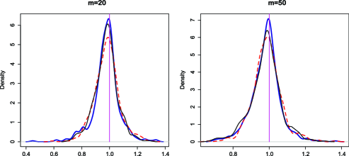
Figure 1: Kernel density plots of the $500$ empirical efficiencies of the two-step estimator to the oracle estimator of the first function $\theta_{1}(\cdot)$ for the IND (dashed lines), EX (thick lines) and AR(1) (thin lines) working correlation structures with $m=20,50$.

We plotted the kernel density estimates in Figure 1 of $500$ empirical efficiencies $\mathrm{eff}_{l,\alpha}$ for the estimators of the first function $\theta_{1}(\cdot)$ for IND (dashed lines), EX (thick lines) and AR(1) (thin lines) structures with $m=20,50$ and $n=250$. The vertical line at $\mbox{efficiency}=1$ is the standard line for the comparison of the two-step estimator (7) and the oracle estimator (5). The centers of density distributions are close to $1$ for all working correlation structures, and EX has the narrowest distribution.

Example 2 ((Binary response)).

The correlated binary responses $\{Y_{ij}\}$ are generated from a marginal logit model

$$\operatorname{logit}P(Y_{ij}=1|\mathbf{X}_{ij},\mathbf{Z}_{ij})=\mathbf{X}_{ij}^{\mathrm{T}}\bolds\beta+\theta_{1}(Z_{ij1})+\theta_{2}(Z_{ij2}),$$

where $\bolds\beta=(0.5,-0.3,0.3)$, $\mathbf{X}_{ij}=(1,X_{ij,1},X_{ij,2})^{\mathrm{T}}$, $\theta_{1}(Z_{1})=0.5\times\sin(2\pi Z_{1})$, and $\theta_{2}(Z_{2})=-0.5\times\{Z_{2}-0.5+\sin(2\pi Z_{2})\}$. For the covariates, we generate $X_{ijk}$ and $Z_{ijl}$ independently from standard normal and uniform distributions, respectively, such that $X_{ijk}\sim\mathrm{N}(0,1)$ and $Z_{ijl}\sim\operatorname{Uniform}[0,1]$. We use the R package “mvtBinaryEP” to generate the correlated binary responses with exchangeable correlation structure with a correlation parameter of $0.1$ within each cluster. We let the number of clusters be $n=100,200,500$, respectively, and let the cluster size be equal and increase with $n$, such that $m_{(n)}=m_{i}=\lfloor 2n^{1/2}\rfloor$, for $1\leq i\leq n$, where $\lfloor a\rfloor$ denotes the largest integer no greater than $a$. So $m=20,28,44$ for $n=100,200,500$, respectively. Table 3 shows the empirical coverage rates of the $95\%$ confidence intervals of the estimators $(\widehat{\beta}_{n,k})_{k=0}^{2}$ for the coefficients $(\beta_{0,k})_{k=0}^{2}$ and the RMSEs for IND, EX and AR(1) and $n=100,200,500$. Table 4 shows that the empirical coverage rates are close to the nominal coverage probabilities $95\%$ for all cases. EX has the smallest RMSE values, and the RMSEs decrease as $n$ increases.

Table 3: The empirical coverage rates of the $95\%$ confidence intervals for $(\beta_{0,k})_{k=0}^{2}$ and the estimated MSE for the IND, EX and AR(1) working correlation structures with $n=100,200,500$

		Coverage frequency			RMSE
		$\bolds{\beta_{0,0}}$	$\bolds{\beta_{0,1}}$	$\bolds{\beta_{0,2}}$	$\bolds{\beta_{0,0}}$	$\bolds{\beta_{0,1}}$	$\bolds{\beta_{0,2}}$
$n=100,m=20$	IND	$0.960$	$0.946$	$0.940$	$0.0821$	$0.0549$	$0.0506$
	EX	$0.940$	$0.946$	$0.946$	$0.0763$	$0.0469$	$0.0454$
	AR(1)	$0.966$	$0.930$	$0.940$	$0.0773$	$0.0540$	$0.0488$
$n=200,m=28$	IND	$0.944$	$0.946$	$0.940$	$0.0559$	$0.0299$	$0.0328$
	EX	$0.948$	$0.952$	$0.942$	$0.0554$	$0.0289$	$0.0310$
	AR(1)	$0.940$	$0.950$	$0.940$	$0.0556$	$0.0291$	$0.0325$
$n=500,m=44$	IND	$0.952$	$0.946$	$0.942$	$0.0340$	$0.0157$	$0.0154$
	EX	$0.948$	$0.952$	$0.946$	$0.0336$	$0.0136$	$0.0142$
	AR(1)	$0.952$	$0.952$	$0.942$	$0.0340$	$0.0153$	$0.0153$

Table 4: The MISE for $\widehat{\theta}_{n,l}^{\mathcal{S}\mathcal{S}}(\cdot)$, $\widehat{\theta}_{n,l}(\cdot)$ and $\widehat{\theta}_{n,l}^{\mathrm{OR}}(\cdot)$, $l=1,2$, for the IND, EX and AR(1) working correlation structures with $n=100,200,500$

$\bolds{n}$		$\bolds{\widehat{\theta}_{n,1}^{\mathcal{S}\mathcal{S}}}$	$\bolds{\widehat{\theta}_{n,1}}$	$\bolds{\widehat{\theta}_{n,1}^{\mathrm{OR}}}$	$\bolds{\widehat{\theta}_{n,2}^{\mathcal{S}\mathcal{S}}}$	$\bolds{\widehat{\theta}_{n,2}}$	$\bolds{\widehat{\theta}_{n,2}^{\mathrm{OR}}}$
$100$	IND	$0.0172$	$0.0243$	$0.0174$	$0.0158$	$0.0222$	$0.0159$
	EX	$0.0148$	$0.0223$	$0.0148$	$0.0139$	$0.0204$	$0.0137$
	AR(1)	$0.0178$	$0.0265$	$0.0176$	$0.0161$	$0.0234$	$0.0163$
$200$	IND	$0.0059$	$0.0086$	$0.0059$	$0.0056$	$0.0082$	$0.0056$
	EX	$0.0048$	$0.0069$	$0.0048$	$0.0054$	$0.0075$	$0.0053$
	AR(1)	$0.0058$	$0.0085$	$0.0058$	$0.0056$	$0.0081$	$0.0056$
$500$	IND	$0.0015$	$0.0022$	$0.0015$	$0.0015$	$0.0021$	$0.0015$
	EX	$0.0013$	$0.0019$	$0.0013$	$0.0014$	$0.0019$	$0.0013$
	AR(1)	$0.0015$	$0.0022$	$0.0015$	$0.0015$	$0.0020$	$0.0014$

Table 4 shows the MISE for the two-step spline estimator $\widehat{\theta}_{n,l}^{\mathcal{S}\mathcal{S}}(\cdot)$, the pilot estimator $\widehat{\theta}_{n,l}(\cdot)$ and the oracle estimator $\widehat{\theta}_{n,l}^{\mathrm{OR}}(\cdot)$, $l=1,2$, for the IND, EX and AR(1) structures and $n=100,200,500$. The MISE values for $\widehat{\theta}_{n,l}^{\mathcal{S}\mathcal{S}}(\cdot)$ and $\widehat{\theta}_{n,l}^{\mathrm{OR}}(\cdot)$ are close and $\widehat{\theta}_{n,l}(\cdot)$ has the largest MISE values. EX has the smallest MISEs among the three working correlation structures, and the MISEs decrease as $n$ increases.

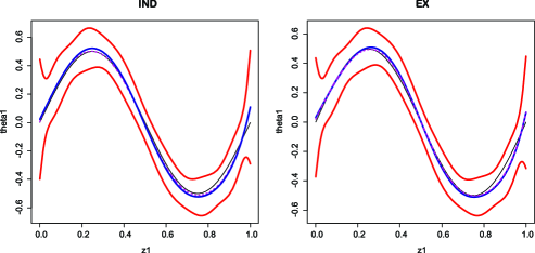
Figure 2: Plots of oracle estimator (dashed curve), the two-step estimator (thick curve) and the $95\%$ pointwise confidence intervals (upper and lower curves) of $\theta_{1}(\cdot)$ (thin curve) for $n=200$.

For visualization of the actual function estimates, in Figure 2 we plotted the oracle estimator given in (5) (dashed curve), the two-step estimator given in (7) (thick curve) and the $95\%$ pointwise confidence intervals constructed in (13) (upper and lower curves) of $\theta_{1}(\cdot)$ (thin curve) for $n=200$ based on one simulated sample. The proposed two-step estimator seems satisfactory.

5 Application

In this section we apply the proposed estimation procedure to analyze unemployment-economic growth and employment relationship at the U.S. state level for the 1970–1986 period. Reference BC05 has first studied the effect of economic growth on unemployment rate by establishing a parametric unemployment-growth model. They concluded that relatively high economic growth is more likely to show reduced unemployment rates when compared to states in which the economy is growing more slowly by obtaining a negative coefficient for growth. Reference W99 demonstrated a strong negative correlation between the change of unemployment rate and employment. We restudy their relationship by considering possible nonlinear relations of the unemployment rate with economic growth and time. The economic growth rate is calculated from the logarithm difference of the gross state product (GSP). The data for the unemployment rate, gross state product and employment are available for the U.S. 48 contiguous states over the period 1970–1986. Details on this data set can be found in M90 . The number of time periods for each state in estimation is $m=16$, since the year 1970 is taken as the initial observation. We consider the following GAPLM:

$$U_{ij}=\beta_{0}+\beta_{1}E_{ij}+\theta_{1}(T_{ij})+\theta_{2}(G_{ij})+\varepsilon_{ij},\qquad j=2,\ldots,17,i=1,\ldots,48,$$

where $U_{ij}$ is the change in the unemployment rate for the $j$th year in the $i$th state, $E_{ij}$ is the empirically centered value of the relative change in employment, $G_{ij}$ is the GSP growth, and $T_{ij}$ is time. $\theta_{1}(\cdot)$ and $\theta_{2}(\cdot)$ are nonparametric functions of time and GSP growth, respectively.

To test whether $\theta_{l}(\cdot)$, $l=1,2$, has a specific parametric form, we construct simultaneous confidence bands according to Theorem 2 of WY09 . For any $\alpha\in(0,1)$, an asymptotic $100(1-\alpha)\%$ conservative confidence band for $\theta_{l0}(z_{l})$ over the domain of $z_{l}$ is given as

$$\widehat{\theta}_{n,l}^{\mathcal{S}}(z_{l},\widehat{\bolds\beta},\widehat{\bolds\theta}_{n,-l})\pm\bigl{\{}2\log\bigl{(}N^{s}+1\bigr{)}-2\log\alpha\bigr{\}}^{1/2}\bigl{(}\mathbf{B}_{l}^{\mathcal{S}}(z_{l})^{\mathrm{T}}\Xi_{n,l}^{\ast}\mathbf{B}_{l}^{\mathcal{S}}(z_{l})\bigr{)}^{1/2}$$

with $\widehat{\theta}_{n,l}^{\mathcal{S}}$ obtained by linear splines with degree $q=1$. We use linear splines in both steps of estimation.

We use three working correlation structures to analyze this data set, including the working independence $\mathbf{R}_{i}(\alpha)=\mathbf{I}_{m}$, where $\mathbf{I}_{m}$ is an $m\times m$ identity matrix, the exchangeable $\mathbf{R}_{i}(\alpha)=\alpha\times 1_{m}1_{m}^{\mathrm{T}}+(1-\alpha)\mathbf{I}_{m}$, where $1_{m}$ is the $m$-dimensional vector with $1$’s, and the AR(1) $\mathbf{R}_{i}(\alpha)=(R_{ijj^{\prime}})_{j,j^{\prime}=1}^{m}$ with $R_{ijj^{\prime}}=\alpha^{|j-j^{\prime}|}$. The parameter $\alpha$ is estimated by the R package geepack from the first spline estimation step. We obtain the estimated values for $\alpha$ which are $\widehat{\alpha}=0.088$ for the EX structure and $\widehat{\alpha}=-0.199$ for the AR(1) structure, respectively. Table 5 shows the estimated

=230pt $\bolds{\widehat{\beta}_{0}}$ $\bolds{\operatorname{SE}(\widehat{\beta}_{0})}$ $\bolds{\widehat{\beta}_{1}}$ $\bolds{\operatorname{SE}(\widehat{\beta}_{1})}$ IND 0.127 0.0417 $-$0.219 0.0230 EX 0.127 0.0494 $-$0.249 0.0220 AR(1) 0.127 0.0484 $-$0.250 0.0216

Table 5: The estimated values $\widehat{\beta}_{0}$ and $\widehat{\beta}_{1}$ of $\beta_{0}$ and $\beta_{1}$ and the standard errors SE$(\widehat{\beta}_{0})$ and SE$(\widehat{\beta}_{1})$ for the IND, EX and AR(1) working correlation structures

values $\widehat{\beta}_{0}$ and $\widehat{\beta}_{1}$ of $\beta_{0}$ and $\beta_{1}$ and the corresponding standard errors SE$(\widehat{\beta}_{0})$ and SE$(\widehat{\beta}_{1})$ for the three working correlation structures. The estimation results are very similar for the three structures. The negative values of $\widehat{\beta}_{1}$ imply a negative relationship between $U_{ij}$ and $E_{ij}$, confirmative to the result in W99 . Both of the estimators are significant with $p$-values close to $0$ for the three different working correlation structures. The correlation coefficient $r=0.785$, $0.822$ and $0.762$ for the IND, EX and AR(1) structures, respectively.

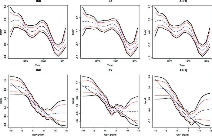
Figure 3: Plots of the two-step spline estimated functions (dashed line), the $95\%$ pointwise confidence intervals (thin lines) and the $95\%$ confidence bands (thick lines) for $\theta_{1}(\cdot)$ (upper panel) and $\theta_{2}(\cdot)$ (lower panel), and the GEE estimator of $\theta_{2}(\cdot)$ by assuming linearity (straight solid line).

Figure 3 displays the two-step spline estimators $\widehat{\theta}_{n,1}^{\mathcal{S}\mathcal{S}}(\cdot)$ (dashed lines) and $\widehat{\theta}_{n,2}^{\mathcal{S}\mathcal{S}}(\cdot)$ (dashed lines) of $\theta_{1}(\cdot)$ and $\theta_{2}(\cdot)$ and the corresponding $95\%$ pointwise confidence intervals (thin lines) and simultaneous confidence bands (thick lines) for the three working structures. Figure 3 shows that the change patterns of $U_{ij}$ with $T_{ij}$ and $G_{ij}$ are very similar for the three working structures. In the upper panel of Figure 3, we can observe a declining trend for $\widehat{\theta}_{n,1}^{\mathcal{S}\mathcal{S}}(\cdot)$ in general. The values of $\widehat{\theta}_{n,1}^{\mathcal{S}\mathcal{S}}(\cdot)$ were all positive before the year $1976$, which means that the unemployment rate was increasing with time during that period. The increasing unemployment rate was caused by a severe economic recession that happened in the years 1973–1975. A local peak of $\widehat{\theta}_{n,1}^{\mathcal{S}\mathcal{S}}(\cdot)$ is observed around $1980$, when another recession happened.

In order to test the linearity of the nonparametric function $\theta_{2}$, we plotted straight solid lines in the lower panel of Figure 3, which are the regression lines obtained by solving the GEE in (2) by assuming that $\theta_{1}(\cdot)$ is a linear function of GSP growth. All the three plots in the lower panel of Figure 3 show that the confidence bands with $95\%$ confidence level do not totally cover the straight regression lines, that is, the linearity of the component function for GSP growth is rejected at the significance level $0.05$. The lower panel of Figure 3 indicates a general negative relation between the GSP growth and the change in unemployment rate.

6 Discussion

In this paper we propose a two-step spline estimating equations procedure for generalized additive partially linear models with large cluster sizes. We develop asymptotic distributions and consistency properties for the two-step estimators of the additive functions and the one-step estimator of the parametric vector. We establish the oracle properties of the two-step estimators. Because the two-step estimator is a mixture of two different spline bases, and an infinite number of observations within clusters are correlated in complex ways, we encountered challenging tasks when developing the theories. We demonstrate our proposed method by two simulated examples and one real data example. Our proposed method can be extended to generalized additive models and generalized additive coefficient models, and it provides a useful tool for studying clustered data. The theoretical development in this paper helps us further investigate semi-parametric models with clustered data. In the real data example, we constructed confidence bands to test the linearity of the nonparametric function. To establish confidence bands with rigorous theoretical proofs will be our future work.

In this paper we focus on the two-step spline estimation procedure, which is computationally expedient and theoretically reliable. As mentioned in Section 2, that kernel smoothing method can be applied to the second step. Let $K_{h}(\cdot)$ be a kernel weight function, where $K_{h}(z)=h^{-1}K(z/h)$ with bandwidth $h$. Let $G_{1}(z_{l})=(1,z_{l})^{\mathrm{T}}$. If we use local linear kernel estimation, then by assuming that $\bolds\beta$ and $\bolds\theta_{-l}$ are known, $\theta_{l}(\cdot)$ is estimated by the oracle estimator $\widehat{\theta}_{l}^{\mathrm{OR}}(Z_{l})=G_{1}(Z_{l}-z_{l})^{\mathrm{T}}\widehat{\bolds\gamma}_{l}^{\mathrm{OR}}$ at any given point $z_{l}$, where $\widehat{\bolds\gamma}_{l}^{\mathrm{OR}}=(\widehat{\gamma}_{l0}^{\mathrm{OR}},\widehat{\gamma}_{l1}^{\mathrm{OR}})^{\mathrm{T}}$ with $\widehat{\bolds\gamma}_{l}^{\mathrm{OR}}$ solving the kernel estimating equations

$$\sum_{i=1}^{n}G_{i1}(z_{l})^{\mathrm{T}}\Delta_{i}\bigl{(}\bolds\beta,\bolds\theta_{-l},\widehat{\bolds\gamma}_{l}^{\mathrm{OR}}\bigr{)}\mathbf{V}_{i}^{-1}\bigl{(}\bolds\beta,\bolds\theta_{-l},\widehat{\bolds\gamma}_{l}^{\mathrm{OR}}\bigr{)}\mathbf{K}_{ih}(z_{l})$$

$$\qquad{}\times\Biggl{\{}\underline{\mathbf{Y}}_{i}-\mu\Biggl{(}\underline{\mathbf{X}}_{i}\bolds\beta+\sum_{l^{\prime}=1,l^{\prime}\neq l}^{d_{2}}\theta_{l^{\prime}}(\mathbf{Z}_{il^{\prime}})+G_{i1}(z_{l})\widehat{\bolds\gamma}_{l}^{\mathrm{OR}}\Biggr{)}\Biggr{\}}=0,$$

where $\mathbf{K}_{ih}(z_{l})=\operatorname{diag}\{K_{h}(Z_{ijl}-z_{l})\}$ and $G_{i1}(z_{l})=\{G_{1}(Z_{i1l}-z_{l}),\ldots,\break G_{1}(Z_{im_{i}l}-z_{l})\}^{\mathrm{T}}$. Then $\theta_{l}(z_{l})$ is estimated by $\widehat{\theta}_{l}^{\mathrm{OR}}(z_{l})=\widehat{\gamma}_{l0}^{\mathrm{OR}}$. The two-step spline backfitted kernel (SBK) estimator $\widehat{\theta}_{l}^{\mathrm{SBK}}(z_{l})$ is obtained by replacing $\bolds\beta$ and $\bolds\theta_{-l}$ with the pilot estimators $\widehat{\bolds\beta}_{n}$ and $\widehat{\bolds\theta}_{n,-l}$ from step I. The asymptotic normality of the oracle estimator $\widehat{\theta}_{l}^{\mathrm{OR}}(z_{l})$ which is a pure local linear kernel estimator of $\theta_{l}(z_{l})$ by GEE can be obtained following the same idea in the proofs for Theorem 3 and the results in LC00 for kernel estimators using GEE. The uniform oracle efficiency of the SBK estimator $\widehat{\theta}_{l}^{\mathrm{SBK}}(z_{l})$ is achievable by following the same procedure as the proofs for Theorem 4 and by studying the properties of spline-kernel combination. See WY07 , LY10 and MY11 for the oracle properties of the SBK estimators in additive models, additive coefficient models and additive partially linear models with weekly-dependent data and a continuous response variable. The asymptotic distributions and the oracle properties of the SBK estimators for GAPLMs with large cluster sizes still need us to explore as future work.

Appendix

We denote by the same letters $c,C$, any positive constants without distinction. For any $s\times s^{\prime}$ matrix $\mathbf{M}$, let $\|\mathbf{M}\|_{\infty}={\max_{1\leq i\leq s}\sum_{j_{=1}}^{s^{\prime}}}|M_{ij}|$. For any vector $\bolds\alpha=(\alpha_{1},\ldots,\alpha_{s})^{\mathrm{T}}$, denote$\|\bolds\alpha\|_{\infty}=\max_{1\leq i\leq s}|\alpha_{i}|$ as the maximum norm. Let $\mathbf{I}_{s}$ be the $s\times s$ identity matrix. Let $\widehat{\Pi}_{n}$, $\Pi_{n}$ denote, respectively, the projection onto $G_{n}^{0}$ relative to the empirical and the theoretical inner products. For any function $\phi$, define the empirical norm as $\|\phi\|_{n_{\mathrm{T}}}^{2}=n_{\mathrm{T}}^{-1}\sum_{i=1}^{n}\sum_{j=1}^{m_{i}}\phi(X_{ij},Z_{ij})^{2}$. For positive numbers $a_{n}$ and $b_{n}$, let $a_{n}\asymp b_{n}$ denote that $\lim_{n\rightarrow\infty}a_{n}/b_{n}=c$, where $c$ is some nonzero constant.

.1 Proof of Theorem 1

It can be proved following the similar reasoning as in MSW12 that under condition (A1) with $n_{\mathrm{T}}\rightarrow\infty$, $J_{n}\rightarrow\infty$, and $J_{n}n^{-1}=o(1)$, there exist constants $0<c^{\prime}<C^{\prime}<\infty$, such that with probability $1$, for $n_{\mathrm{T}}$ sufficiently large,

$$c^{\prime}n_{\mathrm{T}}\leq\lambda_{\mathrm{min}}\Biggl{(}\sum_{i=1}^{n}\underline{\mathbf{B}}_{i}^{\mathrm{T}}\underline{\mathbf{B}}_{i}\Biggr{)}\leq\lambda_{\mathrm{max}}\Biggl{(}\sum_{i=1}^{n}\underline{\mathbf{B}}_{i}^{\mathrm{T}}\underline{\mathbf{B}}_{i}\Biggr{)}\leq C^{\prime}n_{\mathrm{T}}$$

and $\|{\sum_{i=1}^{n}\underline{\mathbf{X}}_{i}^{\mathrm{T}}\underline{\mathbf{B}}_{i}}\|_{\infty}=O_{\mathrm{a.s.}}\{(n_{\mathrm{T}}\log n_{\mathrm{T}})^{1/2}\}$. By these results together with condition (C4), one has with probability $1$,

$$c^{\prime\prime}n_{\mathrm{T}}\leq\lambda_{\mathrm{min}}\Biggl{(}\sum_{i=1}^{n}\underline{\mathbf{D}}_{i}^{\mathrm{T}}\underline{\mathbf{D}}_{i}\Biggr{)}\leq\lambda_{\mathrm{max}}\Biggl{(}\sum_{i=1}^{n}\underline{\mathbf{D}}_{i}^{\mathrm{T}}\underline{\mathbf{D}}_{i}\Biggr{)}\leq C^{\prime\prime}n_{\mathrm{T}}$$ (15)

for some constants $0<c^{\prime\prime}<C^{\prime\prime}<\infty$. Then by condition (A2),

$$\bigl{(}\tau_{n}^{\max}\bigr{)}^{-1}\lambda_{\mathrm{min}}\bigl{\{}\Psi_{n}(\bolds\beta_{0},\bolds\gamma_{0})\bigr{\}}\geq cc^{\prime\prime}\bigl{(}\tau_{n}^{\max}\bigr{)}^{-1}\lambda_{n}^{\min}n_{\mathrm{T}}\rightarrow\infty.$$

Results in Theorem 1 can be proved similarly as Theorems 1 and 2 in XY03 with $r=\sqrt{2(d_{1}+d_{2}J_{n})/c_{0}\varepsilon}$ for any given $\varepsilon>0$.

.2 Proof of Theorem 2

By Taylor’s expansion, one has

$$\mathbf{g}_{n}(\widehat{\bolds\beta}_{n},\widehat{\bolds\gamma}_{n})-\mathbf{g}_{n}(\bolds\beta_{0},\bolds\gamma_{0})=-\mathcal{D}_{n}\bigl{(}\bolds\beta_{n}^{\ast},\bolds\gamma_{n}^{\ast}\bigr{)}\pmatrix{\widehat{\bolds\beta}_{n}-\bolds\beta_{0}\cr\widehat{\bolds\gamma}_{n}-\bolds\gamma_{0}},$$ (16)

where $\bolds\beta_{n}^{\ast}=t_{1}\widehat{\bolds\beta}_{n}+(1-t_{1})\bolds\beta_{0}$, and $\bolds\gamma_{n}^{\ast}=t_{2}\widehat{\bolds\gamma}_{n}+(1-t_{2})\bolds\gamma_{0}$ for some $t_{1},t_{2}\in(0,1)$. Let $\Pi_{i}(\bolds\beta,\bolds\gamma)=\Delta_{i}(\bolds\beta,\bolds\gamma)\mathbf{V}_{i}^{-1}(\bolds\beta,\bolds\gamma)$, for $1\leq i\leq n$. Then

$$\mathcal{D}_{n}\bigl{(}\bolds\beta_{n}^{\ast},\bolds\gamma_{n}^{\ast}\bigr{)}=\Psi_{n}(\bolds\beta_{0},\bolds\gamma_{0})+\Pi_{n,1}\bigl{(}\bolds\beta_{n}^{\ast},\bolds\gamma_{n}^{\ast}\bigr{)}+\Pi_{n,2}\bigl{(}\bolds\beta_{n}^{\ast},\bolds\gamma_{n}^{\ast}\bigr{)}+\Pi_{n,3}+O\bigl{(}n_{\mathrm{T}}J_{n}^{-p}\bigr{)},$$

where $\Pi_{n,1}(\bolds\beta_{n}^{\ast},\bolds\gamma_{n}^{\ast})=-\sum_{i=1}^{n}\underline{\mathbf{D}}_{i}^{\mathrm{T}}\dot{\Pi}_{i}(\bolds\beta_{n}^{\ast},\bolds\gamma_{n}^{\ast})\underline{\bolds\varepsilon}_{i}$,

$$\Pi_{n,2}\bigl{(}\bolds\beta_{n}^{\ast},\bolds\gamma_{n}^{\ast}\bigr{)}=\sum_{i=1}^{n}\underline{\mathbf{D}}_{i}^{\mathrm{T}}\dot{\Pi}_{i}\bigl{(}\bolds\beta_{n}^{\ast},\bolds\gamma_{n}^{\ast}\bigr{)}\Delta_{i}\bigl{(}\bolds\beta_{n}^{\ast\ast},\bolds\gamma_{n}^{\ast\ast}\bigr{)}\underline{\mathbf{D}}_{i}\pmatrix{\bolds\beta_{n}^{\ast}-\bolds\beta_{0}\cr\bolds\gamma_{n}^{\ast}-\bolds\gamma_{0}},$$

$\Pi_{n,3}=\Psi_{n}(\bolds\beta_{0},\bolds\gamma_{0})-\Psi_{n}(\bolds\beta_{n}^{\ast},\bolds\gamma_{n}^{\ast})$, where $\dot{\Pi}_{i}(\bolds\beta_{n}^{\ast},\bolds\gamma_{n}^{\ast})$ is the first order derivative of $\Pi_{i}(\bolds\beta,\bolds\gamma)$ evaluated at $(\bolds\beta_{n}^{\ast\mathrm{T}},\bolds\gamma_{n}^{\ast\mathrm{T}})^{\mathrm{T}}$, which is a $m_{i}\times m_{i}\times(d_{1}+d_{2}J_{n})$-dimensional array, $\bolds\beta_{n}^{\ast\ast}$ is between $\bolds\beta_{n}^{\ast}$ and $\bolds\beta_{0}$, and $\bolds\gamma_{n}^{\ast\ast}$ is between $\bolds\gamma_{n}^{\ast}$ and $\bolds\gamma_{0}$. By conditions (C3) and (C4) and (15), for any given vector $\alpha_{n}\in R^{(d_{1}+d_{2}J_{n})}$ with $\|\alpha_{n}\|=1$, there exists a constant $0<c<\infty$, such that with probability approaching $1$, $\alpha_{n}^{\mathrm{T}}\Psi_{n}(\bolds\beta_{0},\bolds\gamma_{0})\alpha_{n}\geq cn_{\mathrm{T}}\lambda_{n}^{\mathrm{min}}$. By Theorem 1 and (15), $\alpha_{n}^{\mathrm{T}}\Pi_{n,2}(\bolds\beta_{n}^{\ast},\bolds\gamma_{n}^{\ast})\alpha_{n}=o_{p}(\lambda_{n}^{\mathrm{max}})$. Since $E\{\Pi_{n,1}(\bolds\beta_{n}^{\ast},\bolds\gamma_{n}^{\ast})|\cal{X},\cal{Z}\}=0$, it can be proved by Bernstein’s inequality of B98 $\alpha_{n}^{\mathrm{T}}\Pi_{n,1}(\bolds\beta_{n}^{\ast},\bolds\gamma_{n}^{\ast})\alpha_{n}=O_{P}\{(n_{\mathrm{T}}\log n_{\mathrm{T}})^{1/2}\}$. By condition (C1), $\lambda_{n}^{\mathrm{max}}=O(\tau_{n}^{\max})=o(n_{\mathrm{T}}\lambda_{n}^{\min}J_{n}^{-1/2})$. Therefore, $\Psi_{n}(\bolds\beta_{0},\bolds\gamma_{0})$ dominates $\Pi_{n,1}(\bolds\beta_{n}^{\ast},\bolds\gamma_{n}^{\ast})$ and $\Pi_{n,2}(\bolds\beta_{n}^{\ast},\bolds\gamma_{n}^{\ast})$, and by Theorem 1, $\Psi_{n}(\bolds\beta_{0},\bolds\gamma_{0})$ dominates $\Pi_{n,3}(\bolds\beta_{n}^{\ast},\bolds\gamma_{n}^{\ast})$. Thus, from (16), one has

$$\pmatrix{\widehat{\bolds\beta}_{n}-\bolds\beta_{0}\cr\widehat{\bolds\gamma}_{n}-\bolds\gamma_{0}}=\Psi_{n}(\bolds\beta_{0},\bolds\gamma_{0})^{-1}\mathbf{g}_{n}(\bolds\beta_{0},\bolds\gamma_{0})\bigl{\{}1+o_{p}(1)\bigr{\}}.$$ (17)

Let $\Delta_{i0}=\Delta_{i}(\bolds\beta_{0},\bolds\gamma_{0})$ and $\mathbf{V}_{i0}=\mathbf{V}_{i}(\bolds\beta_{0},\bolds\gamma_{0})$. To obtain the closed-form expression of $\widehat{\bolds\beta}_{n}-\bolds\beta_{0}$, we need the following block form of the inverse of $\sum_{i=1}^{n}\underline{\mathbf{D}}_{i}^{\mathrm{T}}\Delta_{i0}\mathbf{V}_{i0}^{-1}\Delta_{i0}\underline{\mathbf{D}}_{i}$:

$$\pmatrix{\displaystyle\sum_{i=1}^{n}\underline{\mathbf{X}}_{i}^{\mathrm{T}}\Delta_{i0}\mathbf{V}_{i0}^{-1}\Delta_{i0}\underline{\mathbf{X}}_{i}&\displaystyle\sum_{i=1}^{n}\underline{\mathbf{X}}_{i}^{\mathrm{T}}\Delta_{i0}\mathbf{V}_{i0}^{-1}\Delta_{i0}\underline{\mathbf{B}}_{i}\vspace*{2pt}\cr\displaystyle\sum_{i=1}^{n}\underline{\mathbf{B}}_{i}^{\mathrm{T}}\Delta_{i0}\mathbf{V}_{i0}^{-1}\Delta_{i0}\underline{\mathbf{X}}_{i}&\displaystyle\sum_{i=1}^{n}\underline{\mathbf{B}}_{i}^{\mathrm{T}}\Delta_{i0}\mathbf{V}_{i0}^{-1}\Delta_{i0}\underline{\mathbf{B}}_{i}}^{-1}$$

(18)

$$\qquad=\pmatrix{\mathbf{H}_{\mathbf{XX}}&\mathbf{H}_{\mathbf{XB}}\cr\mathbf{H}_{\mathbf{BX}}&\mathbf{H}_{\mathbf{BB}}}^{-1}=\pmatrix{\mathbf{H}^{11}&\mathbf{H}^{12}\cr\mathbf{H}^{21}&\mathbf{H}^{22}},$$

where $\mathbf{H}^{11}=(\mathbf{H}_{\mathbf{XX}}-\mathbf{H}_{\mathbf{XB}}\mathbf{H}_{\mathbf{BB}}^{-1}\mathbf{H}_{\mathbf{BX}})^{-1}$, $\mathbf{H}^{22}=(\mathbf{H}_{\mathbf{BB}}-\mathbf{H}_{\mathbf{BX}}\mathbf{H}_{\mathbf{XX}}^{-1}\mathbf{H}_{\mathbf{XB}})^{-1}$, $\mathbf{H}^{12}=-\mathbf{H}^{11}\mathbf{H}_{\mathbf{XB}}\mathbf{H}_{\mathbf{BB}}^{-1}$, and $\mathbf{H}^{21}=-\mathbf{H}^{22}\mathbf{H}_{\mathbf{BX}}\mathbf{H}_{\mathbf{XX}}^{-1}$. Consequently, $\widehat{\bolds\beta}_{n}-\bolds\beta_{0}=(\widetilde{\bolds\beta}_{n,e}+\widetilde{\bolds\beta}_{n,\mu})\{1+o_{p}(1)\}$, in which

$$\widetilde{\bolds\beta}_{n,e} = \mathbf{H}^{11}\Biggl{\{}\sum_{i=1}^{n}\underline{\mathbf{X}}_{i}^{\mathrm{T}}\Delta_{i0}\mathbf{V}_{i0}^{-1}\underline{\bolds\varepsilon}_{i}-\mathbf{H}_{\mathbf{XB}}\mathbf{H}_{\mathbf{BB}}^{-1}\sum_{i=1}^{n}\underline{\mathbf{B}}_{i}^{\mathrm{T}}\Delta_{i0}\mathbf{V}_{i0}^{-1}\underline{\bolds\varepsilon}_{i}\Biggr{\}},$$

$$\widetilde{\bolds\beta}_{n,\mu} = \mathbf{H}^{11}\Biggl{[}\sum_{i=1}^{n}\underline{\mathbf{X}}_{i}^{\mathrm{T}}\Delta_{i0}\mathbf{V}_{i0}^{-1}\Biggl{\{}\mu\Biggl{(}\underline{\mathbf{X}}_{i}\bolds\beta_{0}+\sum_{l=1}^{d_{2}}\theta_{l0}(\mathbf{Z}_{il})\Biggr{)}-\mu(\underline{\mathbf{X}}_{i}\bolds\beta_{0}+\underline{\mathbf{B}}_{i}\bolds\gamma_{0})\Biggr{\}}$$

$$\hskip 21.5pt{}-\mathbf{H}_{\mathbf{XB}}\mathbf{H}_{\mathbf{BB}}^{-1}\sum_{i=1}^{n}\underline{\mathbf{B}}_{i}^{\mathrm{T}}\Delta_{i0}\mathbf{V}_{i0}^{-1}\Biggl{\{}\mu\Biggl{(}\underline{\mathbf{X}}_{i}\bolds\beta_{0}+\sum_{l=1}^{d_{2}}\theta_{l0}(\mathbf{Z}_{il})\Biggr{)}$$

$$\hskip 203.5pt{}-\mu(\underline{\mathbf{X}}_{i}\bolds\beta_{0}+\underline{\mathbf{B}}_{i}\bolds\gamma_{0})\Biggr{\}}\Biggr{]}.$$

Lemma 1

Under condition (A4), there are constants $0<c_{H_{1}}<C_{H_{1}}<\infty$, such that with probability approaching $1$, for $n_{\mathrm{T}}$ sufficiently large,$c_{H_{1}}(\lambda_{n}^{\max}\*n_{\mathrm{T}})^{-1}\mathbf{I}_{d_{1}}\leq\mathbf{H}^{11}\leq C_{H_{1}}(\lambda_{n}^{\max}n_{\mathrm{T}})^{-1}\mathbf{I}_{d_{1}}$ with $\mathbf{H}^{11}$in (.2).

The proof of Lemma 1 follows the same fashion as the proof of Lemma A.4 in MSW12 , and is hence omitted.

Lemma 2

Under conditions (A2) and (A4), $\|\widetilde{\bolds\beta}_{n,\mu}\|=O_{P}\{(\lambda_{n}^{\max}/\lambda_{n}^{\min})\*J_{n}^{-2p}\}$.

Let $\Delta\mu(\underline{\bolds\eta}_{i})=\mu(\underline{\mathbf{X}}_{i}\bolds\beta_{0}+\sum_{l=1}^{d_{2}}\theta_{l0}(\mathbf{Z}_{il}))-\mu(\underline{\mathbf{X}}_{i}\bolds\beta_{0}+\underline{\mathbf{B}}_{i}\bolds\gamma_{0})=\break\{\Delta\mu(\eta_{ij})\}_{j=1}^{m_{i}}$, then

$$\widetilde{\bolds\beta}_{n,\mu} = \mathbf{H}^{11}\Biggl{[}\sum_{i=1}^{n}\underline{\mathbf{X}}_{i}^{\mathrm{T}}\Delta_{i0}\mathbf{V}_{i0}^{-1}\bigl{\{}\Delta\mu(\underline{\bolds\eta}_{i})\bigr{\}}-\mathbf{H}_{\mathbf{XB}}\mathbf{H}_{\mathbf{BB}}^{-1}\sum_{i=1}^{n}\underline{\mathbf{B}}_{i}^{\mathrm{T}}\Delta_{i0}\mathbf{V}_{i0}^{-1}\bigl{\{}\Delta\mu(\underline{\bolds\eta}_{i})\bigr{\}}\Biggr{]}$$

$$= \mathbf{H}^{11}\sum_{i=1}^{n}\underline{\mathbf{X}}_{i}^{\mathrm{T}}\Delta_{i0}\mathbf{V}_{i0}^{-1}\bigl{[}\bigl{\{}\Delta\mu(\underline{\bolds\eta}_{i})\bigr{\}}-\widehat{\Pi}_{n}\bigl{\{}\Delta\mu(\underline{\bolds\eta}_{i})\bigr{\}}\bigr{]}=n_{\mathrm{T}}\mathbf{H}^{11}\mathbf{W},$$

where $\mathbf{W}=(W_{1},\ldots,W_{d_{1}})$, with

$$|W_{k}| = n_{\mathrm{T}}^{-1}\Biggl{|}\sum_{i=1}^{n}\bigl{(}\underline{\mathbf{X}}_{i}^{(k)}\bigr{)}^{\mathrm{T}}\Delta_{i0}\mathbf{V}_{i0}^{-1}\bigl{[}\bigl{\{}\Delta\mu(\underline{\bolds\eta}_{i})\bigr{\}}-\widehat{\Pi}_{n}\bigl{\{}\Delta\mu(\underline{\bolds\eta}_{i})\bigr{\}}\bigr{]}\Biggr{|}$$

$$\leq C\lambda_{n}^{\max}n_{\mathrm{T}}^{-1}\sum_{i=1}^{n}\sum_{j=1}^{m_{i}}\bigl{|}X_{ijk}\bigl{\{}\Delta\mu(\eta_{ij})\bigr{\}}-\widehat{\Pi}_{n}\bigl{\{}\Delta\mu(\eta_{ij})\bigr{\}}\bigr{|}.$$

Following similar reasoning as in the proof of Lemma A.5 in MSW12 , it can be proved that $n_{\mathrm{T}}^{-1}\sum_{i=1}^{n}\sum_{j=1}^{m_{i}}|X_{ijk}\{\Delta\mu(\eta_{ij})\}-\widehat{\Pi}_{n}\{\Delta\mu(\eta_{ij})\}|=O_{P}(J_{n}^{-2p})$. Therefore, $|W_{k}|=O_{P}(\lambda_{n}^{\max}J_{n}^{-2p})$. By the above result and Lemma 1, one has $\|\widetilde{\bolds\beta}_{n,\mu}\|=O_{P}\{(\lambda_{n}^{\min})^{-1}\lambda_{n}^{\max}J_{n}^{-2p}\}$.

Lemma 3

Under conditions (A2)–(A4), as $n_{\mathrm{T}}\rightarrow\infty$, $\widetilde{\Xi}_{n}^{-1/2}(\widetilde{\bolds\beta}_{n,e})\longrightarrow N(0,\mathbf{I}_{d_{1}})$, where $\widetilde{\Xi}_{n}$ is defined in (9).

Lemma 3 can be proved by using the Linderberg–Feller CLT and similar techniques for the proofs of Lemmas A.6 and A.7 in MSW12 .

Lemma 4

Under conditions (A2) and (A4), there exist constants $0<c_{\Xi}\leq C_{\Xi}<\infty$, such that

$$c_{\Xi}n_{\mathrm{T}}^{-1}\bigl{(}\lambda_{n}^{\max}\bigr{)}^{-1}\tau_{n}^{\min}\mathbf{I}_{d_{1}}\leq\widetilde{\Xi}_{n}\leq C_{\Xi}n_{\mathrm{T}}^{-1}\tau_{n}^{\max}\bigl{(}\lambda_{n}^{\min}\bigr{)}^{-1}\mathbf{I}_{d_{1}}$$

and $\|\widetilde{\bolds\beta}_{n,e}\|=O_{p}\{n_{\mathrm{T}}^{-1/2}(\tau_{n}^{\max})^{1/2}(\lambda_{n}^{\min})^{-1/2}\}$.

For any vector $a\in R^{d_{1}}$ with $\|a\|=1$, one has

$$a^{\mathrm{T}}\widetilde{\Xi}_{n}a \leq \tau_{n}^{\max}a^{\mathrm{T}}\Biggl{\{}E\Biggl{(}\sum_{i=1}^{n}\widetilde{\underline{\mathbf{X}}}_{i}^{\mathrm{T}}\Delta_{i0}\mathbf{V}_{i0}^{-1}\Delta_{i0}\widetilde{\underline{\mathbf{X}}}_{i}\Biggr{)}\Biggr{\}}^{-1}a\leq C_{\Xi}n_{\mathrm{T}}^{-1}\tau_{n}^{\max}\bigl{(}\lambda_{n}^{\min}\bigr{)}^{-1},$$

$$a^{\mathrm{T}}\widetilde{\Xi}_{n}a \geq \Biggl{\{}E\Biggl{(}\sum_{i=1}^{n}\widetilde{\underline{\mathbf{X}}}_{i}^{\mathrm{T}}\Delta_{i0}\mathbf{V}_{i0}^{-1}\Delta_{i0}\widetilde{\underline{\mathbf{X}}}_{i}\Biggr{)}\Biggr{\}}^{-1}\tau_{n}^{\min}\geq c_{\Xi}n_{\mathrm{T}}^{-1}\bigl{(}\lambda_{n}^{\max}\bigr{)}^{-1}\tau_{n}^{\min},$$

and the second result in Lemma 4 follows from Chebyshev’s inequality. Proof of Theorem 2 By Lemmas 2 and 4, for any vector $a\in R^{d_{1}}$ with $\|a\|=1$, one has

$$a^{\mathrm{T}}\widetilde{\Xi}_{n}^{-1/2}\widetilde{\bolds\beta}_{n,\mu}a \leq c_{\Xi}^{-1/2}n_{\mathrm{T}}^{1/2}\bigl{(}\lambda_{n}^{\max}\bigr{)}^{1/2}\bigl{(}\tau_{n}^{\min}\bigr{)}^{-1/2}O_{P}\bigl{\{}\bigl{(}\lambda_{n}^{\min}\bigr{)}^{-1}\lambda_{n}^{\max}J_{n}^{-2p}\bigr{\}}$$

$$= O_{P}\bigl{\{}n_{\mathrm{T}}^{1/2}J_{n}^{-2p}\bigl{(}\lambda_{n}^{\max}\bigr{)}^{3/2}\bigl{(}\lambda_{n}^{\min}\bigr{)}^{-1}\bigl{(}\tau_{n}^{\min}\bigr{)}^{-1/2}\bigr{\}}=o_{p}(1).$$

Therefore, Theorem 2 follows from Lemma 3, the above result and Slutsky’s theorem.

.3 Proof of Theorem 3

Following the same reasoning as deriving (17), it can be proved that

$$\widehat{\bolds\gamma}_{n,l}^{\mathcal{S}}(\bolds\beta_{0},\bolds\theta_{-l0})-\bolds\gamma_{l,0}^{\mathcal{S}} = \Psi_{n,l}^{\ast}\bigl{(}\bolds\gamma_{l,0}^{\mathcal{S}}\bigr{)}^{-1}\mathbf{g}_{n,l}^{\ast}(\bolds\gamma_{l,0})\bigl{(}1+o_{p}(1)\bigr{)}$$

$$= \bigl{(}\widetilde{\bolds\gamma}_{n,e,l}^{\mathcal{S}}+\widetilde{\bolds\gamma}_{n,\mu,l}^{\mathcal{S}}\bigr{)}\bigl{(}1+o_{p}(1)\bigr{)},$$

where

$$\widetilde{\bolds\gamma}_{n,e,l}^{\mathcal{S}} = \widetilde{\bolds\gamma}_{n,e,l}^{\mathcal{S}}(\bolds\beta_{0},\bolds\theta_{-l0})$$

$$= \Psi_{n,l}^{\ast}\bigl{(}\bolds\gamma_{l,0}^{\mathcal{S}}\bigr{)}^{-1}\sum_{i=1}^{n}\bigl{(}\mathbf{B}_{i\cdot l}^{\mathcal{S}}\bigr{)}^{\mathrm{T}}\Delta_{i}\bigl{(}\bolds\beta_{0},\bolds\theta_{-l0},\bolds\gamma_{l,0}^{\mathcal{S}}\bigr{)}\mathbf{V}_{i}^{-1}\bigl{(}\bolds\beta_{0},\bolds\theta_{-l0},\bolds\gamma_{l,0}^{\mathcal{S}}\bigr{)}\underline{\bolds\varepsilon}_{i},$$

$$\widetilde{\bolds\gamma}_{n,\mu,l}^{\mathcal{S}} = \widetilde{\bolds\gamma}_{n,\mu,l}^{\mathcal{S}}(\bolds\beta_{0},\bolds\theta_{-l0})=\bigl{(}\widetilde{\gamma}_{n,\mu,sl}^{\mathcal{S}}\bigr{)}_{s=1}^{J_{n}^{\mathcal{S}}}$$

$$= \Psi_{n,l}^{\ast}\bigl{(}\bolds\gamma_{l,0}^{\mathcal{S}}\bigr{)}^{-1}\sum_{i=1}^{n}\bigl{(}\mathbf{B}_{i\cdot l}^{\mathcal{S}}\bigr{)}^{\mathrm{T}}\Delta_{i}\bigl{(}\bolds\beta_{0},\bolds\theta_{-l0},\bolds\gamma_{l,0}^{\mathcal{S}}\bigr{)}\mathbf{V}_{i}^{-1}\bigl{(}\bolds\beta_{0},\bolds\theta_{-l0},\bolds\gamma_{l,0}^{\mathcal{S}}\bigr{)}$$

$$\hskip 70.2pt{}\times\biggl{\{}\mu\biggl{(}\underline{\mathbf{X}}_{i}\bolds\beta_{0}+\sum_{l^{\prime}\neq l}\theta_{l^{\prime}0}(\mathbf{Z}_{il^{\prime}})+\theta_{l0}(\mathbf{Z}_{il})\biggr{)}$$

$$\hskip 87.4pt{}-\mu\biggl{(}\underline{\mathbf{X}}_{i}\bolds\beta_{0}+\sum_{l^{\prime}\neq l}\theta_{l^{\prime}0}(\mathbf{Z}_{il^{\prime}})+\mathbf{B}_{i\cdot l}^{\mathcal{S}}\bolds\gamma_{l,0}^{\mathcal{S}}\biggr{)}\biggr{\}}.$$

By the decomposition in (.3),

$$\widehat{\theta}_{n,l}^{\mathcal{S}}(z_{l},\bolds\beta_{0},\bolds\theta_{-l0})-\theta_{l0}^{\ast}(z_{l}) = \mathbf{B}_{l}^{\mathcal{S}}(z_{l})^{\mathrm{T}}\widetilde{\bolds\gamma}_{n,e,l}^{\mathcal{S}}\bigl{(}1+o_{p}(1)\bigr{)},$$

$$\theta_{l0}^{\ast}(z_{l})-\theta_{l0}(z_{l}) = \bigl{\{}\mathbf{B}_{l}^{\mathcal{S}}(z_{l})^{\mathrm{T}}\widetilde{\bolds\gamma}_{n,\mu,l}^{\mathcal{S}}+\mathbf{B}_{l}^{\mathcal{S}}(z_{l})^{\mathrm{T}}\bolds\gamma_{l,0}^{\mathcal{S}}-\theta_{l0}(z_{l})\bigr{\}}$$

$${}\times\bigl{(}1+o_{p}(1)\bigr{)}.$$

It can be proved by the Linderberg–Feller CLT that as $n_{\mathrm{T}}\rightarrow\infty$,

$$\bigl{(}\mathbf{B}_{l}^{\mathcal{S}}(z_{l})^{\mathrm{T}}\Xi_{n,l}^{\ast}\mathbf{B}_{l}^{\mathcal{S}}(z_{l})\bigr{)}^{-1/2}\bigl{(}\mathbf{B}_{l}^{\mathcal{S}}(z_{l})^{\mathrm{T}}\widetilde{\bolds\gamma}_{n,e,l}^{\mathcal{S}}\bigr{)}\longrightarrow N(0,1).$$

Following similar reasoning as in the proofs in Lemma 5, it can be proved

$$\sup_{1\leq s\leq J_{n}^{\mathcal{S}}}\bigl{|}\widetilde{\gamma}_{n,\mu,sl}^{\mathcal{S}}\bigr{|}=O_{P}\bigl{\{}\bigl{(}\lambda_{n}^{\min}\bigr{)}^{-1}\lambda_{n}^{\max}\bigl{(}J_{n}^{\mathcal{S}}\bigr{)}^{-p-1/2}\bigr{\}}$$

and

$$\bigl{\|}\widetilde{\bolds\gamma}_{n,\varepsilon,l}^{\mathcal{S}}\bigr{\|}_{\infty}=O_{P}\bigl{\{}(\log n_{\mathrm{T}}/n_{\mathrm{T}})^{1/2}\bigl{(}\tau_{n}^{\max}\bigr{)}^{1/2}\bigl{(}\lambda_{n}^{\min}\bigr{)}^{-1/2}\bigr{\}}.$$

By B-spline properties, $\sup_{z_{l}\in[0,1]}|\mathbf{B}_{l}^{\mathcal{S}}(z_{l})^{\mathrm{T}}\widetilde{\bolds\gamma}_{n,\mu,l}^{\mathcal{S}}|=O_{P}\{(\lambda_{n}^{\max}/\lambda_{n}^{\min})(J_{n}^{\mathcal{S}})^{-p}\}$, and $\sup_{z_{l}\in[0,1]}|\mathbf{B}_{l}^{\mathcal{S}}(z_{l})^{\mathrm{T}}\widetilde{\bolds\gamma}_{n,\varepsilon,l}^{\mathcal{S}}|=O_{P}\{\sqrt{(\log n_{\mathrm{T}})J_{n}^{\mathcal{S}}/n_{\mathrm{T}}}(\tau_{n}^{\max}/\lambda_{n}^{\min})^{1/2}\}$, so

$$\sup_{z_{l}\in[0,1]}\bigl{|}\theta_{l0}^{\ast}(z_{l})-\theta_{l0}(z_{l})\bigr{|} \leq \sup_{z_{l}\in[0,1]}\bigl{|}\mathbf{B}_{l}^{\mathcal{S}}(z_{l})^{\mathrm{T}}\widetilde{\bolds\gamma}_{n,\mu,l}^{\mathcal{S}}\bigr{|}$$

$${}+\sup_{z_{l}\in[0,1]}\bigl{|}\mathbf{B}_{l}^{\mathcal{S}}(z_{l})^{\mathrm{T}}\bolds\gamma_{l,0}^{\mathcal{S}}-\theta_{l0}(z_{l})\bigr{|}$$

$$= O_{P}\bigl{\{}\bigl{(}\lambda_{n}^{\min}\bigr{)}^{-1}\lambda_{n}^{\max}\bigl{(}J_{n}^{\mathcal{S}}\bigr{)}^{-p}\bigr{\}},$$

$\sup_{z_{l}\in[0,1]}|\widehat{\theta}_{n,l}^{\mathcal{S}}(z_{l},\bolds\beta_{0},\bolds\theta_{-l0})-\theta_{l0}^{\ast}(z_{l})|=O_{P}\{\sqrt{(\log n_{\mathrm{T}})J_{n}^{\mathcal{S}}/n_{\mathrm{T}}}(\tau_{n}^{\max}/\lambda_{n}^{\min})^{1/2}\}$.

.4 Proof of Theorem 4

Lemma 5

Under conditions (A2)–(A4),

$$\|\widehat{\bolds\gamma}_{n}-\bolds\gamma_{0}\| = O_{P}\bigl{\{}J_{n}^{1/2}n_{\mathrm{T}}^{-1/2}\bigl{(}\tau_{n}^{\max}/\lambda_{n}^{\min}\bigr{)}^{1/2}+\bigl{(}\lambda_{n}^{\max}/\lambda_{n}^{\min}\bigr{)}J_{n}^{-p}\bigr{\}},$$

$$\|\widehat{\bolds\gamma}_{n}-\bolds\gamma_{0}\|_{\infty} = O_{P}\bigl{\{}(\log n_{\mathrm{T}}/n_{\mathrm{T}})^{1/2}\bigl{(}\tau_{n}^{\max}/\lambda_{n}^{\min}\bigr{)}^{1/2}+\bigl{(}\lambda_{n}^{\max}/\lambda_{n}^{\min}\bigr{)}J_{n}^{-p-1/2}\bigr{\}}.$$

From (17) and (.2), one obtains $\widehat{\bolds\gamma}_{n}-\bolds\gamma_{0}=(\widetilde{\bolds\gamma}_{n,e}+\widetilde{\bolds\gamma}_{n,\mu})(1+o_{p}(1))$, where

$$\widetilde{\bolds\gamma}_{n,e} = \mathbf{H}^{22}\Biggl{\{}\sum_{i=1}^{n}\underline{\mathbf{B}}_{i}^{\mathrm{T}}\Delta_{i0}\mathbf{V}_{i0}^{-1}\underline{\bolds\varepsilon}_{i}-\mathbf{H}_{\mathbf{BX}}\mathbf{H}_{\mathbf{XX}}^{-1}\sum_{i=1}^{n}\underline{\mathbf{X}}_{i}^{\mathrm{T}}\Delta_{i0}\mathbf{V}_{i0}^{-1}\underline{\bolds\varepsilon}_{i}\Biggr{\}},$$

$$\widetilde{\bolds\gamma}_{n,\mu} = \mathbf{H}^{22}\Biggl{[}\sum_{i=1}^{n}\underline{\mathbf{B}}_{i}^{\mathrm{T}}\Delta_{i0}\mathbf{V}_{i0}^{-1}\Biggl{\{}\mu\Biggl{(}\underline{\mathbf{X}}_{i}\bolds\beta_{0}+\sum_{l=1}^{d_{2}}\theta_{l0}(\mathbf{Z}_{il})\Biggr{)}-\mu(\underline{\mathbf{X}}_{i}\bolds\beta_{0}+\underline{\mathbf{B}}_{i}\bolds\gamma_{0})\Biggr{\}}$$

$$\hskip 22.0pt{}-\mathbf{H}_{\mathbf{BX}}\mathbf{H}_{\mathbf{XX}}^{-1}\sum_{i=1}^{n}\underline{\mathbf{X}}_{i}^{\mathrm{T}}\Delta_{i0}\mathbf{V}_{i0}^{-1}\Biggl{\{}\mu\Biggl{(}\underline{\mathbf{X}}_{i}\bolds\beta_{0}+\sum_{l=1}^{d_{2}}\theta_{l0}(\mathbf{Z}_{il})\Biggr{)}$$

$$\hskip 203.0pt{}-\mu(\underline{\mathbf{X}}_{i}\bolds\beta_{0}+\underline{\mathbf{B}}_{i}\bolds\gamma_{0})\Biggr{\}}\Biggr{]}.$$

It can be proved that there exist constants $0<c_{H_{2}}<C_{H_{2}}<\infty$, such that with probability approaching $1$, for $n_{\mathrm{T}}$ sufficiently large,

$$c_{H_{2}}\bigl{(}\lambda_{n}^{\max}\bigr{)}^{-1}n_{\mathrm{T}}^{-1}\mathbf{I}_{d_{1}}\leq\mathbf{H}^{22}\leq C_{H_{2}}\bigl{(}\lambda_{n}^{\min}\bigr{)}^{-1}n_{\mathrm{T}}^{-1}\mathbf{I}_{d_{1}}.$$

Letting $\widehat{\Pi}_{n,\mathbf{X}}$ be the projection on $\{\underline{\mathbf{X}}_{i}\}_{i=1}^{n}$ to the empirical inner product,

$$\widetilde{\bolds\gamma}_{n,\mu}=\mathbf{H}^{22}\sum_{i=1}^{n}\underline{\mathbf{B}}_{i}^{\mathrm{T}}\Delta_{i0}\mathbf{V}_{i0}^{-1}\bigl{[}\bigl{\{}\Delta\mu(\underline{\bolds\eta}_{i})\bigr{\}}-\widehat{\Pi}_{n,\mathbf{X}}\bigl{\{}\Delta\mu(\underline{\bolds\eta}_{i})\bigr{\}}\bigr{]}=n_{\mathrm{T}}\mathbf{H}^{22}\mathbf{W},$$

where $\mathbf{W}=(W_{1},\ldots,W_{J_{n}d_{2}})$, with

$$W_{s,l}=n_{\mathrm{T}}^{-1}\sum_{i=1}^{n}\bigl{(}\mathbf{B}_{i}^{(s,l)}\bigr{)}^{\mathrm{T}}\Delta_{i0}\mathbf{V}_{i0}^{-1}\bigl{[}\bigl{\{}\Delta\mu(\underline{\bolds\eta}_{i})\bigr{\}}-\widehat{\Pi}_{n,\mathbf{X}}\bigl{\{}\Delta\mu(\underline{\bolds\eta}_{i})\bigr{\}}\bigr{]},$$

$\mathbf{B}_{i}^{(s,l)}=[\{B_{s,l}(Z_{i1l}),\ldots,B_{s,l}(Z_{im_{i}l})\}^{\mathrm{T}}]$. The Cauchy–Schwarz inequality implies

$$|W_{s,l}| \leq C\lambda_{n}^{\max}n_{\mathrm{T}}^{-1}\sum_{i=1}^{n}\sum_{j=1}^{m_{i}}\bigl{|}B_{s,l}(Z_{ijl})\bigl{\{}\Delta\mu(\eta_{ij})\bigr{\}}-\widehat{\Pi}_{n,\mathbf{X}}\bigl{\{}\Delta\mu(\eta_{ij})\bigr{\}}\bigr{|}$$

$$\leq C\lambda_{n}^{\max}\|B_{s,l}\|_{n_{\mathrm{T}}}\bigl{\|}\Delta\mu-\widehat{\Pi}_{n,\mathbf{X}}(\Delta\mu)\bigr{\|}_{n_{\mathrm{T}}}=O_{P}\bigl{(}\lambda_{n}^{\max}J_{n}^{-p-1/2}\bigr{)},$$

thus, $\|\widetilde{\bolds\gamma}_{n,\mu}\|=O_{P}\{(\lambda_{n}^{\max}/\lambda_{n}^{\min})J_{n}^{-p}\}$, $\|\widetilde{\bolds\gamma}_{n,\mu}\|_{\infty}=O_{P}\{(\lambda_{n}^{\max}/\lambda_{n}^{\min})J_{n}^{-p-1/2}\}$. For any $\omega\in\cal{R}^{J_{n}d_{2}}$ with $\|\omega\|=1$, it can be proved that $\operatorname{Var}(\omega^{\mathrm{T}}\widetilde{\bolds\gamma}_{n,e}|\cal{X},\cal{Z})\leq O_{P}\{n_{\mathrm{T}}^{-1}(\tau_{n}^{\max}/\lambda_{n}^{\min})\}$, thus, $\omega^{\mathrm{T}}\widetilde{\bolds\gamma}_{n,e}=O_{P}\{n_{\mathrm{T}}^{-1/2}(\tau_{n}^{\max}/\lambda_{n}^{\min})^{1/2}\}$. Therefore, $\|\widetilde{\bolds\gamma}_{n,e}\|\leq J_{n}^{1/2}|\omega^{\mathrm{T}}\widetilde{\bolds\gamma}_{n,e}|=O_{P}\{J_{n}^{1/2}n_{\mathrm{T}}^{-1/2}(\tau_{n}^{\max}/\lambda_{n}^{\min})^{1/2}\}$, and by Bernstein’s inequality of B98 that $\|\widetilde{\bolds\gamma}_{n,e}\|_{\infty}=O_{P}\{(\log n_{\mathrm{T}}/n_{\mathrm{T}})^{1/2}(\tau_{n}^{\max}/\lambda_{n}^{\min})^{1/2}\}$.

Lemma 6

Under conditions (A2)–(A4),

$$\bigl{\|}\widehat{\bolds\gamma}_{n,l}^{\mathcal{S}\mathcal{S}}-\widehat{\bolds\gamma}_{n,l}^{\mathrm{OR}}\bigr{\|}_{\infty}=O_{p}\Bigl{\{}\bigl{(}\lambda_{n}^{\max}/\lambda_{n}^{\min}\bigr{)}^{2}\Bigl{(}\sqrt{\log n_{\mathrm{T}}/\bigl{(}J_{n}^{\mathcal{S}}n_{\mathrm{T}}\bigr{)}}+\bigl{(}J_{n}^{\mathcal{S}}\bigr{)}^{-1/2}J_{n}^{-p}\Bigr{)}\Bigr{\}}.$$

Let $\widetilde{\bolds\theta}_{-l0}=\{\widetilde{\theta}_{l^{\prime}0}(\cdot),l^{\prime}\neq l\}$, where $\widetilde{\theta}_{l^{\prime}0}(\cdot)$ is defined in (8). Let $\widehat{\bolds\gamma}_{n,-l}=(\widehat{\gamma}_{n,sl^{\prime}}\dvtx 1\leq s\leq J_{n},l^{\prime}\neq l)^{\mathrm{T}}$ and $\bolds\gamma_{-l0}=(\gamma_{sl^{\prime},0}\dvtx 1\leq s\leq J_{n},l^{\prime}\neq l)^{\mathrm{T}}$. By the Taylor expansion, $\mathbf{g}_{n,l}^{\mathcal{S}}(\widehat{\bolds\gamma}_{n,l}^{\mathrm{OR}},\widehat{\bolds\beta}_{n},\widehat{\bolds\theta}_{n,-l})-\mathbf{g}_{n,l}^{\mathcal{S}}(\widehat{\bolds\gamma}_{n,l}^{\mathrm{OR}},\widehat{\bolds\beta}_{n},\widetilde{\bolds\theta}_{-l0})=\{\partial\mathbf{g}_{n,l}^{\mathcal{S}}(\widehat{\bolds\gamma}_{n,l}^{\mathrm{OR}},\break\widehat{\bolds\beta}_{n},\widetilde{\bolds\theta}_{-l})/\partial\widetilde{\bolds\gamma}_{-l}^{\mathrm{T}}\}(\widehat{\bolds\gamma}_{n,-l}-\bolds\gamma_{-l0})$, where $\widetilde{\bolds\gamma}_{-l}=t\bolds\gamma_{-l0}+(1-t)\widehat{\bolds\gamma}_{n,-l}$ for $t\in(0,1)$. Let $\widehat{\Delta}_{i}=\Delta_{i}(\widehat{\bolds\beta}_{n},\widetilde{\bolds\theta}_{-l},\widehat{\bolds\gamma}_{n,l}^{\mathrm{OR}})$, $\widehat{\mathbf{V}}_{i}=\mathbf{V}_{i}(\widehat{\bolds\beta}_{n},\widetilde{\bolds\theta}_{-l},\widehat{\bolds\gamma}_{n,l}^{\mathrm{OR}})$, $\widetilde{\underline{\bolds\varepsilon}_{i}}=\underline{\bolds\varepsilon}_{i}-\widehat{\Pi}_{n,\mathbf{X}}(\underline{\bolds\varepsilon}_{i})$,$\widetilde{\Delta\mu}(\underline{\bolds\eta}_{i})=\Delta\mu(\underline{\bolds\eta}_{i})-\widehat{\Pi}_{n,\mathbf{X}}\{\Delta\mu(\underline{\bolds\eta}_{i})\}$, $\mathbf{B}_{ij,-l}=\{(\mathbf{B}_{ijl^{\prime}}^{\mathrm{T}},l^{\prime}\neq l)^{\mathrm{T}}\}_{(d_{2}-1)J_{n}\times 1}$,$\mathbf{B}_{i,-l}=\{(\mathbf{B}_{i1,-l},\ldots,\mathbf{B}_{im_{i},-l})^{\mathrm{T}}\}_{m_{i}\times(d_{2}-1)J_{n}}$. Thus, by (2) and the proofs for Lemma 5, with probability approaching $1$, there are constants $0<C_{1,}C_{2}<\infty$ such that

$$\bigl{\|}\mathbf{g}_{n,l}^{\mathcal{S}}\bigl{(}\widehat{\bolds\gamma}_{n,l}^{\mathrm{OR}},\widehat{\bolds\beta}_{n},\widehat{\bolds\theta}_{n,-l}\bigr{)}-\mathbf{g}_{n,l}^{\mathcal{S}}\bigl{(}\widehat{\bolds\gamma}_{n,l}^{\mathrm{OR}},\widehat{\bolds\beta}_{n},\widetilde{\bolds\theta}_{-l0}\bigr{)}\bigr{\|}_{\infty}$$

$$\qquad\leq C_{1}\bigl{(}\lambda_{n}^{\min}\bigr{)}^{-1}n_{\mathrm{T}}^{-1}$$

$$\qquad\quad{}\times\Biggl{\|}\Biggl{(}\sum_{i=1}^{n}\bigl{(}\mathbf{B}_{i\cdot l}^{\mathcal{S}}\bigr{)}^{\mathrm{T}}\widehat{\Delta}_{i}\widehat{\mathbf{V}}_{i}^{-1}\mathbf{B}_{i,-l}\Biggr{)}\Biggl{\{}\sum_{i=1}^{n}\mathbf{B}_{i,-l}^{\mathrm{T}}\Delta_{i0}\mathbf{V}_{i0}^{-1}\bigl{(}\widetilde{\underline{\bolds\varepsilon}}_{i}+\widetilde{\Delta\mu}(\underline{\bolds\eta}_{i})\bigr{)}\Biggr{\}}\Biggr{\|}_{\infty}$$

$$\qquad\leq C_{2}\bigl{(}\lambda_{n}^{\min}\bigr{)}^{-1}\bigl{(}\|\zeta_{1}\|_{\infty}+\|\zeta_{2}\|_{\infty}\bigr{)},$$

where $\zeta_{1}=n_{\mathrm{T}}^{-1}\{\sum_{i=1}^{n}(\mathbf{B}_{i\cdot l}^{\mathcal{S}})^{\mathrm{T}}\Delta_{i0}\mathbf{V}_{i0}^{-1}\mathbf{B}_{i,-l}\}\{\sum_{i=1}^{n}\mathbf{B}_{i,-l}^{\mathrm{T}}\Delta_{i0}\mathbf{V}_{i0}^{-1}(\widetilde{\Delta\mu}(\underline{\bolds\eta}_{i}))\}$,$\zeta_{2}=n_{\mathrm{T}}^{-1}\{\sum_{i=1}^{n}(\mathbf{B}_{i\cdot l}^{\mathcal{S}})^{\mathrm{T}}\Delta_{i0}\mathbf{V}_{i0}^{-1}\mathbf{B}_{i,-l}\}(\sum_{i=1}^{n}\mathbf{B}_{i,-l}^{\mathrm{T}}\Delta_{i0}\mathbf{V}_{i0}^{-1}\widetilde{\underline{\bolds\varepsilon}}_{i})$, and then$\|\zeta_{1}\|_{\infty}\leq(\lambda_{n}^{\max})^{2}\|\zeta_{3}\|_{\infty}O(J_{n}^{-p})$, where $\zeta_{3}=\Delta_{1}+\Delta_{2}+\Delta_{3}$, $\Delta_{1}=(\delta_{1s})_{s=1}^{J_{n}^{\mathcal{S}}}$, $\Delta_{2}=(\delta_{2s})_{s=1}^{J_{n}^{\mathcal{S}}}$ and $\Delta_{3}=(\delta_{3s})_{s=1}^{J_{n}^{\mathcal{S}}}$ with $\delta_{1s}=n_{\mathrm{T}}^{-1}\sum_{i=1}^{n}\delta_{1s,i}$, $\delta_{2s}=n_{\mathrm{T}}^{-1}\sum_{i=1}^{n}\delta_{2s,i}$ and $\delta_{3s}=n_{\mathrm{T}}^{-1}\sum_{i=1}^{n}\delta_{3s,i}$,

$$\delta_{1s,i} = \sum_{j=1}^{m_{i}}\sum_{l^{\prime}=1,l^{\prime}\neq l}^{d_{2}}\sum_{s^{\prime}=1}^{J_{n}}\bigl{|}B_{s,l}^{\mathcal{S}}(Z_{ijl})\bigr{|}\bigl{|}B_{s^{\prime},l^{\prime}}(Z_{ijl^{\prime}})\bigr{|}^{2},$$

$$\delta_{2s,i} = \sum_{j=1}^{m_{i}}\sum_{j\prime\neq j}\sum_{l^{\prime}\neq l}\sum_{s^{\prime}=1}^{J_{n}}\bigl{|}B_{s,l}^{\mathcal{S}}(Z_{ijl})\bigr{|}\bigl{|}B_{s^{\prime},l^{\prime}}(Z_{ijl^{\prime}})\bigr{|}\bigl{|}B_{s^{\prime},l^{\prime}}(Z_{ij^{\prime}l^{\prime}})\bigr{|},$$

$$\delta_{3s,i} = \sum_{j=1}^{m_{i}}\sum_{i^{\prime}\neq i}\sum_{j^{\prime}}\sum_{l^{\prime}\neq l}\sum_{s^{\prime}=1}^{J_{n}}\bigl{|}B_{s,l}^{\mathcal{S}}(Z_{ijl})\bigr{|}\bigl{|}B_{s^{\prime},l^{\prime}}(Z_{ijl^{\prime}})\bigr{|}\bigl{|}B_{s^{\prime},l^{\prime}}(Z_{i^{\prime}j^{\prime}l^{\prime}})\bigr{|}.$$

Let $\delta_{1s,i}^{\ast}=\delta_{1s,i}-E(\delta_{1s,i})$. It can be proved by B-spline properties that $E(\delta_{1s,i})\asymp m_{i}J_{n}/\sqrt{J_{n}^{\mathcal{S}}}$, $E(\delta_{1s,i}^{\ast})=0$, $E(\delta_{1s,i}^{\ast})^{2}\asymp m_{i}J_{n}^{2}+m_{i}^{2}J_{n}^{2}(J_{n}^{\mathcal{S}})^{-1}$, and $E(|\delta_{1s,i}^{\ast}|^{k})\leq C\{m_{i}J_{n}^{k}(J_{n}^{\mathcal{S}})^{k/2-1}+m_{i}^{2}J_{n}^{k}(J_{n}^{\mathcal{S}})^{k/2-2}\}$ for $k\geq 3$ and some constant $C>0$. Thus, $E(|\delta_{1s,i}^{\ast}|^{k})\leq(C^{\prime}(J_{n}^{\mathcal{S}})^{1/2}J_{n})^{k-2}k!E(\delta_{1s,ijl^{\prime}s^{\prime}}^{2})$ with $C^{\prime}=C^{1/(k-2)}$. By Bernstein’s inequality in B98 ,

$$P\Biggl{(}\Biggl{|}\sum_{i=1}^{n}\delta_{1s,i}\Biggr{|}\geq t\Biggr{)}\leq 2\exp\biggl{\{}-\frac{t^{2}}{4\sum_{i=1}^{n}E(\delta_{1s,i}^{\ast})^{2}+2C^{\prime}(J_{n}^{\mathcal{S}})^{1/2}J_{n}t}\biggr{\}}.$$

Let $t=c\{\{n_{\mathrm{T}}J_{n}^{2}+(\sum_{i=1}^{n}m_{i}^{2})J_{n}^{2}(J_{n}^{\mathcal{S}})^{-1}\}\log n_{\mathrm{T}}\}^{1/2}$ for a large constant $0<c<\infty$. There is a constant $0<c^{\prime}<\infty$ such that $E(\delta_{1s,i}^{\ast})^{2}\leq c^{\prime}\{m_{i}J_{n}^{2}+m_{i}^{2}J_{n}^{2}(J_{n}^{\mathcal{S}})^{-1}\}$. For $J_{n}^{\mathcal{S}}=O((\log n_{\mathrm{T}})^{-1}n_{\mathrm{T}}^{1/2}m_{(n)}^{1/2})$, one has $P(|\sum_{i=1}^{n}\delta_{1s,i}|\geq t)\leq 2n_{\mathrm{T}}^{-c^{2}/(4c^{\prime})}$. By the Borel–Cantelli lemma,

$$\max_{1\leq s\leq J_{n}^{\mathcal{S}}}\bigl{|}\delta_{1s}-E(\delta_{1s})\bigr{|}=O_{\mathrm{a.s.}}\bigl{\{}n_{\mathrm{T}}^{-1/2}J_{n}\bigl{(}1+m_{(n)}/J_{n}^{\mathcal{S}}\bigr{)}^{1/2}(\log n_{\mathrm{T}})^{1/2}\bigr{\}}.$$

Since $E(\delta_{1s})\asymp J_{n}/\sqrt{J_{n}^{\mathcal{S}}}$, one has $\|\Delta_{1}\|_{\infty}=O_{\mathrm{a.s.}}(J_{n}/\sqrt{J_{n}^{\mathcal{S}}})$. Since $E(\delta_{2s})\asymp n_{\mathrm{T}}^{-1}(\sum_{i=1}^{n}m_{i}^{2})/\sqrt{J_{n}^{\mathcal{S}}}$ and $E(\delta_{3s})\asymp n_{\mathrm{T}}/\sqrt{J_{n}^{\mathcal{S}}}$, similarly it can be proved that $\|\Delta_{2}\|_{\infty}=O_{\mathrm{a.s.}}(m_{(n)}/\sqrt{J_{n}^{\mathcal{S}}})$ and $\|\Delta_{3}\|_{\infty}=O_{\mathrm{a.s.}}(n_{\mathrm{T}}/\sqrt{J_{n}^{\mathcal{S}}})$. Therefore, $\|\zeta_{1}\|_{\infty}=O_{\mathrm{a.s.}}\{(\lambda_{n}^{\max})^{2}n_{\mathrm{T}}(J_{n}^{\mathcal{S}})^{-1/2}J_{n}^{-p}\}$. Following similar reasoning, by Bernstein’s inequality one can prove $\|\zeta_{2}\|_{\infty}=O_{\mathrm{a.s.}}((\lambda_{n}^{\max})^{2}\sqrt{n_{\mathrm{T}}\log n_{\mathrm{T}}/J_{n}^{\mathcal{S}}})$. Thus,

$$\bigl{\|}\mathbf{g}_{n,l}^{\mathcal{S}}\bigl{(}\widehat{\bolds\gamma}_{n,l}^{\mathrm{OR}},\widehat{\bolds\beta}_{n},\widehat{\bolds\theta}_{n,-l}\bigr{)}-\mathbf{g}_{n,l}^{\mathcal{S}}\bigl{(}\widehat{\bolds\gamma}_{n,l}^{\mathrm{OR}},\widehat{\bolds\beta}_{n},\widetilde{\bolds\theta}_{-l0}\bigr{)}\bigr{\|}_{\infty}=O_{p}(a_{n}+b_{n}),$$

where $a_{n}=c_{n}(n_{\mathrm{T}}\log n_{\mathrm{T}}/J_{n}^{\mathcal{S}})^{1/2}$ and $b_{n}=c_{n}n_{\mathrm{T}}(J_{n}^{\mathcal{S}})^{-1/2}J_{n}^{-p}$ with $c_{n}=\break(\lambda_{n}^{\min})^{-1}(\lambda_{n}^{\max})^{2}$. Following similar reasoning, one can prove that $\|\mathbf{g}_{n,l}^{\mathcal{S}}(\widehat{\bolds\gamma}_{n,l}^{\mathrm{OR}},\break\widehat{\bolds\beta}_{n},\widetilde{\bolds\theta}_{-l0})-\mathbf{g}_{n,l}^{\mathcal{S}}(\widehat{\bolds\gamma}_{n,l}^{\mathrm{OR}},\bolds\beta,\widetilde{\bolds\theta}_{-l0})\|_{\infty}=O_{p}(a_{n}+d_{n})$, where $d_{n}=c_{n}n_{\mathrm{T}}(J_{n}^{\mathcal{S}})^{-1/2}J_{n}^{-2p}$, $\|\mathbf{g}_{n,l}^{\mathcal{S}}(\widehat{\bolds\gamma}_{n,l}^{\mathrm{OR}},\bolds\beta,\widetilde{\bolds\theta}_{-l0})-\mathbf{g}_{n,l}^{\mathcal{S}}(\widehat{\bolds\gamma}_{n,l}^{\mathrm{OR}},\bolds\beta,\bolds\theta_{-l})\|_{\infty}=O_{p}(b_{n})$, where $\mathbf{g}_{n,l}^{\mathcal{S}}(\widehat{\bolds\gamma}_{n,l}^{\mathrm{OR}},\bolds\beta,\bolds\theta_{-l})=\mathbf{0}$. Thus, $\|\mathbf{g}_{n,l}^{\mathcal{S}}(\widehat{\bolds\gamma}_{n,l}^{\mathrm{OR}},\widehat{\bolds\beta}_{n},\widehat{\bolds\theta}_{n,-l})\|_{\infty}=O_{p}(a_{n}+b_{n})$. By the Taylor expansion, there is $t\in(0,1)$ such that $\widetilde{\bolds\gamma}_{n,l}=t\widehat{\bolds\gamma}_{n,l}^{\mathrm{OR}}+(1-t)\widehat{\bolds\gamma}_{n,l}^{\mathcal{S}\mathcal{S}}$,

$$\widehat{\bolds\gamma}_{n,l}^{\mathcal{S}\mathcal{S}}-\widehat{\bolds\gamma}_{n,l}^{\mathrm{OR}}=-\bigl{\{}\partial\mathbf{g}_{n,l}^{\mathcal{S}}(\widetilde{\bolds\gamma}_{n,l},\widehat{\bolds\beta}_{n},\widehat{\bolds\theta}_{n,-l})/\partial\widetilde{\bolds\gamma}_{n,l}^{\mathrm{T}}\bigr{\}}^{-1}\mathbf{g}_{n,l}^{\mathcal{S}}\bigl{(}\widehat{\bolds\gamma}_{n,l}^{\mathrm{OR}},\widehat{\bolds\beta}_{n},\widehat{\bolds\theta}_{n,-l}\bigr{)}.$$

$\partial\mathbf{g}_{n,l}^{\mathcal{S}}(\widetilde{\bolds\gamma}_{n,l},\widehat{\bolds\beta}_{n},\widehat{\bolds\theta}_{n,-l})/\partial\widetilde{\bolds\gamma}_{n,l}^{\mathrm{T}}=\Lambda_{n}(1+o_{p}(1))$, with $\Lambda_{n}=\sum_{i=1}^{n}(\mathbf{B}_{i\cdot l}^{\mathcal{S}})^{\mathrm{T}}\widetilde{\Delta}_{i}\widetilde{\mathbf{V}}_{i}^{-1}\times\widetilde{\Delta}_{i}\mathbf{B}_{i\cdot l}^{\mathcal{S}}$, $\widetilde{\Delta}_{i}=\Delta_{i}(\widehat{\bolds\beta}_{n},\widehat{\bolds\theta}_{n,-l},\widetilde{\bolds\gamma}_{n,l})$ and $\widetilde{\mathbf{V}}_{i}=\mathbf{V}_{i}(\widehat{\bolds\beta}_{n},\widehat{\bolds\theta}_{n,-l},\widetilde{\bolds\gamma}_{n,l})$. There exist constants $0<c_{3}<C_{3}<\infty$, such that with probability $1$, for $n_{\mathrm{T}}$ sufficiently large, $c_{3}\lambda_{n}^{\min}n_{\mathrm{T}}\leq\lambda_{\mathrm{min}}(\Lambda_{n})\leq\lambda_{\mathrm{max}}(\Lambda_{n})\leq C_{3}\lambda_{n}^{\max}n_{\mathrm{T}}$. By Theorem 13.4.3 of DL93 , one has $\|\Lambda_{n}^{-1}\|_{\infty}=O_{\mathrm{a.s.}}\{(\lambda_{n}^{\min}n_{\mathrm{T}})^{-1}\}$. Therefore,

$$\bigl{\|}\widehat{\bolds\gamma}_{n,l}^{\mathcal{S}\mathcal{S}}-\widehat{\bolds\gamma}_{n,l}^{\mathrm{OR}}\bigr{\|}_{\infty} \leq \bigl{\|}\bigl{\{}\partial\mathbf{g}_{n,l}^{\mathcal{S}}(\widetilde{\bolds\gamma}_{n,l},\widehat{\bolds\beta}_{n},\widehat{\bolds\theta}_{n,-l})/\partial\widetilde{\bolds\gamma}_{n,l}^{\mathrm{T}}\bigr{\}}^{-1}\bigr{\|}_{\infty}\bigl{\|}\mathbf{g}_{n,l}^{\mathcal{S}}\bigl{(}\widehat{\bolds\gamma}_{n,l}^{\mathrm{OR}},\widehat{\bolds\beta}_{n},\widehat{\bolds\theta}_{n,-l}\bigr{)}\bigr{\|}_{\infty}$$

$$= O_{p}\bigl{\{}\bigl{(}\lambda_{n}^{\max}/\lambda_{n}^{\min}\bigr{)}^{2}\bigl{(}\sqrt{\log n_{\mathrm{T}}/(J_{n}^{\mathcal{S}}n_{\mathrm{T}})}+\bigl{(}J_{n}^{\mathcal{S}}\bigr{)}^{-1/2}J_{n}^{-p}\bigr{)}\bigr{\}}.\hskip 15.0pt\qed$$

Proof of Theorem 4 By Lemma 6,

$$\sup_{z_{l}\in[0,1]}\bigl{|}\widehat{\theta}_{n,l}^{\mathcal{S}}(z_{l},\widehat{\bolds\beta}_{n},\widehat{\bolds\theta}_{n,-l})-\widehat{\theta}_{n,l}^{\mathcal{S}}(z_{l},\bolds\beta_{0},\bolds\theta_{-l0})\bigr{|}$$

$$\qquad\leq\sum_{s=1}^{J_{n}^{\mathcal{S}}}\bigl{|}B_{s,l}(z_{l})\bigr{|}\bigl{\|}\widehat{\bolds\gamma}_{n,l}^{\mathcal{S}\mathcal{S}}-\widehat{\bolds\gamma}_{n,l}^{\mathrm{OR}}\bigr{\|}_{\infty}$$

$$\qquad=O_{p}\bigl{\{}\bigl{(}\lambda_{n}^{\max}/\lambda_{n}^{\min}\bigr{)}^{2}\bigl{(}\sqrt{\log n_{\mathrm{T}}/n_{\mathrm{T}}}+J_{n}^{-p}\bigr{)}\bigr{\}}.$$

By the above result and (3),

$$\sup_{z_{l}\in[0,1]}\bigl{|}\bigl{(}\mathbf{B}_{l}^{\mathcal{S}}(z_{l})^{\mathrm{T}}\Xi_{n,l}^{\ast}\mathbf{B}_{l}^{\mathcal{S}}(z_{l})\bigr{)}^{-1/2}\bigl{\{}\widehat{\theta}_{n,l}^{\mathcal{S}}(z_{l},\widehat{\bolds\beta}_{n},\widehat{\bolds\theta}_{n,-l})-\widehat{\theta}_{n,l}^{\mathcal{S}}(z_{l},\bolds\beta_{0},\bolds\theta_{-l0})\bigr{\}}\bigr{|}=o_{p}(1).$$

Thus, the asymptotic normality of $\widehat{\theta}_{n,l}^{\mathcal{S}}(z_{l},\widehat{\bolds\beta}_{n},\widehat{\bolds\theta}_{n,-l})$ follows from Theorem 3, the above result and Slutsky’s theorem.

References

- (1) {bbook}[mr] \bauthor\bsnmBosq, \bfnmD.\binitsD. (\byear1998). \btitleNonparametric Statistics for Stochastic Processes: Estimation and Prediction, \bedition2nd ed. \bseriesLecture Notes in Statistics \bvolume110. \bpublisherSpringer, \blocationNew York. \bidmr=1640691 \bptokimsref \endbibitem
- (2) {barticle}[mr] \bauthor\bsnmBun, \bfnmMaurice J. G.\binitsM. J. G. and \bauthor\bsnmCarree, \bfnmMartin A.\binitsM. A. (\byear2005). \btitleBias-corrected estimation in dynamic panel data models. \bjournalJ. Bus. Econom. Statist. \bvolume23 \bpages200–210. \biddoi=10.1198/073500104000000532, issn=0735-0015, mr=2157271 \bptokimsref \endbibitem
- (3) {bbook}[mr] \bauthor\bparticlede \bsnmBoor, \bfnmCarl\binitsC. (\byear2001). \btitleA Practical Guide to Splines, \beditionrevised ed. \bseriesApplied Mathematical Sciences \bvolume27. \bpublisherSpringer, \blocationNew York. \bidmr=1900298 \bptokimsref \endbibitem
- (4) {bbook}[mr] \bauthor\bsnmDeVore, \bfnmRonald A.\binitsR. A. and \bauthor\bsnmLorentz, \bfnmGeorge G.\binitsG. G. (\byear1993). \btitleConstructive Approximation. \bseriesGrundlehren der Mathematischen Wissenschaften [Fundamental Principles of Mathematical Sciences] \bvolume303. \bpublisherSpringer, \blocationBerlin. \bidmr=1261635 \bptokimsref \endbibitem
- (5) {bbook}[mr] \bauthor\bsnmHastie, \bfnmT. J.\binitsT. J. and \bauthor\bsnmTibshirani, \bfnmR. J.\binitsR. J. (\byear1990). \btitleGeneralized Additive Models. \bseriesMonographs on Statistics and Applied Probability \bvolume43. \bpublisherChapman & Hall, \blocationLondon. \bidmr=1082147 \bptokimsref \endbibitem
- (6) {barticle}[mr] \bauthor\bsnmHe, \bfnmXuming\binitsX., \bauthor\bsnmFung, \bfnmWing K.\binitsW. K. and \bauthor\bsnmZhu, \bfnmZhongyi\binitsZ. (\byear2005). \btitleRobust estimation in generalized partial linear models for clustered data. \bjournalJ. Amer. Statist. Assoc. \bvolume100 \bpages1176–1184. \biddoi=10.1198/016214505000000277, issn=0162-1459, mr=2236433 \bptokimsref \endbibitem
- (7) {barticle}[mr] \bauthor\bsnmHe, \bfnmXuming\binitsX. and \bauthor\bsnmShi, \bfnmPeide\binitsP. (\byear1996). \btitleBivariate tensor-product -splines in a partly linear model. \bjournalJ. Multivariate Anal. \bvolume58 \bpages162–181. \biddoi=10.1006/jmva.1996.0045, issn=0047-259X, mr=1405586 \bptokimsref \endbibitem
- (8) {barticle}[mr] \bauthor\bsnmHeckman, \bfnmNancy E.\binitsN. E. (\byear1986). \btitleSpline smoothing in a partly linear model. \bjournalJ. R. Stat. Soc. Ser. B Stat. Methodol. \bvolume48 \bpages244–248. \bidissn=0035-9246, mr=0868002 \bptokimsref \endbibitem
- (9) {barticle}[mr] \bauthor\bsnmHoover, \bfnmDonald R.\binitsD. R., \bauthor\bsnmRice, \bfnmJohn A.\binitsJ. A., \bauthor\bsnmWu, \bfnmColin O.\binitsC. O. and \bauthor\bsnmYang, \bfnmLi-Ping\binitsL.-P. (\byear1998). \btitleNonparametric smoothing estimates of time-varying coefficient models with longitudinal data. \bjournalBiometrika \bvolume85 \bpages809–822. \biddoi=10.1093/biomet/85.4.809, issn=0006-3444, mr=1666699 \bptokimsref \endbibitem
- (10) {barticle}[mr] \bauthor\bsnmHorowitz, \bfnmJoel\binitsJ., \bauthor\bsnmKlemelä, \bfnmJussi\binitsJ. and \bauthor\bsnmMammen, \bfnmEnno\binitsE. (\byear2006). \btitleOptimal estimation in additive regression models. \bjournalBernoulli \bvolume12 \bpages271–298. \biddoi=10.3150/bj/1145993975, issn=1350-7265, mr=2218556 \bptokimsref \endbibitem
- (11) {barticle}[mr] \bauthor\bsnmHorowitz, \bfnmJoel L.\binitsJ. L. and \bauthor\bsnmLee, \bfnmSokbae\binitsS. (\byear2005). \btitleNonparametric estimation of an additive quantile regression model. \bjournalJ. Amer. Statist. Assoc. \bvolume100 \bpages1238–1249. \biddoi=10.1198/016214505000000583, issn=0162-1459, mr=2236438 \bptokimsref \endbibitem
- (12) {barticle}[mr] \bauthor\bsnmHorowitz, \bfnmJoel L.\binitsJ. L. and \bauthor\bsnmMammen, \bfnmEnno\binitsE. (\byear2004). \btitleNonparametric estimation of an additive model with a link function. \bjournalAnn. Statist. \bvolume32 \bpages2412–2443. \biddoi=10.1214/009053604000000814, issn=0090-5364, mr=2153990 \bptokimsref \endbibitem
- (13) {barticle}[mr] \bauthor\bsnmHuang, \bfnmJianhua Z.\binitsJ. Z. (\byear2003). \btitleLocal asymptotics for polynomial spline regression. \bjournalAnn. Statist. \bvolume31 \bpages1600–1635. \biddoi=10.1214/aos/1065705120, issn=0090-5364, mr=2012827 \bptokimsref \endbibitem
- (14) {barticle}[mr] \bauthor\bsnmHuang, \bfnmJianhua Z.\binitsJ. Z., \bauthor\bsnmZhang, \bfnmLiangyue\binitsL. and \bauthor\bsnmZhou, \bfnmLan\binitsL. (\byear2007). \btitleEfficient estimation in marginal partially linear models for longitudinal/clustered data using splines. \bjournalScand. J. Stat. \bvolume34 \bpages451–477. \biddoi=10.1111/j.1467-9469.2006.00550.x, issn=0303-6898, mr=2368793 \bptokimsref \endbibitem
- (15) {barticle}[mr] \bauthor\bsnmLiang, \bfnmKung Yee\binitsK. Y. and \bauthor\bsnmZeger, \bfnmScott L.\binitsS. L. (\byear1986). \btitleLongitudinal data analysis using generalized linear models. \bjournalBiometrika \bvolume73 \bpages13–22. \biddoi=10.1093/biomet/73.1.13, issn=0006-3444, mr=0836430 \bptokimsref \endbibitem
- (16) {barticle}[mr] \bauthor\bsnmLin, \bfnmXihong\binitsX. and \bauthor\bsnmCarroll, \bfnmRaymond J.\binitsR. J. (\byear2000). \btitleNonparametric function estimation for clustered data when the predictor is measured without/with error. \bjournalJ. Amer. Statist. Assoc. \bvolume95 \bpages520–534. \biddoi=10.2307/2669396, issn=0162-1459, mr=1803170 \bptokimsref \endbibitem
- (17) {barticle}[mr] \bauthor\bsnmLin, \bfnmXihong\binitsX. and \bauthor\bsnmCarroll, \bfnmRaymond J.\binitsR. J. (\byear2001). \btitleSemiparametric regression for clustered data. \bjournalBiometrika \bvolume88 \bpages1179–1185. \biddoi=10.1093/biomet/88.4.1179, issn=0006-3444, mr=1872228 \bptokimsref \endbibitem
- (18) {barticle}[mr] \bauthor\bsnmLin, \bfnmXihong\binitsX., \bauthor\bsnmWang, \bfnmNaisyin\binitsN., \bauthor\bsnmWelsh, \bfnmAlan H.\binitsA. H. and \bauthor\bsnmCarroll, \bfnmRaymond J.\binitsR. J. (\byear2004). \btitleEquivalent kernels of smoothing splines in nonparametric regression for clustered/longitudinal data. \bjournalBiometrika \bvolume91 \bpages177–193. \biddoi=10.1093/biomet/91.1.177, issn=0006-3444, mr=2050468 \bptokimsref \endbibitem
- (19) {barticle}[mr] \bauthor\bsnmLinton, \bfnmOliver B.\binitsO. B. (\byear2000). \btitleEfficient estimation of generalized additive nonparametric regression models. \bjournalEconometric Theory \bvolume16 \bpages502–523. \biddoi=10.1017/S0266466600164023, issn=0266-4666, mr=1790289 \bptokimsref \endbibitem
- (20) {barticle}[mr] \bauthor\bsnmLiu, \bfnmRong\binitsR. and \bauthor\bsnmYang, \bfnmLijian\binitsL. (\byear2010). \btitleSpline-backfitted kernel smoothing of additive coefficient model. \bjournalEconometric Theory \bvolume26 \bpages29–59. \biddoi=10.1017/S0266466609090604, issn=0266-4666, mr=2587102 \bptokimsref \endbibitem
- (21) {bmisc}[auto:STB—2012/11/23—13:23:43] \bauthor\bsnmMa, \bfnmS.\binitsS., \bauthor\bsnmSong, \bfnmQ.\binitsQ. and \bauthor\bsnmWang, \bfnmL.\binitsL. (\byear2013). \bhowpublishedSimultaneous variable selection and estimation in semiparametric modeling of longitudinal/clustered data. Bernoulli 19 252–274. \bptokimsref \endbibitem
- (22) {barticle}[mr] \bauthor\bsnmMa, \bfnmShujie\binitsS. and \bauthor\bsnmYang, \bfnmLijian\binitsL. (\byear2011). \btitleSpline-backfitted kernel smoothing of partially linear additive model. \bjournalJ. Statist. Plann. Inference \bvolume141 \bpages204–219. \biddoi=10.1016/j.jspi.2010.05.028, issn=0378-3758, mr=2719488 \bptokimsref \endbibitem
- (23) {barticle}[mr] \bauthor\bsnmMammen, \bfnmE.\binitsE., \bauthor\bsnmLinton, \bfnmO.\binitsO. and \bauthor\bsnmNielsen, \bfnmJ.\binitsJ. (\byear1999). \btitleThe existence and asymptotic properties of a backfitting projection algorithm under weak conditions. \bjournalAnn. Statist. \bvolume27 \bpages1443–1490. \biddoi=10.1214/aos/1017939137, issn=0090-5364, mr=1742496 \bptokimsref \endbibitem
- (24) {bmisc}[auto:STB—2012/11/23—13:23:43] \bauthor\bsnmMunnell, \bfnmA. H.\binitsA. H. (\byear1990). \bhowpublishedHow does public infrastructure affect regional economic performance. New England Econ. Rev. Sep. 11–33. \bptokimsref \endbibitem
- (25) {barticle}[mr] \bauthor\bsnmOpsomer, \bfnmJean D.\binitsJ. D. and \bauthor\bsnmRuppert, \bfnmDavid\binitsD. (\byear1997). \btitleFitting a bivariate additive model by local polynomial regression. \bjournalAnn. Statist. \bvolume25 \bpages186–211. \biddoi=10.1214/aos/1034276626, issn=0090-5364, mr=1429922 \bptokimsref \endbibitem
- (26) {barticle}[mr] \bauthor\bsnmSong, \bfnmQiongxia\binitsQ. and \bauthor\bsnmYang, \bfnmLijian\binitsL. (\byear2010). \btitleOracally efficient spline smoothing of nonlinear additive autoregression models with simultaneous confidence band. \bjournalJ. Multivariate Anal. \bvolume101 \bpages2008–2025. \biddoi=10.1016/j.jmva.2010.04.004, issn=0047-259X, mr=2671198 \bptokimsref \endbibitem
- (27) {bmisc}[auto:STB—2012/11/23—13:23:43] \bauthor\bsnmWalterskirchen, \bfnmE.\binitsE. (\byear1999). \bhowpublishedThe relationship between growth, employment and unemployment in the EU. European economists for an alternative economic policy, Workshop in Barcelona. \bptokimsref \endbibitem
- (28) {barticle}[mr] \bauthor\bsnmWang, \bfnmJing\binitsJ. and \bauthor\bsnmYang, \bfnmLijian\binitsL. (\byear2009). \btitlePolynomial spline confidence bands for regression curves. \bjournalStatist. Sinica \bvolume19 \bpages325–342. \bidissn=1017-0405, mr=2487893 \bptokimsref \endbibitem
- (29) {barticle}[mr] \bauthor\bsnmWang, \bfnmLi\binitsL. and \bauthor\bsnmYang, \bfnmLijian\binitsL. (\byear2007). \btitleSpline-backfitted kernel smoothing of nonlinear additive autoregression model. \bjournalAnn. Statist. \bvolume35 \bpages2474–2503. \biddoi=10.1214/009053607000000488, issn=0090-5364, mr=2382655 \bptokimsref \endbibitem
- (30) {barticle}[mr] \bauthor\bsnmWang, \bfnmNaisyin\binitsN., \bauthor\bsnmCarroll, \bfnmRaymond J.\binitsR. J. and \bauthor\bsnmLin, \bfnmXihong\binitsX. (\byear2005). \btitleEfficient semiparametric marginal estimation for longitudinal/clustered data. \bjournalJ. Amer. Statist. Assoc. \bvolume100 \bpages147–157. \biddoi=10.1198/016214504000000629, issn=0162-1459, mr=2156825 \bptokimsref \endbibitem
- (31) {barticle}[mr] \bauthor\bsnmWelsh, \bfnmAlan H.\binitsA. H., \bauthor\bsnmLin, \bfnmXihong\binitsX. and \bauthor\bsnmCarroll, \bfnmRaymond J.\binitsR. J. (\byear2002). \btitleMarginal longitudinal nonparametric regression: Locality and efficiency of spline and kernel methods. \bjournalJ. Amer. Statist. Assoc. \bvolume97 \bpages482–493. \biddoi=10.1198/016214502760047014, issn=0162-1459, mr=1941465 \bptokimsref \endbibitem
- (32) {barticle}[mr] \bauthor\bsnmWild, \bfnmC. J.\binitsC. J. and \bauthor\bsnmYee, \bfnmT. W.\binitsT. W. (\byear1996). \btitleAdditive extensions to generalized estimating equation methods. \bjournalJ. R. Stat. Soc. Ser. B Stat. Methodol. \bvolume58 \bpages711–725. \bidissn=0035-9246, mr=1410186 \bptokimsref \endbibitem
- (33) {barticle}[mr] \bauthor\bsnmXie, \bfnmMinge\binitsM. and \bauthor\bsnmYang, \bfnmYaning\binitsY. (\byear2003). \btitleAsymptotics for generalized estimating equations with large cluster sizes. \bjournalAnn. Statist. \bvolume31 \bpages310–347. \biddoi=10.1214/aos/1046294467, issn=0090-5364, mr=1962509 \bptokimsref \endbibitem
- (34) {barticle}[mr] \bauthor\bsnmXue, \bfnmLan\binitsL. and \bauthor\bsnmYang, \bfnmLijian\binitsL. (\byear2006). \btitleAdditive coefficient modeling via polynomial spline. \bjournalStatist. Sinica \bvolume16 \bpages1423–1446. \bidissn=1017-0405, mr=2327498 \bptokimsref \endbibitem
- (35) {barticle}[mr] \bauthor\bsnmZhou, \bfnmS.\binitsS., \bauthor\bsnmShen, \bfnmX.\binitsX. and \bauthor\bsnmWolfe, \bfnmD. A.\binitsD. A. (\byear1998). \btitleLocal asymptotics for regression splines and confidence regions. \bjournalAnn. Statist. \bvolume26 \bpages1760–1782. \biddoi=10.1214/aos/1024691356, issn=0090-5364, mr=1673277 \bptokimsref \endbibitem