Interface tracking using patches

Abstract

A new method for interface tracking is presented. The interface representation, based on domain decomposition, provides the interface location explicitly, yet is Eulerian. This allows for well established finite difference methods on uniform grids to be used for the numerics of advecting the interface and other computations. CFL-stable and second order accurate explicit and implicit time-stepping methods are derived. Numerical results are given to substantiate stated convergence properties, as well as convergence in interface curvature and mass conservation. Our method is applied to a boundary integral formulation for Stokes flow, and the resulting integrals are analyzed and treated numerically to second order accuracy. Finally, we embed our method in the familiar immersed boundary- and immersed interface methods for two-phase Navier-Stokes flow.

1 Introduction

Interface tracking has received considerable attention in the last 20 years. Much of this has been motivated by applications in fluid mechanics, e.g. multiphase flows and crystal growth. There is also strong interest in the mathematical community on a more general class of problems that involve studying PDEs with dynamic free boundaries, so called free boundary problems. The present work provides an approach to interface tracking that differs at a basic level from the established methods.

An interface may be thought of as a boundary between two or more sub-domains – in $\mathbb{R}^{2}$ represented as one or more curves, and in $\mathbb{R}^{3}$ represented as surfaces. In the language of flow applications, we let $\mathbf{u}(\cdot,t)$ denote a convective field that deforms the interface according to the ODE

$$\frac{\mathrm{d}\Gamma}{\mathrm{d}t}=\mathbf{u}(\Gamma,t),$$ (1)

where $\Gamma$ denotes the interface, e.g. given in 2D by a parametric curve, $\Gamma=\{(x(s,t),y(s,t)):t>0,s\in[a\,\,b)\}$. The task of any interface tracking method is to provide a concrete representation of $\Gamma$ and an equation of time evolution equivalent to (1) that lends itself to practical computation.

There are several approaches present that provide such a representation, e.g. implicit methods (including level set, phase field and volume of fluid methods) and pure Lagrangian methods (such as front tracking). These are typically introduced in the context of a particular application domain, where additional questions often arise. We shall not attempt to survey this entire field.

The level set method, introduced by Osher and Sethian in [1], and with subsequent work in e.g. [2, 3, 4, 5], is widely used. This is a fundamentally Eulerian method where the interface is not explicitly specified. Instead it is defined as a contour, or level set, of a function which is defined over all of the embedding space. This provides several advantages, including that it generalizes well from 2D to 3D, and that topology changes can occur without special treatment (though this feature is hard to control since it depends directly on the discretization resolution). Notable drawbacks include the fact that the interface tracking problem is now discretized in one dimension higher than the interface itself (at a computational cost), and that a sharp (explicit) interface representation may be desired in various applications (including e.g. surfactant problems [6, 7] and various methods for enforcing interface jump conditions, such as the immersed interface method [8, 9, 10]). Other implicit methods, such as phase field [11, 12] and volume of fluid (VOF) methods [13, 14] are widely used in computational mechanics.

The front tracking methods introduced by Unverdi and Tryggvason in [15], on the other hand, discretize (1) directly as a discrete set of points which are evolved individually by integrating the ODE. Subsequent work can be found in e.g. [16, 17]. Front tracking methods preserve the dimensionality of the interface tracking problem and provide the interface location sharply. An explicit parametrization of the interface may none the less need to be constructed (e.g. as in Glimm et. al [17]) to deal with various issues, such as point distribution or computation of interface properties, e.g. curvature.

Recently so called hybrid methods have been introduced that apply ideas from level set, front tracking and VOF methods to each other in various permutations. See e.g. [18, 19, 20] and the references therein. Whereas these methods have successfully remedied some flaws of the basic methods, they clearly add practical and theoretical complexity to already complicated methods.

In this paper we take a fundamentally different view on the representation of the interface and its dynamics that provides a method that is both Eulerian and explicit. In essence, we decompose the interface into a collection of segments, each of which is described as a single valued function. Our inspiration for this comes partly from two established fields: domain decomposition (see e.g. Demmel [21, Sec. 6.10], and Toselli and Widlund [22]) and differentiable manifolds (see e.g. Nakahara [23]). This work is a reformulation and extension of the segment projection method by Tornberg and Engquist [24, 25].

In addition to the conceptual distinctiveness of this approach, which we think is relevant in the somewhat mature field of interface tracking, our method provides some new possibilities that will help tackle complex applications. Surfactant problems (i.e. where additional PDEs are solved on the interface) is one such example, and contact line problems (i.e. where the interface interacts with a solid wall in the presence of some flow) is another. For the latter case it becomes possible with our method to pose boundary conditions on the interface itself in a natural way. We also note that this method is efficient and practical to implement, at least in 2D. In 3D the efficiency improvement over other methods is noteworthy, but technical challenges with representing general closed surfaces have prevented us from deploying our method in 3D in full generality.

In Section 2 our method is introduced and the relevant equations are derived. Then, in Section 2.1, we present an explicit and implicit numerical method for our equations, including the domain decomposition approach and various related components. We give numerical results for the interface tracing method in Section 3 and conclude with two applications: a boundary integral method for interface Stokes flow (Section 4), and immersed interface- and boundary methods for two-phase Navier-Stokes flow (Section 5).

2 Interface tracking method in 2D

Let a simple plane curve be represented by $\Gamma\subseteq\mathbb{R}^{2}$. Introduce a parametrization, $s\in[a\,\,b)$, of $\Gamma$ at time $t$, $\Gamma=\Gamma(s,t)=(x(s,t),\,\,y(s,t))$, as in the previous section. We will assume that the interface has sufficient regularity, e.g. with $x$ and $y\in C^{2}$. The evolution of $\Gamma$ is described by the ODE (1). We will view the the interface as set of segments, $\gamma_{i}\subseteq\Gamma$, $\cup\gamma_{i}=\Gamma$. Each such segment we will choose such that it can be expressed as a single valued function, as presented in Figure 1.

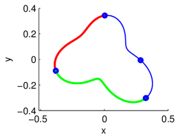
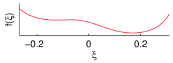
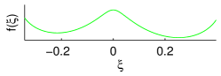
Figure 1: Interface split into segments (ends marked with $\circ$), with two segments drawn bold, and their local representations.

That is, assume there exists a in interval of $s^{\prime}\subseteq s$ and mapping $\mathcal{M}$ such that

$$\mathcal{M}\gamma=(\xi,f(\xi))$$ (2)

with $\gamma:=\Gamma(s^{\prime})$. We call this representation, $\mathcal{M}\gamma:=\gamma_{\text{loc}}$, the segment in local coordinates, as opposed to $\gamma$, which we will refer to the segment in global coordinates. The mapping will be composed of a translation, $\mathbf{b}$, and a unitary rotation, $\mathcal{T}$, of some angle $\theta$. We define this mapping and its inverse as

$$\mathcal{M}\mathbf{x}:=\mathcal{T}(\theta)\mathbf{x}+\mathbf{b}$$ (3)

$$\mathcal{L}\mathbf{x}:=\mathcal{M}^{-1}\mathbf{x}=\mathcal{T}(-\theta)(\mathbf{x}-\mathbf{b}),$$ (4)

for any $\mathbf{x}\in\mathbb{R}^{2}$. The inverse mapping $\mathcal{L}$ will naturally play the role of transforming the segment from local to global coordinates, i.e.

$$\mathcal{L}:\,\,\gamma_{\text{loc}}\rightarrow\gamma.$$

Now we proceed to providing an equation for the time evolution of each segment. Differentiate the transformation (3) to obtain

$$\frac{\mathrm{d}}{\mathrm{d}t}\mathcal{M}\gamma=\begin{bmatrix}\left(\frac{\mathrm{d}}{\mathrm{d}t}\mathcal{M}\gamma\right)_{1}\\ \left(\frac{\mathrm{d}}{\mathrm{d}t}\mathcal{M}\gamma\right)_{2}\end{bmatrix}=\begin{bmatrix}\frac{\mathrm{d}\xi}{\mathrm{d}t}\\ \frac{\partial f}{\partial t}+\frac{\mathrm{d}\xi}{\mathrm{d}t}\frac{\partial f}{\partial\xi}\end{bmatrix}.$$

Hence, we have

$$\frac{\partial f}{\partial t}+\left(\frac{\mathrm{d}}{\mathrm{d}t}\mathcal{M}\gamma\right)_{1}\frac{\partial f}{\partial\xi}=\left(\frac{\mathrm{d}}{\mathrm{d}t}\mathcal{M}\gamma\right)_{2}$$

which we may write more conveniently as

$$\frac{\partial f}{\partial t}+\left(\frac{\mathrm{d}}{\mathrm{d}t}\mathcal{M}\gamma\right)\cdot\left[\frac{\partial f}{\partial\xi},\quad-1\right]=0.$$ (5)

We shall consider first the case where the mapping parameters $\theta$ and $\mathbf{b}$ are both constant and then, in Section 2.8 we present an extension where we have them as time dependent functions, $\theta(t)$ and $\mathbf{b}(t)$.

For the first case it is evident that

$$\frac{\mathrm{d}}{\mathrm{d}t}\mathcal{M}\gamma= \mathcal{J}(\mathcal{M}\gamma)\frac{\mathrm{d}\gamma}{\mathrm{d}t}$$

$$= \mathcal{T}(\theta)\mathbf{u}(\gamma,t),$$

where $\mathcal{J}$ is the Jacobian and we have used the interface ODE (1). Then we have the segment advection PDE given by

$$\frac{\partial f}{\partial t}+v(\gamma,t)\frac{\partial f}{\partial\xi}=w(\gamma,t),$$ (6)

where we have introduced $\mathcal{T}(\theta)\mathbf{u}(\gamma,t)=:(v,w)$. This is an advection-type PDE with a source term. Note that the parameters $v$ and $w$ depend on the interface location, so the PDE is non-linear. In Section 2.1 we give an explicit and an implicit method to treat this PDE numerically in a simple manner.

2.1 Segment discretization

We now present numerical methods for treating the segment advection equations (6). There are two primary issues to address. First, as previously noted, we deal with non-linear equations. However, these are hyperbolic – in quasi-linear form – and the non-linearity presents no major concern.

The second complication concerns boundary conditions and is more interesting: there are no boundary conditions at the ends of each segment end if the interface is closed. We have decomposed the interface into segments, which leaves us with the requirement that segments match where they meet and that smoothness is preserved there. It is then natural that we devise a domain decomposition method that solves the segment advection equation concurrently in time for all segments.

We discretize the segment functions, $f(\xi)$ on uniform grids in $\xi$, e.g. $\xi_{i}=a+i\Delta\xi$. This constitutes a simplification over other methods – we can use difference formulas over 1D uniform grids for our numerical treatment of the segment advection PDE as well as all invariant interface quantities that we may need (such as curvature, normals, quadrature formulas etc.).

The convective field, $\mathbf{u}(\cdot,t)$, may be an explicit function, as in our test problems later in this paper. We also give examples later where $\mathbf{u}$ is a functional over the interface (in a boundary integral method), and, finally, a numerical solution operator to the incompressible Navier Stokes equations. From the point of view of the interface tracking method, $\mathbf{u}(\cdot,t)$ is a black box that orders a convective field to the grid function on $\xi$.

In anticipation of these more general coefficient operators it is sensible to introduce Strang splitting for the pair $(f,\mathbf{u})$: Let $\mathbf{u}$ be discretized on staggered time levels, i.e. that

$$\begin{split}\mathbf{u}^{n-1/2}\rightarrow\mathbf{u}^{n+1/2}\text{ using }f^{n}\text{ and}\\ f^{n}\rightarrow f^{n+1}\text{ using }\mathbf{u}^{n+1/2}.\end{split}$$ (7)

It is clear for linear systems that this method maintains second order accuracy, provided second order accurate time step schemes for $f$ and $\mathbf{u}$ (if $\mathbf{u}$ is governed by a differential equation).

2.2 Lax-Wendroff method for segments

For the explicit method we will derive a Lax-Wendroff method with central difference approximations in space (see e.g. the textbook by LeVeque [26]). The same method was used by Tornberg et. al. in the segment projection method [24], and we present it here for completeness. Consider

$$f_{t}+v(\mathbf{x}(t),t)f_{\xi}=w(\mathbf{x}(t),t)$$ (8)

and let $\Delta t$ represent the time step. Note that at a particular point in time, $v$ and $w$ are functions of $\xi$. We have a Taylor expansion

$$f(t+\Delta t,\xi)=f(t,\xi)+\Delta tf_{t}(t,\xi)+\frac{\Delta t^{2}}{2}f_{tt}(t,\xi)+\dots$$

where the task is to replace time-derivatives with derivatives in space. From (8) we have

$$f_{t}=w(\mathbf{x},t)-v(\mathbf{x},t)f_{\xi}.$$

This implies that

$$f_{tt} =(w(\mathbf{x},t)-v(\mathbf{x},t)f_{\xi})_{t}$$

$$=\frac{\mathrm{d}}{\mathrm{d}t}w(\mathbf{x},t)-f_{\xi}\frac{\mathrm{d}}{\mathrm{d}t}v(\mathbf{x},t)-v(\mathbf{x},t)f_{t\xi}$$

$$=\frac{\mathrm{d}}{\mathrm{d}t}w(\mathbf{x},t)-f_{\xi}\frac{\mathrm{d}}{\mathrm{d}t}v(\mathbf{x},t)-v(\mathbf{x},t)(w(\mathbf{x},t)-v(\mathbf{x},t)f_{\xi})_{\xi}$$

$$=\frac{\mathrm{d}}{\mathrm{d}t}w(\mathbf{x},t)-f_{\xi}\frac{\mathrm{d}}{\mathrm{d}t}v(\mathbf{x},t)-v(\mathbf{x},t)\left(\frac{\mathrm{d}}{\mathrm{d}\xi}w(\mathbf{x},t)-f_{\xi}\frac{\mathrm{d}}{\mathrm{d}\xi}v(\mathbf{x},t)+v(\mathbf{x},t)f_{\xi\xi}\right).$$

Plugging into the Taylor expansion gives the semi-discrete scheme

$$f(\xi,t+\Delta t) =f(\xi,t)+\Delta t\left(w(\mathbf{x},t)-v(\mathbf{x},t)f_{\xi}\right)+$$

$$+\frac{\Delta t^{2}}{2}v(\mathbf{x},t)\left(-\frac{\mathrm{d}}{\mathrm{d}\xi}w(\mathbf{x},t)+f_{\xi}\frac{\mathrm{d}}{\mathrm{d}\xi}v(\mathbf{x},t)+v(\mathbf{x},t)f_{\xi\xi}\right)+$$

$$+\frac{\Delta t^{2}}{2}\left(\frac{\mathrm{d}}{\mathrm{d}t}w(\mathbf{x},t)-f_{\xi}\frac{\mathrm{d}}{\mathrm{d}t}v(\mathbf{x},t)\right).$$ (9)

Recall that $\mathbf{x}$ corresponds to $f$ via the mapping $\mathcal{M}$.

For the discretization in space we introduce the usual difference operators $D_{0}$, $D_{-}$ and $D_{+}$, i.e. for some grid function $q_{i}$ on the $\xi$-grid, discrete derivative approximations are obtained via

$$(D_{0}q)_{i}=\frac{1}{2\Delta\xi}(q_{i+1}-q_{i-1}),\quad(D_{-}q)_{i}=\frac{1}{\Delta\xi}(q_{i}-q_{i-1}),\quad(D_{+}q)_{i}=\frac{1}{\Delta\xi}(q_{i+1}-q_{i}).\quad$$

Despite the fact that this Lax-Wendroff method uses centered difference approximations to discretize a convective equation, it is stable provided that the CFL condition is satisfied [26]. We note that we will maintain formal second order accuracy even if the time derivatives in the last terms are only approximated to first order and, hence, we use a forward approximation here by taking an Euler step to get an approximate interface location where the coefficients can be reevaluated:

$$f^{*}=f^{n}+\Delta t(w(\mathbf{x}^{n},t^{n})+v(\mathbf{x}^{n},t^{n})D_{0}{f^{n}})$$ (10)

so that

$$f^{n+1}=f^{*} +\frac{\Delta t^{2}}{2}v(\mathbf{x}^{n},t^{n})\left(-D_{0}w(\mathbf{x}^{n},t^{n})+(D_{0}v(\mathbf{x}^{n},t^{n}))(D_{0}f^{n})+v(\mathbf{x}^{n},t^{n})D_{+}D_{-}f^{n}\right)-$$

$$+\frac{\Delta t^{2}}{2}\left(\frac{w(\mathbf{x}^{*},t^{n+1})-w(\mathbf{x}^{n},t^{n})}{\Delta t}-\frac{v(\mathbf{x}^{*},t^{n+1})-v(\mathbf{x}^{n},t^{n})}{\Delta t}D_{0}f^{n}\right).$$ (11)

We emphasize that the evaluation of the coefficients are typically done in global coordinates, i.e. via the mapping and its inverse. See Section 2.7 for a summary of the method. As previously noted, one may often (depending on how $\mathbf{u}$ is computed) want to apply Strang splitting (7), i.e. taking all time levels above to $t^{n+1/2}$.

2.3 How to close the system

It remains to discuss the how to couple the segments together. With an equation of the form (8) it is clear that information will be propagated along characteristics across segment boundaries. In the language of numerical methods for conservation laws, any difference approximation must then look upwind across to the adjacent segment at any boundary where there are incoming characteristics.

In our proposed method above, centered differences are used. The Lax-Wendroff method introduces a diffusive term which stabilizes it (see LeVeque [26, pp. 100-102]). Numerically, we then have information propagating in both directions at each segment boundary. In practice this means that we need ghost points at each end of each segment.

To evaluate $D_{0}$ we can exchange ghost values at time $t^{n}$. Note that adjacent segments have different parametrization, so one may need to construct a small interpolant from the end of the adjacent segment in order to evaluate the ghost point, see Figure 2. That is, let $(\xi_{k},f_{k}(\xi))$ be the local representation of segment $k$ (or part of). To view this segment in the coordinate frame of segment $j$, simply use the mappings: $(\xi_{j},f_{j}(\xi))=\mathcal{M}_{j}\mathcal{L}_{k}(\xi_{k},f_{k}(\xi))$. With this exchange of ghost points, the system is closed in the sense that the concurrent updates of all segments is equivalent to (1).

From a theoretical point of view it is important that there exists a finite overlap between segments (for the manifold properties to exist). That is, one must be able to go from one segment to another via the global coordinate representation. If this property is not satisfied, it becomes impossible to evaluate the ghost points as discussed above. Thus, it will be necessary as the interface deforms to expand and/or contract the domain of definition of some, or all, segments. However, growing a segment involves an adjacent segment in the same fashion as the ghost points. We emphasize that this is handled on a regular grid and, thus, does not pose a particular difficulty (as one may view the point distribution problem in front tracking methods).

Figure 2: Ghost point $(\times)$, evaluated from part of adjacent segment (solid line), with local segment grid function (dots).

2.4 Implicit methods for segment advection

The natural framework for treating hyperbolic PDEs, including the segment advection equation $f_{t}+v(\xi,t)f_{\xi}=w(\xi,t)$, are explicit finite volume methods (to which the Lax-Wendroff method may be said to belong). None the less, implicit methods are often proposed for interface tracking problems, with enhanced time-stability in mind.

As a motivating example, consider a multi-phase flow application. A common approach is to split the tasks of interface tracking and solving flow equations into interleaving steps. It is evident that numerical schemes for both interface tracking and bulk flow should be governed by CFL-type time-step restrictions, and indeed, a wealth of numerical methods exist with this property. However, it has been observed, e.g. in Peskin and Tu [27], LeVeque and Lee [8], Le et. al. [10] and Li and Ito [9, p. 226], that this split leads to a stiff system that is no longer stable in the CFL regime. Thus implicit methods are advocated to maintain the stability region.

A time-discrete implicit method may take the form

$$f^{n+1}=\mathcal{F}(f^{n+1},f^{n},t,\dots),$$

which naturally suggests Newton- or fix-point iteration methods to solve for $f^{n+1}$. In our framework it is natural to iterate the segments concurrently, in lieu of the coupling between adjacent segments (previous section). Let the leading super-index of $f^{k,m}$ refer to segment $k$ in the collection that constitutes the interface, and let the latter index denote time-level or iteration count. Then an iterative method is outlined as follows: Until convergence, $\|f^{k,(i+1)}-f^{k,(i)}\|<\epsilon,\forall k$, do

1. Exchange ghost points between all adjacent segments,

2. For each segment, $k$, compute new iterate, e.g.

   $$f^{k,(i+1)}\leftarrow\mathcal{G}(f^{k,(i)},f^{k,n},\mathcal{F},\dots),$$

   for some $\mathcal{G}$ that defines the iterative procedure,

and let $f^{k,n+1}$ be the converged iterate for each segment.

2.4.1 Crank-Nicholson (CN) method for segments

We now proceed to a concrete method along the lines of the previous section. In [8] and [10] a Crank-Nicholson method for (1) is suggested,

$$\mathbf{x}^{n+1}=\mathbf{x}^{n}+\frac{\Delta t}{2}\left(\mathbf{u}(\mathbf{x}^{n},t^{n})+\mathbf{u}(\mathbf{x}^{n+1},t^{n+1})\right),$$

together with an iterative method for solving this nonlinear system. This suggests that if we have

$$\frac{\mathrm{d}f}{\mathrm{d}t}=Q(t)f(\mathbf{x},t)+P(t)$$ (12)

where $Q$ is (possibly) a spatial differential operator, we should study methods of the form

$$f^{n+1}=\mathcal{F}(f^{n+1},f^{n}):=f^{n}+\frac{\Delta t}{2}\left(Q^{n}f^{n}+Q^{n+1}f^{n+1}+P^{n}+P^{n+1}\right).$$ (13)

From (6) we get a semi-discrete equation on the form (12) with

$$Q=-v(\mathbf{x},t)D_{0}$$

$$P=w(\mathbf{x},t).$$

We use the following iterative procedure to solve (13) for $f^{n+1}$, which follows the approach presented in [8]:

1. Initial guess, $f^{(0)}=f^{n}-\Delta tv^{n}D_{0}f^{n}+\Delta tw^{n}$. Set $i=0$.

2. Evaluate $\mathbf{u}^{(i)}$. This might involve solving flow equations (or more).

3. Exchange ghost points between all adjacent segments.

4. Evaluate the residual,

   $$g(f^{(i)})=f^{(i)}-f^{n}-\frac{\Delta t}{2}(-v^{n}(t^{n})D_{0}f^{n}-v^{(i)}(t^{n+1})D_{0}f^{(i)}+$$ (14)

   $$+w^{n}(t^{n})+w^{(i)}(t^{n+1}))$$

5. If $\|g(f^{(i)})\|<\epsilon$ then terminate and set $f^{n+1}=f^{(i)}$. Else increment $i$, compute new $f^{(i)}$ and go to step 2. Computing the next iterate should be done cleverly – LeVeque[8] suggests a BFGS or SR1 method.

The BFGS method amounts to a Newton-type iteration where, after applying the Sherman-Morrison formula, an approximation to the inverse Jacobian (denoted $B$) is computed concurrently with the solution to the system (from [9, Sec. 10.2.5]):

$$f^{(i+1)}=f^{(i)}-B_{n}^{(i)}g(f^{(i)})$$

$$B_{n}^{(i+1)}=B_{n}^{(i)}+\frac{\mu_{i}s_{i}s_{i}^{T}-s_{i}y_{i}^{T}B_{i}^{n}-B_{n}^{(i)}y_{i}s_{i}^{T}}{s_{i}^{T}y_{i}},$$

where

$$s_{i}:=-B_{n}^{(i)}g(f^{(i)}),\quad y_{i}:=g(f^{(i+1)})-g(f^{(i)}),\quad\mu_{i}:=1+\frac{y_{i}^{T}B_{n}^{(i)}y_{i}}{s_{i}^{T}y_{i}}.$$

Here, as in the explicit method, the coefficients $v^{(i)}$ and $w^{(i)}$ are evaluated from $f^{(i)}$ in global coordinates via the mapping (3) and its inverse. We have found that given the initial guess computed from the previous time step, this iterative method is reliably convergent in two to five iterations, which is well within the practical range, even if $\mathbf{u}$ is expensive to evaluate (see Section 5.4 for more remarks on this).

In practice, we have found the iterative method to relax the CFL time step restriction present in the explicit method. However, arbitrarily large time steps can not be taken, in part due to the requirement that the segments maintain a finite overlap throughout the iterative procedure (for the evaluation of ghost points). More remarks on the stability of these methods when applied to the Navier-Stokes equations are given in Section 5.4.

2.5 Error analysis

The truncation error in each of the methods above is $\mathcal{O}(\Delta\xi^{2})+\mathcal{O}(\Delta t^{2})+\mathcal{O}(N_{t}\Delta\xi^{p})$, where $p$ is the order of the interpolation method used to evaluate the ghost points from adjacent segments and $N_{t}:=T/\Delta t$ is the number of time steps taken. One can show, by constructing a partition of unity, that the accuracy order in the interface itself is equal to the order obtained for each segment (i.e. second order).

2.6 Finding and maintaining segments

An interesting question naturally arises from the assumptions on our method: does there exist a decomposition of a curve into segments, and if so, how do we find it and the mapping parameters in (3)?

In a continuous setting it is clear from elementary calculus that this partitioning exists provided sufficient regularity on $\Gamma$. However, the curve may have, or develop, a interval with arbitrary curvature. This provides a problem in the discrete setting because it implies an upper bound on the curvature that can be reasonably resolved with a given segment discretization. There is also the question of optimality: partitioning the interface with as few segments as possible. We do not address the latter issue, because there is no benefit for our method in having very few segments.

We will also give some remarks on how to verify that the segments, as the interface deforms, remain valid (i.e. single valued). But fist the partitioning problem.

2.6.1 Partitioning the interface

Given a discrete plane curve $(x_{i},y_{i})$, $i=1\dots N$, the task is to split the index space into intervals that are monotonous with respect to some basis vector. To be precise, consider an interval $i=p,p+1,\dots p+M$ and associate with this segment a mapping (3), i.e. $\mathcal{M}:(x,y)\rightarrow(\xi,f)$. The segment of $\mathbf{x}$ from $p$ to $p+M$ is strictly monotonous with respect to the direction defined by $\mathcal{M}$ if $\xi_{i}$, $i=1,\dots,M$, is strictly monotonous.

A large body of work exists in the field of image processing that aims to reconstruct geometric features from image data with robust methods. Some related work to our partitioning problem can be found in [28, 29, 30, 31]. However, we were not able to find a suitable method there or in the references therein.

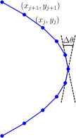
Figure 3: Winding angle, positive with respect to the orientation indicated.

The method we propose uses the winding angle, $\Delta\theta_{i}$, as defined in Figure 3, and a cumulative winding angle,

$$\theta_{I}:=\sum_{i\in I}^{M}\Delta\theta_{i}.$$

Then we may say that an interval $\varsigma=\{i=p\dots p+M\}$ is monotonous if

$$\max\theta_{\varsigma}-\min\theta_{\varsigma}<\pi.$$ (15)

In practice it makes sense to have segments that sweep less than the maximal winding angle, $\pi$. So we we iterate over the curve, $(x_{i},y_{i})$ from some starting index $p$ and break to a new segment when we encounter an $M$ such that $\max\theta_{\varsigma}-\min\theta_{\varsigma}\geq\eta$. Here $\eta<\pi$ is a parameter that affects how many segments we obtain, e.g. $\eta=\pi/2$ gives a partitioning of a circle into four segments.

2.6.2 Segment validity

It is clear that, if the interface deforms sufficiently, the collection of segments initially constructed may fail to correctly represent the interface. That is, given an interface, it may not be possible to satisfy the constraint of having single-valued segment functions with a given number of segments. Hence, to handle cases with large deformation, we need to monitor the segment description and recompute the partition if necessary. We choose to put an upper bound on the variation of the discrete segment function,

$$|f_{n+1}-f_{n}|\leq K|\xi_{n+1}-\xi_{n}|,$$

where $K$ is a parameter. Also, it is sensible to require that the segments be at least $d$ grid-points long. If the interface develops a point of very high curvature, the length condition will suggest that a finer grid is needed to resolve the interface. Typical values may be $K=5$ and $d=20$.

2.7 Summary of method

Now we summarize the proposed method:

Time step (explicit method)

To advect the interface from $t_{n}$ to $t_{n+1}$ do,

1. Exchange ghost points between all segments, see Section 2.3.

2. For each segment (individually): evaluate coefficients $v(\mathbf{x}^{n},t^{n}),w(\mathbf{x}^{n},t^{n})$ by using the transformation to global coordinates. Then, take Euler step (10) to obtain $f^{*}$, and reevaluate the coefficients $v(\mathbf{x}^{*},t^{n+1}),w(\mathbf{x}^{*},t^{n+1})$. Finally compute the correction step (11), getting $f^{n+1}$. See Section 2.2.

3. Verify that segments are valid, see Section 2.6.2, and possibly grow/contract segments so that the evaluation of ghost points possible in the next step.

4. If segments are not valid, compute a new partitioning (Section 2.6.1).

The implicit method is proceeds similarly, the key difference being that item two (2.) above is replaced by the iterative procedure given in Section 2.4.1.

2.8 Velocity field decomposition and time-dependent mapping

Finally, before presenting numerical results and applications, we make an extension of the method, where the mapping parameters are allowed to vary over time. Is essence, this poses the method hitherto presented in moving reference frames.

We see in a number of interface tracking applications that there often exists large scale deformations that translate the interface or rotate it as a solid body – physical flows are e.g. often directional with some length scale. These kinds of motion may be easily treated in our method by simply updating the segment mapping parameters (the offset $\mathbf{b}$ and the rotation $\theta$), whereas interface deformations are treated by solving the advection PDE (5), see Section 3 for numerical results. To make use of this, consider a decomposition of the velocity field $\mathbf{u}$,

$$\mathbf{u}(\mathbf{x},t)=\mathbf{u}_{\text{trans}}+\bar{\omega}\times(\mathbf{x}-\mathbf{b})+\mathbf{u}_{\text{rest}}(\mathbf{x},t),$$ (16)

where $\bar{\omega}=\omega\hat{\mathbf{z}}$. Since we know $\mathbf{u}_{i}=(v_{i},w_{i})$ at many points $\mathbf{x}_{i}$ we may solve for the decomposition parameters $\omega$ and $\mathbf{u}_{\text{trans}}=(v_{b},w_{b})$ in a least squares sense:

$$\begin{bmatrix}(-y_{1}+y_{b})&1&0\\ (-y_{2}+y_{b})&1&0\\ \vdots&\vdots&\vdots\\ (x_{1}-x_{b})&0&1\\ (x_{2}-x_{b})&0&1\\ \vdots&\vdots&\vdots\end{bmatrix}\begin{bmatrix}\omega\\ v_{b}\\ w_{b}\end{bmatrix}=\begin{bmatrix}v_{1}\\ v_{2}\\ \vdots\\ w_{1}\\ w_{2}\\ \vdots\end{bmatrix}$$ (17)

where $\mathbf{b}=(x_{b},y_{b})$.

With this we return to (5), calculating $\frac{\mathrm{d}}{\mathrm{d}t}\mathcal{M}\gamma$ where $\frac{\mathrm{d}\theta}{\mathrm{d}t}=\omega$ and $\frac{\mathrm{d}\mathbf{b}}{\mathrm{d}t}=\mathbf{u}_{\text{trans}}$ in order to obtain a PDE similar to (6). We get

$$\frac{\mathrm{d}}{\mathrm{d}t}\mathcal{M}(\mathbf{x})= \mathcal{T}(\theta)\frac{\mathrm{d}\mathbf{x}}{\mathrm{d}t}+\frac{\mathrm{d}\mathbf{b}}{\mathrm{d}t}+\frac{\mathrm{d}\mathcal{T}(\theta)}{\mathrm{d}t}\mathbf{x}$$

$$= \mathcal{T}(\theta)\mathbf{u}(\mathbf{x},t)+\mathbf{u}_{\text{trans}}+\frac{\mathrm{d}\mathcal{T}(\theta)}{\mathrm{d}t}\mathbf{x}$$

Differentiating the rotation operator is straight-forward,

$$\frac{\mathrm{d}}{\mathrm{d}t}\mathcal{T}(\theta)= \begin{bmatrix}-\frac{\mathrm{d}\theta}{\mathrm{d}t}\sin(\theta)&-\frac{\mathrm{d}\theta}{\mathrm{d}t}\cos(\theta)\\ \frac{\mathrm{d}\theta}{\mathrm{d}t}\cos(\theta)&-\frac{\mathrm{d}\theta}{\mathrm{d}t}\sin(\theta)\end{bmatrix}$$

$$= \,\,\omega\begin{bmatrix}\cos(\pi/2+\theta)&-\sin(\pi/2+\theta)\\ \sin(\pi/2+\theta)&\cos(\pi/2+\theta)\end{bmatrix}$$

$$= \,\,\omega\mathcal{T}(\pi/2+\theta).$$

Using this we get

$$\frac{\mathrm{d}}{\mathrm{d}t}\mathcal{M}(\mathbf{x})=\mathcal{T}(\theta)\mathbf{u}(\mathbf{x},t)+\mathbf{u}_{\text{trans}}+\omega\mathcal{T}(\pi/2+\theta)\mathbf{x}.$$ (18)

Inserting this into (5) gives a PDE, of the same type as (6), for the segment dynamics in the case when the velocity field decomposition (16):

$$\frac{\partial f}{\partial t}+\big{(}\mathcal{T}(\theta)\mathbf{u}_{\text{rest}}+\mathbf{u}_{\text{trans}}+\omega\mathcal{T}(\pi/2+\theta)\gamma\big{)}\cdot\left[\frac{\partial f}{\partial\xi}\quad-1\right]=0.$$ (19)

The discretization of this PDE fits naturally into the explicit method summarized above, with two additions. First, apply Strang splitting (7) to obtain a second order accurate method. Secondly, the mapping parameters are updated before the coefficients $(v,w)$ are reevaluated,

$$\theta^{n+1}=\theta^{n}+\Delta t\omega$$

$$\mathbf{b}^{n+1}=\mathbf{b}^{n}+\Delta t\mathbf{u}_{\text{trans}}.$$

3 Numerical results for interface tracking

Here we provide numerical results for the pure interface tracking problem. So as to not introduce any new discretization errors, we let the convective velocity field be given by a closed expression (as opposed to computing an approximate solution to e.g. Navier Stokes equations):

$$\mathbf{u}_{I}(\mathbf{x},t)=\cos(\pi t)\big{(}-\cos(x_{i}-\pi/2)\sin(x_{2}-\pi/2)\quad\cos(x_{2}-\pi/2)\sin(x_{1}-\pi/2)\big{)}$$ (20)

$$\mathbf{u}_{II}(\mathbf{x},t)=\big{(}\sin(\pi x)^{2}\sin(2\pi y)\quad-\sin(\pi y)^{2}\sin(2\pi x)\big{)}$$ (21)

An example of a computation with $\mathbf{u}=\mathbf{u}_{II}$ can be seen in Figure 4. The curvature of the interface is known to to be difficult to compute, even to “eye norm” accuracy. It is even the case with many methods that some kind of filtering is needed to get acceptable curvature results, though this is not generally discussed. In Figure 4, we also show the interface curvature at different times. The two sharp peaks are well captured, without any oscillations, and there are no visible artifacts at the segment boundaries. We compute curvature in local coordinates, via

$$\kappa(\xi)=\frac{f^{\prime\prime}(\xi)}{(1+f^{\prime}(\xi)^{2})^{3/2}},$$ (22)

as discretized with the usual centered difference approximations.

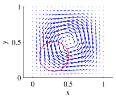
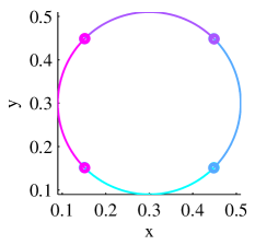
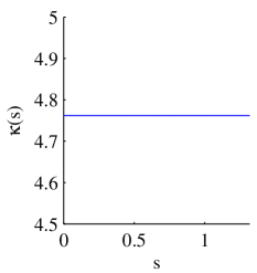
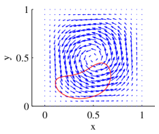
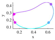
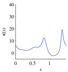
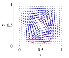
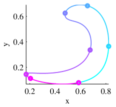
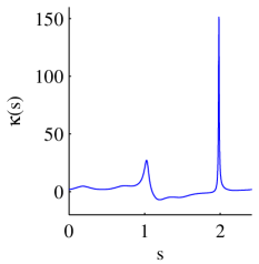
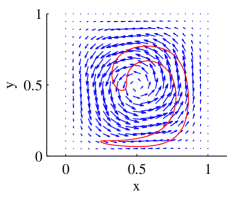
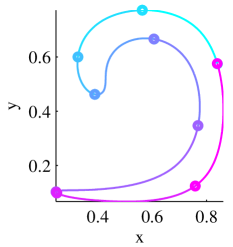
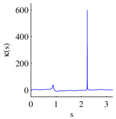
Figure 4: Interface and curvature at times $t=0,\,0.2,\,0.6,\,0.9$, where the convective velocity field is given by (21). The circles mark (middle column) the segment boundaries.

For testing numerical convergence we construct test cases that have an analytical solution. The convective field $\mathbf{u}_{I}$ oscillates so that, at $t=1$, the interface is returned to its initial configuration, which we take to be a circle. In Figure 5 we present convergence results for both the interface location and its curvature as the grid is refined, with the explicit (LaxW) method. The time step is refined so that the ratio $\Delta\xi/\Delta t=2$ is kept constant. We see the expected second order convergence in both time and space for the interface, in $\|\mathbf{x}(T)-\mathbf{x}(0)\|_{\infty}$. In Figure 6 we give similar results for the implicit (CN) method.

3.1 Convergence in curvature

Also in Figure 5, to substantiate our claim that the interface curvature is well captured by our method, we give convergence results for curvature. Here we see first order convergence in $\|\kappa(s,T)-1/r\|_{\infty}$ and close to second order convergence in $\|\kappa(s,T)-1/r\|_{l^{2}}$. That the 2-norm convergence is substantially higher than in $\infty$-norm tells us that the first order errors are highly localized. These results are with the LaxW method and we wish to emphasize that no filtering or smoothing of any kind were used to obtain them. Together with the second order convergence of the interface in $\infty$-norm, we take these curvature convergence results as strong endorsement of the accuracy of the proposed method. In particular, the domain-decomposition approach seems vindicated.

With the CN method we were not able to get equally convincing convergence results for the curvature. Still, in Figure 6, we have first order convergence of the curvature in 2-norm (in $\infty$-norm we have convergence, but of order $<1$).

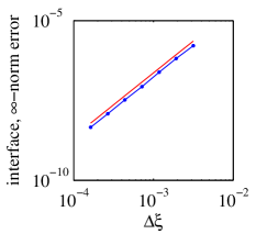
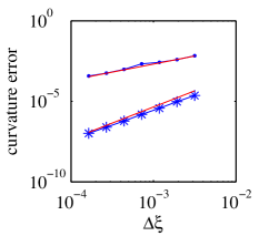
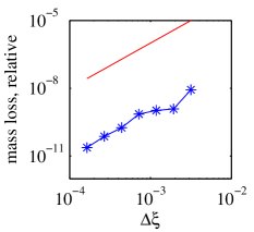
Figure 5: Explicit (LaxW) method. Left: Convergence of interface in $\infty$-norm as grid is refined, with $\mathbf{u}=\mathbf{u}_{I}$ (Eq. (20)), at $t=1$. Middle: Convergence of interface curvature in ($\cdot$) $\infty$- and ($*$) $2$-norm. Right: Convergence in relative mass loss (solid line denotes second order convergence).

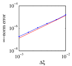
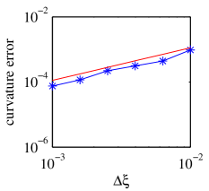
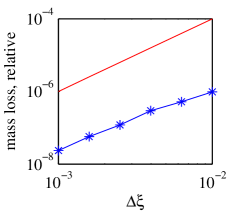
Figure 6: Implicit (CN) method. Left: Convergence of interface in $\infty$-norm as grid is refined, with $\mathbf{u}=\mathbf{u}_{I}$. Middle: Convergence of interface curvature in ($*$) $2$-norm. Right: Convergence in relative mass loss (solid line denotes second order convergence).

3.2 Mass, or area, conservation

There is no inherent mass conservation in our method. On the other hand, there is no reason to expect it to suffer from poor mass conservation in the same way as level set methods are known to do.

In Figures 5 and 6 (right column) we give mass loss results as the interface is refined, for the explicit and implicit method. That is, we compute the mass loss as a relative measure, via $(\text{mass}(0)-\text{mass}(T))/\text{mass}(0)$ where the mass is simply computed as the area of the polygon enclosed by the interface.

We note here that the mass loss shows second order convergence as the interface is refined, and that the constant is very small – several orders of magnitude below unity.

3.3 Dynamic mapping parameters

Finally, before we develop applications, we give numerical results for the extended method in Section 2.8, where the mapping parameters vary. Again with the oscillating circle case $\mathbf{u}=\mathbf{u}_{I}$, we have second order convergence in the interface in $\infty$-norm, first order convergence in curvature and second order convergence in the mass conservation, see Figure 7. In Figure 8 we give results where the interface is advected in a pure rotation velocity field, as is a common test case for interface tracking methods. A notable characteristic of our method is that, aside from initialization errors, there are no numerical errors in this computation, because of the velocity field decomposition.

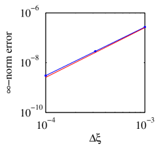
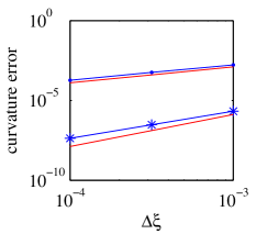
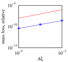
Figure 7: Explicit (LaxW) method, with velocity field decomposition (Section 2.8). Left: Convergence of interface in $\infty$-norm as grid is refined, with $\mathbf{u}=\mathbf{u}_{I}$. Middle: Convergence of interface curvature in ($\cdot$) $\infty$- and ($*$) $2$-norm. Right: Convergence in relative mass loss (solid line denotes second order convergence).

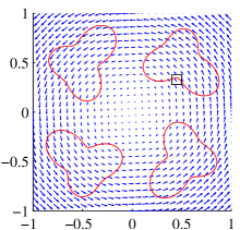
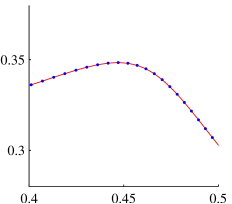
Figure 8: Left: Interface at four times, and pure rotation velocity field. Left: Close up of boxed region in left figure, with interface at $t=0$ as solid red line, and interface at $t=2\pi$ as dots. These are indistinguishable.

4 Boundary integral method for Stokes in 2D

When applicable, boundary integral methods are often efficient. Here we give a boundary integral formulation for Stokes flow in 2D using our method. This illustrates some important simplifications that arise when using our method.

For an introduction to the field of boundary integral methods for viscous flow, we refer to the textbooks Pozrikids [32] and Kim and Karrila [33], as well as a more recent survey paper by Pozrikidis [34].

Using the so called single layer formulation, the velocity at any point, $x_{0}\in\Omega\subset\mathbb{R}^{n}$, can be evaluated as

$$u_{i}(x_{0})=\int_{\Gamma}G_{ij}(x,x_{0})q_{j}(x)\mathrm{d}S(x),$$ (23)

where $G_{ij}$ is a Greens function (fundamental solution) called the Stokeslet, and $q_{j}$ is a source density on the interface. Here we consider a free space problem in $\mathbb{R}^{2}$. Then the Stokeslet is given by

$$G_{ij}(x,x_{0})=-\delta_{ij}\log(r)+\frac{\hat{x}_{i}\hat{x}_{j}}{r^{2}},$$

where $\hat{x}=x-x_{0}$, $r=|\hat{x}|$ and $\delta_{ij}$ is the Kronecker symbol. There remains only to compute the densities $q_{j}$, which in general requires solving a (full) linear system. However, in the case where the viscosity inside is equal to the viscosity outside of the interface, one obtains

$$q_{j}(s)=-\frac{1}{4\pi\mu}f_{j}(s),$$

where $s$ parametrizes $\Gamma$ and $\mu$ is the viscosity. These results were given in [35]. The force acting on the interface is simply

$$f_{j}(s)=\sigma\kappa(s)\hat{n}_{j}(s),$$

where $\sigma$ is the coefficient of surface tension, $\kappa$ is the curvature and $\hat{n}_{j}$ are the unit normals. In terms on non-dimensional variables, we write

$$q_{j}(s)=-\frac{1}{4\pi\text{Ca}}\kappa(s)\hat{n}_{j}(s),$$

where $\text{Ca}:=\frac{U\mu}{\sigma}$ is known as the capillary number (for some typical velocity scale $U$).

Now we pose the evaluation of (23) in the setting of our segments. By definition we have that any integral over the interface can be split into a sum of integrals over the segments $\gamma_{i}$,

$$\int_{\Gamma}g(s)\mathrm{d}s =\sum_{i}\int_{\gamma_{i}}\tilde{g}(\xi)\mathrm{d}\xi_{f}$$ (24)

$$=\sum_{i}\int_{\gamma_{i}}g(s(\xi))\sqrt{1+f^{\prime}(\xi)^{2}}\mathrm{d}\xi.$$

In order to perform this change of variables in (23) from a global parametrization, $s$, to local variables $(\xi,f(\xi))$ we note a few invariant properties of the integrand. First, the curvature is a geometric invariant, so instead of computing $\kappa(s)$ we can compute it in local coordinates directly, as given by (22). Similarly, for the normal vectors we directly compute

$$\hat{n}(\xi)=[f^{\prime}(\xi)\quad-1].$$

Finally, note that the global-to-local mapping, $\mathcal{M}$ (cf. Eq. (3)) is distance preserving. Hence, we directly express the Stokeslet in local coordinates

$$G_{ij}(\xi,f(\xi),x_{0})=-\delta_{ij}\log(r)+\frac{\tilde{\mathbf{x}}_{i}\tilde{\mathbf{x}}_{j}}{r^{2}},$$

where $\tilde{\mathbf{x}}:=(\xi,f(\xi))-\mathcal{M}x_{0}$ and $r=\|\tilde{\mathbf{x}}\|$. For a point $x_{0}$ away from the interface, using the inverse mapping (4), we have that

$$u(x_{0}) =-\frac{1}{4\pi\mu}\sum_{k}\mathcal{L}_{k}\int_{\gamma_{k}}\kappa(\xi)G_{ij}(\xi,f(\xi),x_{0})\hat{n}_{j}(\xi)\mathrm{d}\xi_{f}$$

$$=-\frac{1}{4\pi\mu}\sum_{k}\mathcal{L}_{k}\int_{\gamma_{k}}\frac{f^{\prime\prime}(\xi)}{1+f^{\prime}(\xi)^{2}}G_{ij}(\xi,f(\xi),x_{0})\hat{n}_{j}(\xi)\mathrm{d}\xi$$ (25)

$$=-\frac{1}{4\pi\mu}\sum_{k}\mathcal{L}_{k}\int_{\gamma_{k}}q^{f}_{j}(\xi)G_{ij}(\xi,f(\xi),x_{0})\mathrm{d}\xi.$$

These integrals are naturally discretized on the segment grids, where the start of the integration interval, denoted $\xi^{\prime}$, corresponds to the end of the previous segment, i.e we compute integrals of the form

$$\int_{\gamma_{k}}g(\xi)d\xi=\int_{\xi^{\prime}}^{b}g(\xi)d\xi.$$

These are discretized with trapezoidal quadrature over the $\xi$-grid.

4.1 Treatment of singular integrands

As the point $x_{0}$ approaches the interface the integrands in (25) become singular. In order to evaluate $u_{j}$ on the interface (e.g. for time-dependent problems) we need to provide precisely how to compute these integrals – showing that they exist and what the relevant limits are.

Suppose $x_{0}$ lies on the interface. On some segment, $x_{0}$ corresponds to a point in local coordinates $(\xi_{0},f(\xi_{0}))$. The distance function then takes the form

$$r=r(\xi,\xi_{0},f)=\sqrt{(\xi-\xi_{0})^{2}+(f(\xi)-f(\xi_{0}))^{2}}.$$ (26)

First, we have the $\log$-type singularity due to the first term in $G$, which needs careful treatment. Secondly, the terms involving $x_{i}x_{j}/r^{2}$ are non-singular, but the limits as $\xi\rightarrow\xi_{0}$ need to be determined.

The logarithmic singularity can be subtracted away, in two steps:

$$u_{j}= \int_{a}^{b}q_{j}(\xi)\log(r(\xi,\xi_{0},f))d\xi$$

$$=\int_{a}^{b}[q_{j}(\xi)-q_{j}(\xi_{0})]\log(r(\xi,\xi_{0},f))d\xi+q_{j}(\xi_{0})\int_{a}^{b}\log(r(\xi,\xi_{0},f))d\xi$$

$$= \int_{a}^{b}[q_{j}(\xi)-q_{j}(\xi_{0})]\log(r(\xi,\xi_{0},f))d\xi+$$

$$+q_{j}(\xi_{0})\left[\int_{a}^{b}\log\left(\frac{r(\xi,\xi_{0},f)}{|\xi-\xi_{0}|}\right)d\xi+\int_{a}^{b}\log(|\xi-\xi_{0}|)d\xi\right].$$ (27)

Now we show that the first two integrands are non-singular, compute the corresponding limits as $\xi\rightarrow\xi_{0}$ and compute the last integral analytically. For the latter we get

$$\int_{a}^{b}\log( |\xi-\xi_{0}|)d\xi=$$ (28)

$$= \begin{cases}(\log(|b-x_{0}|)-1)(b-x_{0})&\text{if }a=x_{0}\\ -(\log(|a-x_{0}|)-1)(a-x_{0})&\text{if }b=x_{0}\\ (\log(|b-x_{0}|)-1)(b-x_{0})-(\log(|a-x_{0}|)-1)(a-x_{0})&\text{otherwise}.\end{cases}$$

The integrand in the first integral in (27) behaves as $x\log x$ for small $x$, and hence goes to zero. More specifically, the limits of the two integrands (i.e. for the x- and y-components of $u$) are

$$\lim_{\xi\rightarrow\xi_{0}}(q^{f}_{1}(\xi)-q^{f}_{1}(\xi_{0}))\log(r(\xi))=\lim_{\xi\rightarrow\xi_{0}}\left(\frac{f^{\prime}(\xi)f^{\prime\prime}(\xi)}{1+f^{\prime}(\xi)^{2}}-\frac{f^{\prime}(\xi_{0})f^{\prime\prime}(\xi_{0})}{1+f^{\prime}(\xi_{0})^{2}}\right)\log r(\xi)=0$$

and

$$\lim_{\xi\rightarrow\xi_{0}}(q^{f}_{2}(\xi)-q^{f}_{2}(\xi_{0}))\log(r(\xi))=\lim_{\xi\rightarrow\xi_{0}}\left(\frac{-f^{\prime\prime}(\xi)}{1+f^{\prime}(\xi)^{2}}-\frac{-f^{\prime\prime}(\xi_{0})}{1+f^{\prime}(\xi_{0})^{2}}\right)\log r(\xi)=0.$$

For the second integral in (27) the relevant limit is

$$\lim_{\xi\rightarrow\xi_{0}}\frac{r(\xi,\xi_{0},f)}{|\xi-\xi_{0}|}=\sqrt{1+f^{\prime 2}(\xi_{0})}>0,$$

so that the second integrand goes to $\log(\sqrt{1+f^{\prime 2}(\xi_{0})})$ near $\xi=\xi_{0}$. This concludes the treatment of the integrals involving $\log$-singular integrands. The simple quadrature rule above is applied and the limit values are used when the integrands are not immediately well defined.

Similarly, for the terms in $G$ involving $\mathbf{x}_{i}\mathbf{x}_{j}/r^{2}$ we provide the required limits,

$$\lim_{\xi\rightarrow\xi_{0}}\frac{(\xi-\xi_{0})^{2}}{r(\xi)^{2}}=\frac{1}{1+f^{\prime}(\xi_{0})^{2}}$$

$$\lim_{\xi\rightarrow\xi_{0}}\frac{(\xi-\xi_{0})(f(\xi)-f(\xi_{0}))}{r(\xi)^{2}}=\frac{f^{\prime}(\xi_{0})}{1+f^{\prime}(\xi_{0})^{2}}$$

$$\lim_{\xi\rightarrow\xi_{0}}\frac{(f(\xi)-f(\xi_{0}))^{2}}{r(\xi)^{2}}=\frac{f^{\prime}(\xi_{0})^{2}}{1+f^{\prime}(\xi_{0})^{2}}.$$

This concludes the formulation of the boundary integral method.

4.2 Numerical results for BIE Stokes

The boundary integral method above fits into the proposed interface tracking method, simply by letting (25) define the convective field, $\mathbf{u}$, in e.g. the explicit (LaxW) time step scheme.

In Figure 9 we give illustrative plots of the flow field, evaluated over a grid, as computed via the boundary integral (25). These show the expected flow features for a free space flow driven by the curvature of the interface. For a comparison to Navier-Stokes flow, and results for Stokes for a shear flow, see Section 5.5.3 and Figure 11. Note that evaluating the velocity field away from the interface is only done for post processing, e.g. visualization. The resolution here was $\Delta\xi=1/100$, and the interface was initialized with four segments (as in Figure 1).

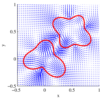
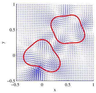
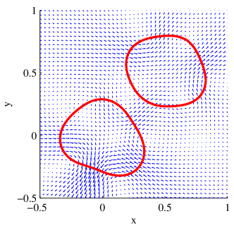
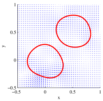
Figure 9: Interface in free space Stokes flow, driven by surface tension, at four times. The convective field $\mathbf{u}$ is obtained by evaluation the (singular) integrals in (25) on the interface. The flow fields shown are evaluations of (25) on a grid, used for visualization only.

The quadrature method described is trapezoidal, but with one interval of unequal length. In Figure 10 we establish second order convergence in $\infty$-norm away from the interface and second order convergence in $l_{1}$-norm on the interface, as the interface is refined. Here we have taken the interface circular, so that, by symmetry, the exact solution is $\mathbf{u}=0\,\,\forall\mathbf{x}_{0}$. Away from the interface we randomize a set of observation points, and on the interface we take as observation points the entire interface.

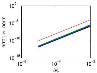
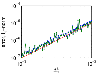
Figure 10: Convergence of boundary integral method (25), for $u$ and $v$, with second order given by solid line. Left: random sample set of observation points $\mathbf{x}_{0}$ away from the interface. Right: Observation points on the interface, i.e. singular integrands.

5 Incompressible Navier Stokes flow computations

We now demonstrate that our interface tracking method is applicable to the well established application of two-phase Navier-Stokes flow and that good results are obtained. There is not much here which is specific to our method. Indeed, this is an important point – our interface tracking method works well with established components in multi-phase flow computations.

5.1 Overview

The task of solving a multi-phase Navier-Stokes flow system is complicated for several reasons. At a basic level, solving the Navier-Stokes equations themselves is a challenging problem on its own. The incompressible Navier Stokes equations are given by

$$\rho\left(\frac{\partial\mathbf{u}}{\partial t}+(\mathbf{u}\cdot\nabla)\mathbf{u}\right)=-\nabla p+\mu\nabla^{2}\mathbf{u}+\mathbf{F}$$ (29)

$$\nabla\cdot\mathbf{u}=0$$ (30)

$$+(\text{Boundary conditions}).$$ (31)

where $\mu$ denotes viscosity and $\rho$ density. We will, for the remainder of this paper, consider the momentum equation in non-dimensional form:

$$\frac{\partial\mathbf{u}}{\partial t}+(\mathbf{u}\cdot\nabla)\mathbf{u}=-\nabla p+\frac{1}{\text{Re}}\nabla^{2}\mathbf{u}+\mathbf{F},$$ (32)

with $\text{Re}:=\frac{UL}{\mu}$, the Reynolds number.

The two main difficulties here are that the first (i.e. momentum) equation is non-linear, and that the space of admissible solutions is restricted (by the second equation) to be divergence free in the entire domain. We refer the reader to the excellent textbook by Acheson [36]. Several classes of numerical methods exist for Navier-Stokes, based on finite volume (FV), finite difference (FD) and finite element (FEM), as well as spectral methods. These often have high accuracy orders with respect to the spatial discretization. There are, however, much fewer methods that are fully second order accurate also in time. In the fluid mechanics community, this is generally regarded as of little consequence, since there are often physical time scales in the flow that are small. In this work we use a fairly basic pressure correction FD method, as presented in Section 5.2.

When a dynamic interface is added, e.g. the case of two immiscible liquids, the picture becomes more complicated still. The physical parameters of the flow may be different in the different fluids, and a two way coupling is introduced between the interface and the flow field. That is, the fluid acts upon the free surface which simultaneously acts upon the fluid. From a mathematical point of view it is clear that the equations of the two (or more) fluids and the dynamics of the free surface constitute one large, coupled and highly non-linear system. Furthermore, application specific challenges arise frequently. In the ubiquitous case of a bubble in a bulk fluid the most widely used formulation introduces a singular source term in the momentum equation (29) to mediate forces on the fluid from the interface, e.g. surface tension. The lack of regularity in the velocity and pressure solutions to the Navier Stokes equations presents significant numerical challenges. Here, we shall use the immersed boundary (IBM) and immersed interface (IIM) methods as presented in the following sections.

5.2 Numerical method for Navier Stokes

The numerical method to treat the Navier Stokes equations (29)-(31) is a finite difference method on a staggered (MAC) grid, which employs so called Chorin splitting. It is presented in detail in the textbook by Strang [37, Ch. 6.7], and a basic implementation due to Seibold is available on-line [38]. We summarize the time-discrete method here:

Compute a first intermediate velocity field, $\mathbf{u}^{*}$, by treating the non-linear term explicitly,

$$\frac{\mathbf{u}^{*}-\mathbf{u}^{n}}{\Delta t}=(\mathbf{u}^{n}\cdot\nabla)\mathbf{u}^{n}+\mathbf{F}.$$ (33)

To avoid a severe time-step restriction the diffusive term is treated implicitly and a second intermediate is obtained via

$$\frac{\mathbf{u}^{**}-\mathbf{u}^{*}}{\Delta t}=\frac{1}{\text{Re}}\Delta\mathbf{u}^{**}.$$ (34)

This, together with a discrete approximation for the spatial derivatives, constitute a linear system. Several appropriate solvers exist for this system depending on the memory constraints and the boundary conditions applied. The final result is obtained by applying a correction step,

$$\frac{\mathbf{u}^{n+1}-\mathbf{u}^{**}}{\Delta t}=-\nabla p^{n+1},$$ (35)

based on the pressure, which is obtained by solving a Poisson equation,

$$-\Delta p^{n+1}=-\frac{1}{\Delta t}\nabla\cdot\mathbf{u}^{**}.$$ (36)

We use central difference approximations for the spatial derivatives, so that $\nabla$ is replaced by the standard discrete nabla operator on a staggered grid $\nabla_{h}$. However, when applied to the convection step a moderate upwind bias is applied so as to not introduce a numerical instability (see [37, Ch. 6.7]).

Several remarks are in order. The pressure correction strategy is by no means the only one available for the task of decoupling the momentum equation from the incompressibility constraint. Another popular approach is the $\theta$-splitting method (see e.g. Glowinski and Pironneau [39]). A large body of work exist on the topic of pressure correction methods for Navier Stokes. The approach here dates back to Chorin [40] and may be seen as the most elementary method. Several more recent methods were presented and evaluated in a recent survey by Guermond et. al. [41]. The class of methods that Guermond refers to as consistent splitting methods can be seen to be more accurate than Chorin splitting. We also remind the reader that pressure correction methods do not necessarily have the property that both the non-divergence constraint and the prescribed boundary conditions are accurately satisfied simultaneously (due, at least in part, to the lack of a consistent numerical boundary condition for the pressure). Shedding light on these interesting topics is beyond the scope of this work, and we also content ourselves with using a first order accurate time discretization. A final remark concerns the efficiency of the method above: the linear solves in the diffusion and pressure correction steps involve constant system matrices. These matrices need only be factorized once, leaving just the back- and forward substitution steps to be performed in the time loop. The major constraint here is clearly the memory requirements of the factorized matrices, which may be significantly less sparse, but the efficiency obtained is of great practical value.

The flow solver couples to the interface tracking method previously presented, using Strang splitting (7).

5.3 Interface/flow coupling: immersed boundary formulation

As a basic case, let $\Gamma$ be a closed interface separating two liquids with equal density and viscosity. Two main approaches exist for coupling the motion of a dynamic interface with a incompressible, viscous bulk flow (described by the Navier Stokes equations above). First, separated grids may be generated for the separated flow regions – so called body fitted methods. The second class of methods follows the work of Peskin and collaborators [42, 43, 44, 45] on the immersed boundary (IB) method, where one views the separated flow regions as one system and a suitable force density is added to mediate the action of the interface on the fluid system. This method dates back to the 1970’s but still sees a remarkable amount of use. The 2002 survey paper by Peskin may be of particular interest to some readers [45].

Here, we shall use the IB formulation, with surface tension driving the flow internally. It is well known that the surface tension force as a function of Lagrangian variables on the interface can be formulated as

$$\mathbf{f}(s,t)=\sigma\kappa(s,t)\hat{n}(s,t),$$ (37)

where $\sigma\in\mathbb{R}^{+}$ is the surface tension coefficient, $\kappa$ is the interface curvature and $\hat{n}$ is the unit inward normal. Recall that the capillary number, Ca, is defined as $\text{Ca}:=\frac{U\mu}{\sigma}$. We may then write the non-dimensionalized force that will enter the momentum equation (32) in Eulerian variables as

$$\mathbf{F}(\mathbf{x},t) =\frac{1}{\text{Re}\,\text{Ca}}\int\kappa(s,t)\hat{n}(s,t)\delta_{\Gamma}\mathrm{d}s,$$ (38)

where $\delta_{\Gamma}$ is a Dirac measure on the interface, i.e. $\delta_{\Gamma}(\mathbf{x})=\delta(\mathbf{x}-\Gamma(s))$ and $\delta(\mathbf{x})$ is the composition of one-dimensional delta functions, $\delta(\mathbf{x})=\delta(x_{1})\delta(x_{2})$. Transformations from Lagrangian to Eulerian variables in this way are at the heart of the IB method and much related work. It is also appropriate to precisely define how the convective field in the interface advection ODE (1) arises:

$$\mathbf{u}(\Gamma,t):=\int_{\Omega}\mathbf{u}(\mathbf{x},t)\delta_{\Gamma}\mathrm{d}\mathbf{x}.$$ (39)

In order to complete the formulation of the discrete immersed boundary method one needs to introduce discrete delta function approximations. We refer the reader to a study by Tornberg and Engquist on the treatment of singular source terms [46]. We use the piecewise cubic delta function approximation introduced therein,

$$\delta_{2h}(x)=\begin{cases}\frac{1}{h}\phi(x/h),&\quad|x|\leq 2h\\ 0,&\quad|x|>2h\end{cases},$$ (40)

with

$$\phi(r)=\begin{cases}1-\frac{1}{2}|r|-|r|^{2}+\frac{1}{2}|r|^{3},&0\leq r\leq 1\\ 1-\frac{11}{6}|r|+|r|^{2}-\frac{1}{6}|r|^{3},&1<r\leq 2.\end{cases}$$ (41)

This delta function has narrow support on the grid and possesses a larger number of discrete moments than other commonly used variants. There are other good choices for the discrete delta function approximation. However, there is a generally held view, concerning stability, that the same approximation should be used in the “spreading” step (38) as in the evaluation step (39).

5.4 Immersed interface method

The singular source term introduced by the IBM gives rise to a jump discontinuity in the pressure, which is well understood physically: the pressure gradient balances the interfacial forces. This jump is

$$[p](s,t)=\mathbf{f}(s,t)\cdot\hat{n}(s,t).$$ (42)

That is, the pressure jump equals the magnitude of the interfacial force in the normal direction, which is simply $[p](s,t)=\sigma\kappa(s,t)$ in our case. Additional jump conditions need to be considered in settings where there are e.g. tangential stresses on the interface.

The immersed interface method (IIM), introduced and developed by LeVeque and collaborators in a series of papers [47, 48, 8], is in essence a evolution of the IBM where the jump conditions are corrected for in the numerical method rather than taken into the momentum equation as a source term. The textbook by Li and Ito [9], and a recent paper by Le et. al [10] may also be of interest. Derivations of the correction terms are given in the works cited above, and we humbly restate the relevant results here.

Going back to the NS method (33)-(36), drop the source term, $\mathbf{F}$ completely from the convective step, (33). The diffusive step (34) is unaltered, and the pressure correction step (35) and (36) we replace by

$$\left\{\begin{array}[]{l}\frac{\mathbf{u}^{n+1}-\mathbf{u}^{**}}{\Delta t}=-\nabla p^{n+1}+\mathbf{B}\\ -\Delta p^{n+1}=-\frac{1}{\Delta t}\nabla\cdot\mathbf{u}^{**}+C.\end{array}\right.$$ (43)

The correction terms, $\mathbf{B}=(B^{1},B^{2})$ and $C$, only have meaningful definitions as discrete functions. Recall that we are working on a staggered (MAC) grid. It turns out to be natural to evaluate the correction term $B^{1}$ at intersections with horizontal grid lines, so that $B^{1}_{i-1/2,j}=[p]/\Delta x$ if the interface cuts the grid between points $(i,j)$ and $(i-1,j)$, and zero otherwise. Correspondingly, the correction on the $y$-grid is given by $B^{2}_{i,j-1/2}=[p]/\Delta y$ if the interface cuts the vertical grid lines between $(i,j)$ and $(i,j-1)$, and zero otherwise. Finally,

$$B^{1}_{ij}=\frac{1}{2}\left(B^{1}_{i-1/2,j}+B^{1}_{i+1/2,j}\right),$$ (44)

$$B^{2}_{ij}=\frac{1}{2}\left(B^{1}_{i,j-1/2}+B^{1}_{i,j+1/2}\right),$$ (45)

$$C_{ij}=(\nabla_{h}\cdot\mathbf{B})_{ij}.$$ (46)

This concludes the formulation of the discrete immersed interface method.

5.4.1 IBM vs. IIM: Accuracy

Due to the smearing of the interface introduced by the regularized delta function, the IBM will at most attain first order accuracy for problems with non-smooth solutions. The IIM has been shown to produce second order accurate results.

5.4.2 IBM vs. IIM: Stability

Interestingly, there has been much recent work on the stability of the IBM, despite the many years since it was introduced. Peskin himself emphasizes stability as one of the outstanding challenges for the IBM in his Acta Numerica paper [45]. Newren et. al. [49] appear to have resolved this issue by providing a general stability theory for the IBM applied to Stokes flow. They show unconditional stability for a Crank-Nicholson method and backward Euler method. Following that paper, Newren et. al. [50] discuss practical solver strategies for semi- and fully implicit immersed boundary methods for Navier Stokes. They substantiate the widely held view that fully explicit methods are competitive, despite the short time steps, due to the high computational costs associated with the iterative methods needed in implicit IBM formulations. In another recent paper, Hou and Shi [51] also obtain unconditionally stable discretizations for the Stokes case. Based on earlier work by Hou, Lowengrub and Shelley [52] and their unconditionally stable method, they go to great lengths to derive an efficient semi-implicit method with good stability properties. While this appears to be the most efficient method known at present, it relies heavily on spectral properties of the spatial discretization and, hence, is only applicable in certain cases.

Newren et. al. point out two conditions as sufficient to prove stability of immersed boundary methods: First, the spreading and interpolation must be adjoint operators. Second, the velocity field needs to be discretely divergence free. Hou and Shi reiterate this conclusion. Hou and Shi also make a separate point about the need to alleviate the stiffness in the interface/flow coupling, and go about it by using the arc-length and tangent angle formulation (cf. [52, 51]).

Little is known to date about the stability properties of immersed interface methods. There are several vague comments on stability in the IIM literature [48, 8, 10, 9]. The authors seem to agree that the explicit methods suffer from a severe stiffness, which motivates implicit methods. Going back to the sufficient conditions for stability of IB methods, it is clear that there is no adjointness property applicable in the IIM case (since there is no spreading operator). However, one could reasonably expect the non-divergence condition to be better handled by the IIM: In the IBM, as the pressure jump gets bigger the smeared pressure becomes under-resolved numerically and oscillatory near the interface. This would lead to a less accurate pressure correction, and hence a failure to be accurately divergence free in the velocity. The pressure solve is more accurate in the IIM. Further, the idea of formulating the interface problem in terms of arc-length and tangent angle has not been applied to the IIM as far as we know.

5.5 Numerical results: Navier-Stokes

5.5.1 Shear flow

We illustrate the NS/IBM solver by considering a drop in shear flow. The shear velocity is imposed as a Dirichlet boundary condition on the top and bottom boundaries, ramped up via

$$u(1,t)=\begin{cases}\frac{u_{\infty}}{2}\left(1-\cos\left(\frac{\pi t}{t_{\infty}}\right)\right),&t\leq t_{\infty}\\ u_{\infty}&t>t_{\infty}\end{cases}$$

for some ramp-up time $t_{\infty}$ and shear velocity $u_{\infty}$. We let $u(0,t)=-u(1,t)$. In the $x$-direction we impose periodic boundary conditions. In Figure 11 we present computational results with different coefficients of surface tension. Here we used $u_{\infty}=1$, $t_{\infty}=1/5$ and 80 grid-points in the $y$-direction. These results could equally well have been obtained with the immersed interface method given above. Throughout this section we use the channel height, $L_{y}=1$, when determining the Reynolds number.

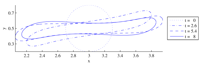
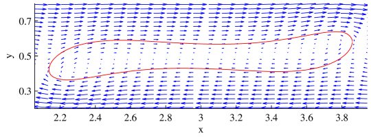
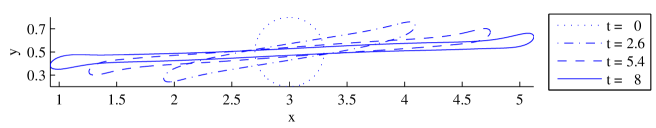
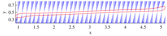
Figure 11: Interface location at various times, and flow field at $t=8$. Top pair: $\text{Re}=1,\text{Ca}=1$. Below critical Ca, the interface reaches a steady state. Bottom pair: $\text{Re}=1,\text{Ca}=2$. Above critical Ca, no steady interface is obtained.

5.5.2 Convergence

The method used here is not more than first order accurate, as discussed prior. To verify this we ran numerical convergence tests using a shear flow setup. Here we use an initially circular drop with radius $r=1/3$ centered in a unit square domain. The shear boundary conditions are ramped up as above, with $t_{\infty}=1/5$ and we compute until $t=1/4$. With $\text{Re}=\text{Ca}=1$ we get, at that time, that the interface is moderately deformed, but not close to a steady state.

In Tables 1 and 2 we give convergence results for the immersed boundary and immersed interface methods respectively, as the grid is refined. The ratio $h/\Delta t$ is kept fixed, so several hundred time steps are taken on the finest mesh. These results indicate the expected overall first order convergence for both methods.

Here we let $u_{i}$ be a sequence of computed solutions, and assume the error with respect to some unknown exact solution $\tilde{u}$ behaves like $\|u_{i}-\tilde{u}\|\approx O(h_{i}^{p})+O(\Delta t^{p})$. We define $\Delta^{i}:=\|u_{i}-u_{i-1}\|$ for various norms and have estimates of the convergence order $p=\log_{2}(\Delta^{i+1}/\Delta^{i})$ as the grid is refined by a factor 2. To see a benefit in terms of accuracy from using the immersed interface method, a second order accurate time stepping method for the flow solver would have to be implemented.

$N$	$\Delta_{u}$	$p_{u}$	$\Delta_{v}$	$p_{v}$
44
88	0.011282		0.000421
176	0.005611	1.007641	0.000202	1.056737
352	0.002873	0.965510	0.000098	1.042040

$N$	$\Delta_{u}$	$p_{u}$	$\Delta_{v}$	$p_{v}$
44
88	0.011329		0.000540
176	0.005636	1.007214	0.000255	1.082531
352	0.002881	0.968202	0.000124	1.039785

$N$	$\Delta_{u}$	$p_{u}$	$\Delta_{v}$	$p_{v}$
44
88	0.013639		0.002467
176	0.006866	0.990110	0.001237	0.995364
352	0.003483	0.979443	0.000658	0.912272

Table 1: NS/IBM grid refinement study, shear flow, Top: $l_{1}$, Middle: $l_{2}$, Bottom: $l_{\infty}$. See Section 5.5.2

$N$	$\Delta_{u}$	$p_{u}$	$\Delta_{v}$	$p_{v}$
44
88	0.011935		0.000493
176	0.005223	1.192320	0.000282	0.807506
352	0.002829	0.884727	0.000107	1.391809

$N$	$\Delta_{u}$	$p_{u}$	$\Delta_{v}$	$p_{v}$
44
88	0.011969		0.000645
176	0.005274	1.182247	0.000378	0.768790
352	0.002841	0.892364	0.000144	1.391774

$N$	$\Delta_{u}$	$p_{u}$	$\Delta_{v}$	$p_{v}$
44
88	0.015243		0.004002
176	0.008466	0.848441	0.001872	1.096254
352	0.004081	1.052766	0.000742	1.335409

Table 2: NS/IIM grid refinement study, shear flow, Top: $l_{1}$, Middle: $l_{2}$, Bottom: $l_{\infty}$. See Section 5.5.2

5.5.3 Brief comparative study

Whereas a full comparison between the immersed interface- and boundary method including solution methods would be valuable, it is beyond the scope of this work. The space of parameters, e.g. discretization and solution methods, capillary- and Reynolds numbers, is very large. Still, we think some brief comparisons are in order.

First, for the simple shear flow setup described above we compare the results obtained with the immersed interface- and boundary methods with explicit time stepping. As can be seen in Figure 12, there is a small but visible discrepancy. Here, the domain was $[0\,\,2]\times[0\,\,1]$, with a grid with $h_{x}=h_{y}=1/100$ and the interface was discretized with $\Delta\xi=1/200$. Again, the physical parameters were $\text{Re}=\text{Ca}=1$. In this test we noted that the IIM was more prone to going unstable, as expected. We had to take $\Delta t=1/300$ with the IBM and $\Delta t=1/3000$ with the IIM, to get stable computations.

For a more challenging case, e.g. with Ca several orders below unity, we expect to see the implicit (CN) method stable for larger time steps than the explicit method. However, this has not been evident to us – at least not to the extent that the overall computational cost of a run becomes smaller with an implicit method. That implicit methods fail to be competitive for the IBM is in line with results by Newren et. al. [50] and others. We have to conclude with noting that more research is need to illuminate the efficient deployment of immersed boundary- and interface methods.

In Figure 13 we consider a shear flow case where the Reynolds number goes to zero, i.e. the limit of Stokes flow. Here we compare the results from the Navier-Stokes (IBM) method with the boundary integral Stokes method (Section 4) and find excellent agreement as $\text{Re}\rightarrow 0$.

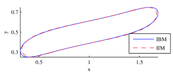
Figure 12: Interface in shear flow, at time $T=2$, with both IIM and IBM.

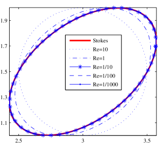
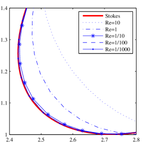
Figure 13: Interface in shear flow, at time $T=1$, and $\text{Ca}=5$. We illustrate that as $\text{Re}\rightarrow 0$, the Navier-Stokes (IBM) method converges to the results from the boundary integral Stokes method (cf. Section 4). Here the interface is initially circular, with diameter 1, and at location $(3,3/2)$, in a domain $[0,6]\times[0,3]$ and shear boundary conditions discussed in Section 5.5.1. Note that the $T=1$ is before a steady state is reached. Bottom: close-up from above.

6 Conclusions and outlook

We have introduced an interface tracking method which is both Eulerian and explicit, as motivated by current and future needs for micro- and complex flow modeling and simulation. For instance, the PDE-based methods by Khatri and Tornberg [6] for simulating soluble and insoluble surfactants fit naturally into this framework.

The method presented is based on a domain decomposition approach, where the interface is split into segments, or patches. On each patch a hyperbolic PDE is solved in time to update the interface location, and adjacent segments are coupled via an exchange of ghost points. One explicit and one implicit time step method was presented, both second order accurate.

Numerically, the accuracy and consistency order of the proposed method was established: second order in $\infty$-norm for the interface location. We were also able to present first and second order convergence in the interface curvature – a quantity which is known to be hard to compute (without filtering). Mass conservation was found to be well behaved, converging at second order with a constant several orders of magnitude below unity.

An extension of the method was also presented, which made use of a decomposition of the velocity field into translation and rotation components, as motivated by a variety of flow applications where such components tend to dominate. The resulting method was also shown numerically to have the desirable accuracy characteristics mentioned above.

We treated two applications: Stokes and Navier-Stokes flow. The first used a boundary integral method, and illustrated how an application with integration over the interface can be treated in our framework. We found that it was simple to derive and analyze a method which was second order accurate for integrals of the Greens’ function for Stokes flow in free space.

Finally, with the application of our method to two-phase incompressible Navier Stokes flow, we showed that our method works well with existing components for such problems. Both the immersed interface- and immersed boundary method was used. We gave and evaluated a first order accurate method for solving the Navier-Stokes equations and presented computations of a bubble in shear flow. The two-phase flow results are by no means new, but serve to underline that our method can be used in established applications with good results.

However, as of yet, we have not generalized our method to 3D in sufficient generality. The framework and equations generalize naturally – the difficulty is representing closed surfaces as a union of patches, in a way that allows the patches to couple together robustly. One would like to use regular grids in 2D for these patches, to be able to use well-established numerical method for advecting the interface, computing curvature and quadrature etc.

None the less, we believe that at a method that is explicit in the interface location and Eulerian is very useful for treating complex interface tracking applications. There is a wealth of interesting flow applications on the micro scale where continuum modeling on the interface becomes relevant.

References

References

- [1] S. Osher, J. A. Sethian, Fronts propagating with curvature-dependent speed - algorithms based on hamilton-jacobi formulations, J. Comp. Phys 79 (1988) 12–49.
- [2] D. Adalsteinsson, J. A. Sethian, A fast level set method for propagating interfaces, J. Comp. Phys 118 (1995) 269–277.
- [3] J. Sethian, Fast marching methods, SIAM Rev. 41 (1999) 199–235.
- [4] M. Sussman, P. Smereka, S. Osher, A level set approach for computing solutions to incompressible 2-phase flow, J. Comp. Phys 114 (1994) 146–159.
- [5] E. Olsson, G. Kreiss, A conservative level set method for two phase flow, J. Comp. Phys 210 (2005) 225–246.
- [6] S. M. Khatri, A numerical method for two phase flows with insoluble and soluble surfactants, Ph.D. thesis, Courant Institute of Mathematical Sciences, New York University (2009).
- [7] S. Khatri, A.-K. Tornberg, A numerical method for two phase flows with insoluble surfactants, Comput. Fluids 49 (2011) 150–165.
- [8] L. Lee, R. Leveque, An immersed interface method for incompressible navier-stokes equations, SIAM J. Sci. Comput. 25 (2003) 832–856. doi:10.1137/S1064827502414060.
- [9] Z. Li, K. Ito, The Immersed Interface Method, SIAM, Philadelphia, 2006.
- [10] D. V. Le, B. C. Khoo, J. Peraire, An immersed interface method for viscous incompressible flows involving rigid and flexible boundaries, J. Comp. Phys 220 (2006) 109–138. doi:10.1016/j.jcp.2006.05.004.
- [11] J. A. Warren, W. J. Boettinger, Prediction of dendritic growth and microsegregation patterns in a binary alloy using the phase-field method, Acta Metallurgica et Materialia 43 (1995) 689–703.
- [12] A. Karma, W. J. Rappel, Phase-field method for computationally efficient modeling of solidification with arbitrary interface kinetics, Phys. Rev. E 53 (1996) R3017–R3020.
- [13] C. W. Hirt, B. D. Nichols, Volume of fluid (VOF) method for the dynamics of free boundaries, J. Comp. Phys 39 (1981) 201–225.
- [14] E. Puckett, A. Almgren, J. Bell, D. Marcus, W. Rider, A high-order projection method for tracking fluid interfaces in variable density incompressible flows, J. Comp. Phys 130 (1997) 269–282.
- [15] S. O. Unverdi, G. Tryggvason, A front-tracking method for viscous, incompressible, multi-fluid flows, J. Comp. Phys 100 (1992) 25–37.
- [16] G. Tryggvason, B. Bunner, A. Esmaeeli, D. Juric, N. Al-Rawahi, W. Tauber, J. Han, S. Nas, Y. Jan, A front-tracking method for the computations of multiphase flow, J. Comp. Phys 169 (2001) 708–759. doi:10.1006/jcph.2001.6726.
- [17] J. Glimm, J. Grove, X. Li, K. Shyue, Y. Zeng, Q. Zhang, Three-dimensional front tracking, SIAM J. Sci. Comput. 19 (1998) 703–727.
- [18] D. Enright, R. Fedkiw, J. Ferziger, I. Mitchell, A hybrid particle level set method for improved interface capturing, J. Comp. Phys 183 (2002) 83–116.
- [19] D. Gaudlitz, N. A. Adams, On improving mass-conservation properties of the hybrid particle-level-set method, Comput. Fluids 37 (2008) 1320–1331. doi:10.1016/j.compfluid.2007.11.005.
- [20] Z. Wang, J. Yang, B. Koo, F. Stern, A coupled level set and volume-of-fluid method for sharp interface simulation of plunging breaking waves, Int. J. Multiphase Flow 35 (2009) 227–246. doi:10.1016/j.ijmultiphaseflow.2008.11.004.
- [21] J. W. Demmel, Applied Numerical Linear Algebra, SIAM, 1997.
- [22] A. Toselli, O. Widlund, Domain Decomposition Methods, Springer, 2004.
- [23] M. Nakahara, Geometry, Topology and Physics, Second Edition, 2nd Edition, Taylor & Francis, 2003.
- [24] A. Tornberg, B. Engquist, The segment projection method for interface tracking, Commun. Pure Appl. Math. 56 (2003) 47–79.
- [25] B. Engquist, O. Runborg, A. Tornberg, High-frequency wave propagation by the segment projection method, J. Comp. Phys 178 (2002) 373–390. doi:10.1006/jcph.2002.7033.
- [26] R. J. LeVeque, Finite Volume Methods for Hyperbolic Problems, Cambridge University Press, 2002.
- [27] C. Tu, C. S. Peskin, Stability and instability in the computation of flows with moving immersed boundaries - a comparison of 3 methods, SIAM J. Sci. Stat. Comp. 13 (1992) 1361–1376.
- [28] T. Pavlidis, S. L. Horowitz, Segmentation of plane curves, IEEE Trans Comput 23 (8) (1974) 860–870. doi:http://dx.doi.org/10.1109/T-C.1974.224041.
- [29] J. A. Ventura, J.-M. Chen, Segmentation of two-dimensional curve contours, Pattern Recogn 25 (10) (1992) 1129 – 1140. doi:DOI: 10.1016/0031-3203(92)90016-C.
- [30] N. Katzir, M. Lindenbaum, M. Porat, Curve segmentation under partial occlusion, IEEE Trans Pattern Anal 16 (1994) 513–519.
- [31] A. Kolesnikov, P. Franti, Polygonal approximation of closed discrete curves, Pattern Recogn 40 (2007) 1282–1293.
- [32] C. Pozrikidis, Boundary Integral and Singularity Methods for Linearized Viscous Flow, Cambridge University Press, 1992.
- [33] S. Kim, S. J. Karrila, Microhydrodynamics: Principles and Selected Applications, Butterworth-Heinemann, 1991.
- [34] C. Pozrikidis, Interfacial dynamics for Stokes flow, J. Comp. Phys 169 (2001) 250–301. doi:10.1006/jcph.2000.6582.
- [35] C. Pozrikidis, The instability of a moving viscous drop, J. Fluid Mech. 210 (1990) 1–21.
- [36] D. J. Acheson, Elementary Fluid Dynamics, Oxford University Press, 1990.
- [37] G. Strang, Computational Science and Engineering, Wellesley-Cambridge Press, 2007.
- [38] B. Seibold, http://www-math.mit.edu/cse/codes/mit18086_navierstokes.m, Retreived Feb. 2009 (2007).
- [39] R. Glowinski, O. Pironneau, Finite elements methods for Navier-Stokes equations, Annu. Rev. Fluid Mech. vol.24 (1992) 167–204.
- [40] A. J. Chorin, Numerical solution of the navier-stokes equations, Math. Comput. 22 (1968) 745–762.
- [41] J. L. Guermond, P. Minev, J. Shen, An overview of projection methods for incompressible flows, Comput. Meth. Appl. Mech. Eng. 195 (2006) 6011–6045. doi:10.1016/j.cma.2005.10.010.
- [42] C. S. Peskin, Numerical-analysis of blood-flow in heart, J. Comp. Phys 25 (3) (1977) 220–252.
- [43] C. S. Peskin, D. M. McQueen, Modeling prosthetic heart-valves for numerical-analysis of blood-flow in the heart, J. Comp. Phys 37 (1) (1980) 113–132.
- [44] C. S. Peskin, B. F. Printz, Improved volume conservation in the computation of flows with immersed elastic boundaries, J. Comp. Phys 105 (1) (1993) 33–46.
- [45] C. S. Peskin, The immersed boundary method, Acta Numerica 11 (2002) 479–517.
- [46] A. Tornberg, B. Engquist, Numerical approximations of singular source terms in differential equations, J. Comp. Phys 200 (2004) 462–488. doi:10.1016/j.jcp.2004.04.011.
- [47] R. LeVeque, Z. Li, The immersed interface method for elliptic-equations with discontinuous coefficients and singular sources, SIAM J. Numer. Anal. 31 (4) (1994) 1019–1044.
- [48] R. LeVeque, Z. Li, Immersed interface methods for Stokes flow with elastic boundaries or surface tension, SIAM J. Sci. Comput. 18 (3) (1997) 709–735.
- [49] E. P. Newren, A. L. Fogelson, R. D. Guy, R. M. Kirby, Unconditionally stable discretizations of the immersed boundary equations, J. Comp. Phys 222 (2) (2007) 702–719. doi:10.1016/j.jcp.2006.08.004.
- [50] E. P. Newren, A. L. Fogelson, R. D. Guy, R. M. Kirby, A comparison of implicit solvers for the immersed boundary equations, Comput. Meth. Appl. Mech. Eng. 197 (2008) 2290–2304. doi:10.1016/j.cma.2007.11.030.
- [51] T. Y. Hou, Z. Shi, Removing the stiffness of elastic force from the immersed boundary method for the 2D Stokes equations, J. Comp. Phys 227 (21, Sp. Iss. SI) (2008) 9138–9169. doi:10.1016/j.jcp.2008.03.002.
- [52] T. Y. Hou, J. S. Lowengrub, M. J. Shelley, Removing the stiffness from interfacial flow with surface-tension, J. Comp. Phys 114 (1994) 312–338.