Variational Monte Carlo approach to the two-dimensional Kondo lattice model

Abstract

We study the phase diagram of the Kondo-lattice model with nearest-neighbor hopping in the square lattice by means of the variational Monte Carlo technique. Specifically, we analyze a wide class of variational wave functions that allow magnetic and superconducting order parameters, so to assess the possibility that superconductivity might emerge close to the magnetic instability, as often observed in heavy fermion systems. Indeed, we do find evidence of $d$-wave superconductivity in the paramagnetic sector, i.e., when magnetic order is not allowed in the variational wave function. However, when magnetism is allowed, it completely covers the superconducting region, which thus disappears from the phase diagram.

I Introduction

The Kondo lattice model (KLM) describes localized magnetic moments that interact with a single band of itinerant electrons via an antiferromagnetic exchange coupling $J$. This model has been introduced long ago by Doniach, doniach and, since then, has been widely invoked to describe the physics of heavy-fermion materials. stewart Three ingredients define the KLM: the bandwidth $W$ of the conduction electrons (usually denoted by $c$ electrons), their density $n_{c}$, and the Kondo exchange $J$ that controls the coupling between the local moments and the spin density of $c$-electrons. The localized moments (denoted by $f$ electrons) are anchored to the sites of a regular lattice. The phase diagram of the KLM depends in a non-trivial way on $J/W$ and the electron density $n_{c}$. In one spatial dimension, the KLM has been intensively studied and shows three distinct phases. tsunetsugu In the compensated case, one conduction electron per localized spin, i.e., $n_{c}=1$, it is a so-called Kondo insulator with a charge as well as a spin gap without any magnetic order, a kind of spin-liquid insulator. For $n_{c}\not=1$, it is either a paramagnetic metal for low $J/W$, or a ferromagnetic metal for larger $J/W$. In higher dimensions, where the $SU(2)$ spin symmetry can be spontaneously broken, the phase diagram is expected to enrich and display a critical point separating a paramagnetic heavy-fermion metal from a different metallic phase with long-range magnetic order. doniach ; lacroix Indeed, in analogy with the Kondo effect that occurs in the case of a single magnetic impurity, the conduction electrons may screen the localized moments, thus forming a global singlet state. However, such a Kondo screening is thwarted by the tendency to magnetic ordering of the localized moments. In fact, the latter ones interact mutually via the Ruderman-Kittel-Kasuya-Yosida (RKKY) mechanism, through an effective exchange $J_{eff}(q)\propto-J^{2}\,\Re e\chi(q,\omega=0)$ mediated by the magnetic polarization $\chi(q,\omega)$ of the conduction band. The competition between Kondo screening (that favors a paramagnetic ground state) and RKKY interaction (that favors magnetically ordered states) is the heart of a frustrating behavior, which may lead to genuine quantum phase transitions.doniach Furthermore, other physical processes may profit from the balanced competition between Kondo screening and magnetic ordering nearby the transition, and make novel phases to intrude, most notably superconductivity. Indeed, the discovery of superconductivity in CeCu₂Si₂, steglich and subsequently in several other heavy-fermion materials, unveiled the rich variety of phenomena of these strongly-correlated systems. It is widely believed that, in heavy-fermion compounds, superconductivity is not the conventional phonon-mediated one, but most likely it is caused by antiferromagnetic spin fluctuations. mathur

Recent experiments of the Hall coefficient in the heavy-fermion material YbRh₂Si₂, pashen have provided new intriguing elements that renewed interest in the phase diagram of the KLM. In particular, the rapid jump of the Hall coefficient pashen ; schoeder ; gegenwart ; custers ; coleman ; friedmann ; custers2 is suggestive of a sudden change of the Fermi surface topology at, or close to, the quantum phase transition between the non-magnetic metal and the magnetic one. In the conventional view of heavy-fermions, the localized spins are promoted in the conduction band through the Kondo effect. A mass-enhanced Fermi liquid is thus settled down, with a “large” Fermi surface that includes the conduction as well as the localized electrons. In the simplest scenario of a spin-density-wave quantum phase transition, hertz ; millis magnetic ordering is indeed expected to modify the topology of the Fermi surface by appearance of the magnetic Bragg reflections. In addition, the Fermi surface reconstruction across the magnetic field induced transition in YbRh₂Si₂ can also be simply interpreted as a Zeeman driven Lifshitz transition of the heavy quasiparticles. vojta However, an alternative scenario is possible in which the Kondo effect dies out at the transition point, si hence the local moments suddenly stop contributing to the volume of the Fermi surface, which then counts only the number of $c$ electrons. In the language of the Anderson lattice model, which maps for strong repulsion onto the KLM, the death of the Kondo effect would translate into the Mott localization of the $f$ electrons, whose magnetic ordering would then be only a by-product rather then the driving source. Indeed, there are suggestions that the Kondo-breakdown and the onset of magnetic order in the Anderson lattice model are distinct phenomena, which may occur at different points of the phase diagram. senthil ; deleo This scenario has been indirectly supported by variational Monte Carlo calculations ogata and by the Gutzwiller approximation lanata in the KLM on a square lattice. Indeed, these works found evidence of two distinct phase transitions, one given by the continuous appearance of long-range magnetic order and another one related to an abrupt topological change of the Fermi surface. The same outcome of two distinct transitions has been later observed also within the dynamical cluster approximation (DCA). assaad In spite of all efforts, such an interesting issue like remains open.

In this paper, we investigate the KLM in two dimensions paying attention not only to magnetism, but also to the possible emergence of superconductivity in its proximity. We use both mean-field and variational Monte Carlo approaches. As far as the former one is concerned, an analytical treatment of the long-range antiferromagnetic phase is possible only at compensation, $n_{c}=1$, where calculations have been already performed. zhang Here, we go beyond the results of Ref. zhang, and consider also the uncompensated regime, $n_{c}<1$, by solving numerically the Hartree-Fock equations. Furthermore, we generalize the previous calculations based upon the variational Monte Carlo approach ogata or the Gutzwiller approximation lanata and introduce additional correlations inside the trial wave function, among which superconducting ones. In particular, our variational calculations show that superconductivity is indeed stabilized in the paramagnetic sector in a region of the phase diagram close to $n_{c}=1$ and not too large $J/W$. However, when magnetism is allowed in the variational wave function, an antiferromagnetic phase emerges and completely covers the superconducting dome. Therefore, at least within the variational approach and in our model where the only source of magnetic frustration is deviation from the compensated regime, we do not find any superconducting region at the border between antiferromagnetic and heavy-fermion metal.

The paper is organized as follow: in section II, we introduce the microscopic model and discuss the methods that we use; in section III, we present our numerical results for both mean-field and variational approximations; and, finally, in section IV, we draw our conclusions.

II Model and methods

The KLM model on the two-dimensional square lattice is defined by:

$${\cal H}=-t\sum_{\langle i,j\rangle,\sigma}c^{\dagger}_{i,\sigma}c^{\phantom{\dagger}}_{j,\sigma}+h.c.+J\sum_{i}{\bf S}_{i}\cdot{\bf s}_{i}$$ (1)

where $\langle i,j\rangle$ denotes nearest-neighbor sites $i$ and $j$ and $c^{\dagger}_{i,\sigma}$ ($c^{\phantom{\dagger}}_{i,\sigma}$) creates (destroys) an itinerant electron at site $i$ with spin $\sigma$; ${\bf s}_{i}=(s^{x}_{i},s^{y}_{i},s^{z}_{i})$ is the spin operator for the $c$-electrons, i.e., $s^{\alpha}_{i}=1/2\sum_{\sigma,\sigma^{\prime}}c^{\dagger}_{i,\sigma}\tau^{\alpha}_{\sigma,\sigma^{\prime}}c^{\phantom{\dagger}}_{i,\sigma^{\prime}}$, $\tau^{\alpha}$ being the Pauli matrices. Similarly, ${\bf S}_{i}=(S^{x}_{i},S^{y}_{i},S^{z}_{i})$ is the spin operator for the localized $f$ electrons, $S^{\alpha}_{i}=1/2\sum_{\sigma,\sigma^{\prime}}f^{\dagger}_{i,\sigma}\tau^{\alpha}_{\sigma,\sigma^{\prime}}f^{\phantom{\dagger}}_{i,\sigma^{\prime}}$. By constraint there is one $f$ electron per each site. The exchange coupling is antiferromagnetic, i.e., $J>0$, and we shall take all energies measured in units of $t$.

II.1 Mean-field approach

The simplest approach to the KLM of Eq. (1) is the mean-field approximation, in which the spin-spin interaction is decoupled to bring about a non-interacting Hamiltonian. We shall implement Hartree-Fock by assuming finite the following average values, to be determined self-consistently:

$$V = \langle c^{\dagger}_{i,\sigma}f^{\phantom{\dagger}}_{i,\sigma}\rangle=\langle f^{\dagger}_{i,\sigma}c^{\phantom{\dagger}}_{i,\sigma}\rangle,$$ (2)

$$m_{c} = -(-1)^{R_{i}}\,\langle s^{z}_{i}\rangle,$$ (3)

$$m_{f} = (-1)^{R_{i}}\,\langle S^{z}_{i}\rangle.$$ (4)

$V$ denotes the (site-independent) $c{-}f$ hybridization, responsible in mean-field for the creation of the Kondo singlet; $m_{c}$ and $m_{f}$ are the staggered magnetizations of conduction and localized electrons, respectively, which have opposite sign because of the antiferromagnetic exchange $J$. In addition, a Lagrange multiplier $\mu_{f}$ must be included to enforce (on average) the $f$-orbital occupancy, i.e., $n_{f}=1$.

In momentum space, the antiferromagnetic mean-field Hamiltonian can be cast in a $4\times 4$ matrix form:

$$\begin{split}{\cal H}_{\rm AF}=\sum\limits_{k\in MBZ,\sigma}\left[\begin{array}[]{cccc}c^{\dagger}_{k,\sigma}&c^{\dagger}_{k+Q,\sigma}&f^{\dagger}_{k,\sigma}&f^{\dagger}_{k+Q,\sigma}\end{array}\right]\times\\ \begin{bmatrix}\epsilon_{k}&\frac{1}{2}Jm_{f}\sigma&-\frac{3}{4}JV&0\\ \frac{1}{2}Jm_{f}\sigma&-\epsilon_{k}&0&-\frac{3}{4}JV\\ -\frac{3}{4}JV&0&-\mu_{f}&-\frac{1}{2}Jm_{c}\sigma\\ 0&-\frac{3}{4}JV&-\frac{1}{2}Jm_{c}\sigma&-\mu_{f}\end{bmatrix}\left[\begin{array}[]{c}c^{\phantom{\dagger}}_{k,\sigma}\\ c^{\phantom{\dagger}}_{k+Q,\sigma}\\ f^{\phantom{\dagger}}_{k,\sigma}\\ f^{\phantom{\dagger}}_{k+Q,\sigma}\end{array}\right],\end{split}$$ (5)

where the sum over $k$ is restricted to the reduced (magnetic) Brillouin zone. In order to compute the total energy, the constant term $(3JV^{2}/2+Jm_{c}m_{f}+\mu_{f})N$ must be added ($N$ being the number of sites).

The paramagnetic state is found by imposing $m_{c}=m_{f}=0$ and corresponds to the $2\times 2$ matrix Hamiltonian:

$${\cal H}_{\rm PM}=\sum\limits_{k,\sigma}\left[\begin{array}[]{cc}c^{\dagger}_{k,\sigma}&f^{\dagger}_{k,\sigma}\end{array}\right]\begin{bmatrix}\epsilon_{k}&V\\ V&-\mu_{f}\end{bmatrix}\left[\begin{array}[]{c}c^{\phantom{\dagger}}_{k,\sigma}\\ f^{\phantom{\dagger}}_{k,\sigma}\end{array}\right].$$ (6)

The self-consistency conditions Eqs. (2), (3), and (4) are solved numerically on finite size systems with $N$ sites, number that we scale to get reliable estimates in the thermodynamic limit. We mention that an analytic solution of the problem is possible only in the compensated regime, while in general numerical calculations are needed. In practice, we numerically diagonalize the $4\times 4$ matrix for all $k$ points independently and then fill the bands with the lowest orbitals; the mean-field parameters are numerically calculated and the procedure is iterated until convergence is reached. At the mean-field level, a superconducting singlet order parameter $\sum_{\sigma}\,\sigma\,\langle c^{\dagger}_{k,\sigma}f^{\dagger}_{k,-\sigma}\rangle$ is not independent from the hybridization, because of the charge-isospin $SU(2)$ symmetry displayed by the $f$ electrons.

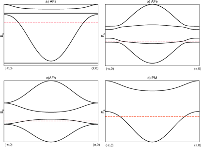
Figure 1: (Color on-line) Quasi-particle band structure for various phases: the AFs (a) has flat $f$ bands, due to the full decoupling between $f$ and $c$ electrons and a small Fermi surface; the antiferromagnetic phases with electron-like and hole-like Fermi surfaces are denoted by AFe (b) and AFh (c), respectively; finally, PM (d) is a paramagnetic (metallic) phase. The dashed red line indicates the chemical potential.

Within the AF state, we find three different cases, depending on the magnitude of variational parameters. In the following, we will adopt the notations of Ref. ogata, . Whenever the hybridization parameter vanishes, i.e., $V=0$, the localized electrons decouple from the conducting ones and they do not contribute to the volume enclosed by the Fermi surface, in this case we have an antiferromagnetic state with a “small” Fermi surface (denoted by AFs). By adding a small hybridization to the AFs, we end up with a state which has an electron-like Fermi surface, the so-called AFe. Finally, in the case where the hybridization $V$ is large and the magnetic order parameter small, we have a hole-like Fermi surface, the so-called AFh. Here, the $f$ electrons participate to the total volume enclosed by the Fermi surface, which is therefore “large”. A qualitative picture of all these cases, together with the simple paramagnetic state is depicted in Fig. 1.

II.2 Variational wave functions

In order to go beyond the mean-field approximation, we consider correlated variational wave functions, in which the constraint of one $f$ electron per site is imposed exactly via a Gutzwiller projector. This is achieved through the projected variational wave function:

$$|\Psi\rangle={\cal P}_{f}|\Psi_{\rm MF}\rangle,$$ (7)

where ${\cal P}_{f}$ is the projector which enforces single occupation of $f$ orbitals on each site. Here, $|\Psi_{MF}\rangle$ is an uncorrelated wave function defined as the ground state of a non-interacting variational Hamiltonian ${\cal H}_{\rm MF}$ that may contain, in addition to the mean-field parameters of the previous section II.1, also direct $f{-}f$ hopping as well as superconducting terms:

$$\chi_{i,j}^{ff} = \langle f^{\dagger}_{i,\sigma}f^{\phantom{\dagger}}_{j,\sigma}\rangle,$$ (8)

$$\Delta_{i,j}^{ff} = \langle f^{\dagger}_{i,\uparrow}f^{\dagger}_{j,\downarrow}+f^{\dagger}_{j,\uparrow}f^{\dagger}_{i,\downarrow}\rangle,$$ (9)

$$\Delta_{i,j}^{cc} = \langle c^{\dagger}_{i,\uparrow}c^{\dagger}_{j,\downarrow}+c^{\dagger}_{j,\uparrow}c^{\dagger}_{i,\downarrow}\rangle,$$ (10)

$$\Delta_{i,j}^{cf} = \langle c^{\dagger}_{i,\uparrow}f^{\dagger}_{j,\downarrow}+f^{\dagger}_{j,\uparrow}c^{\dagger}_{i,\downarrow}\rangle,$$ (11)

in $s$-wave or $d$-wave configurations. An on-site $c{-}c$ pairing has been also considered.

Therefore, in the following, we shall consider four kind of uncorrelated variational wave functions: (1) paramagnetic, (2) antiferromagnetic, (3) superconducting, and, finally, (4) with coexisting antiferromagnetism and superconductivity. The variational parameters of the non-interacting Hamiltonian are determined so as to minimize the total energy. Because of the presence of the Gutzwiller projector ${\cal P}_{f}$ we have to use a variational Monte Carlo technique sorella to compute the total energy. In practice, we minimize the variational energy for all the previous states as a function of the exchange coupling $J$ and the electron density $n_{c}$. Calculations have been performed on clusters with $64$, $100$, $144$, and $256$ sites. Suitable boundary conditions have been chosen to obtain close-shell configurations in $|\Psi_{\rm MF}\rangle$.

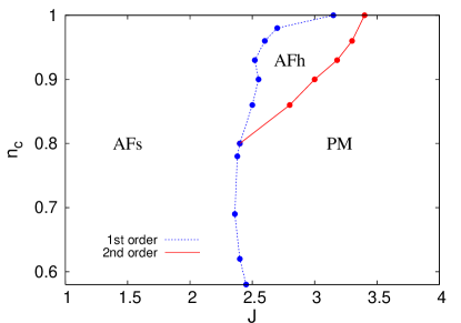
Figure 2: (Color on-line) Mean-field phase diagram. AFs and AFh indicate antiferromagnetic phases with small and hole-like Fermi surfaces, respectively. PM indicates a paramagnetic (metallic) phase. Continuous (dashed) lines mark second-order (first-order) phase transitions.

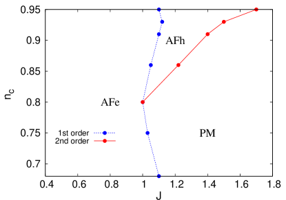
Figure 3: (Color on-line) Variational Monte Carlo phase diagram. The labels are the same as in Fig. 2. We note that, although qualitatively similar, the variational and mean-field phase diagrams are quantitatively quite different.

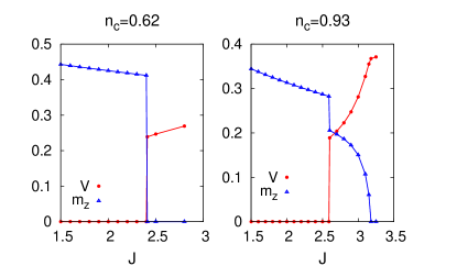
Figure 4: (Color on-line) Mean-field order parameters (hybridization $V$ and total magnetization $m_{z}=m_{f}-m_{c}$) as a function of the Kondo exchange for two different densities of the conducting electrons, $n_{c}=0.62$ (left panel) and $n_{c}=0.93$ (right panel).

III Results

Here we present our numerical results on the KLM, first within the mean-field approximation and then by the variational Monte Carlo approach.

III.1 Mean-field results

The mean-field phase diagram, as a function of $J$ and the electron density $n_{c}$, is reported in Fig. 2 (for a direct comparison, we report the variational Monte Carlo phase diagram in Fig. 3). For $n_{c}>0.81$ we find two distinct phase transitions. When $J$ is small, the ground state has antiferromagnetic long-range order and displays a small Fermi surface, namely we obtain the AFs state. Here, the local $f$ electrons are totally decoupled from the conducting ones (the mean-field equations are solved by $V=0$) and do not contribute to the Fermi surface. This regime is dominated by the RKKY interaction that generates a magnetic pattern in the localized spins, and consequently also in the conducting ones: the magnetization of $f$ electrons is saturated, i.e., $m_{f}=0.5$, while $m_{c}$ is a smooth function, slightly increasing with $J$.

By increasing $J$, the Kondo mechanism becomes competitive with the RKKY interaction and we enter into another antiferromagnetic phase, where $c$ and $f$ electrons are hybridized. Here, there is a hole-like Fermi surface and, therefore, the phase is AFh. The hybridization $V$ has a finite jump at the transition, which is, therefore, first order. In Fig. 4, we show the behavior of the hybridization $V$ and the total magnetization $m_{z}=m_{f}-m_{c}$. Eventually, by further increasing the local exchange, the Kondo mechanism prevails and the system becomes a paramagnetic metal where conduction electrons screen the local moments. The transition between the AFh phase and the paramagnetic metal is second order, with the magnetization that goes continuously to zero, see Fig. 4. Moreover, the hybridization is continuous though the transition and the topology of the Fermi surface does not change.

For smaller values of the conduction electron density, i.e., $n_{c}<0.81$, the AFh state cannot be stabilized and there are only two phases: the AFs for small Kondo exchange and the paramagnetic metal for large ones. The phase transition between them is first order: both the antiferromagnetic order parameter and the hybridization change abruptly from zero to a finite value, see Fig. 4. In this case, also the topology of the Fermi surface changes across the transition.

III.2 Variational Monte Carlo results

Now, we turn to the variational Monte Carlo results, summarized in the phase diagram of Fig. 3 (to be compared with the mean-field one, see Fig. 2). Within the variational Monte Carlo, which improves substantially the Hartree-Fock energy, the $c{-}f$ hybridization parameter $V$ of the non-interacting auxiliary Hamiltonian ${\cal H}_{\rm MF}$, is finite throughout the phase diagram. ogata It follows that the zero-temperature variational Fermi surface always includes both $c$ and $f$ electrons. However, the optimized $V$ is tiny in the AFe phase and steps up discontinuously entering the AFh or PM phases. Therefore, a very small temperature can wash away the effects of $V$ in the AFe phase (but not in the AFh and PM ones) thus better highlighting the differences between the phases. For this reason, we decided to follow Ref. lanata, and calculate, in the Brillouin zone, the emission spectrum $A(k)$ of ${\cal H}_{\rm MF}$ at the chemical potential broadened with a low but finite temperature $T$:

$$A(k)=-\int d\epsilon A(k,\epsilon)\frac{\partial f(\epsilon)}{\partial\epsilon},$$ (12)

where $A(k,\epsilon)$ is:

$$A(k,\epsilon)=\sum_{n>0}\,|\langle n|c^{\phantom{\dagger}}_{k,\sigma}|0\rangle|^{2}\delta(\epsilon-E_{n}+E_{0}),$$ (13)

where $|n\rangle$ are the unprojected (mean-field) states, with energies $E_{n}$.

We start our analysis by considering the paramagnetic sector, which is reacher than the one obtained within mean-field approximation, and can shed some light by disentangling Kondo effect from long-range magnetism. The paramagnetic phase diagram of the KLM, allowing for superconductivity, is shown in Fig. 5. We find that, although (on-site or extended) $s$-wave pairing is never stabilized, a sizable $d$-wave pairing is obtained in a wide range of parameters, namely for $J\lesssim 1.5$ and $n_{c}\gtrsim 0.65$, and brings a non-negligible energy gain with respect to a normal phase. The condensation energy is reported in Fig. 6 for three values of $n_{c}$. For $J\lesssim 0.1$, the pairing correlations of the unprojected state become very small, implying a tiny energy gain with respect to the normal state. We emphasize that superconductivity emerges only thanks to the electronic correlations brought by the Gutzwiller projector ${\cal P}_{f}$, since pairing does not arise at the mean-field level. A finite $d$-wave pairing is thus generated by the antiferromagnetic $c{-}f$ exchange, suggestive of similarities to analogous results found in $t{-}J$ models for cuprate superconductors. dagotto ; spanu Indeed, as evident from Fig. 6, the condensation energy has a bell-like shape, with maximum at some intermediate values of $J$ and $n_{c}$.

We mention that a very recent single-site dynamical mean-field theory (DMFT) calculation in the paramagnetic sector bodensiek finds evidence of $s$-wave superconductivity, whose maximum strength is reached, for a semicircular density of states, when $J\sim 1.6$ (translated in our units in which the bandwidth is $8t$) and $n_{c}\sim 0.86$, which we could not reproduce by our simple variational wave function.

In Fig. 7, we plot $A(k)$ for four different values of $J$, two well inside the superconducting region and two across the transition to the normal phase. Since the transition is continuous, the $T>0$ Fermi surface continuously change from electron-like to hole-like, see Fig. 7. A large spectral weight along the zone diagonals in the superconducting phase is observed whenever sizable pairing correlations are present, because of $d$-wave symmetry.

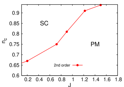
Figure 5: (Color on-line) Variational phase diagram in the paramagnetic sector. PM and SC denote the paramagnetic metal and the $d$-wave superconducting state, respectively. The transition between these two phases is always continuous.

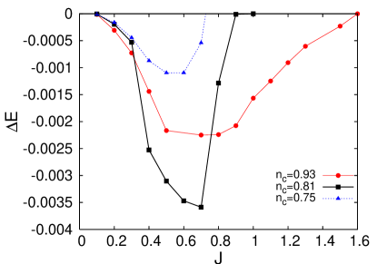
Figure 6: (Color on-line) Energy (per site) difference between the superconducting state and the metallic one as a function of $J$ for different values of the $c$-electron density.

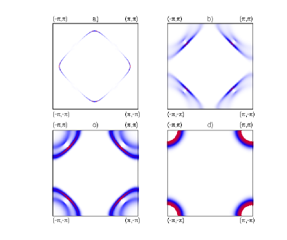
Figure 7: (Color on-line) Emission spectrum $A(k)$, see Eq. (12), broadened with a temperature $T=0.01$ for $n_{c}=0.91$. The top panels correspond to $J=0.2$ (left) and $J=0.8$ (right), the bottom one to $J=1.2$ (left) and $J=1.3$ (right). The lower three values of $J$ are inside the $d$-wave superconducting dome, while $J=1.3$ is already in the metallic phase. Note the change of topology as $J$ increases.

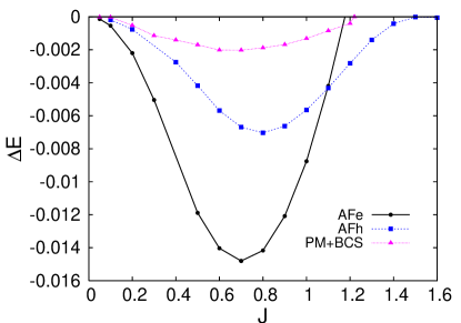
Figure 8: (Color on-line) Energy (per site) difference between the antiferromagnetic, superconducting, and normal states as a function of $J$ for $n_{c}=0.91$.

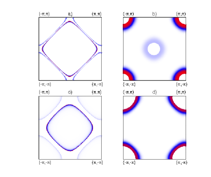
Figure 9: (Color on-line) Emission spectrum $A(k)$, see Eq. (12), broadened with a temperature $T=0.01$. Top left panel: $n_{c}=0.9375$ and $J=0.3$, inside the AFe phase. Top right panel: $n_{c}=0.9375$ and $J=1.3$, inside the AFh phase. Bottom left panel: $n_{c}=0.75$ and $J=0.2$, inside the AFe phase. Bottom right panel: $n_{c}=0.75$ and $J=1.2$, inside the PM phase. Note the shadow bands for the antiferromagnetic cases.

When we leave the paramagnetic sector and allow for antiferromagnetism, the latter prevails over superconductivity, which therefore disappear from the actual phase diagram, see Fig. 3. In other words, the energy gain of antiferromagnetism always overcomes that of superconductivity, see Fig. 8, ruling out the possibility of a ground state with superconductivity and no magnetic order. This occurs at least in the bipartite nearest-neighbor hopping model that we have considered, where the only source of frustration is the conduction electron density $n_{c}$ lower than half-filling. We also investigated possible coexistence between antiferromagnetism and $d$-wave superconductivity, which we indeed found but only in the AFe region. However, we believe this result is only a finite size effect, since the energy gain by allowing $d$-wave pairing on top of magnetism is tiny (at maximum, $\Delta E\simeq 10^{-4}t$) and, in addition, the size scaling of the actual order parameter (after Gutzwiller projection) suggests a vanishing value in the thermodynamic limit. We observe that the region of stability of the AFe phase is reduced substantially with respect to the corresponding AFs found at the mean-field level, compare Fig. 3 with Fig. 2, showing that the variational wave function can deal with Kondo screening better than mean field.

In Fig. 9 we draw $A(k)$ for different values of $n_{c}$ and $J$. The left panels are inside the AFe phase, and show a spectral distribution at the chemical potential that corresponds to a small, electron-like, Fermi surface. On the contrary, the right panels (the top one inside the AFh phase and the bottom one in the PM region) indicate a larger Fermi surface that still contains $f$ electrons at that value of temperature $T$. We note the signals of shadow bands in the antiferromagnetic $A(k)$ of the top panels and left bottom one.

We finally mention that the phase diagram of Fig. 3 agrees pretty well with that obtained by Watanabe and Ogata, ogata who also use a variational wave function similar to ours, though with less variational freedom since it allows only $c{-}f$ hybridization and antiferromagnetism. Indeed, we find that all additional variational parameters, e.g., $f{-}f$ hopping and superconductivity, do not change appreciably the energy, hence the phase diagram. Moreover, the variational phase diagram bears similarity also to that one obtained by Martin, Bercx, and Assaad assaad by the dynamical cluster approximation, although in the latter case all transitions seem continuous.

IV Conclusions

In conclusion, we have studied, by mean-field and variational Monte Carlo techniques, the Kondo lattice model on a square lattice. The mean-field phase diagram is qualitatively but not quantitatively similar to the variational Monte Carlo one. Restricting the analysis to the paramagnetic sector, we have found by variational Monte Carlo a large region of $d$-wave superconductivity, which however disappears from the phase digram once we allow for antiferromagnetism. It is well possible that, if magnetic frustration is added besides that due to $n_{c}<1$, superconductivity could emerge and intrude between the antiferromagnetic phase and the paramagnetic one, thus offering a possible explanation to what is observed in many heavy fermion compounds.

The variational Monte Carlo phase diagram is practically the same as that obtained by Watanabe and Ogata ogata by a similar technique. In particular we also find that the onset of antiferromagnetism and the breakdown of Kondo effect are not simultaneous close to compensation, $n_{c}=1$. Moreover, we find that the Kondo collapse always occurs via a first order phase transition and is accompanied by a redistribution of low-temperature spectral weight at the chemical potential inside the Brillouin zone.

- (1) S. Doniach, Physica B & C 91, 231 (1977).
- (2) G.R. Stewart, Rev. Mod. Phys. 73, 797 (2001).
- (3) H. Tsunetsugu, M. Sigrist, and K. Ueda, Rev. Mod. Phys. 69, 809 (1997).
- (4) C. Lacroix and M. Cyrot, Phys. Rev. B20, 1969 (1979).
- (5) F. Steglich, J. Aarts, C.D. Bredl, W. Lieke, D. Meschede, W. Franz, and H. Schafer, Phys. Rev. Lett. 43, 1892 (1979).
- (6) N.D. Mathur, F.M. Grosche, S.R. Julian, I.R. Walker, D.M. Freye, R.K.W. Haselwimmer, and G.G. Lonzarich, Nature (London) 394, 39 (1998).
- (7) S. Paschen, T. Luhmann, S. Wirth, P. Gegenwart, O. Trovarelli, C. Geibel, F. Steglich, P. Coleman, and Q. Si, Nature (London) 432, 881 (2004).
- (8) A. Schroder, G. Aeppli, R. Coldea, M. Adams, O. Stockert, H.V. Lohneysen, E. Bucher, R. Ramazashvili, and P. Coleman, Nature 407, 351 (2000).
- (9) P. Gegenwart, J. Custers, C. Geibel, K. Neumaier, T. Tayama, K. Tenya, O. Trovarelli, F. Steglich, Phys. Rev. Lett. 89, 056402 (2002).
- (10) J. Custers, P. Gegenwart, H. Wilhelm, K. Neumaier, Y. Tokiwa, O. Trovarelli, C. Geibel, F. Steglich, C. Pepin, and P. Coleman, Nature 424, 524 (2003).
- (11) P. Coleman, C. Pepin, Q. Si, and R. Ramazashvili, J. Phys.: Condens. Matter 13, R723 (2001).
- (12) S. Friedemann, T. Westerkamp, M. Brando, N. Oeschler, S. Wirth, P. Gegenwart, C. Krellner, C. Geibel, and F. Steglich, Nature Phys. 5, 465 (2009)
- (13) J. Custers, K.-A. Lorenzer, M. Mueller, A. Prokofiev, A. Sidorenko, H. Winkler, A.M. Strydom, Y. Shimura, T. Sakakibara, R. Yu, Q. Si, and S. Paschen, Nature Mat. 11, 189 (2012).
- (14) J.A. Hertz, Phys. Rev. B14, 1165 (1976).
- (15) A.J. Millis, Phys. Rev. B48, 7183 (1993).
- (16) A. Hack and M. Vojta, Phys. Rev. Lett. 106, 137002 (2011).
- (17) Q. Si, S. Rabello, K. Ingersent, and J.L. Smith, Nature (London) 413, 804 (2001).
- (18) T. Senthil, M. Vojta, and S. Sachdev, Phys. Rev. B69, 035111 (2004).
- (19) L. De Leo, M. Civelli, and G. Kotliar, Phys. Rev. B77, 075107 (2008).
- (20) H. Watanabe and M. Ogata, Phys. Rev. Lett. 99, 136401 (2007).
- (21) N. Lanatá, P. Barone and M. Fabrizio, Phys. Rev. B78, 155127 (2008).
- (22) L.C. Martin, M. Bercx, and F.F. Assaad, Phys. Rev. B82, 245105 (2010).
- (23) G.-M. Zhang and L. Yu, Phys. Rev. B62, 76 (2000).
- (24) S. Sorella, Phys. Rev. B71, 241103 (2005).
- (25) S. Sorella, G.B. Martins, F. Becca, C. Gazza, L. Capriotti, A. Parola, and E. Dagotto, Phys. Rev. Lett. 88, 117002 (2002).
- (26) L. Spanu, M. Lugas, F. Becca, and S. Sorella, Phys. Rev. B77, 024510 (2008).
- (27) O. Bodensiek, R. Zitko, M. Vojta, M. Jarrell, and T. Pruschke, arXiv:1301.5556.