Inhibition of the dynamical Casimir effect with Robin boundary conditions

Abstract

We consider a real massless scalar field in $3+1$ dimensions satisfying a Robin boundary condition at a nonrelativistic moving mirror. Considering vacuum as the initial field state, we compute explicitly the number of particles created per unit frequency and per unit solid angle, exhibiting in this way the angular dependence of the spectral distribution. The well known cases of Dirichlet and Neumann boundary conditions may be reobtained as particular cases from our results. We show that the particle creation rate can be considerably reduced (with respect to the Dirichlet and Neumann cases) for particular values of the Robin parameter. Our results extend for $3+1$ dimensions previous results found in the literature for $1+1$ dimensions. Further, we also show that this inhibition of the dynamical Casimir effect occurs for different angles of particle emission.

I Introduction

The dynamical Casimir effect (DCE) basically consists of the emission of quanta from a moving body in vacuum due to its interaction with a quantized field Moore-1970 ; Dewitt-PhysRep-1975 ; Fulling-Davies-PRS-1976-I ; Davies-Fulling-PRS-1977-I ; Davies-Fulling-PRS-1977-II . Another manifestation of the DCE, which is a direct consequence of the particle creation phenomenon if we invoke the energy conservation law, is a radiation reaction force acting on the moving body. This dissipative force gives rise to an irreversible exchange of energy between the moving body and the quantized field. In other words, the energy dissipated from the moving body is converted into real excitations of the quantized field, i.e., real particles. One can also understand the DCE in the opposite way, namely, from the fluctuation-dissipation theorem Nyquist-1928 ; Callen-Welton-1951 and from the fact that the static Casimir force acting on a fixed body, though zero, has non-vanishing fluctuations Barton91 . In this scenario, one expects that a moving plate may be acted by a dissipative force (under certain circumstances) which is proportional to the fluctuations of the Casimir force on the static plate Braginsky-Khalili-1991 ; Jaekel-Reynaud-1992 ; Barton94 (for the case of a moving sphere see Ref. MaiaNeto-Reynaud-1993 ).

However, the quantized field and the moving body can also exchange energy reversibly, which means that the force exerted on the moving body acquires in this case a dispersive part, as it occurs when Robin boundary conditions (BC) are considered Mintz-Farina-Maia-Neto-Robson-JPA-2006-I ; Farina-BJP-2006 . During the first two decades after the pioneering paper by Moore Moore-1970 , the calculations on the DCE were usually done with scalar fieds. The consideration of electromagnetic fields was made by the first time in 1994 MaiaNeto-1994 (see also Ref(s) MaiaNeto-Machado-1996 ; MaiaNeto-Mundurain-1998 ), and since then great attention has been devoted to the DCE. Detailed reviews on the DCE can be found in Refs. Dodonov-Revisao ; PAMN-EtAl-Revisao . Several experimental proposals to observe the DCE have been made in the last years. We shall briefly comment on a couple of them (for more details see, for instance, Dodonov’s paper V-V-Dodonov-Phys-Scrip-2010 ).

The so called motion induced radiation (MIR) experiment Braggio-Agnesi is based on the simulation of a mirror’s motion by changing the reflectivity of a semi-conductor by irradiating it with appropriate laser pulses, an ingenious idea firstly introduced by Yablonovitch in 1989 Yablonovitch-1989 in a paper where the main concern was to propose ways of simulating highly accelerated frames in order to enhance the Unruh radiation. A few years later, this same idea of creating a dense electron-hole plasma in a thin semiconductor by irradiating it with laser pulses, was also discussed by Lozovik et al LozovikEtAl-1995 . Though there are many promissing aspects in the MIR experiment, it is worth mentioning that the MIR experimentalists may have to deal with some difficulties. A first one is related to the limitations in the signal-to-noise ratio present in their experiment caused by thermal effects, in case they run the experiment at 4.6 K, as pointed out by Kim et al Kim-Brownell-Onofrio-EPL-2007 . A second one is the influence of damping in a parametric amplification process. And in the MIR experiment, the electric permittivity of the semiconductor slab after excitation by the laser pulse acquires a non-negligible imaginary part Dodonov-2005 , so that dissipation effects are inevitable. In this case, as shown by Dodonov, damping plays an important role and the emergence of a superchaotic quantum state may occur leading to a highly superPoissonian statistics for the distribution function of quanta Dodonov-2009 .

Another interesting proposal was made by Kim et al Kim-Brownell-Onofrio-PRL-2006 . They suggest that an indirect measurement of the dynamical Casimir photons generated by means of the mechanical motion of a film bulk acoustic resonator is detected with the aid of a superadiance mechanism. More recently, Dezael and Lambrecht Dezael-Lambrecht-EPL-2010 proposed that a (dynamical) Casimir-like radiation may arise from an effective motion of mirrors obtained by the interactions of an optical parametric oscillator with a thin non-linear crystal slab inside. In 2011, Kawakubo and Yamamoto Kawakubo-Yamamoto-PRA-2011 proposed that photons could be generated by means of a non-stationary plasma mirror, being the photons detectable by an excitation process of Rydberg atoms through the atom-field interaction. Still in 2011, Faccio and Carusotto Faccio-Carusotto-EPL-2011 proposed a photon generation mechanism in the near-infrared domain obtained by a train of laser pulses applied perpendicularly to a cavity, made of non-linear optical fiber, which modulates in time the refractive index of the medium filling the cavity.

Finally, forty years after its theoretical prediction made by Moore Moore-1970 , the first experimental observation of the DCE was announced by Wilson and collaborators C-Wilson-et-al-Nature-2011 , in an experiment where these authors use a superconducting circuit consisting of a unidimensional coplanar transmission line with a tunable electrical length. The change of the electrical length is performed by modulating the inductance of a superconducting quantum interference device fixed at one end of the transmission line. This modulation is achieved with the aid of a time-dependent magnetic flux through the superconducting quantum interference device. The electromagnetic field along the transmission line is described in terms of a field operator given by a scalar field $\phi(t,x)$ obeying a massless Klein-Gordon equation in 1+1 dimensions and submitted to a Robin BC with a time-dependent Robin parameter $\gamma(t)$ in the following manner J-R-Johansson-G-Johansson-C-Wilson-F-Nori-PRL-2009 :

$$\phi(t,0)\approx\gamma(t){(\partial_{x}\phi)}(t,0).$$ (1)

This kind of BC was also considered in Ref(s) Silva-Farina-PRD-2011 ; Farina-Silva-Rego-Alves-IJMPCS-2012 . In the context of the DCE, Robin BC appeared for the first time in the papers by Mintz and collaborators Mintz-Farina-Maia-Neto-Robson-JPA-2006-I ; Mintz-Farina-Maia-Neto-Robson-JPA-2006-II , who investigated a real massless scalar field $\phi(t,x)$ satisfying a Robin BC at a moving plate when observed from an inertial frame in which the plate is instantaneously at rest (we shall refer to this frame as tangential frame), according to the formula

$$\phi^{\prime}(t^{\prime},x^{\prime})=\gamma{(\partial_{x^{\prime}}\phi^{\prime})}(t^{\prime},x^{\prime}),$$ (2)

where the prime superscript is to remind us that the BC is taken in a tangential frame and $\gamma$ is now a time-independent Robin parameter.

For an oscillating mirror that imposes Dirichlet BC on a scalar field in $1+1$ dimensions, the total particle creation rate is a monotonic function of the mechanical frequency of the mirror Lambrecht-PRL-1996 . However, it was shown in Mintz-Farina-Maia-Neto-Robson-JPA-2006-II that this is not always the case when the field obeys a Robin BC given by Eq. (2). For a given value of $\gamma$, there is an interval in which an increase in the oscillation frequency of the mirror leads to a decrease in the particle emission. This can be understood as a kind of “decoupling” between the mirror and some of the field modes.

One important question that remains is whether or not this interesting effect still occurs in $3+1$ dimensions. This is not a trivial issue, once the phase space available for the field in $d=3+1$ is much larger than that in $1+1$ dimensions. To answer this question is the main purpose of our paper and we shall do that by considering a real massless scalar field in $3+1$ dimensions satisfying a Robin BC at a non-relativistic moving mirror (in the tangential frame). As far as we know, all papers about DCE with Robin BC deal with models in 1+1 dimensions, except one Diogo-Farina-Procceeding-2011 , which did not discuss the problem we are interested here.

An extra motivation to study this model is the connection between the DCE for a real massless scalar field in $3+1$ dimensions and the DCE for the electromagnetic field interacting with a perfectly conducting plate. The latter problem can be separated into two problems: a vector potential representing the transverse electric (TE) polarization, which is associated to a Dirichlet BC, and a vector potential representing the transverse magnetic (TM) polarization, which is associated to a Neumann BC. Since the parameter $\gamma$ allows a continuous interpolation between Dirichlet and Neumann BC, we expect that in the limit $\gamma\rightarrow 0$ the DCE for the massless scalar field coincides with the TE polarization contributionto the electromagnetic DCE, while for $\gamma\rightarrow\infty$ the TM polarization contribution to the electromagnetic DCE is recovered.

The structure of this paper is as follows. In Sec. II, we calculate the relations between the creation and annihilation field operators in the remote past (“in” operators) and in the far future (“out” operators), in the Heisenberg picture. In Sec. III, we show our results for the particle emission rate for a specific but typical motion of the mirror. Finally, in Sec. IV, we discuss our results and make a few comments on their possible consequences.

II Bogoliubov Transformation and Particle Spectrum

Let us consider - in the Heisenberg picture - a massless scalar field $\phi$ in $3+1$ dimensions written in terms of the time-dependent operators $a^{\dagger}(t,\bf k)$ and $a(t,\bf k)$, where ${\bf k}$ is the wave vector. In the distant past, these operators are relabeled as the creation and annihilation operators $a_{in}^{\dagger}({\bf k})$ and $a_{in}({\bf k})$, whereas in the far future they are relabeled as $a_{out}^{\dagger}({\bf k})$ and $a_{out}({\bf k})$. The time evolution of the operators $a^{\dagger}$ and $a$ depends on the interaction between the field with an external agent (modeled, in the present paper, by a moving boundary). The “out” operators can be expressed as a combination of the “in” operators via Bogoliubov transformations Bogoliubov

$$a_{out}({\bf k})=\alpha({\bf k})a_{in}({\bf k})+\beta({\bf k})a_{in}^{\dagger}({\bf k}),$$ (3)

where $\alpha$ and $\beta$ are named Bogoliubov coefficients. Assuming that in the remote past the system is in the vacuum state $|0\rangle$, the spectral density of the created particles after the movement of the mirror has ceased is given by

$$\frac{dN}{d^{3}k}({\bf k})=\frac{1}{\left(2\pi\right)^{3}}\langle 0|a_{out}^{\dagger}({\bf k})a_{out}({\bf k})|0\rangle=|\beta({\bf k})|^{2}.$$ (4)

Notice that there will be particle production if, and only if, $\beta({\bf k})\not=0$, i.e., if the annihilation operator $a_{out}({\bf k})$ is “contaminated” by the creation operator $a_{in}^{\dagger}({\bf k})$. The relation between the “in” and “out” operators can be calculated exactly for the case $1+1$ dimensions Davies-Fulling-PRS-1977-II with Dirichlet or Neumann BC. However, only approximate approaches are currently known for higher dimensional space-times. If the movement of the mirror is non-relativistic and has a small amplitude, the perturbative method introduced by Ford and Vilenkin Ford-Vilenkin-PRD-1982 applies. In the following, we will use the Ford-Vilenkin approach to find the Bogoliubov transformation for the massless scalar field satisfying the wave equation

$$\frac{\partial^{2}\phi}{\partial t^{2}}-\nabla^{2}\phi=0$$ (5)

and obeying a Robin BC imposed by a moving mirror. We start writing the field operator as the field under static BC plus a perturbation, that is

$$\phi(t,{\bf r})=\phi_{0}(t,{\bf r})+\delta\phi(t,{\bf r}),$$ (6)

where we assume that the undisturbed field $\phi_{0}$ obeys the static boundary condition BC

$$\Bigl{[}\phi_{0}\left(t,{\bf r}\right)-\gamma\partial_{z}\phi_{0}\left(t,{\bf r}\right)\Bigr{]}_{z=0}=0,$$ (7)

where $\gamma$ is a time-independent parameter.

The perturbation $\delta\phi$ (which is assumed to be small) gives the first order contribution to the total field $\phi(t,{\bf r})$ caused by the movement of the mirror and therefore will be responsible for the emergence of the DCE.

Let $z=\delta q(t)$ be the position of the mirror at a given instant. We assume that, in the lab reference frame, the mirror starts at rest at $z=0$, undergoes a given prescribed movement and finally settles down at $z=0$ for large times. The perturbation $\delta\phi$ will be small as long as the speed of the mirror is continuous with continuous derivatives and is much smaller than the speed of light, $|\delta\dot{q}(t)|\ll 1$, in natural units. Once we consider a bounded movement for the mirror, we also require that it possesses a small amplitude. More specifically, this means that $|\delta q|\ll 1/\omega_{0}$, where $\omega_{0}$ is the dominant mechanical frequency and this assumption will allow us to neglect terms ${\cal O}[(\delta q)^{2}]$, ${\cal O}[(\delta\phi)^{2}]$, ${\cal O}[\delta\phi\delta q]$ and ${\cal O}[(\delta\dot{q})^{2}]$.

We shall follow the same procedure as in Mintz-Farina-Maia-Neto-Robson-JPA-2006-II . At the tangential frame at a given instant, the BC is given by

$$\phi^{\prime}(t^{\prime},{\bf r}^{\prime})=\gamma^{\prime}\frac{\partial\phi^{\prime}}{\partial z^{\prime}}(t^{\prime},{\bf r}^{\prime}),$$ (8)

where $\gamma^{\prime}$ is a $t^{\prime}$-independent parameter. This BC can be cast in the lab frame with the help of the appropriate Lorentz transformations. For non-relativistic velocities, one may expand in first order in $\delta\dot{q}(t)$ to find

$$\Bigl{[}\partial_{z}\phi\left(t,{\bf r}\right)+\delta\dot{q}(t)\partial_{t}\phi\left(t,{\bf r}\right)-\gamma^{-1}\phi\left(t,{\bf r}\right)\Bigr{]}_{z=\delta q(t)}=0,$$ (9)

where, in this approximation, we consider that the Robin parameter is not affected by the Lorentz transformation, so that $\gamma^{\prime}=\gamma$.

We substitute (6) in (9) and expand the result thus obtained in the small parameters retaining only terms up to linear order in $\delta q$ and $\delta\phi$, finding

$$\partial_{z}\delta\phi\left(t,{\bf r}\right)|_{z=0}\;-\;\gamma^{-1}\delta\phi\left(t,{\bf r}\right)|_{z=0}\;\; = \;\;\delta q(t)\gamma^{-1}\partial_{z}\phi_{0}(t,{\bf r})|_{z=0}\;-\;\delta q(t)\partial_{z}^{2}\phi_{0}(t,{\bf r})|_{z=0}$$ (11)

$$\;-\;\delta\dot{q}(t)\partial_{t}\phi_{0}\left(t,{\bf r}\right)|_{z=0}.$$

Therefore, the perturbation $\delta\phi(t,{\bf r})$ obeys a time-dependent BC at a fixed position $(z=0)$, which is associated to the motion of the mirror via $\delta q(t)$.

It is now convenient that we express the field in the frequency domain using a Fourier transform, as follows. Let us define $\Phi(\omega,{\bf k}_{\parallel};z)$ as the Fourier transform of the field $\phi(t,{\bf r})$, so that

$$\Phi(\omega,{\bf k}_{\parallel};z):=\int_{-\infty}^{\infty}dt\int d^{2}{\bf r}_{\parallel}e^{i\omega t}e^{-i{\bf k}_{\parallel}\cdot{\bf r}_{\parallel}}\phi(t,{\bf r}).$$ (12)

Notice that $\Phi(\omega,{\bf k}_{\parallel};z)$ obeys the Helmholtz equation

$$\left(\omega^{2}-k^{2}_{\parallel}+\partial_{z}^{2}\right)\Phi(\omega,{\bf k}_{\parallel};z)=0.$$ (13)

Once the massless free scalar field is a solution of the d’Alembert equation (5),

$$k_{z}=\left[(\omega+i\epsilon)^{2}-k_{\parallel}^{2}\right]^{1/2},\;\;\text{with}\;\;\epsilon\rightarrow 0^{+}.$$ (14)

With this definition, $k_{z}$ is a complex function of $\omega$, with a branch cut along the real axis between $-k_{\parallel}<\omega<k_{\parallel}$ MaiaNeto-Machado-1996 , where $k_{\parallel}=|{\bf k}_{\parallel}|$.

The undisturbed field is the solution of the wave equation (5) subject to the static BC (7):

$$\phi_{0}(t,{\bf r}) = \int_{-\infty}^{\infty}d^{2}{\bf k}_{\parallel}\int_{0}^{\infty}dk_{z}\sqrt{\frac{1}{4\pi^{3}\left|\omega_{{\bf k}}\right|}\left(\frac{1}{1+\gamma^{2}k_{z}^{2}}\right)}\Biggl{[}a({\bf k})e^{-i\omega_{{\bf k}}t}e^{i{\bf k}_{\parallel}\cdot{\bf r}_{\parallel}}+a^{\dagger}({\bf k})e^{i\omega_{{\bf k}}t}e^{-i{\bf k}_{\parallel}\cdot{\bf r}_{\parallel}}\Biggr{]}\times$$ (16)

$$\Biggl{[}\sin(k_{z}z)+\gamma k_{z}\cos(k_{z}z)\Biggr{]},$$

where the field normalization is chosen so that the creation and annihilation operators obey the commutation relations

$$\left[a({\bf k}),a^{\dagger}(\bf k)^{\prime}\right]=(2\pi)^{3}\delta({\bf k}-{\bf k}^{\prime}).$$ (17)

We can now use (12) to write down the Fourier transform of the undisturbed field,

$$\Phi_{0}(\omega,{\bf k}_{\parallel};z) = A(\omega,k_{z};\gamma)\Bigl{[}\sin(k_{z}z)+\gamma k_{z}\cos(k_{z}z)\Bigr{]}\!\!\Bigl{[}a({\bf k})\Theta(\omega)-a^{\dagger}(-{\bf k})\Theta(-\omega)\Bigr{]}\Theta(k_{z}^{2}),\;\,$$ (18)

with the normalization factor

$$A(\omega,k_{z};\gamma)=\sqrt{\frac{16\pi^{3}\left|\omega\right|}{k_{z}^{2}}\left(\frac{1}{1+\gamma^{2}k_{z}^{2}}\right)}.$$ (19)

The Fourier transformations of the perturbation $\delta\phi(t,{\bf r})$ and the mirror’s law of motion $\delta q(t)$ are written as

$$\delta\Phi(\omega,{\bf k}_{\parallel};z)={\int_{-\infty}^{\infty}dt\int d^{2}{\bf r}_{\parallel}e^{i\omega t}e^{-i{\bf k}_{\parallel}.{\bf r}_{\parallel}}\delta\phi(t,{\bf r})}$$ (20)

and

$$\delta Q(\omega)={\int_{-\infty}^{\infty}dt\,e^{i\omega t}\delta q(t)}.$$ (21)

Notice that $\delta\Phi(\omega,{\bf k}_{\parallel};z)$ obeys the Helmholtz equation

$$\left(\omega^{2}-k^{2}_{\parallel}+\partial_{z}^{2}\right)\delta\Phi(\omega,{\bf k}_{\parallel};z)=0.$$ (22)

Recalling that we must take only the solution that propagates outwards from the moving mirror, the solution of the previous equation for $z>0$ is given by

$$\delta\Phi(\omega,{\bf k}_{\parallel};z)=\frac{1}{ik_{z}}\partial_{z}\delta\Phi(\omega,{\bf k}_{\parallel};0)e^{ik_{z}z}.$$ (23)

We now notice also that $\delta\Phi(\omega,{\bf k}_{\parallel};z)$ obeys the BC given by the Fourier transform of (11), namely,

$$\partial_{z}\delta\Phi(\omega,{\bf k}_{\parallel};0)-\gamma^{-1}\delta\Phi(\omega,{\bf k}_{\parallel};0) = \gamma^{-1}\int_{-\infty}^{\infty}\frac{d\omega^{\prime}}{2\pi}\delta Q(\omega-\omega^{\prime})\Bigl{[}\partial_{z}\Phi_{0}(\omega^{\,\prime},{\bf k}_{\parallel};0)+\Bigr{.}$$ (25)

$$\Bigl{.}\Bigl{(}\gamma\omega\omega^{\prime}-\gamma{\bf k}_{\parallel}^{2}\Bigr{)}\Phi_{0}(\omega^{\,\prime},{\bf k}_{\parallel};0)\Bigr{]}$$

Once the Fourier transform of the Ford-Vilenkin ansatz (6) is

$$\Phi(\omega,{\bf k}_{\parallel};z)=\Phi_{0}(\omega,{\bf k}_{\parallel};z)+\delta\Phi(\omega,{\bf k}_{\parallel};z),$$ (26)

we now need to find an expression for $\Phi(\omega,{\bf k}_{\parallel};z)$ that allows us to relate the Fourier transforms of the field in the remote past and distant future. This can be done straightforwardly by using Green’s functions, as in Mintz-Farina-Maia-Neto-Robson-JPA-2006-II .

Let us start with the one-dimensional version of Green’s identity, $\partial_{z}\{g[\partial_{z}f]-f[\partial_{z}g]\}=g[\partial_{z}^{2}f]-f[\partial_{z}^{2}g]$. We now identify the function $f$ in this formula as the perturbation $\delta\Phi$ and the function $g$ as the Green’s function of the Helmholtz operator, i.e., a function such that $\left(\omega^{2}-k^{2}_{\parallel}+\partial_{z}^{2}\right)g(\omega,{\bf k}_{\parallel};z,z^{\prime})=\delta(z-z^{\prime})$. After integration by parts, we can show that

$$\delta\Phi(\omega,{\bf k}_{\parallel};z^{\prime}) = \Bigl{[}g(\omega,{\bf k}_{\parallel};0,z^{\prime})\partial_{z}\delta\Phi(\omega,{\bf k}_{\parallel};0)\partial_{z}g(\omega,{\bf k}_{\parallel};0,z^{\prime})\delta\Phi(\omega,{\bf k}_{\parallel};0)\Bigr{]}.$$ (27)

We may freely define the Green’s function $g$ so that it obeys the Robin BC at the surface of the static mirror, i.e., $g(\omega,{\bf k}_{\parallel};0,z^{\prime})=\gamma\partial_{z}g(\omega,{\bf k}_{\parallel};0,z^{\prime})$. Then, the identity (27) leads to

$$\delta \!\Phi(\omega,{\bf k}_{\parallel};z^{\prime})g(\omega,{\bf k}_{\parallel};0,z^{\prime})\!\Bigl{[}\partial_{z}\delta\Phi(\omega,{\bf k}_{\parallel};0)-\gamma^{-1}\delta\Phi(\omega,{\bf k}_{\parallel};0)\!\Bigr{]}\;$$ (28)

and, using Eq. (25), we can write the perturbation as

$$\delta\Phi(\omega,{\bf k}_{\parallel};z^{\prime}) = \gamma^{-1}g(\omega,{\bf k}_{\parallel};0,z^{\prime})\int_{-\infty}^{\infty}\frac{d\omega^{\prime}}{2\pi}\delta Q(\omega-\omega^{\prime})\Bigl{[}\partial_{z}\Phi_{0}(\omega^{\,\prime},{\bf k}_{\parallel};0)+\Bigr{.}$$ (30)

$$\Bigl{.}\Bigl{(}\gamma\omega\omega^{\prime}-\gamma{\bf k}_{\parallel}^{2}\Bigr{)}\Phi_{0}(\omega^{\,\prime},{\bf k}_{\parallel};0)\Bigr{]}$$

Replacing (30) in (26) one finds

$$\Phi(\omega,{\bf k}_{\parallel};z^{\prime}) = \Phi_{0}(\omega,{\bf k}_{\parallel};z^{\prime})+\frac{1}{\gamma}g(\omega,{\bf k}_{\parallel};0,z^{\prime})\int_{-\infty}^{\infty}\frac{d\omega^{\prime}}{2\pi}\delta Q(\omega-\omega^{\prime})\Bigl{[}\partial_{z}\Phi_{0}(\omega^{\,\prime},{\bf k}_{\parallel};0)+\Bigr{.}$$ (32)

$$\Bigl{.}\Bigl{(}\gamma\omega\omega^{\prime}-\gamma{\bf k}_{\parallel}^{2}\Bigr{)}\Phi_{0}(\omega^{\,\prime},{\bf k}_{\parallel};0)\Bigr{]}.$$

The field $\Phi(\omega,{\bf k}_{\parallel};z^{\prime})$ can be written in two different forms. The first one involves $\Phi_{in}$, the Fourier transform of the unperturbed field $\phi_{0}(t,{\bf r}_{\parallel};z^{\prime})$ in the distant past, that is, the “in” field, to which we associate retarded Green’s functions. Then,

$$\Phi(\omega,{\bf k}_{\parallel};z^{\prime}) = \Phi_{\text{in}}(\omega,{\bf k}_{\parallel};z^{\prime})+\frac{1}{\gamma}g_{\text{ret}}(\omega,{\bf k}_{\parallel};0,z^{\prime})\!\int_{-\infty}^{\infty}\frac{d\omega^{\prime}}{2\pi}\delta Q(\omega-\omega^{\prime})\Bigl{[}\partial_{z}\Phi_{0}(\omega^{\,\prime},{\bf k}_{\parallel};0)+\Bigr{.}$$ (34)

$$\Bigl{.}\Bigl{(}\gamma\omega\omega^{\prime}-\gamma{\bf k}_{\parallel}^{2}\Bigr{)}\Phi_{0}(\omega^{\,\prime},{\bf k}_{\parallel};0)\Bigr{]},$$

where $\Phi_{\text{in}}(\omega,{\bf k}_{\parallel};z^{\prime})$ is the Fourier transform of $\phi_{\text{in}}(t,{\bf r})$, which is simply the unperturbed field at the remote past,

$$\phi_{0}(t,{\bf r})\mathop{\sim}_{t\rightarrow-\infty}\phi_{\text{in}}(t,{\bf r}).$$ (35)

Analogously, one can use advanced Green’s functions to express the field $\Phi_{0}(\omega,{\bf k}_{\parallel};z^{\prime})$ using the “out” field configuration, as follows,

$$\Phi(\omega,{\bf k}_{\parallel};z^{\prime}) = \Phi_{\text{out}}(\omega,{\bf k}_{\parallel};z^{\prime})+\frac{1}{\gamma}g_{\text{adv}}(\omega,{\bf k}_{\parallel};0,z^{\prime})\int_{-\infty}^{\infty}\frac{d\omega^{\prime}}{2\pi}\delta Q(\omega-\omega^{\prime})\Bigl{[}\partial_{z}\Phi_{0}(\omega^{\,\prime},{\bf k}_{\parallel};0)+\Bigr{.}$$ (37)

$$\Bigl{.}\Bigl{(}\gamma\omega\omega^{\prime}-\gamma{\bf k}_{\parallel}^{2}\Bigr{)}\Phi_{0}(\omega^{\,\prime},{\bf k}_{\parallel};0)\Bigr{]},$$

where $\Phi_{\text{out}}(\omega,{\bf k}_{\parallel};z^{\prime})$ is the Fourier transform of

$$\phi_{0}(t,{\bf r})\mathop{\sim}_{t\rightarrow\infty}\phi_{\text{out}}(t,{\bf r}).$$ (38)

From Eqs. (37) and (34), we can relate the “in” and “out” field operators through the advanced and retarded Green’s functions,

$$\Phi_{\text{out}}(\!\omega\!,{\bf k}_{\parallel};z^{\prime})\; = \;\Phi_{\text{in}}(\omega,{\bf k}_{\parallel};z^{\prime})\;+\frac{1}{\gamma}\Bigl{[}g_{\text{ret}}(\omega,{\bf k}_{\parallel};0,z^{\prime})-g_{\text{adv}}(\omega,{\bf k}_{\parallel};0,z^{\prime})\Bigr{]}\times$$ (40)

$$\!\int_{-\infty}^{\infty}\!\!\!\frac{d\omega^{\prime}}{2\pi}\delta Q(\omega-\omega^{\prime})\!\Bigl{[}\partial_{z}\Phi_{0}(\omega^{\,\prime},{\bf k}_{\parallel};0)+\!\Bigl{(}\gamma\omega\omega^{\prime}-\gamma{\bf k}_{\parallel}^{2}\Bigr{)}\Phi_{0}(\omega^{\,\prime},{\bf k}_{\parallel};0)\!\Bigr{]}\;$$

Using the solution (18) of the Helmholtz equation for the field subject to Robin BC, one can reexpress (40) as

$$\Phi_{\text{out}}(\omega,{\bf k}_{\parallel};z^{\prime}) = \Phi_{\text{in}}(\omega,{\bf k}_{\parallel};z^{\prime})+\left(\frac{2i}{1+\gamma^{2}k_{z}^{2}}\right)\Bigl{[}\sin(k_{z}z^{\prime})+\gamma k_{z}\cos(k_{z}z^{\prime})\Bigr{]}\times$$ (43)

$$\int_{-\infty}^{\infty}\frac{d\omega^{\prime}}{2\pi}A(\omega^{\prime},k_{z}^{\prime};\gamma)\delta Q(\omega-\omega^{\prime})k_{z}^{\prime}\Bigl{(}1-\gamma^{2}{\bf k}_{\parallel}^{2}+\gamma^{2}\omega\omega^{\prime}\Bigr{)}\times$$

$$\Bigl{[}a({\bf q})\Theta(k_{z}^{\prime})-a^{\dagger}(-{\bf q})\Theta(-k_{z}^{\prime})\Bigr{]}\Theta({k_{z}^{\prime 2}}),$$

where we defined

$${\bf q}:={\bf k}_{\parallel}+k_{z}^{\prime}\hat{z},$$ (44)

with

$$k_{z}^{\prime}=\left[(\omega^{\prime}+i\epsilon)^{2}-{\bf k}_{\parallel}^{2}\right]^{1/2}.$$ (45)

Once again, using (18) it is straighforward to show that

$$a_{\text{out}}\!(\!{\bf k}) = a_{\text{in}}({\bf k})+\frac{2ik_{z}}{\sqrt{\left|\omega\right|(1+\gamma^{2}k_{z}^{2})}}\int_{-\infty}^{\infty}\frac{d\omega^{\prime\prime}}{2\pi}{\sqrt{\frac{\left|\omega^{\prime\prime}\right|}{(1+\gamma^{2}k_{z}^{\prime\prime 2})}}}\delta Q(\omega-\omega^{\prime\prime})\Bigl{(}1-\gamma^{2}{\bf k}_{\parallel}^{2}+\gamma^{2}\omega\omega^{\prime\prime}\Bigr{)}\times$$ (47)

$$\Bigl{[}a_{\text{in}}({\bf q}^{\prime\prime})\Theta(k_{z}^{\prime\prime})-a_{\text{in}}^{\dagger}(-{\bf q}^{\prime\prime})\Theta(-k_{z}^{\prime\prime})\Bigr{]}\Theta({k_{z}^{\prime\prime 2}}),$$

with ${\bf q}^{\prime\prime}={\bf k}_{\parallel}+k_{z}^{\prime\prime}\hat{z}$. The last expression is a linear relation between the annihilation field operator in the far future with the creation and annihilation operators at the remote past. That is, (47) is the Bogoliubov transformation we were looking for.

As advertised, the vacuum state is annihilated by the “in” operator $a_{in}({\bf k})$, but not by the “out” operator $a_{out}({\bf k})$ due to the presence of $a_{in}^{\dagger}({\bf k})$ in the r.h.s. of (47). This clearly indicates a nonzero particle creation in $3+1$ dimensions due to the DCE for a massless field subject to Robin BC at a moving mirror.

After some straightforward manipulations, from Eq. (4) and using the Bogoliubov transformation (47), we can finally calculate the spectral density of created particles:

$$\frac{dN({\bf k})}{d^{3}{\bf k}} = \frac{A}{\left(2\pi\right)^{3}}\frac{4k_{z}^{2}}{|\omega|(1+\gamma_{0}k_{z}^{2})}\int_{|{\bf k}_{\parallel}|}^{\infty}\frac{d\omega^{\prime}}{2\pi}k_{z}^{\prime}\frac{|\delta Q(\omega+\omega^{\prime})|^{2}}{1+\gamma_{0}k_{z}^{\prime 2}}\Bigl{(}1-\gamma^{2}{\bf k}_{\parallel}^{2}-\gamma^{2}\omega\omega^{\prime}\Bigr{)}^{2},$$ (48)

where $A$ is the area of the moving plate. Taking into account the axial symmetry of the problem, it is interesting to rewrite (48) in terms of the variables

$$k_{z}=\omega\cos\theta\;\;\;\mbox{and}\;\;\;|{\bf k}_{\parallel}|=\omega\sin\theta,$$ (49)

with $\omega=|{\bf k}|$ and $\theta\in[0,\pi/2]$. Analogously, we have

$$k_{z}^{\prime}=\sqrt{\omega^{\prime 2}-{\bf k}_{\parallel}^{2}}=\sqrt{\omega^{\prime 2}-\omega^{2}\sin^{2}\theta},$$ (50)

which leads us to our expression for the particle spectrum per unit area, per unit solid angle

$$\frac{1}{A}\frac{dN}{d\omega d\Omega} = \frac{1}{\left(2\pi\right)^{3}}\frac{4\omega^{3}\cos^{2}\theta}{1+\gamma^{2}\omega^{2}\cos^{2}\theta}\int_{\omega\sin\theta}^{\infty}\frac{d\omega^{\prime}}{2\pi}\sqrt{\omega^{\prime 2}-\omega^{2}\sin^{2}\theta}\;\frac{|\delta Q(\omega+\omega^{\prime})|^{2}}{1+\gamma^{2}(\omega^{\prime 2}-\omega^{2}\sin^{2}\theta)}\times$$ (52)

$$\Bigl{(}1-\gamma^{2}\omega^{2}\sin^{2}\theta-\gamma^{2}\omega\omega^{\prime}\Bigr{)}^{2}.$$

The expression (52) is valid for an arbitrary motion of the mirror, as long as it is sufficiently slow ($|\delta\dot{q}|\ll 1$) and has a small amplitude. In the following section, we present our results for a specific but very useful law of motion, that of a mirror which oscillates, practically, at a single frequency.

III Results and Discussion

Let us consider that the movement of the mirror is described by

$$\delta q(t)=\epsilon_{0}\cos(\omega_{0}t)e^{-|t|/\tau},$$ (53)

which is a typical motion considered in investigations of the DCE MaiaNeto-Machado-1996 , where $\epsilon_{0}$ represents its amplitude, $\omega_{0}$ the dominating mechanical frequency and $\tau$ the effective time interval of the oscillation. The Fourier transform of Eq. (53) is

$$\delta Q(\omega)=\epsilon_{0}\tau\left[\frac{1}{1+(\omega+\omega_{0})^{2}\tau^{2}}+\frac{1}{1+(\omega-\omega_{0})^{2}\tau^{2}}\right].$$ (54)

In the limit with $\omega_{0}\tau\gg 1$, we obtain

$$|\delta Q(\omega)|^{2}\approx\frac{\pi}{2}\epsilon_{0}^{2}\tau[\delta(\omega-\omega_{0})+\delta(\omega+\omega_{0})],$$ (55)

which is reasonable once (54) possesses two narrow peaks around $\omega=\pm\omega_{0}$ in this limit. Substituting (55) into (52) and defining $\tilde{{\cal N}}$ the normalized particle spectrum per unit area, per unit time, per unit solid angle, given by

$$\tilde{{\cal N}}=\frac{1}{A}\frac{dN}{d\omega d\Omega}\left(\frac{\epsilon_{0}^{2}\tau}{8\pi^{3}}\right)^{-1},$$ (56)

we can write

$$\tilde{{\cal N}}(\omega,\omega_{0},\gamma,\theta)=\omega_{0}^{4}\;\cal{\tilde{F}}(\alpha,\beta,\theta)$$ (57)

where

$$\cal{\tilde{F}}(\alpha,\beta,\theta) = \frac{\alpha^{3}\cos^{2}\theta}{1+\alpha^{2}\beta^{2}\cos^{2}\theta}\sqrt{(\alpha-1)^{2}-\alpha^{2}\sin^{2}\theta}\frac{[1-\alpha^{2}\beta^{2}\sin^{2}\theta-\alpha\beta^{2}(1-\alpha)]^{2}}{1+\beta^{2}[(1-\alpha)^{2}-\alpha^{2}\sin^{2}\theta]}\times$$ (59)

$$\Theta[1-\alpha(1+\sin\theta)],$$

with $\alpha=\omega/\omega_{0}$ and $\beta=\omega_{0}\gamma$. Notice that the Heaviside function present in Eq. (57) indicates the following interesting features of the particle spectrum: particles associated to a certain frequency $\omega$ can be created in all angles if $0\leq\omega\leq\omega_{0}/2$; for particles associated to a frequency $\omega>\omega_{0}/2$, there is no particle emission for angles larger than $\theta_{0}(\omega)$, with

$$\theta_{0}(\omega)=\arcsin\left(\frac{\omega_{0}-\omega}{\omega}\right).$$ (60)

Moreover, observe that expression (57) coincides with the results found in MaiaNeto-Machado-1996 in two particular cases. In the limit $\gamma\rightarrow 0$, Eq. (57) reproduces the particle spectrum for TE photons, while for $\gamma\rightarrow\infty$ it corresponds to the spectrum of TM photons.

The normalized particle spectrum per unit area, per unit time, here labeled as ${\cal{N}}$, can be obtained by integrating (57) in the solid angle, with angular range $\theta\in[0,\pi/2]$:

$${\cal{N}}(\omega,\omega_{0},\gamma)=\omega_{0}^{4}\;{\cal{{F}}}(\alpha,\beta)$$ (61)

with

$$\;{\cal{F}}(\alpha,\beta)=2\pi\int_{0}^{\pi/2}\;d\theta\;\sin\theta\;\cal{\tilde{F}}(\alpha,\beta,\theta).$$ (62)

The results for $\omega_{0}=1$ and different values of $\gamma$ in ${\cal{N}}(\omega,\omega_{0},\gamma)$ are shown in Fig. 1. The spectrum is symmetric around $\omega_{0}/2$ for every value of $\gamma$. This is in agreement with the expectation that the particles are created in pairs with frequencies $\omega_{1}$ and $\omega_{2}$ so that $\omega_{1}+\omega_{2}=\omega_{0}$, the driving frequency of the mirror MaiaNeto-Machado-1996 .

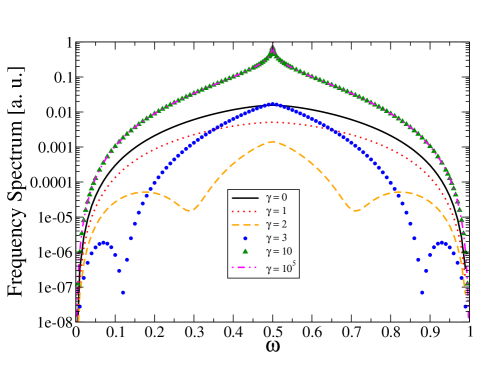
Figure 1: (Color online.) The normalized spectrum ${\cal N}$ in arbitrary units, as function of $\omega$, for different values of $\gamma$, with $\omega_{0}=1$. The particle emission at a given frequency $\omega$ is initially reduced as $\gamma$ increases from zero until a given angle and then it starts increasing, reaching a fixed plateau for $\gamma\rightarrow\infty$.

One can also analyze the angular spectrum of emitted particles. Our results for $\cal{\tilde{N}}$, which follow from Eq. (57) for a particular frequency $\omega=\omega_{0}/2$ and $\omega_{0}=1$, are shown in Fig. 2. A few comments are in order. Firstly, for small values of the Robin parameter, $\gamma\lesssim 1$, the emission is mainly forward, with large angle emission being suppressed. In second place, for $\gamma\simeq 2$, the emission is strongly inhibited for every angle, but it also acquires a maximum around $\theta\simeq 1$rad. If the $\gamma$ is further increased, the emission rate rises again as a whole, but the particle production is highest around $\theta\simeq 1$rad, and not around the normal direction $\theta=0$. Another interesting and subtle point becomes evident when we compare the angular spectrum in the case of Robin boundary conditions with $\gamma\gg 1$ and that of the Neumann BCs. We see from Fig. 2 that there is no emission for $\theta\rightarrow\pi/2$ no matter how large the values of $\gamma$ are. This is basically due to the factor $\cos^{2}\theta$ in (57). However, as shown in MaiaNeto-Machado-1996 , there is a finite emission rate at $\theta\rightarrow\pi/2$ for Neumann BC. The apparent paradox can be solved by noticing that the limits $\theta\rightarrow\pi/2$ and $\gamma\rightarrow\infty$ in Eq. (52) do not commute. Fortunately, this subtlety affects only grazing angles and the limit $\gamma\rightarrow\infty$ can be identified with the Neumann BC whenever $\theta=\pi/2$ is not the only angle in consideration.

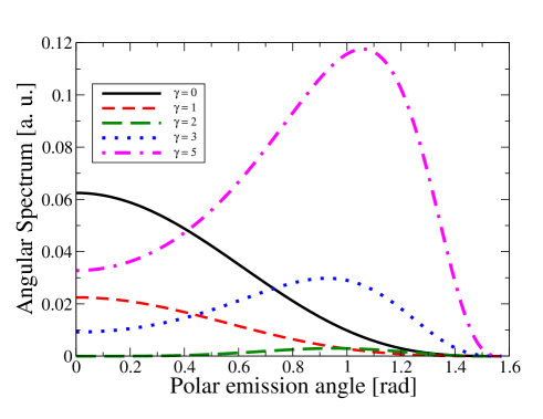
Figure 2: (Color online.) Angular spectrum ${\cal{\tilde{N}}}$ of emitted particles with frequency $\omega=\omega_{0}/2$, with $\omega_{0}=1$, as a function of the emission angle (measured with respect to the normal to the mirror) for various values of $\gamma$. Solid (black) line: $\gamma=0$; dashed (red) line: $\gamma=1$; long dashed (green) line : $\gamma=2$; dotted (blue) line: $\gamma=3$; dashed-dotted (magenta) line: $\gamma=5$.

Finally, let us turn our attention to the total number of particles emitted $N$, which is given by

$$N(\omega_{0},\gamma)=\omega_{0}^{5}\;F(\beta)$$ (63)

where

$$F(\beta)=\int_{0}^{\infty}\;d\alpha\;{\cal F}(\alpha,\beta).$$ (64)

The ratio between the emission rate $N_{R}=N(\omega_{0},\gamma)$ and the emission rate $N_{D}=N(\omega_{0},0)$ (Dirichlet BC), is given by

$$N_{R}/N_{D}=F(\beta)/F(0),$$ (65)

which is showed in Fig. 3. As first demonstrated in MaiaNeto-Machado-1996 , the total emission rate for Neumann BC is 11 times larger than that for Dirichlet BC in $3+1$ dimensions. Our results not only confirm the factor 11 but also show that Dirichlet and Neumann cases are connected by a non-monotonic curve. Indeed, the Robin BC with $\gamma\omega_{0}\simeq 2$ provides a very strong inhibition of the particle production. This property of the DCE with Robin BC had already been noticed in $1+1$ dimensions Mintz-Farina-Maia-Neto-Robson-JPA-2006-II , but it was not obvious a priori that this property would be preserved at higher dimensions.

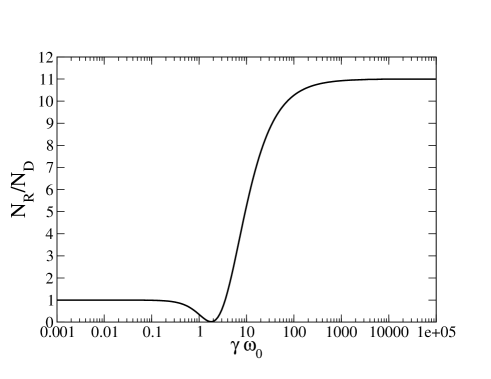
Figure 3: (Color online.) Total emission rate for Robin BC normalized by the Dirichlet rate. Notice that the Neumann limit ($\gamma\rightarrow\infty$) is correctly recovered. The strong decoupling between the mirror and the quantum vacuum field at $\gamma\omega_{0}\simeq 2$ is typical of the Robin BC Mintz-Farina-Maia-Neto-Robson-JPA-2006-I ; Mintz-Farina-Maia-Neto-Robson-JPA-2006-II .

IV Final remarks

We have investigated the DCE for a real massless scalar field in $3+1$ dimensions satisfying a Robin BC at a non-relativistic moving plate (in the tangential frame). We used the perturbative method of Ford and Vilenkin Ford-Vilenkin-PRD-1982 , valid for non-relativistic motions of small amplitudes to evaluated the Bogoliubov transformations between creation and annihilation operators in the remote past, $a_{in}$, and distant future, $a_{out}$. This allowed us to determine the spectral and angular distributions of the created particles caused by the moving mirror. Eq. (52) exhibits our expression for the particle spectrum per unit area, valid for a general (non-relativistic) law of motion for the moving plate. Assuming the oscillating law of motion given by Eq. (53) - a typical motion considered in investigations of the DCE - we obtained an explicit expression for the spectrum per unit area, given by Eq. (57). In the limit $\gamma\rightarrow 0$ (Dirichlet case) we recovered the particle spectrum for TE photons, whereas for $\gamma\rightarrow\infty$ (Neumann case) we reobtained the spectrum of emitted TM photons.

Our results also show that, although in the limits $\gamma\rightarrow 0$ and $\gamma\rightarrow\infty$ the total number of created particles is a monotonic function of the mechanical frequency of the plate, $\omega_{0}$, the same is not true for intermediate values of $\gamma$. In fact, for any fixed positive $\gamma$, the total number of created particles is not a monotonic function of $\omega_{0}$. More than that, the strong inhibition of the DCE that occurs in $1+1$ dimensions, when the Robin BC is present, also occurs in $3+1$ dimensions. Indeed, the total number of created particles shown in Fig. 3 is dramatically reduced for a quasi-harmonic motion with a frequency $\omega_{0}$ such that $\gamma\omega_{0}\simeq 2$, where $\gamma$ is the parameter that characterizes the Robin condition. Naively thinking, this surprising effective decoupling between the plate and the quantized field, predicted previously in $1+1$ dimensions Mintz-Farina-Maia-Neto-Robson-JPA-2006-I ; Mintz-Farina-Maia-Neto-Robson-JPA-2006-II was not expected in $3+1$, since in the latter case only the field modes that propagates perpendicularly to the plate are expected to behave as the field modes in $1+1$ dimensions.

The suppression just discussed show how the dynamical Casimir effect may be strongly dependent on the boundary conditions employed. This fact is very important, since any extra information about the created particles, either in the total number of them or in the angular dependence of the corresponding spectral distribution, can be extremely useful to better identify the dynamical Casimir photons in a given experiment. Since the Robin parameter $\gamma$ can be interpreted as the plasma wavelength of a given material, the results presented here may be of some help for future experiments, at least as a source of concern and caution when dimensioning these experiments. For the moment, realistic values for the product $\gamma\omega_{0}$ are still very far from a strong suppression, but this may not be the case in future experiments. It would be interesting if the peculiar signature of the DCE with Robin conditions - the strong inhibition in the particle emission - could eventually be captured in experiments. Considering the connections between Robin BC and the theoretical model underlying the first experimental observation of the DCE C-Wilson-et-al-Nature-2011 , we believe that a thorough study of the implications of the Robin boundary conditions on the DCE is crucial.

As a final comment, since the dissipative force acting on a moving mirror is closely related to the particle creation, we expect that this dissipative force will also suffer a similar inhibition in $3+1$ dimensions, as it occurs in the $1+1$ dimensional case Mintz-Farina-Maia-Neto-Robson-JPA-2006-I . This calculation will be left for a future work.

References

- (1) G.T. Moore, J Math. Phys. 11, 2679 (1970).
- (2) B.S. DeWitt, Phys. Rep. 19, 295 (1975).
- (3) S.A. Fulling and P.C.W. Davies, Proc. R. Soc. London, A 348, 393 (1976).
- (4) P.C.W. Davies and S.A. Fulling, Proc. R. Soc. London, A 354, 59 (1977).
- (5) P. C. W. Davies and S. A. Fulling, Proc. R. Soc. London, A 356, 237 (1977).
- (6) H. Nyquist, Phys. Rev. 32, 110-113 (1928).
- (7) H.B. Callen and T.A. Welton, Phys. Rev. 83, 34 (1951).
- (8) G. Barton, J. Phys. A: Math. Gen. 24, 991 (1991).
- (9) V.B. Braginsky and F.Ya. Khalili, Phys. Lett. 161, 197 (1991).
- (10) M.T. Jaekel and S. Reynaud, Quant. Opt. 4, 39 (1992).
- (11) G. Barton, in Cavity Quantum Electrodyamics, Supplement: Advances in Atomic, Molecular and Optical Physics, edited by P. Berman, (Academic Press, New York, 1993).
- (12) P.A. Maia Neto and S. Reynaud, Phys. Rev. A 47, 1639 (1993).
- (13) B. Mintz, C. Farina, P.A. Maia Neto and R.B. Rodrigues, J. Phys. A 39, 6559 (2006).
- (14) C. Farina, Braz. J. Phys. 36, 1137 (2006).
- (15) P.A. Maia Neto J. Phys. A 27, 2167 (1994).
- (16) P.A. Maia Neto and L.A.S. Machado, Phys. Rev. A 54, 3420 (1996).
- (17) D.F. Mundarain and P.A. Maia Neto, Phys. Rev. A 57, 1379 (1998).
- (18) V.V. Dodonov, Adv. Chem. Phys. 192, 309 (2001).
- (19) D.A.R. Dalvit, P.A. Maia Neto and F.D. Mazzitelli, in Casimir Physics, edited by D.A.R. Dalvit, P. Milonni, D. Roberts and F. da Rosa, Lecture Notes in Physics, Vol. 834 (Springer, New York, 2011).
- (20) V.V. Dodonov, Phys. Scrip. 82, 038105 (2010).
- (21) C. Braggio et al, Europhys. Lett 70, 754 (2005); A. Agnesi et al, J. Phys. A 41, 164024 (2008); A. Agnesi et al, J. Phys: Conf. Series 161, 012028 (2009).
- (22) E. Yablonovitch, Phys. Rev. Lett. 62, 1742 (1989).
- (23) Yu.E. Losovik, V.G. Tsvetus and E.A. Vinogradov, JETP Lett. 61 723 (1995).
- (24) W.-J. Kim, J.H. Brownell and R. Onofrio , Europhys. Lett 78, 21002 (2007).
- (25) V.V. Dodonov, J. Opt. B 7, S445 (2005).
- (26) V.V. Dodonov, Phys. Rev. A 80, 023814-1 (2009).
- (27) W.J. Kim, J.H. Brownell and R. Onofrio , Phys. Rev. Lett. 96, 200402 (2006).
- (28) F.X. Dezael and A. Lambrecht, Eur. Phys. Lett. 89, 14001 (2010).
- (29) T. Kawakubo and K. Yamamoto, Phys. Rev. A, 83, 013819 (2011).
- (30) D. Faccio and I. Carusotto, Eur. Phys. Lett 96, 24006 (2011).
- (31) C. M. Wilson, G. Johansson, A. Pourkabirian, M. Simoen, J. R. Johansson, T. Duty, F. Nori and P. Delsing, Nature, 479, 376 (2011).
- (32) J.R. Johansson, G. Johansson, C.M. Wilson and F. Nori, Phys. Rev. Lett. 103, 147003 (2009).
- (33) Hector O. Silva and C. Farina, Phys. Rev. D, 84, 045003 (2011).
- (34) C. Farina, Hector O. Silva, Andreson L. C. Rego and Danilo T. Alves, Int. J. Mod. Phys. Conf. Ser., 14, 306 (2012).
- (35) B. Mintz, C. Farina, P.A. Maia Neto and R.B. Rodrigues, J. Phys. A 39, 11325 (2006).
- (36) A. Lambrecht, M.-T. Jaekel and S. Reynaud, Phys. Rev. Lett. 77, 615 (1996).
- (37) Diogo Azevedo, F. Pascoal and C. Farina in: Proceedings of the IX Workshop on Quantum Field Theory under the Influence of External Conditions, edited by K.A. Milton and M. Bordag, (World Scientific, Singapore, 2009).
- (38) N. N. Bogoliubov, Sov. Phys. JETP, 7, 51 (1958).
- (39) L.H. Ford and A. Vilenkin, Phys. Rev. D 25, 2569 (1982).