An Algorithm for Precise Aperture Photometry of Critically Sampled Images

Abstract

We present an algorithm for performing precise aperture photometry on critically sampled astrophysical images. The method is intended to overcome the small-aperture limitations imposed by point-sampling. Aperture fluxes are numerically integrated over the desired aperture, with sinc-interpolation used to reconstruct values between pixel centers. Direct integration over the aperture is computationally intensive, but the integrals in question are shown to be convolution integrals and can be computed $\gtrsim 10000\times$ faster as products in the wave-number domain. The method works equally well for annular and elliptical apertures and could be adapted for any geometry. A sample of code is provided to demonstrate the method.

1 Introduction

In aperture photometry, one seeks to measure the flux which would have been received had the light passed through a physical aperture (e.g. a photomultiplier tube). An aperture flux in an astrophysical image is typically measured as the sum of the pixel fluxes for pixels near a given source. The region summed over is the ‘aperture’, and may contain whole and/or partial or weighted pixels. Circular apertures are common for astrophysical measurements, and are implemented in some form in most standard software packages, including IRAF (Tody 1986), DAOPHOT (Stetson 1987), and SExtractor (Bertin & Arnouts 1996).

Aperture fluxes are most commonly used in calibration when constructing a ‘growth curve’. A growth curve plots the enclosed flux within an aperture as a function of its radius, and is essential for calibrating fluxes measured through an optimal (typically small) aperture to bright isolated standard stars which must be measured with a large aperture to include all flux. Also, a number of commonly used flux measurements are aperture fluxes computed for scientifically interesting aperture shapes or sizes. Examples include Kron fluxes (Kron 1980) and Petrosian fluxes (Petrosian 1976).

For aperture radii comparable to the pixel dimensions, if no partial pixels are used, the ‘circular’ aperture can be quite non-circular (e.g. a $1\times 1$ or $2\times 2$ square, a cross, etc.). As the flux may change significantly across a pixel, the use of geometric partial pixels (e.g. including 0.5$\times$flux for a pixel with half of its area enclosed in the aperture) will not accurately represent the flux contained in the corresponding fraction of the pixel. To maintain a truly constant aperture geometry (circular or otherwise), the flux must be interpolated between pixels and integrated.

Here we describe a straightforward aperture photometry algorithm, which under normal observing conditions preserves circular aperture geometry perfectly and remains well-defined to arbitrarily small radii. For the method to be accurate, the pixels must critically sample the point-spread function (PSF); i.e. the spatial frequency of the pixels must be at least twice the highest spatial frequency present in the PSF. The method works equally well for annular and elliptical apertures, and could be adapted for any desired shape. The ability to handle elliptical apertures, in particular, makes it useful for computing Kron and elliptical Petrosian fluxes. It is implemented in the image processing pipeline under development for the Large Synoptic Survey Telescope (LSST) (Ivezic et al. 2008).

To compute the flux that would have been received through a truly circular aperture centred on a point source, we perform a continuous reconstruction of the discretely sampled pixel fluxes (Section 2) and integrate to yield the circular aperture flux (Section 3). The two-dimensional integral is computationally intensive, but we use Fourier methods to compute it quickly without loss of precision (Section 4). In Section 5, we modify the method to compute annular and elliptical apertures; and in Section 6 we evaluate the performance of the algorithm by comparing growth curves for model point-spread functions (PSFs) to their known values. Results are discussed and summarized in Sections 7 and 8, respectively. Some additional calculations are included in Appendix A, and an example program (written in Python) is included in Appendix B.

2 Reconstructing a Discretely Sampled PSF

A telescope produces a continuous function and delivers it to a detector, which convolves with the pixel response and point-samples it. In our technique, we use the sampling theorem to recover the continuous function, and measure it. Our only assumption is that the function must be band-limited. In this context, this implies that the Fourier transform of the PSF has negligible power above the Nyquist wave number which corresponds to the pixel sampling.

The sampling theorem states that a discretely sampled continuous function can be completely represented by its samples. In one dimension

$$p(x)=\sum_{i}\ p_{i}\ \frac{\sin(\pi(x-x_{i}))}{\pi(x-x_{i})}.$$ (1)

Equation 1 can be used to interpolate $p(x)$ given the discrete samples $p_{i}$. As the $\sin(x)/x$ term is a $\mathrm{sinc}$ function, this is known as $\mathrm{sinc}$ interpolation. Figure 1 demonstrates how the sinc interpolation of a one-dimensional PSF can be understood in terms of Fourier methods. If the sampled function is truly band-limited (no power above the Nyquist wave number), the $\mathrm{sinc}$ interpolation is an exact representation of the underlying continuous function. The proof of the sampling theorem can be found in the original work by Shannon (1949).

Figure 1: The sinc interpolation of a one-dimensional PSF. A discretely sampled PSF (a) is transformed with a discrete Fourier transform (b), and truncated at the Nyquist wave number (c). This truncation is the product of a boxcar and the wave-number coefficients, and is therefore represented by the convolution of a $\mathrm{sinc}$ (the Fourier transform of a boxcar) with the sampled points in real space (d). If the sampled function is truly band limited, the $\mathrm{sinc}$ representation shown as a dashed line in (d) is exact.

The sinc decomposition of a two-dimensional function has the form

$$p(x,y)=\sum_{j}\sum_{i}\ p_{ij}\ \frac{\sin(\pi(x-x_{i}))}{\pi(x-x_{i})}\ \frac{\sin(\pi(y-y_{j}))}{\pi(y-y_{j})}.$$ (2)

2.1 Testing the Band-Limit of a Gaussian PSF

The requirements for the $\mathrm{sinc}$ reconstruction to be valid are that the PSF be band limited, and that an infinite sequence of values are available. However, in both cases more practical limits are sufficient. Here we test the first assumption (the band limit) in the context of reconstructing a continuous PSF. Requirements on the extent of the data are dealt with in Section 3.1.

The validity of the band-limit assumption was verified by evaluating the error in integrated flux as a function of the sampling interval. This was estimated analytically with a circular bivariate single-Gaussian PSF model, and also measured numerically with a double-Gaussian PSF. A PSF is typically well-modeled by a double Gaussian (a sum of two bivariate Gaussians, one modeling the PSF core and the other modeling the wings). The single-Gaussian model used for the analytic estimate is intended to test the core Gaussian of a double-Gaussian PSF. If the ‘band limit’ criterion is satisfied for the narrower Gaussian, it would easily be satisfied for the larger one representing the wings.

For our analytic model, the calculation of the fractional error due to aliased power in a sampled Gaussian is a straightforward exercise, and is presented in Appendix A. The resulting upper-limit estimate for the fractional flux error is

$$\frac{\mathrm{error}}{\mathrm{total\ flux}}=\frac{e^{-\pi^{2}\sigma^{2}/2}}{2\pi^{1/2}\sigma}.$$ (3)

To verify the method more rigorously, it was also tested numerically with known PSFs. For the numerical tests, the so-called ‘double Gaussian’ is a reasonable approximation to a typical observed PSF. Our double-Gaussian test PSF has core and wing components, with the wing component having 10% of the core’s amplitude and a width of $\sigma_{\mathrm{wing}}=2\sigma_{\mathrm{core}}$. A double Gaussian also has the advantage that it can be integrated analytically to provide an exact known flux for comparison to the $\mathrm{sinc}$-integrated value, and it was therefore used for these numerical tests.

The response of the pixel is considered to be a part of the PSF structure (i.e. the continuous PSF produced by the telescope is convolved with a pixel and then point-sampled by the detector), and the double Gaussian model used in the numerical tests was directly point-sampled. As convolving a Gaussian with a pixel is very close to convolving with a another Gaussian having $\sigma=1/\sqrt{12}$, the resulting function remains very close to a Gaussian.

Both theoretical (equation 3) and numerically measured errors are shown as a function of the PSF size in pixels (i.e., the sampling) in Figure 2. An aperture with a radius of 6 pixels was used. For the numerical tests, sub-pixel centroid shifts were applied to verify the method for PSF profiles that are not centred at integer pixel positions, and representative curves corresponding to shifts of $(\delta_{x},\delta_{y})$ = $(0.0,0.0)$; and $(0.5,0.5)$ are presented. Provided the PSF’s $\sigma_{\mathrm{core}}$ is larger than $\sim$1 pixel (corresponding to a FWHM $\gtrsim 2.5$ pixels for a double Gaussian), fractional flux errors due to undersampling are $\ll$ 0.001, or $\sim$1 mmag.

Figure 2: The flux error due to truncation/aliasing of wave numbers with $q>\pi$ as a function of PSF size in pixels for a double Gaussian (lower panel), with the absolute value shown in the upper panel. The flux error is $1-$measured/true, where ‘measured’ refers to our $\mathrm{sinc}$-integration algorithm (aperture radius of 6 pixels), and ‘true’ refers to the exact integral of the double Gaussian (sum of circular bivariate Gaussians having different amplitudes (wing being 10% of core) and widths ($\sigma_{\mathrm{wing}}=2\sigma_{\mathrm{core}}$)). Curves are shown for a double Gaussian centred on an integer pixel value (solid), and one shifted by 0.5 pixels (dashed). Limits based on our conservative theoretical estimate are shown with dot-dashed lines. The theoretical estimate is the limit for truncated flux, while the $\mathrm{sinc}$-integrated curves include aliased flux. Dotted lines indicate a fractional error of 0.001, or $\sim$1 mmag. For the Gaussian PSFs, the flux error is $\ll 1$mmag provided sampling is $\sigma\gtrsim 1$ pixel. In cases of severe undersampling, the formalism of including the pixel response in the double-Gaussian PSF breaks down; therefore, values for small PSF widths ($\sigma_{\mathrm{core}}<0.4$ pixels) are not shown.

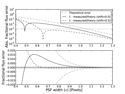
It is tempting to assume that any error introduced through aliasing would be systematic and correspond to a fractional excess or deficit of flux. Such an error could be corrected by calibrating the measured fluxes against standard stars. However, Figure 2 shows that the errors are different for the $(\delta_{x},\delta_{y})$ = $(0.0,0.0)$; and $(0.5,0.5)$ pixel shifts. In general, the error for each measured source depends on the sub-pixel shift of the PSF and cannot be corrected through calibration. Further, galaxies and other non-point-sources will be composed of different spatial frequencies and their errors will be different from those of point sources and from other galaxies.

If the method is to be used in the construction of a growth curve (flux measurements at a series of progressively larger apertures), the band-limited nature of the PSF must be taken seriously as the error is a function of radius and can be large for undersampled PSFs. For additional information, see Section 6.1 where the performance of the method is tested directly by measuring growth curves.

With these caveats in mind, a double-Gaussian PSF is band limited for the pixel scales and aperture sizes commonly used in astronomy ($\sigma>1$ pixel, or FWHM $>2.5$ pixels).

3 Computing Aperture Flux

With the discrete pixel fluxes, $p_{ij}$, interpolated to form a continuous function, $p(x,y)$ (see equation 2), a precise aperture flux, $f_{A}$, can be obtained by integrating over the desired aperture $A$:

$$f_{A}=\iint\limits_{A}\ p(x,y)\ \mathrm{d}x\mathrm{d}y.$$ (4)

The integration can be performed to arbitrary precision, but depending on the structure of the aperture, and integrator used, it may be computationally intensive (recall that the $p(x,y)$ function is a sum of $\mathrm{sinc}$ functions – one for each pixel).

Fortunately, the $p_{ij}$ terms in equation 2 are constant and can be factored out of the integral in equation 4, allowing the aperture flux to be expressed as a weighted sum:

$$f_{A}=\sum_{j}\sum_{i}\ w_{ij}\ p_{ij},$$ (5)

where the weighting terms are

$$w_{ij}=\iint\limits_{A}\ \frac{\sin(\pi(x-x_{i}))}{\pi(x-x_{i})}\ \frac{\sin(\pi(y-y_{j}))}{\pi(y-y_{j})}\ \mathrm{d}x\ \mathrm{d}y.$$ (6)

Thus, for each pixel we compute a corresponding weight, $w_{ij}$, in the sum for the aperture flux. The integral ($w_{ij}$) does not depend on $p_{ij}$. It can be computed once and shifted (see Section 4.1) to be applied to different sources in a given frame. This is critical for efficiency. Without the ability to pre-compute the $w_{ij}$ coefficients, several numerical integrals would need to be computed for each source being measured, and the method would be prohibitively slow.

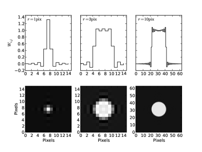
For a large circular aperture, pixels near the center have weight $w_{ij}\approx 1$. Near the edge of the aperture, values transition from $\sim$1 to $\sim$0. However, values outside the aperture do not go completely to 0. Some non-zero weight remains even several pixels outside the aperture radius. Examples of $w_{ij}$ coefficients for different-sized circular apertures are shown as images and cross-sections in Figure 3.

Figure 3: The $w_{ij}$ coefficients shown as images (bottom), and cross-sections through the middle row (top) for apertures with radii $r=1$ pix (left), $r=3$ pix (middle), and $r=10$ pix (right).

3.1 The Minimum Size Footprint

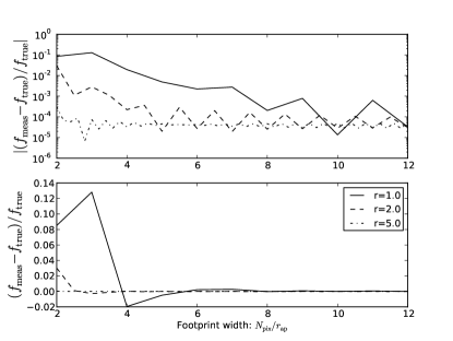
As the $w_{ij}$ coefficients are non-zero outside the aperture radius, they cannot be ignored and the footprint for the aperture (the $n_{x}\times n_{y}$ image containing the $w_{ij}$ coefficients) must be larger than the aperture itself. To determine the required footprint size, Gaussian PSFs were planted in images of varying size: $2-12\times r_{\mathrm{ap}}$. These were compared to the known values for a double Gaussian analytically integrated over the same aperture. A well-sampled double Gaussian ($\sigma_{\mathrm{core}}=1.2$ pixels) was used with aperture radii of $r_{\mathrm{ap}}$=1.0, 2.0, and 5.0 pixels. For small apertures ($<2$ pixel), errors can be as large as a few percent if the footprint is too small. For large apertures, errors are negligible even for footprints only slightly larger than the aperture radius. Empirically, we find that with a 4 pixel border around the aperture, errors are reduced to $<0.001$ for a well-sampled PSF. Figure 4 shows the flux error as a function of the width of the footprint.

Figure 4: The flux error occuring at different footprint sizes (lower panel). Absolute values are shown on a semilog scale (upper panel) to allow small values to be distinguished. The flux error for a well-sampled ($\sigma=1.2$ pixel) double-Gaussian PSF is influenced by the width of the footprint used to compute the aperture flux. The pixels outside the aperture carry weight, and the footprint must be larger than the aperture to include them. Results for three aperture radii are shown: $r$=1.0, 2.0, and 5.0. Footprint widths are normalized by the aperture radius. Footprint widths smaller than two aperture radii would explicitly exclude a portion of flux and were not considered. The error is large only when small apertures are used with small footprints. A footprint having a 4 pixel border around the aperture is sufficient to achieve $<0.001$ fractional flux error for even the smallest aperture.

3.2 The Effects of Noise

Poisson noise is always present in an astrophysical image and has a flat power spectrum which is not band limited. The sinc aperture flux $f$ can be regarded as a simple weighted sum of pixel intensities, $I_{i}$.

$$f=\sum_{i}w_{i}I_{i}$$ (7)

The variance of the sum, assuming a pixel variance $\sigma_{i}^{2}$ is

$$\sigma_{f}^{2}=\sum_{i}w_{i}^{2}\sigma_{i}^{2}.$$ (8)

Equations 7 and 8 remain true regardless of the choice of weight values, and the variances of two candidate weighting methods can be compared as a ratio. For constant pixel noise $\sigma_{I}$ (i.e. sky limited observations), the sinc aperture compared to a top hat aperture having $w_{i}=1$ gives a ratio of

$$\sigma_{f_{\mathrm{sinc}}}^{2}/\sigma_{f_{\mathrm{tophat}}}^{2}=\sum_{i}w_{i}^{2}/N.$$ (9)

The number of pixels $N$ is the area of the comparison aperture, and $\sum_{i}w_{i}^{2}$ can be regarded as a noise equivalent area (King 1983), i.e. the area of a unity-weighted aperture which would contribute the same variance to the measurement. For the sinc aperture, Figure 5 (upper panel) shows equation 9 versus aperture radius, with the denominator replaced by the area of the circular aperture being measured.

Figure 5: The noise effective area ($\sum_{i}w_{i}^{2}/\pi r^{2}$, top panel), and the signal to noise ratio (bottom panel) for circular sinc apertures as functions of aperture radius in pixels. For large apertures, the noise effective area approaches 1 and S/N approaches that of a unity-weighted ‘tophat’ aperture (shown dashed). For small radii, the noise effective area is smaller for the sinc aperture, and the S/N approaches a constant rather than zero. The S/N curve is based on a double-Gaussian PSF with $\sigma_{\mathrm{core}}$=1.5 pixel. Optimal S/N for both methods is near $\sim 1.6\sigma_{\mathrm{core}}$.

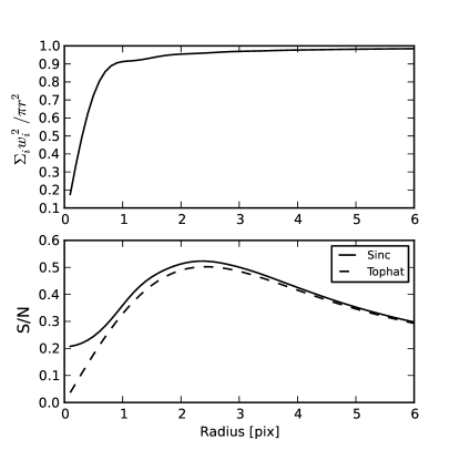
For large aperture radii, the noise equivalent area asymptotically approaches 1, but it decreases for small apertures. The noise in a sinc flux is less than would be expected in a unity-weighted ‘top hat’ aperture! The inclusion of pixels outside the aperture radius might be expected to introduce additional noise, but instead serves to reduce the overall variance. The pixels are present outside the aperture radius, but they carry less weight and the noise is averaged over a larger sample of pixels.

Note that we have not considered the shape of the PSF. We have demonstrated only that a measurement performed with a circular sinc aperture will have lower variance than one performed with a ‘top hat’ aperture. By considering the PSF, we can determine the signal to noise ratio as a function of aperture radius. This is shown for a double Gaussian with $\sigma_{\mathrm{core}}$=1.5 pixels in the lower panel of Figure 5. Curves for both sinc and top hat apertures are shown. The peak S/N at $\sim 1.6\times\sigma_{\mathrm{core}}\approx 2.4$ pixels is a known result for a Gaussian PSF (see for example Pritchet & Kline 1981). However, as the S/N deteriorates to zero for the top hat aperture, it levels off to a constant for the sinc aperture. Thus, though S/N is not optimal at small radii, it approaches a constant rather than zero.

4 Fast Computation of Coefficients

The $w_{ij}$ double integral in equation 6 can be pre-computed, but is still computationally intensive. However, by appealing to Fourier methods a fast computation algorithm is available. By expressing the aperture as a top hat function with radius $\rho$, $\Pi((x^{2}+y^{2})^{1/2}/2\rho)$, and noting that the $\mathrm{sinc}$ functions are even (i.e., $\mathrm{sinc}(\pi(x-x_{i}))=\mathrm{sinc}(\pi(x_{i}-x))$), the integral can be expressed as the convolution of a two-dimensional Cartesian $\mathrm{sinc}$ with a circular top hat, sampled discretely at $x_{i},y_{j}$:

$$w_{ij}=\iint\limits\ \Pi(x,y)\ \frac{\sin(\pi(x_{i}-x))}{\pi(x_{i}-x)}\ \frac{\sin(\pi(y_{j}-y))}{\pi(y_{j}-y)}\ \mathrm{d}x\ \mathrm{d}y.$$ (10)

The convolution can be computed quickly as a product of the Fourier-transformed functions in the wave-number domain. Both functions have analytic transforms:

$$\Pi\left(\frac{(x^{2}+y^{2})^{\frac{1}{2}}}{2\rho}\right)\Leftrightarrow\frac{\rho\ \mathrm{J}_{1}\left(2\pi\rho(k_{x}^{2}+k_{y}^{2})^{\frac{1}{2}}\right)}{(k_{x}^{2}+k_{y}^{2})^{\frac{1}{2}}},$$ (11)

and

$$\mathrm{sinc}\left(\pi(x_{i}-x)\right)\mathrm{sinc}\left(\pi(y_{i}-y)\right)\Leftrightarrow\Pi\left(\frac{k_{x}}{\pi}\right)\Pi\left(\frac{k_{y}}{\pi}\right).$$ (12)

The former yields an Airy function, and the latter yields a two-dimensional boxcar that extends to the Nyquist wave numbers. The coefficients can be obtained by computing the product of the wave-number domain components from equations 11 and 12, and taking the inverse Fourier transform:

$$w=\mathcal{F}^{-1}\left\{\Pi\left(\frac{k_{x}}{\pi}\right)\Pi\left(\frac{k_{y}}{\pi}\right)\frac{\rho\ \mathrm{J}_{1}\left(2\pi\rho(k_{x}^{2}+k_{y}^{2})^{\frac{1}{2}}\right)}{(k_{x}^{2}+k_{y}^{2})^{\frac{1}{2}}}.\right\}$$ (13)

This can be computed with a fast Fourier transform (FFT). The array of values in the wave-number domain extends out to the Nyquist wave number – precisely where the boxcar truncates the Airy function. Thus, instead of performing the real-space integral in equation 6, the $w_{ij}$ coefficients can be found directly by computing the values for the Airy function (equation 11), and taking the inverse FFT. The transformed $w_{ij}$ coefficients are entirely real-valued, and the coefficients are mathematically identical to those shown in Figure 3.

Benchmark calculations of the $w_{ij}$ coefficients for apertures with radii $r=1-10$ pixels found $\sim 10000\times$ speed increases ($\lesssim 1$ ms versus several seconds) when calculations were performed in the wave-number domain.

4.1 Shifting the Aperture Centroid

The centroid of a PSF is typically measured with sub-pixel accuracy, and it is essential that it be possible to recenter our aperture on non-integer pixel coordinates. If the $w_{ij}$ coefficients are pre-computed for integer pixel coordinates, $\mathrm{sinc}$-interpolation can be used to shift them by the necessary sub-pixel offset, $\delta_{x},\delta_{y}$.

As previously discussed, $\mathrm{sinc}$-interpolation is valid only for functions that are band limited. We demonstrated that a PSF can be treated as a band-limited function, but have not done so for the $w_{ij}$ components. However, the $w_{ij}$ components represent the aperture convolved with a $\mathrm{sinc}$ function. As a $\mathrm{sinc}$ function is itself band limited, it follows by the convolution theorem, that any convolution with it will also form a band-limited function. The $w_{ij}$ coefficients can safely be shifted by $\mathrm{sinc}$-interpolation.

It is also possible to apply a sub-pixel shift directly to $w_{ij}$ coefficients when they are created with the FFT method. To perform aperture photometry on several sources, shifting pre-computed $w_{ij}$ coefficients is faster than directly computing them for each source individually, but only slightly. If this approach is taken, shifting can be achieved easily in the wave-number domain by applying the Shift Theorem ($f(x-\delta)\Leftrightarrow e^{-i2\pi\delta k}F(k)$). Dropping the redundant $\Pi(k/\pi)$ terms, equation 13 then becomes

$$w=\mathcal{F}^{-1}\left\{e^{-i2\pi(\delta_{x}k_{x}+\delta_{y}k_{y})}\ \frac{\rho\ \mathrm{J}_{1}\left(2\pi\rho(k_{x}^{2}+k_{y}^{2})^{\frac{1}{2}}\right)}{(k_{x}^{2}+k_{y}^{2})^{\frac{1}{2}}}\right\}.$$ (14)

Due to the shift, the wave-number domain components are neither real-valued nor even. However, the application of the shift term, $e^{-i2\pi\delta k}$, preserves conjugate symmetry (i.e., if $f(x)$ is real-valued, then $F(k)=F^{*}(-k)$, where ‘^∗’ denotes complex conjugation). With conjugate symmetry, the spatial domain values (i.e., in pixel space) are guaranteed to be real-valued. This is not surprising given the physical interpretation of a shift in the spatial domain.

5 Other Apertures

Photometry with any aperture can be performed with this method; the circular aperture is conventional in observational astronomy, and conveniently has an analytic form in the wave-number domain. If the Fourier transform of the desired aperture can be accurately computed, it can be substituted for the Airy function in equations 13 and 14.

If the desired aperture has no analytic transform, the $\mathrm{sinc}$ convolution integral in equation 6 can be computed directly. As this is more computationally intensive, it could be impractical to recompute for each source being measured, and the integral should be pre-computed and shifted to the pixel coordinates of the object being measured.

5.1 Annular Apertures

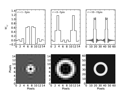
Due to the addition theorem ($f(x)+g(x)\Leftrightarrow F(k)+G(k)$), an annular aperture can be constructed trivially by taking a difference of Airy terms representing the inner and outer radii of the annulus. The $w_{ij}$ coefficients for a range of annular apertures are shown in Figure 6.

Figure 6: The $w_{ij}$ coefficients shown as images (bottom), and cross-sections through the middle row (top) for annular apertures with inner/outer radii $r=1-2$ pix (left), $r=3-5$ pix (middle), and $r=10-15$ pix (right).

5.2 Elliptical Apertures

The special case of an elliptical aperture can be handled by applying the Similarity Theorem ($f(ax)\Leftrightarrow|a|^{-1}F(k/a)$) to the circular case. The compression of a circle along a given axis forms an ellipse, and the corresponding Fourier transform can be formed by dilating that of a circle along the appropriate axis.

The Fourier transform preserves rotation; if $f(x,y)$ is rotated by $\theta$ degrees, $F(k_{x},k_{y})$ will be rotated by a corresponding amount in the same sense. We therefore compress the Airy function along the $k_{y}$ axis, and rotate it by the desired amount with a rotation matrix applied to the $k_{x},k_{y}$ wave numbers.

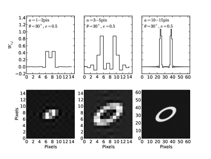
To demonstrate all the properties presented, $w_{ij}$ coefficients for a selection of annular elliptical apertures are shown in Figure 7.

Figure 7: The $w_{ij}$ coefficients shown as images (bottom), and cross-sections through the middle row (top) for annular elliptical apertures with inner/outer semi-major axes $a=1-2$ pix (left), $a=3-5$ pix (middle), and $a=10-15$ pix (right). Ellipses are rotated by $\theta=30^{\circ}$ and have ellipticity $e=1-b/a=0.5$, where $b$ and $a$ are the semi-minor and semi-major axes, respectively.

In Appendix B, we include a sample of Python code that demonstrates the method by computing growth curves for model PSFs. The coefficient images in Figures 3, 6, and 7 were constructed with the wijCoefficients() routine included in the sample code.

6 Performance and Effectiveness of the Algorithm

The accuracy of the method was tested by constructing and measuring images of sources with known PSFs and fluxes. Two different tests were performed. In the first test, aperture magnitudes were measured for progressively larger apertures to determine the growth curves for model PSFs, and these were compared to those of the known, analytic solutions. In addition to the double Gaussian PSF used throughout this work, the popular Moffat PSF (Moffat 1969) was also tested. In the second test, our aperture magnitudes were compared to values produced by the SExtractor software package (Bertin & Arnouts 1996).

6.1 Measuring the Growth Curves for Double Gaussian and Moffat PSFs

For simplicity, analytic double Gaussian and Moffat PSFs were used for testing. Neither is a band-limited function, and different widths ($\sigma_{\mathrm{core}}$ values for the double Gaussians and FWHM for the Moffat PSFs) were tested to evaluate the behaviour near the critical sampling limit, $\sigma_{\mathrm{core}}=1$ pixel. The pixel values for the double Gaussian were computed at coordinates $x,y$ with

$$p_{ij}=\frac{1}{2\pi\left(\sigma^{2}_{\mathrm{core}}+b\sigma^{2}_{\mathrm{wing}}\right)}\left[e^{\frac{-(x^{2}+y^{2})}{2\sigma_{\mathrm{core}}^{2}}}+b\ e^{\frac{-(x^{2}+y^{2})}{2\sigma_{\mathrm{wing}}^{2}}}\right].$$ (15)

Here, $\sigma_{\mathrm{wing}}=2\sigma_{\mathrm{core}}$, and $b=0.1$. Values for the Moffat PSF were computed with

$$p_{ij}=\frac{\beta-1}{\pi\alpha^{2}}\left[1.0+\frac{x^{2}+y^{2}}{\alpha^{2}}\right]^{-\beta}$$ (16)

where $\beta=4.765$ (Trujillo et al. 2001), and $\alpha=\mathrm{FWHM}/2(2^{1/\beta}-1)^{1/2}$. The FWHM used to compute the Moffat PSF was $2.4670\sigma_{\mathrm{core}}$. Note that this differs slightly from the value of FWHM=$2.3548\sigma$ for a single Gaussian.

Note that these are a sampling of the PSFs as we do not integrate over the pixels. The PSF is considered to be a combination of multiple contributing components, including the aperture response (an Airy function), the atmospheric blurring, and the pixel response.

Three widths were evaluated: $\sigma_{\mathrm{core}}$=0.8, 1.0, and 1.2 pixels, corresponding to under-, critical-, and well-sampled PSFs. Sources were planted in the center of a 16$\times$16 pixel image. Additional sub-pixel offsets were applied to test the effects of shifting the aperture.

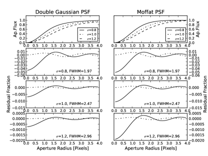
Sinc-integrated aperture fluxes were measured from the images with aperture radii, $0<r<4$ pixels (0.1 pixel increments). The known PSFs (equation 15) were then integrated directly over the same apertures to obtain the true theoretical fluxes. The structure of the residuals varies depending on the sub-pixel shift applied. For both PSFs, the smallest residual was observed when no sub-pixel offset was applied, and the largest residual was observed when half-pixel offsets were applied to both $x$ and $y$. Discrepancies are highest for apertures with radii $<1$ pixel. Growth curves of the measured fluxes are presented with residuals in Figure 8. To illustrate the effects of the sub-pixel shift, the curves shown are those representing the extrema.

The amplitudes of the residual curves decrease rapidly as sampling improves. Discrepancies as high as a few percent can be seen for the undersampled PSFs, and the method is clearly unsuitable under such conditions. The well-sampled PSF ($\sigma_{\mathrm{core}}=1.2$, FWHM$=3.0$) performs extremely well at all aperture sizes (fractional residual less than $0.001$ and $0.002$ for double Gaussian and Moffat, respectively).

Figure 8: Measured growth curves and residuals with respect to computed theoretical fluxes. Left and right panels show values for double-Gaussian and Moffat PSFs, respectively. PSF widths of $\sigma$=0.8, 1.0, and 1.2 pixels were used to evaluate under-, critical-, and over-sampling. The differences between the measured and theoretical curves are too small to be seen directly, but are shown as residuals in the three lower panels. Residuals shown with a dashed line are the minimum observed, and correspond to no sub-pixel shift. Those shown with a solid line are the maxima, and correspond to a half-pixel shift in both $x$ and $y$ coordinates. The curves are very similar in structure, but differ dramatically in amplitude. The method is clearly unsuitable for sub-sampled ($\sigma<1.0$ pixel) PSFs, but performs extremely well for $\sigma\gtrsim 1.2$ pixel.

6.2 Comparison to SExtractor Aperture Magnitudes

We also compared sinc magnitudes to the values produced by the SExtractor software package (Bertin & Arnouts 1996) version 2.3.2. SExtractor is one of the most widely used photometry packages in the astronomy community and is the most suitable algorithm for such a comparison.

Double Gaussian PSFs were added to the center of $24\times 24$ pixel images. Tests were performed with well-sampled ($\sigma_{\mathrm{core}}$=1.5 pixel) and under-sampled ($\sigma_{\mathrm{core}}$=0.7 pixel) double Gaussians. As with previous tests, the wing component was 2$\times$ wider and had an amplitude which was 10$\%$ of the core component’s amplitude. Each test was run with and without noise for aperture radii of $r$=1.0, 2.0, and 5.0 pixels. The tests performed with noise included a 100 count sky level, and the pixel values were replaced with random Poisson variates. For simplicity, a gain of 1.0 was used.

For a given test, 500 trials were run for fluxes covering several magnitudes. In each case, the double Gaussian was given a random sub-pixel offset. The test image was written to a FITS file and was measured with both SExtractor and the sinc algorithm. In order to ensure that only the photometric algorithms were compared, the sinc algorithm was run using the $x,y$ pixel centroids as measured by SExtractor. The PHOT_APERTURES parameter was set to 2$\times$ the radius (SExtractor specifies aperture diameter), and MAG_ZEROPOINT was set to an arbitrary value of 25. For tests including noise and sky, the known sky level of 100 counts was subtracted before processing, and SExtractor’s BACK_TYPE parameter was set to MANUAL to disable internal background estimation. Results of the testing are shown in Figures 9 (well-sampled PSF), and 10 (under-sampled PSF).

Figure 9: Magnitude error versus known magnitude for sinc (dots) and SExtractor ($+$ symbols) aperture magnitudes of well-sampled PSFs. A lower sub-plot shows the standard deviation of points in bins with width 0.5 mag. Well-sampled double-Gaussian PSFs ($\sigma_{\mathrm{core}}$=1.5 pixel) were added to $24\times 24$ pixel images and were measured with both algorithms. Aperture radii of $r$=1.0 (top), 2.0 (middle), and 5.0 (lower) pixels were used. Left panels show results for which no noise was added to the double-Gaussian PSFs, and right panels show results which included Poisson noise and the addition of a 100 count sky level. For apertures with $r\gtrsim$5.0 pixels, performance is similar for both algorithms. For smaller apertures, the sinc method outperforms in both precision and accuracy.

Figure 10: Magnitude error versus known magnitude for sinc (dots) and SExtractor ($+$ symbols) aperture magnitudes of under-sampled PSFs. The panels are the same as those described in Figure 9. In this case, under-sampled (0.7 pixel) double-Gaussian PSFs were used. For large apertures the SExtractor magnitudes are more precise and more accurate than the sinc magnitudes. For small apertures, the sinc magnitudes are more precise and more accurate, becoming the better option for apertures with $r\lesssim$1.0 pixel.

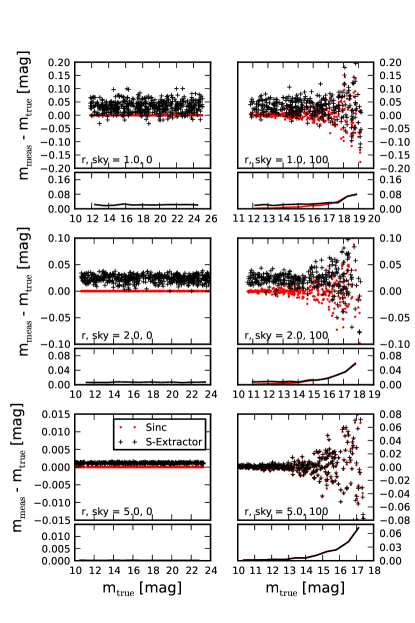
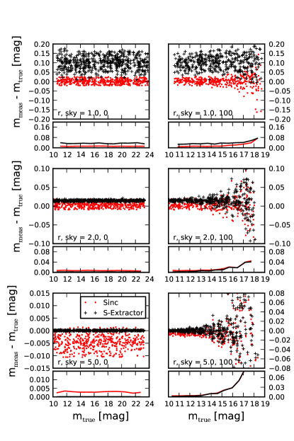
For well-sampled data measured with a large ($r\gtrsim$5 pixel) aperture, the performance of the two algorithms is similar. For smaller apertures, the sinc algorithm outperforms SExtractor. In the case of under-sampled data with a large aperture, SExtractor outperforms. However, this performance deteriorates for smaller apertures while the sinc algorithm’s does not. For $r\lesssim$1.0 pixel apertures, the sinc method yields the better result.

7 Discussion

The method we have described relies on very well-established mathematical theorems, namely the sampling theorem, and various theorems associated with the Fourier transform. However, various aspects of our analysis require some discussion.

Our decision to use pure sinc interpolation in place of a Lanczos kernel (a tapered sinc function, see Lanczos (1956)) requires some justification. When we integrate the sinc function over the aperture, it is defined within the entire region of integration, regardless of the location of the sinc peak (i.e. the pixel in $w_{ij}$ being considered). The value obtained for each $w_{ij}$ pixel is therefore more accurate than that which would be obtained by a Lanczos, which tapers to zero beyond its region of support (typically 4 to 7 pixels). However, this difference is truly negligible. Our principal reason for using a pure sinc was that it offers a convenient Fourier transform (unity throughout our region of interest in the wave-number domain). In order to minimize demand on computing resources for e.g. a Kron flux, computation in the wave-number domain is essential. The Fourier transform of a Lanczos kernel is sufficiently complicated that the pure sinc is the better choice.

As there are a variety of PSF models available, an alternative to measuring aperture fluxes directly would be to fit an appropriate model and integrate the model over the desired aperture. When the object being measured is not a point source, this approach is often preferred. In such cases, the objects have different sizes and shapes, and use of a constant aperture radius would not allow objects to be meaningfully compared. Model fluxes can frequently be the best choice in such situations. However, for the purpose of calibration, the use of a model introduces an unnecessary source of potential systematic error. A poorly chosen model will never fit properly and will corrupt the aperture correction and thus the zero point of the calibration.

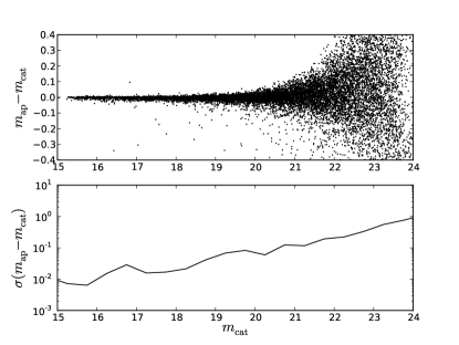
As a more practical verification of the method, the sinc-interpolated aperture fluxes are being used to compute aperture fluxes, and to determine the aperture correction for the LSST photometric pipeline that is currently under development. The sinc method has been found to perform extremely well, providing $\left<m_{\mathrm{PSF}}-m_{\mathrm{ap}}\right>\lesssim 0.001$ (verifying aperture correction), and $\left<m_{\mathrm{ap}}-m_{\mathrm{cat}}\right>\lesssim 0.001$ (verifying measurement accuracy). Here, $m_{\mathrm{PSF}}$ and $m_{\mathrm{ap}}$ are PSF and (sinc) aperture magnitudes, and $m_{\mathrm{cat}}$ is a catalog magnitude corresponding to the known input flux in a simulated image. Several hundred simulated images have been generated, processed, and tested, covering a variety of observing conditions (cloud, seeing, etc). The LSST simulator uses a ray-tracing algorithm to trace photons through a simulated atmosphere and through simulated optics to produce each test image (Peterson et al. 2013, in preparation). The ray-tracing simulations include realistic field-dependent and wavelength-dependent effects that result in complex point-spread functions and photometric variation that challenge photometry algorithms. . The aperture magnitudes show no systematic trends with magnitude, and the variability in shape and PSF width observed across a focal plane of individual CCD images is handled well by a 2D polynomial aperture correction. An example of sinc aperture photometry performed on LSST simulated data is shown in Figure 11. As yet, no failure modes have been observed for the algorithm.

Figure 11: Sinc aperture photometry performed on a simulated LSST $i^{\prime}$ image (Peterson et al. 2013, in preparation). For clarity, only 1/4 of the values from a full frame are shown. The upper panel shows $m_{\mathrm{ap}}-m_{\mathrm{cat}}$ versus $m_{\mathrm{cat}}$, and the lower panel shows the standard deviation of the upper panel data in 0.5 mag bins. The aperture radius was 7 pixels (1.4″), and magnitudes are compared to the exact known values (i.e. $m_{\mathrm{cat}}$) used as input for the simulator.

As stated earlier, any error introduced as a result of a non-band-limited PSF will not be systematic. Even if a constant radius aperture is used for aperture photometry, the error will depend on the sub-pixel shift of the PSF and will thus be different for each measured source. Adequate sampling is essential, but we believe our tested limit of $\sigma>1.2$ pixels (FWHM $>3.0$ pixels) is a reliable benchmark.

8 Summary

We have developed an algorithm for performing aperture photometry on critically sampled astrophysical images. The flux is numerically integrated over the desired aperture, with sinc-interpolation used to reconstruct values between pixels. As the pixel values can be factored out of the computationally intensive integral, only the $\mathrm{sinc}$ functions need to be integrated, and these can be pre-computed and applied to an arbitrary number of aperture flux measurements.

The aperture flux is ultimately computed as a weighted sum of pixel values, with the sinc-integrals providing the weights. The weight values are non-zero outside the nominal cut-off radius of the aperture. We find that an aperture flux must be measured in a footprint with a border extending $\sim$4 pixels beyond the aperture limits to ensure accuracy.

Using Fourier methods, we have shown that the integral of the sinc-functions over the aperture is a convolution integral, and can be computed quickly as a product in the wave-number domain.

As the method relies on sinc-interpolation based on the sampling-theorem, a band-limited PSF is an implicit assumption. A rule of thumb for this requirement to be satisfied is that a double-Gaussian PSF must be sampled such that $\sigma>1.2$ pixels, or equivalently FWHM $>3.0$ pixels. No Gaussian-based function is truly band limited, but this rule of thumb reduces the photometric error contributed by the aperture to $<0.001$ mag. If the requirement is not satisfied, the resulting error depends on the sub-pixel position of the PSF and cannot be corrected during calibration. The error is also a function of aperture radius, and the band-limited requirement must be satisfied to produce an accurate growth curve.

Comparison with SExtractor demonstrated that the sinc method provides equal performance for large apertures ($r\gtrsim$5 pixel), and much better performance for smaller apertures. However, for under-sampled data, the best results were obtained with SExtractor using a large aperture.

The method performs equally well for annular and elliptical apertures, and can be adapted for any aperture. To demonstrate the method, a short example has been coded in Python and is presented in Appendix B.

In closing, we note that the Sloan Digital Sky Survey’s photometric pipeline used a version of this technique for the measurement of aperture fluxes. In that version, the $w_{ij}$ components (see equation 10) were pre-computed as real-space 2D integrals prior to frame processing, and were Lanczos-shifted to be recentred on each source for flux measurement. As the SDSS photometric catalog is among the most widely used data sets in the astronomy community, the effectiveness of the algorithm has been very well demonstrated in practice. The method is now being used in the LSST photometric pipeline under development, with the only difference being the use of Fourier methods to more efficiently generate the $w_{ij}$ components. Tests on simulated LSST images have shown the algorithm to perform efficiently (i.e., quickly) and produce Poisson-limited accuracy.

Appendix A The Fractional Aliased Power in a Sampled Gaussian

The principal requirement for the sinc reconstruction to be valid is that the PSF be band-limited. To test this assumption analytically, we approximate the PSF, $p(r)$, as a circular bivariate Gaussian, which has a convenient analytic Hankel transform $P(q)$ (circularly symmetric form of the Fourier transform):

$$p(r)=e^{-r^{2}/2\sigma^{2}}\Leftrightarrow P(q)=\sigma^{2}e^{-q^{2}\sigma^{2}/2},$$ (17)

where $\Leftrightarrow$ denotes a transform pair.

The aliased power beyond the band-limit for a Gaussian ($>\pi$ when $\sigma$ is in pixel units) is

$$\mathrm{aliased\ power}=2\pi\int_{\pi}^{\infty}\sigma^{4}e^{-q^{2}\sigma^{2}}\ q\ \mathrm{d}q=\pi\sigma^{2}e^{-\pi^{2}\sigma^{2}},$$ (18)

where the integrand is the power from equation 17. Under the assumption that the pixels are square, the convenient circular symmetry used here is an approximation, but a very good one. The Fourier transform of a real PSF should be integrated in two dimensions with limits $k_{x,y}<-\pi,k_{x,y}>\pi$, so our use of circular symmetry ($q=(k_{x}^{2}+k_{y}^{2})^{1/2}>\pi$) is conservative in that it omits power that is not actually lost in Cartesian coordinates (i.e., the corners of the region in the wave-number domain where $\pi<(k_{x}^{2}+k_{y}^{2})^{1/2}$).

Next, we translate the aliased power to a corresponding error in flux using Rayleigh’s Theorem applied to the Hankel transform:

$$\int_{0}^{\infty}|p(r)|^{2}\ r\ \mathrm{d}r=\int_{0}^{\infty}|P(q)|^{2}\ q\ \mathrm{d}q.$$ (19)

The aliased power equals the integral of the squared error $|\epsilon(r)|^{2}$, which that power represents in the spatial domain. By taking the square root, we obtain a flux error estimate :

$$\mathrm{error} = \left(2\pi\int_{0}^{\infty}|\epsilon(r)|^{2}\ r\ \mathrm{d}r\right)^{1/2}$$ (20)

$$= \left(2\pi\int_{\pi}^{\infty}\sigma^{4}e^{-q^{2}\sigma^{2}}q\ \mathrm{d}q\right)^{1/2}$$ (21)

$$= \pi^{1/2}\sigma e^{-\pi^{2}\sigma^{2}/2}.$$ (22)

The total integrated flux is $2\pi\sigma^{2}$, and the error shown as a fraction is

$$\frac{\mathrm{error}}{\mathrm{total\ flux}}=\frac{e^{-\pi^{2}\sigma^{2}/2}}{2\pi^{1/2}\sigma}.$$ (23)

Equation 23 can be used as an estimate of the systematic flux error introduced by aliased power. Three assumptions were implicitly made to simplify the estimate: (1) circular symmetry can be used as an approximation in equation 18, (2) the power above the Nyquist wave number is simply lost rather than being aliased back into the pass band, and (3) the flux being integrated is the total flux integrated to infinity rather than that within a limited aperture radius. All of these assumptions tend to overestimate the error, and equation 23 can be regarded as providing an upper limit on the systematic flux error.

Appendix B Sample Code to Demonstrate Sinc Aperture Photometry

The following sample of Python code demonstrates the sinc method for performing aperture photometry. Python is an open-source scripting language, and is readily available on most computing platforms (see http://www.python.org). Our example uses the numpy and scipy modules (available at http://numpy.scipy.org/ and http://www.scipy.org/, respectively).

Due to the nature of Python, the indentation structure is essential. The authors will gladly provide a digital copy upon request. Note that the code is intended only as an example, and is not written with efficiency in mind. Computing performance can be greatly improved by transcribing the code to C, C++, or some other compiled language. A C++ version of the algorithm is included in the LSST code stack. For information on downloading the LSST source code see www.lsst.org).

The following command will run the example (assuming the script has been named sinc_phot.py), which will plant a Gaussian PSF with $\sigma=1.2$ centred at $x,y=16,16$ in a $n=32\times 32$ pixel image, and will compute a growth curve for it with the sinc-aperture method. Output is printed to the screen (i.e., stdout).

./sinc_phot.py 32 16.0 16.0 1.2
(i.e., ./sinc_phot.py n x y $\sigma$)

The function wijCoefficients() is capable of computing annular and/or elliptical aperture coefficients, but values for the ellipticity, position angle (theta), and inner radius are set to 0.0 in the example.

#!/usr/bin/env python
import sys, numpy, scipy.special as special

def gaussianImage(n, center_x, center_y, sigma):
    image = numpy.zeros([n, n], dtype=float)
    for ix in range(n):
        for iy in range(n):
            x, y = ix - center_x, iy - center_y
            A = 1.0/(2.0*numpy.pi*sigma**2)
            image[iy,ix] = A*numpy.exp(-(x**2 + y**2)/(2.0*sigma**2))
    return image

def wijCoefficients(n, x, y, rad1, rad2, theta, ellipticity):
    wid, xcen, ycen = n, (n+1)/2, (n+1)/2
    dx, dy = x - xcen, y - ycen
    if n%2:
        dx, dy = dx + 1, dy + 1

    ftWij = numpy.zeros([wid, wid], dtype=complex)
    scale     = 1.0 - ellipticity
    for iy in range(wid):
        ky = float(iy - ycen)/wid
        for ix in range(wid):
            kx = float(ix - xcen)/wid

            # rotate and rescale
            cosT, sinT = numpy.cos(theta), numpy.sin(theta)
            kxr, kyr =  kx*cosT + ky*sinT, scale*(-kx*sinT + ky*cosT)
            k = numpy.sqrt(kxr**2 + kyr**2)

            # compute the airy terms, and apply shift theorem
            if k != 0.0:
                airy1 = rad1*special.j1(2.0*numpy.pi*rad1*k)/k
                airy2 = rad2*special.j1(2.0*numpy.pi*rad2*k)/k
            else:
                airy1, airy2 = numpy.pi*rad1**2, numpy.pi*rad2**2
            airy = airy2 - airy1
            phase = numpy.exp(-1.0j*2.0*numpy.pi*(dx*kxr + dy*kyr))

            ftWij[iy,ix] = phase*scale*airy

    ftWijShift = numpy.fft.fftshift(ftWij)
    wijShift   = numpy.fft.ifft2(ftWijShift)
    wij        = numpy.fft.fftshift(wijShift)
    return wij.real

if __name__ == ’__main__’:
    n = int(sys.argv[1])
    x, y, psf_sigma = map(float, sys.argv[2:])
    radius_inner, theta, ellipticity = 0.0, numpy.pi*(0.0)/180.0, 0.0

    psf = gaussianImage(n, x, y, psf_sigma)
    for radius in numpy.arange(radius_inner + 0.1, 6.0*psf_sigma, 0.1):
        wij = wijCoefficients(n, x, y, radius_inner, radius, theta, ellipticity)
        flux_measured = (psf*wij).sum()
        flux_analytic = (1.0 - numpy.exp(-radius**2/(2.0*psf_sigma**2)))
        print radius, flux_measured, flux_analytic

References

- Bertin & Arnouts (1996) Bertin E., Arnouts S., 1996, A&AS, 117, 393
- Ivezic et al. (2008) Ivezic Z., Tyson J. A., Acosta E., et al., 2008, ArXiv e-prints
- King (1983) King I. R., 1983, PASP, 95, 163
- Kron (1980) Kron R. G., 1980, ApJS, 43, 305
- Lanczos (1956) Lanczos C., 1956, Applied Analysis. Englewood Cliffs, NJ: Prentice-Hall
- Moffat (1969) Moffat A. F. J., 1969, A&A, 3, 455
- Peterson et al. (2013) Peterson J., et al., 2013, Simulation of Astronomical Images from Optical Survey Telescopes using Comprehensive Monte Carlo Approach, In preparation
- Petrosian (1976) Petrosian V., 1976, ApJ, 209, L1
- Pritchet & Kline (1981) Pritchet C., Kline M. I., 1981, AJ, 86, 1859
- Shannon (1949) Shannon C. E., 1949, Proc. IRE, 37
- Stetson (1987) Stetson P. B., 1987, PASP, 99, 191
- Tody (1986) Tody D., 1986, in Crawford D. L., ed., Society of Photo-Optical Instrumentation Engineers (SPIE) Conference Series Vol. 627 of Society of Photo-Optical Instrumentation Engineers (SPIE) Conference Series, The IRAF Data Reduction and Analysis System. pp 733–+
- Trujillo et al. (2001) Trujillo I., Aguerri J. A. L., Cepa J., Gutiérrez C. M., 2001, MNRAS, 328, 977