Contemporaneous aggregation of triangular array
of random-coefficient AR(1) processes

Abstract

We discuss contemporaneous aggregation of independent copies of a triangular array of random-coefficient AR(1) processes with i.i.d. innovations belonging to the domain of attraction of an infinitely divisible law $W$. The limiting aggregated process is shown to exist, under general assumptions on $W$ and the mixing distribution, and is represented as a mixed infinitely divisible moving-average $\{\mathfrak{X}(t)\}$ in (1.4). Partial sums process of $\{\mathfrak{X}(t)\}$ is discussed under the assumption $\mathrm{E}W^{2}<\infty$ and a mixing density regularly varying at the “unit root” $x=1$ with exponent $\beta>0$. We show that the above partial sums process may exhibit four different limit behaviors depending on $\beta$ and the Lévy triplet of $W$. Finally, we study the disaggregation problem for $\{\mathfrak{X}(t)\}$ in spirit of Leipus et al. (2006) and obtain the weak consistency of the corresponding estimator of $\phi(x)$ in a suitable $L_{2}-$space.

Keywords: Aggregation; random-coefficient AR(1) process; triangular array; infinitely divisible distribution; partial sums process; long memory; disaggregation

1 Introduction

The present paper discusses contemporaneous aggregation of $N$ independent copies

$$X^{(N)}_{i}(t)=a_{i}X^{(N)}_{i}(t-1)+\varepsilon^{(N)}_{i}(t),\qquad t\in\mathbb{Z},\quad i=1,2,\cdots,N$$ (1.1)

of random-coefficient AR(1) process $X^{(N)}(t)=aX^{(N)}(t-1)+\varepsilon^{(N)}(t),\ t\in\mathbb{Z}$, where $\{\varepsilon^{(N)}(t),\,t\in\mathbb{Z}\},\,N=1,2,\cdots$ is a triangular array of i.i.d. random variables in the domain of attraction of an infinitely divisible law $W$:

$$\sum_{t=1}^{N}\varepsilon^{(N)}(t) \to_{\rm d} W$$ (1.2)

and where $a$ is a r.v., independent of $\{\varepsilon^{(N)}(t),t\in\mathbb{Z}\}$ and satisfying $|a|<1$ almost surely (a.s.). The limit aggregated process $\{\mathfrak{X}(t),t\in\mathbb{Z}\}$ is defined as the limit in distribution:

$$\sum_{i=1}^{N}X^{(N)}_{i}(t)\ \to_{\rm fdd}\ \mathfrak{X}(t).$$ (1.3)

Here and below, $\to_{\rm d}$ and $\to_{\rm fdd}$ denote the weak convergence of distributions and finite-dimensional distributions, respectively. A particular case of (1.1)-(1.3) corresponding to $\varepsilon^{(N)}(t)=N^{-1/2}\zeta(t),$ where $\{\zeta(t),t\in\mathbb{Z}\}$ are i.i.d. r.v.’s with zero mean and finite variance, leads to the classical aggregation scheme of Robinson (1978), Granger (1980) and a Gaussian limit process $\{\mathfrak{X}(t)\}.$ See also Gonçalves and Gourièroux (1988), Zaffaroni (2004), Oppenheim and Viano (2004), Celov et al. (2007), Beran et al. (2010) on aggregation of more general time series models with finite variance. Puplinskaitė and Surgailis (2009, 2010) discussed aggregation of random-coefficient AR(1) processes with infinite variance and innovations $\varepsilon^{(N)}(t)=N^{-1/\alpha}\zeta(t),$ where $\{\zeta(t),t\in\mathbb{Z}\}$ are i.i.d. r.v.’s in the domain of attraction of $\alpha-$stable law $W,\,0<\alpha<2.$ Aggregation and disaggregation of autoregressive random fields was discussed in Lavancier (2005, 2011), Lavancier et al. (2012), Puplinskaitė and Surgailis (2012), Leonenko et al. (2013).

The present paper discusses the existence and properties of the limit process $\{\mathfrak{X}(t)\}$ in the general triangular aggregation scheme (1.1)-(1.3). Let us describe our main results. Theorem 2.6 (Sec. 2) says that under condition (1.2) and some mild additional conditions, the limit process in (1.3) exists and is written as a stochastic integral

$$\mathfrak{X}(t)\ :=\ \sum_{s\leq t}\int_{(-1,1)}x^{t-s}M_{s}({\mathrm{d}}x),\qquad t\in\mathbb{Z},$$ (1.4)

where $\{M_{s},s\in\mathbb{Z}\}$ are i.i.d. copies of an infinitely divisible (ID) random measure $M$ on $(-1,1)$ with control measure $\Phi(\mathrm{d}x):=\mathrm{P}(a\in\mathrm{d}x)$ and Lévy characteristics $(\mu,\sigma,\pi)$ the same as of r.v. $W$ ($M\sim W$) in (1.2), i.e., for any Borel set $A\subset(-1,1)$

$$\mathrm{E}\mathrm{e}^{{\mathrm{i}}\theta M(A)} = \mathrm{e}^{\Phi(A)V(\theta)},\qquad\theta\in\mathbb{R}.$$ (1.5)

Here and in the sequel, $V(\theta)$ denotes the log-characteristic function of r.v. $W$:

$$V(\theta) := \log\mathrm{E}\mathrm{e}^{\mathrm{i}\theta W}\ =\ \int_{\mathbb{R}}(\mathrm{e}^{{\mathrm{i}}\theta y}-1-{\mathrm{i}}\theta y{\bf 1}(|y|\leq 1))\pi(\mathrm{d}y)-\frac{1}{2}\theta^{2}\sigma^{2}+\mathrm{i}\theta\mu,$$ (1.6)

where $\mu\in\mathbb{R},\,\sigma\geq 0$ and $\pi$ is a Lévy measure (see sec. 2 for details). In the particular case when $W$ is $\alpha-$stable, $0<\alpha\leq 2$, Theorem 2.6 agrees with Puplinskaitė and Surgailis (2010, Thm. 2.1). We note that the process $\{\mathfrak{X}(t)\}$ in (1.4) is stationary, ergodic and has ID finite-dimensional distributions. According to the terminology in Rajput and Rosinski (1989), (1.4) is called a mixed ID moving-average.

Section 3 discusses partial sums limits and long memory properties of the aggregated process $\{\mathfrak{X}(t)\}$ in (1.4) under the assumption that the mixing distribution $\Phi$ has a probability density $\phi$ varying regularly at $x=1$ with exponent $\beta>0$:

$$\phi(x)\ \sim\ C(1-x)^{\beta},\qquad x\to 1$$ (1.7)

for some $C>0$. (1.7) is similar to the assumptions on the mixing distribution in Granger (1980), Zaffaroni (2004) and other papers. In the finite variance case $\sigma^{2}_{W}:={\rm Var}(W)<\infty$ the aggregated process in (1.4) is covariance stationary provided $\mathrm{E}(1-a^{2})^{-1}<\infty$, with covariance

$$r(t)\ :=\ {\rm Cov}(\mathfrak{X}(t),\mathfrak{X}(0))\ =\ \sigma^{2}_{W}\,\mathrm{E}\big{[}\sum_{s\leq 0}a^{t-s}a^{-s}\big{]}\ =\ \sigma^{2}_{W}\,\mathrm{E}\big{[}\frac{a^{t}}{1-a^{2}}\big{]},\quad\forall t\in\mathbb{N}$$ (1.8)

depending on $\sigma^{2}_{W}$ and the mixing distribution only. Note also that the autocorrelation function of $\mathfrak{X}$ only depends on the law of $a$. It is well-known that for $0<\beta<1$ and $a\in[0,1)$ a.s., (1.7) implies that $r(t)\sim C_{1}t^{-\beta}\,(t\to\infty)$ with some $C_{1}>0$, in other words, the aggregated process $\{\mathfrak{X}(t)\}$ has nonsummable covariances $\sum_{t\in\mathbb{Z}}|r(t)|=\infty,$ or covariance long memory.

Long memory is often characterized by the limit behavior of partial sums. According to Cox (1984), a stationary process $\{Y_{t},t\in\mathbb{Z}\}$ is said to have distributional long memory if there exist some constants $A_{n}\to\infty\ (n\to\infty)$ and $B_{n}$ and a (nontrivial) stochastic process $\{J(\tau),\tau\geq 0\}$ with dependent increments such that

$$A_{n}^{-1}\sum_{t=1}^{[n\tau]}(Y_{t}-B_{n})\ \rightarrow_{\rm fdd}\ J(\tau).$$ (1.9)

In the case when $\{J(\tau)\}$ in (1.9) has independent increments, the corresponding process $\{Y_{t},t\in\mathbb{Z}\}$ is said to have distributional short memory.

The main result of Sec. 3 is Theorem 3.1 which shows that under conditions (1.7) and $\mathrm{E}W^{2}<\infty,$ partial sums of the aggregated $\{\mathfrak{X}(t)\}$ in (1.4) may exhibit four different limit behaviors, depending on parameters $\beta,\sigma$ and the behavior of the Lévy measure $\pi$ at the origin. Write $W\sim ID_{2}(\sigma,\pi)$ if $\mathrm{E}W=0,\,\mathrm{E}W^{2}=\sigma^{2}+\int_{\mathbb{R}}x^{2}\pi(\mathrm{d}x)<\infty,$ in which case $V(\theta)$ of (1.6) can be written as

$$V(\theta) = \int_{\mathbb{R}}(\mathrm{e}^{{\mathrm{i}}\theta y}-1-{\mathrm{i}}\theta y)\pi(\mathrm{d}y)-\frac{1}{2}\theta^{2}\sigma^{2}.$$ (1.10)

The Lévy measure $\pi$ is completely determined by two nonincreasing functions $\Pi^{+}(x):=\pi(\{u>x\}),\,\Pi^{-}(x):=\pi(\{u\leq-x\}),\,x>0$ on $\mathbb{R}_{+}=(0,\infty)$. Assume that there exist $\alpha>0$ and $c^{\pm}\geq 0,c^{+}+c^{-}>0$ such that

$$\lim_{x\to 0}x^{\alpha}\Pi^{+}(x)=c^{+},\qquad\lim_{x\to 0}x^{\alpha}\Pi^{-}(x)=c^{-}.$$ (1.11)

Under these assumptions, the four limit behaviors of $S_{n}(\tau):=\sum_{t=1}^{[n\tau]}\mathfrak{X}(t)$ correspond to the following parameter regions:

(i)

$0<\beta<1,\ \sigma>0,$

(ii)

$0<\beta<1,\ \sigma=0,\ 1+\beta<\alpha<2,$

(iii)

$0<\beta<1,\ \sigma=0,\ 0<\alpha<1+\beta,$

(iv)

$\beta>1.$

According to Theorem 3.1, the limit process of $\{S_{n}(\tau)\}$, in the sense of (1.9) with $B_{n}=0$ and suitably growing $A_{n}$ in respective cases (i) - (iv) is a

(i)

fractional Brownian motion with parameter $H=1-(\beta/2),$

(ii)

$\alpha-$stable self-similar process $\Lambda_{\alpha,\beta}$ with dependent increments and self-similarity parameter $H=1-(\beta/\alpha),$ defined in (3.2) below,

(iii)

$(1+\beta)-$stable Lévy process with independent increments,

(iv)

Brownian motion.

See Theorem 3.1 for precise formulations. Accordingly, the process $\{\mathfrak{X}(t)\}$ in (1.4) has distributional long memory in cases (i) and (ii) and distributional short memory in case (iii). At the same time, $\{\mathfrak{X}(t)\}$ has covariance long memory in all three cases (i)-(iii). Case (iv) corresponds to distributional and covariance short memory. As $\alpha$ increases from $0$ to $2$, the Lévy measure in (1.11) increases its “mass” near the origin, the limiting case $\alpha=2$ corresponding to $\sigma>0$ or a positive “mass” at $0$. We see from (i)-(ii) that distributional long memory is related to $\alpha$ being large enough, or small jumps of the random measure $M$ having sufficient high intensity. Note that the critical exponent $\alpha=1+\beta$ separating the long and short memory “regimes” in (ii) and (iii) decreases with $\beta,$ which is quite natural since smaller $\beta$ means the mixing distribution putting more weight near the unit root $a=1$.

Since aggregation leads to a natural loss of information about aggregated “micro” series, an important statistical problem arises to recover the lost information from the observed sample of the aggregated process. In the context of the AR(1) aggregation scheme (1.1)-(1.3) this leads to the so-called the disaggregation problem, or reconstruction of the mixing density $\phi(x)$ from observed sample $\mathfrak{X}(1),\cdots,\mathfrak{X}(n)$ of the aggregated process in (1.4). For Gaussian process (1.4), the disaggregation problem was investigated in Leipus et al. (2006) and Celov et al. (2010), who constructed an estimator of the mixing density based on its expansion in an orthogonal polynomial basis. In Sec. 4 we extend the results in Leipus et al. (2006) to the case when the aggregated process is a mixed ID moving-average of (1.4) with finite 4th moment and obtain the weak consistency of the mixture density estimator in a suitable $L_{2}-$space (Theorem 4.1).

The results of our paper could be developed in several directions. We expect that Theorem 3.1 can be extended to the aggregation scheme with common innovations and to infinite variance ID moving-averages of (1.4), generalizing the results in Puplinskaitė and Surgailis (2009, 2010). An interesting open problem is generalizing Theorem 3.1 to the random field set-up of Lavancier (2010) and Puplinskaitė and Surgailis (2012).

In what follows, $C$ stands for a positive constant whose precise value is unimportant and which may change from line to line.

2 Existence of the limiting aggregated process

Consider random-coefficient AR(1) equation

$$X(t)=aX(t-1)+\varepsilon(t),\qquad t\in\mathbb{Z},$$ (2.1)

where $\{\varepsilon(t),t\in\mathbb{Z}\}$ are i.i.d. r.v.’s with generic distribution $\varepsilon$, and $a\in(-1,1)$ is a random coefficient independent of $\{\varepsilon(t),t\in\mathbb{Z}\}$. The following proposition is easy. See, e.g. Brandt (1986), Puplinskaitė and Surgailis (2009).

Proposition 2.1

Assume that $\mathrm{E}|\varepsilon|^{p}<\infty$ for some $0<p\leq 2$ and $\mathrm{E}\varepsilon=0\,(p\geq 1)$. Then there exists a unique strictly stationary solution to the AR(1) equation (2.1) given by the series

$$X(t)\ =\ \sum_{k=0}^{\infty}a^{k}\varepsilon(t-k).$$ (2.2)

The series in (2.2) converge conditionally a.s. and in $L_{p}$ for any $|a|<1$. Moreover, if

$$\mathrm{E}\Big{[}\frac{1}{1-|a|}\Big{]}\ <\ \infty$$ (2.3)

then the series in (2.2) converges unconditionally in $L_{p}$.

Write $W\sim ID(\mu,\sigma,\pi)$ if r.v. $W$ is infinitely divisible having the log-characteristic function in (1.6), where $\mu\in\mathbb{R},\sigma\geq 0$ and $\pi$ is a measure on $\mathbb{R}$ satisfying $\pi(\{0\})=0$ and $\int_{\mathbb{R}}(x^{2}\wedge 1)\pi(\mathrm{d}x)<\infty$, called the Lévy measure of $W$. It is well-known that the distribution of $W$ is completely determined by the (characteristic) triplet $(\mu,\sigma,\pi)$ and vice versa. See, e.g., Sato (1999).

Definition 2.2

Let $\{\varepsilon^{(N)},N\in\mathbb{N}^{*}\}$ be a sequence of r.v.’s tending to 0 in probability, and $W\sim ID(\mu,\sigma,\pi)$ be an ID r.v. We say that the sequence $\{\varepsilon^{(N)}\}$ belongs to the domain of attraction of $W$, denoted $\{\varepsilon^{(N)}\}\in D(W),$ if

$$({\cal C}_{N}(\theta))^{N}\ \to\ \mathrm{E}\mathrm{e}^{\mathrm{i}\theta W},\qquad\forall\,\theta\in\mathbb{R},$$ (2.4)

where ${\cal C}_{N}(\theta):=\mathrm{E}\exp\{\mathrm{i}\theta\varepsilon^{(N)}\}$, $\theta\in\mathbb{R}$, is the characteristic function of $\varepsilon^{(N)}$.

Remark 2.1

Sufficient and necessary conditions for $\{\varepsilon^{(N)}\}\in D(W)$ in terms of the distribution functions of $\varepsilon^{(N)}$ are well-known. See, e.g., Sato (1999), Feller (1966, vol. 2, Ch. 17). In particular, these conditions include the convergences

$$N\mathrm{P}(\varepsilon^{(N)}>x) \to \Pi^{+}(x),\qquad N\mathrm{P}(\varepsilon^{(N)}<-x)\ \to\ \Pi^{-}(x)$$ (2.5)

at each continuity point  $x>0$   of  $\Pi^{+}$, $\Pi^{-}$, respectively, where $\Pi^{\pm}$ are defined as in (1.11).

Remark 2.2

By taking logarithms of both sides, condition (2.4) can be rewritten as

$$N\log{\cal C}_{N}(\theta) \to \log\mathrm{E}\mathrm{e}^{\mathrm{i}\theta W}\ =\ V(\theta),\quad\forall\,\theta\in\mathbb{R},$$ (2.6)

with the convention that the l.h.s. of (2.6) is defined for $N>N_{0}(\theta)$ sufficiently large only, since for a fixed $N$, the characteristic function ${\cal C}_{N}(\theta)$ may vanish at some points $\theta$. In the general case, (2.6) can be precised as follows: For any $\epsilon>0$ and any $K>0$ there exists $N_{0}(K,\epsilon)\in\mathbb{N}^{*}$ such that

$$\sup_{|\theta|<K}\big{|}N\log{\cal C}_{N}(\theta)-V(\theta)\big{|} < \epsilon,\qquad\forall\,N>N_{0}(K,\epsilon).$$ (2.7)

The following definitions introduce some technical conditions, in addition to $\{\varepsilon^{(N)}\}\in D(W)$, needed to prove the convergence towards the aggregated process in (1.3).

Definition 2.3

Let $0<\alpha\leq 2$ and $\{\varepsilon^{(N)}\}$ be a sequence of r.v.’s. Write $\{\varepsilon^{(N)}\}\in T(\alpha)$ if there exists a constant $C$ independent of $N$ and $x$ and such that one of the two following conditions hold: either

(i) $\alpha=2$ and $\mathrm{E}\varepsilon^{(N)}=0,\,N\mathrm{E}(\varepsilon^{(N)})^{2}\leq C,\$ or

(ii) $0<\alpha<2$ and $N\mathrm{P}(|\varepsilon^{(N)}|>x)\leq Cx^{-\alpha},\ x>0;$ moreover, $\mathrm{E}\varepsilon^{(N)}=0$ whenever $1<\alpha<2,$ while, for $\alpha=1$ we assume that the distribution of $\varepsilon^{(N)}$ is symmetric.

Definition 2.4

Let $0<\alpha\leq 2$ and $W\sim ID(\mu,\sigma,\pi)$. Write $W\in{\cal T}(\alpha)$ if there exists a constant $C$ independent of $x$ and such that one of the two following conditions hold: either

(i) $\alpha=2$ and $\mathrm{E}W=0,\,\mathrm{E}W^{2}<\infty,$ or

(ii) $0<\alpha<2$ and $\Pi^{+}(x)+\Pi^{-}(x)\leq Cx^{-\alpha},\ \forall\,x>0;$ moreover, $\mathrm{E}W=0$ whenever $1<\alpha<2,$ while, for $\alpha=1$ we assume that the distribution of $W$ is symmetric.

Corollary 2.5

Let $\{\varepsilon^{(N)}\}\in D(W),\,W\sim ID(\mu,\sigma,\pi).$ Assume that $\{\varepsilon^{(N)}\}\in T(\alpha)$ for some $0<\alpha\leq 2$. Then $W\in{\cal T}(\alpha).$

Proof. Let $\alpha=2$ and $R_{N}$ denote the l.h.s. of (1.2). Then $R^{2}_{N}\to_{\rm d}W^{2}$ and $\mathrm{E}W^{2}\leq\liminf_{N\to\infty}\mathrm{E}R^{2}_{N}=\liminf_{N\to\infty}N\mathrm{E}(\varepsilon^{(N)})^{2}<\infty$ follows by Fatou’s lemma. Then, relation $\mathrm{E}W=\lim_{N\to\infty}\mathrm{E}R_{N}=0$ follows by the dominated convergence theorem. For $0<\alpha<2$, relation $\Pi^{\pm}(x)\leq Cx^{-\alpha}$ at each continuity point $x$ of $\Pi^{\pm}$ follows from $\{\varepsilon^{(N)}\}\in T(\alpha)$ and (2.5) and then extends to all $x>0$ by monotonicity. Verification of the remaining properties of $W$ in the cases $1<\alpha<2$ and $\alpha=1$ is easy and is omitted. $\Box$

The main result of this section is the following theorem. Recall that $\{X_{i}(t)\equiv X^{(N)}_{i}(t)\},\,i=1,2,\cdots,N$ are independent copies of AR(1) process in (2.1) with i.i.d. innovations $\{\varepsilon(t)\equiv\varepsilon^{(N)}(t)\}$ and random coefficient $a\in(-1,1)$. Write $M\sim W$ if $M$ is an ID random measure on $(-1,1)$ with characteristic function as in (1.5)-(1.6).

Theorem 2.6

Let condition (2.3) hold. In addition, assume that the generic sequence $\{\varepsilon^{(N)}\}$ belongs to the domain of attraction of ID r.v. $W\sim ID(\mu,\sigma,\pi)$ and there exists an $0<\alpha\leq 2$ such that $\{\varepsilon^{(N)}\}\in T(\alpha).$ Then the limiting aggregated process $\{\mathfrak{X}(t)\}$ in (1.3) exists. It is stationary, ergodic, has infinitely divisible finite-dimensional distributions, and a stochastic integral representation as in (1.4), where $M\sim W$.

Proof. We follow the proof of Theorem 2.1 in Puplinskaitė and Surgailis (2010). Fix $m\geq 1$ and $\theta(1),\cdots,\theta(m)\in\mathbb{R}$. Denote

$$\vartheta(s,a):=\sum_{t=1}^{m}\theta(t)a^{t-s}{\bf 1}(s\leq t).$$

Then $\sum_{t=1}^{m}\theta(t)X^{(N)}_{i}(t)=\sum_{s\in\mathbb{Z}}\vartheta(s,a_{i})\varepsilon^{(N)}_{i}(s),\,i=1,\cdots,N$, and

$$\mathrm{E}\exp\Big{\{}\mathrm{i}\sum_{i=1}^{N}\sum_{t=1}^{m}\theta(t)X^{(N)}_{i}(t)\Big{\}} = \Big{(}\mathrm{E}\exp\Big{\{}\mathrm{i}\sum_{t=1}^{m}\theta(t)X^{(N)}(t)\Big{\}}\Big{)}^{N}\ =\ \Big{(}1+\frac{\Theta(N)}{N}\Big{)}^{N},$$ (2.8)

where

$$\Theta(N) := N\Big{(}\mathrm{E}\Big{[}\prod_{s\in\mathbb{Z}}{\cal C}_{N}(\vartheta(s,a))\Big{]}-1\Big{)}.$$

From definitions (1.4), (1.6) it follows that

$$\mathrm{E}\exp\Big{\{}\mathrm{i}\sum_{t=1}^{m}\theta(t)\mathfrak{X}(t)\Big{\}} = \mathrm{e}^{\Theta},\quad\text{where}\quad\Theta\ :=\ \mathrm{E}\sum_{s\in\mathbb{Z}}V(\vartheta(s,a)).$$ (2.9)

The convergence in (1.3) to the aggregated process of (1.4) follows from (2.8), (2.9) and the limit

$$\lim_{N\to\infty}\Theta(N)=\Theta,$$ (2.10)

which will be proved below.

Note first that $\sup_{a\in[0,1),s\in\mathbb{Z}}|\vartheta(s,a)|\leq\sum_{t=1}^{m}|\theta(t)|=:K$ is bounded and therefore the logarithm $\log{\cal C}_{N}(\vartheta(s,a))$ is well-defined for $N>N_{0}(K)$ large enough, see (2.7), and $\Theta(N)$ can be rewritten as

$$\Theta(N) = \mathrm{E}N\Big{(}\exp\Big{\{}N^{-1}\sum_{s\in\mathbb{Z}}N\log{\cal C}_{N}(\vartheta(s,a))\Big{\}}-1\Big{)}.$$

Then (2.10) follows if we show that

$$\lim_{N\to\infty}\sum_{s\in\mathbb{Z}}N\log{\cal C}_{N}(\vartheta(s,a))\ =\ \sum_{s\in\mathbb{Z}}V(\vartheta(s,a)),\qquad\forall\,a\in(-1,1)$$ (2.11)

and

$$\sum_{s\in\mathbb{Z}}\big{|}N\log{\cal C}_{N}(\vartheta(s,a))\big{|}\ \leq\ \frac{C}{1-|a|^{\alpha}},\qquad\forall\,a\in(-1,1),$$ (2.12)

where $C$ does not depend on $N,a$.

Let us prove (2.12). It suffices to check the bound

$$N|1-{\cal C}_{N}(\theta)| \leq C|\theta|^{\alpha}.$$ (2.13)

Indeed, since $|{\cal C}_{N}(\vartheta(s,a))-1|<\epsilon$ for $N$ large enough (see above), so $\big{|}N\log{\cal C}_{N}(\vartheta(s,a))\big{|}\ \leq\ CN\big{|}1-{\cal C}_{N}(\vartheta(s,a))\big{|}$ and (2.13) implies

$$\sum_{s\in\mathbb{Z}}\big{|}N\log{\cal C}_{N}(\vartheta(s,a))\big{|} \leq C\sum_{s\in\mathbb{Z}}|\vartheta(s,a)|^{\alpha}\ \leq\ \frac{C}{1-|a|^{\alpha}},$$ (2.14)

see Puplinskaitė and Surgailis (2010, (A.4)), proving (2.12).

Consider (2.13) for $1<\alpha<2$. Since $\mathrm{E}\varepsilon^{(N)}=0$ so ${\cal C}_{N}(\theta)-1=\int_{\mathbb{R}}(\mathrm{e}^{\mathrm{i}\theta x}-1-\mathrm{i}\theta x)\mathrm{d}F_{N}(x)$ and

$$N|1-{\cal C}_{N}(\theta)| \leq N\big{|}\int_{-\infty}^{0}(\mathrm{e}^{\mathrm{i}\theta x}-1-\mathrm{i}\theta x)\mathrm{d}F_{N}(x)\big{|}+N\big{|}\int_{0}^{\infty}(\mathrm{e}^{\mathrm{i}\theta x}-1-\mathrm{i}\theta x)\mathrm{d}(1-F_{N}(x))\big{|}$$ (2.15)

$$= |\theta|\Big{(}\big{|}\int_{-\infty}^{0}NF_{N}(x)(\mathrm{e}^{\mathrm{i}\theta x}-1)\mathrm{d}x\big{|}+\big{|}\int_{0}^{\infty}N(1-F_{N}(x))(\mathrm{e}^{\mathrm{i}\theta x}-1)\mathrm{d}x\big{|}\Big{)}$$

$$\leq C|\theta|\int_{0}^{\infty}x^{-\alpha}((|\theta|x)\wedge 1)\mathrm{d}x\ \leq\ C|\theta|^{\alpha},$$

since $NF_{N}(x){\bf 1}(x<0)+N(1-F_{N}(x)){\bf 1}(x>0)\leq C|x|^{-\alpha}$ and the integral

$$\int_{0}^{\infty}x^{-\alpha}((|\theta|x)\wedge 1)\mathrm{d}x=|\theta|\int_{0}^{1/|\theta|}x^{1-\alpha}\mathrm{d}x+\int_{1/|\theta|}^{\infty}x^{-\alpha}\mathrm{d}x=|\theta|^{\alpha-1}(\frac{1}{2-\alpha}+\frac{1}{\alpha-1})$$

converges. In the case $\alpha=2$, we have $N|{\cal C}_{N}(\theta)-1|\leq\frac{1}{2}\theta^{2}N\mathrm{E}(\varepsilon^{(N)})^{2}\leq C\theta^{2}$ and (2.13) follows.

Next, let $0<\alpha<1$. Then

$$N|1-{\cal C}_{N}(\theta)| \leq N\int_{-\infty}^{0}|\mathrm{e}^{\mathrm{i}\theta x}-1|\mathrm{d}F_{N}(x)+N\int_{0}^{\infty}|\mathrm{e}^{\mathrm{i}\theta x}-1|\,|\mathrm{d}(1-F_{N}(x))|\ =:\ I_{1}+I_{2}.$$

Here, $I_{1}\leq 2N\int_{-\infty}^{0}((|\theta|\,|x|)\wedge 1)\mathrm{d}F_{N}(x)=2N\int_{-\infty}^{-1/|\theta|}\mathrm{d}F_{N}(x)+2N|\theta|\int_{-1/|\theta|}^{0}|x|\mathrm{d}F_{N}(x)=:2(I_{11}+I_{12}).$ We have $I_{11}=NF_{N}(-1/|\theta|)\leq C|\theta|^{\alpha}$ and

$$I_{12} = -|\theta|N\int_{-1/|\theta|}^{0}x\mathrm{d}F_{N}(x)=-|\theta|N\Big{(}xF_{N}(x)\big{|}^{x=0}_{x=-1/|\theta|}-\int_{-1/|\theta|}^{0}F_{N}(x)\mathrm{d}x\Big{)}$$

$$= |\theta|N\Big{(}-\frac{F_{N}(-1/|\theta|)}{|\theta|}+\int_{-1/|\theta|}^{0}F_{N}(x)\mathrm{d}x\Big{)}$$

$$\leq C|\theta|^{\alpha}+C|\theta|\int_{-1/|\theta|}^{0}|x|^{-\alpha}\mathrm{d}x\ \leq\ C|\theta|^{\alpha}.$$

Since $I_{2}$ can be evaluated analogously, this proves (2.13) for $0<\alpha<1$.

It remains to prove (2.13) for $\alpha=1$. Since $\int_{\{|x|\leq 1/|\theta|\}}x\mathrm{d}F_{N}(x)=0$ by symmetry of $\varepsilon^{(N)}$, so ${\cal C}_{N}(\theta)-1=J_{1}+J_{2}+J_{3}+J_{4}$, where $J_{1}:=\int_{-\infty}^{-1/|\theta|}(\mathrm{e}^{\mathrm{i}\theta x}-1)\mathrm{d}F_{N}(x),\ J_{2}:=\int_{-1/|\theta|}^{0}(\mathrm{e}^{\mathrm{i}\theta x}-1-\mathrm{i}\theta x)\mathrm{d}F_{N}(x),\ J_{3}:=\int_{0}^{1/|\theta|}(\mathrm{e}^{\mathrm{i}\theta x}-1-\mathrm{i}\theta x)\mathrm{d}F_{N}(x),\ J_{4}:=\int_{1/|\theta|}^{\infty}(\mathrm{e}^{\mathrm{i}\theta x}-1)\mathrm{d}F_{N}(x).$ We have $N|J_{1}|\leq 2NF_{N}(-1/|\theta|)\leq C|\theta|$ and a similar bound follows for $J_{i},i=2,3,4.$ This proves (2.13). Then (2.11) and the remaining proof of (2.10) and Theorem 2.6 follow as in Puplinskaitė and Surgailis (2010, proof of Thm. 2.1). $\Box$

Theorem 2.6 applies in the case of innovations in the domain of attraction of $\alpha-$stable law, see below.

Definition 2.7

Let $0<\alpha\leq 2$ and $\zeta$ be a r.v. Write $\zeta\in D(\alpha)$ if

(i) $\alpha=2$ and $\mathrm{E}\zeta=0,\,\mathrm{E}\zeta^{2}<\infty,$ or

(ii) $0<\alpha<2$ and there exist some constants $c_{1},c_{2}\geq 0,c_{1}+c_{2}>0$ such that

$$\lim_{x\to\infty}x^{\alpha}\mathrm{P}(\zeta>x)=c_{1}\quad\text{and}\quad\lim_{x\to-\infty}|x|^{\alpha}\mathrm{P}(\zeta\leq x)=c_{2};$$

moreover, $\mathrm{E}\zeta=0$ whenever $1<\alpha<2,$ while, for $\alpha=1$ we assume that the distribution of $\zeta$ is symmetric.

Corollary 2.8

Let $\varepsilon^{(N)}=N^{-1/\alpha}\zeta$, where $\zeta\in D(\alpha),\,0<\alpha\leq 2$. Then $\{\varepsilon^{(N)}\}\in T(\alpha)$ and $\{\varepsilon^{(N)}\}\in D(W)$, where $W$ is $\alpha-$stable r.v. with the characteristic function

$$\mathrm{E}\mathrm{e}^{{\mathrm{i}}\theta W}\ =\ \mathrm{e}^{-|\theta|^{\alpha}\omega(\theta;\alpha,c_{1},c_{2})},\quad\theta\in\mathbb{R},$$ (2.16)

where

$$\omega(\theta;\alpha,c_{1},c_{2}) := \left\{\begin{array}[]{ll}\frac{\Gamma(2-\alpha)}{1-\alpha}\Big{(}(c_{1}+c_{2})\cos(\pi\alpha/2)-{\mathrm{i}}(c_{1}-c_{2}){\rm sign}(\theta)\sin(\pi\alpha/2)\Big{)},&\mbox{$\alpha\neq 1,2,$}\\ (c_{1}+c_{2})(\pi/2),&\mbox{$\alpha=1,$}\\ \sigma^{2}/2,&\mbox{$\alpha=2.$}\end{array}\right.$$ (2.20)

In this case, the statement of Theorem 2.6 coincides with Puplinskaitė and Surgailis (2010, Thm. 2.1).

3 Convergence of the partial sums

In this section we study partial sums limits and distributional long memory property of the aggregated mixed ID moving-average in (1.4) under condition (1.7) on the mixing distribution $\Phi$. More precisely, we shall assume that $\Phi$ has a density $\phi$ in a vicinity $(1-\epsilon,1),\,0<\epsilon<1$ of the unit root such that

$$\phi(x)\ =\psi(x)\ (1-x)^{\beta},\qquad x\in(1-\epsilon,1),$$ (3.1)

where $\beta>0$ and $\psi(x)$ is an bounded function having a finite limit $\psi(1):=\lim_{x\to 1}\psi(x)>0$. Notice that no restrictions on the mixing distribution in the interval $(-1,1-\epsilon]$ with exception of (2.3) are imposed. We also expect that condition (3.1) can be further relaxed by including a slowly varying factor as $x\to 1$.

Consider an independently scattered $\alpha-$stable random measure $N({\mathrm{d}}x,{\mathrm{d}}s)$ on $(0,\infty)\times{\mathbb{R}}$ with control measure $\nu({\mathrm{d}}x,{\mathrm{d}}s):=\psi(1)x^{\beta-\alpha}{\mathrm{d}}x{\mathrm{d}}s$ and characteristic function $\mathrm{E}\mathrm{e}^{\mathrm{i}\theta N(A)}=\mathrm{e}^{-|\theta|^{\alpha}\omega(\theta;\alpha,c^{+},c^{-})\nu(A)},\,\theta\in\mathbb{R},$ where $A\subset(0,\infty)\times{\mathbb{R}}$ is a Borel set with $\nu(A)<\infty$ and $\omega$ is defined at (2.20). For $1<\alpha\leq 2,\,0<\beta<\alpha-1$, introduce the process

$$\Lambda_{\alpha,\beta}(\tau) := \int_{{\mathbb{R}}_{+}\times{\mathbb{R}}}\big{(}f(x,\tau-s)-f(x,-s)\big{)}N({\mathrm{d}}x,{\mathrm{d}}s),\qquad\tau\geq 0,\qquad\text{where}$$ (3.2)

$$f(x,t) := \begin{cases}1-{\mathrm{e}}^{-xt},&\text{if}\ x>0\ \text{and}\ t>0,\\ 0,&\text{otherwise,}\end{cases}$$

defined as a stochastic integral with respect to the above random measure $N$. The process $\Lambda_{\alpha,\beta}$ was introduced in Puplinskaitė and Surgailis (2010). It has stationary increments, $\alpha-$stable finite-dimensional distributions, a.s. continuous sample paths and is self-similar with parameter $H=1-\frac{\beta}{\alpha}\in(\frac{1}{\alpha},1).$ Note that for $\alpha=2$, $\Lambda_{2,\beta}$ is a fractional Brownian motion. Write $\rightarrow_{D[0,1]}$ for the weak convergence of random processes in the Skorohod space $D[0,1]$ endowed with the $J_{1}-$topology.

Theorem 3.1

Let $\{\mathfrak{X}(t)\}$ be the aggregated process in (1.4), where $M\sim W\sim ID_{2}(\sigma,\pi)$ and the mixing distribution satisfies (3.1) and (2.3).

(i) Let $0<\beta<1$ and $\sigma>0$. Then

$$\frac{1}{n^{1-\frac{\beta}{2}}}\sum_{t=1}^{[n\tau]}\mathfrak{X}(t)\ \rightarrow_{D[0,1]}\ B_{H}(\tau),$$ (3.3)

where $B_{H}$ is a fractional Brownian motion with parameter $H:=1-\frac{\beta}{2}$ and variance $\mathrm{E}B^{2}_{H}(\tau)=\sigma^{2}\psi(1)\Gamma(\beta-2)\tau^{2H}$.

(ii) Let $0<\beta<1,\,\sigma=0$ and there exist $1+\beta<\alpha<2$ and $c^{\pm}\geq 0,\,c^{+}+c^{-}>0$ such that (1.11) hold. Then

$$\frac{1}{n^{1-\frac{\beta}{\alpha}}}\sum_{t=1}^{[n\tau]}\mathfrak{X}(t)\ \rightarrow_{D[0,1]}\ \Lambda_{\alpha,\beta}(\tau),$$ (3.4)

where $\Lambda_{\alpha,\beta}$ is defined in (3.2).

(iii) Let $0<\beta<1,\sigma=0,\,\pi\neq 0$ and there exists $0<\alpha<1+\beta$ such that

$$\int_{\mathbb{R}}|x|^{\alpha}\pi(\mathrm{d}x)<\infty.$$ (3.5)

Then

$$\frac{1}{n^{\frac{1}{1+\beta}}}\sum_{t=1}^{[n\tau]}\mathfrak{X}(t)\ \rightarrow_{\rm fdd}\ L_{1+\beta}(\tau),$$ (3.6)

where $\{L_{1+\beta}(\tau),\tau\geq 0\}$ is an $(1+\beta)-$stable Lévy process with log-characteristic function given in (3.24) below.

(iv) Let $\beta>1$. Then

$$\frac{1}{n^{1/2}}\sum_{t=1}^{[n\tau]}\mathfrak{X}(t)\ \rightarrow_{\rm fdd}\ \sigma_{\Phi}B(\tau),$$ (3.7)

where $B$ is a standard Brownian motion with $\mathrm{E}B^{2}(1)=1$ and $\sigma_{\Phi}$ is defined in (3.25) below. Moreover, if $\beta>2$ and $\pi$ satisfies (3.5) with $\alpha=4$, the convergence $\rightarrow_{\rm fdd}$ in (3.7) can be replaced by $\rightarrow_{D[0,1]}$.

Remark 3.1

Note that the normalization exponents in Theorem 3.1 decrease from (i) to (iv):

$$1-\frac{\beta}{2}\ >\ 1-\frac{\beta}{\alpha}\ >\ \frac{1}{1+\beta}\ >\ \frac{1}{2}.$$ (3.8)

Hence, we may conclude that the dependence in the aggregated process decreases from (i) to (iv). Also note that while $\{\mathfrak{X}(t)\}$ has finite variance in all cases (i) - (iv), the limit of its partial sums may have infinite variance as it happens in (ii) and (iii). Apparently, the finite-dimensional convergence in (3.6) cannot be replaced by the convergence in $D[0,1]$ with the $J_{1}-$topology. See Mikosch et al. (2002, p.40), Leipus and Surgailis (2003, Remark 4.1) for related discussion.

Proof. Decompose $\{\mathfrak{X}(t)\}$ in (1.4) as $\mathfrak{X}(t)=\mathfrak{X}_{+}(t)+\mathfrak{X}_{-}(t)$, where $\mathfrak{X}_{+}(t):=\sum_{s\leq t}\int_{(1-\epsilon,1)}x^{t-s}M_{s}({\mathrm{d}}x),\,\mathfrak{X}_{-}(t):=\sum_{s\leq t}\int_{(-1,1-\epsilon]}x^{t-s}M_{s}({\mathrm{d}}x)$ and $0<\epsilon<0$ is the same as in (3.1). Let us first show that

$$S^{-}_{n}:\ =\ \sum_{t=1}^{n}\mathfrak{X}_{-}(t)\ =\ O_{p}(n^{1/2}).$$ (3.9)

Using (1.8), we can write

$$\mathrm{E}(S^{-}_{n})^{2} = \sigma^{2}\mathrm{E}\Big{[}\sum_{t,s=1}^{n}\frac{a^{|t-s|}}{1-a^{2}}{\bf 1}(-1<a\leq 1-\epsilon)\Big{]}\ \leq\ C\sum_{s=1}^{n}\mathrm{E}\Big{[}\frac{1-a^{n-s}}{(1-a^{2})(1-a)}{\bf 1}(-1<a\leq 1-\epsilon)\Big{]}$$

$$\leq C(n/\epsilon)\mathrm{E}(1-a^{2})^{-1}\ =\ O(n),$$

proving (3.9). We see from (3.9) and (3.8) that $S^{-}_{n}$ is negligible in the proof of (i) - (iii) since the normalizing constants in these statements grow faster than $n^{1/2}$. Therefore in the subsequent proofs of finite-dimensional convergence in (i) - (iii) we can assume w.l.g. that $\mathfrak{X}(t)=\mathfrak{X}_{+}(t)$.

Proof of (i). The statement is true if $\pi=0,$ or $W\sim{\cal N}(0,\sigma^{2})$. In the case $\pi\neq 0$, split $\mathfrak{X}(t)=\mathfrak{X}_{1}(t)+\mathfrak{X}_{2}(t),$ where $\mathfrak{X}_{1}(t),\mathfrak{X}_{2}(t)$ are defined following the decomposition of the measure $M=M_{1}+M_{2}$ into independent random measures $M_{1}\sim W_{1}\sim ID_{2}(\sigma,0)$ and $M_{2}\sim W_{2}\sim ID_{2}(0,\pi)$. Let us prove that

$$S_{n2}\ :=\ \sum_{t=1}^{n}\mathfrak{X}_{2}(t)\ =\ o_{p}(n^{1-\frac{\beta}{2}}).$$ (3.10)

Let $V_{2}(\theta):=\log\mathrm{E}\mathrm{e}^{\mathrm{i}\theta W_{2}}=\int_{\mathbb{R}}(\mathrm{e}^{\mathrm{i}\theta x}-1-\mathrm{i}\theta x)\pi(\mathrm{d}x)$. Then

$$|V_{2}(\theta)|\ \leq\ C\theta^{2}\quad(\forall\,\theta\in\mathbb{R})\qquad\text{and}\qquad|V_{2}(\theta)|\ =\ o(\theta^{2})\quad(|\theta|\to\infty).$$ (3.11)

Indeed, for any $\delta>0,$ $|V_{2}(\theta)|\leq\ \theta^{2}I_{1}(\delta)+2|\theta|I_{2}(\delta)$, where $I_{1}(\delta):=\theta^{-2}\int_{|x|\leq\delta}|\mathrm{e}^{\mathrm{i}\theta x}-1-\mathrm{i}\theta x|\pi(\mathrm{d}x)\leq\int_{|x|\leq\delta}x^{2}\pi(\mathrm{d}x)\to 0\ (\delta\to 0)$ and $I_{2}(\delta):=(2|\theta|)^{-1}\int_{|x|>\delta}|\mathrm{e}^{\mathrm{i}\theta x}-1-\mathrm{i}\theta x|\pi(\mathrm{d}x)\leq\int_{|x|>\delta}|x|\pi(\mathrm{d}x)<\infty\ (\forall\,\delta>0).$ Hence, (3.11) follows.

Relation (3.10) follows from $J_{n}:=\log\mathrm{E}\exp\big{\{}\mathrm{i}\theta n^{-1+\frac{\beta}{2}}S_{n2}\big{\}}=o(1)$. We have

$$J_{n} = \sum_{s\in\mathbb{Z}}\int_{0}^{\epsilon}V_{2}\Big{(}\theta n^{-1+\beta/2}\sum_{t=1}^{n}(1-z)^{t-s}{\bf 1}(t\geq s)\Big{)}z^{\beta}\psi(1-z)\mathrm{d}z\ =\ J_{n1}+J_{n2},$$

where $J_{n1}:=\sum_{s\leq 0}\int_{0}^{\epsilon}V_{2}(\cdots)z^{\beta}\psi(1-z)\mathrm{d}z,\,J_{n2}:=\sum_{s=1}^{n}\int_{0}^{\epsilon}V_{2}(\cdots)z^{\beta}\psi(1-z)\mathrm{d}z.$ By change of variables: $nz=w,n-s+1=nu$, $J_{n2}$ can be rewritten as

$$J_{n2} = \sum_{s=1}^{n}\int_{0}^{\epsilon}V_{2}\Big{(}\frac{\theta(1-(1-z)^{n-s+1})}{n^{1-\beta/2}z}\Big{)}z^{\beta}\psi(1-z)\mathrm{d}z$$

$$= \frac{1}{n^{\beta}}\int_{1/n}^{1}\mathrm{d}u\int_{0}^{\epsilon n}V_{2}\Big{(}\frac{\theta n^{\beta/2}(1-(1-\frac{w}{n})^{[un]})}{w}\Big{)}w^{\beta}\psi\Big{(}1-\frac{w}{n}\Big{)}\mathrm{d}w$$

$$= \theta^{2}\int_{0}^{1}\mathrm{d}u\int_{0}^{\infty}G_{n}(u,w)w^{\beta-2}\psi\Big{(}1-\frac{w}{n}\Big{)}\mathrm{d}w,$$

where

$$G_{n}(u,w) := \big{(}1-(1-\frac{w}{n})^{[un]}\big{)}^{2}\kappa\Big{(}\frac{\theta n^{\beta/2}(1-(1-\frac{w}{n})^{[un]})}{w}\Big{)}{\bf 1}(1/n<u<1,0<w<\epsilon n)$$

and where $\kappa(\theta):=V_{2}(\theta)/\theta^{2}$ is a bounded function vanishing as $|\theta|\to\infty$; see (3.11). Therefore $G_{n}(u,w)\to 0\,(n\to\infty)$ for any $u\in(0,1],w>0$ fixed. We also have $|G_{n}(u,w)|\leq C\big{(}1-(1-\frac{w}{n})^{[un]}\big{)}^{2}\leq C(1-\mathrm{e}^{-wu})^{2}=:\bar{G}(u,w),$ where $\int_{0}^{1}\mathrm{d}u\int_{0}^{\infty}\bar{G}(u,w)w^{\beta-2}\mathrm{d}w<\infty.$ Thus, $J_{n2}=o(1)$ follows by the dominated convergence theorem. The proof $J_{n1}=o(1)$ using (3.11) follows by a similar argument. This proves $J_{n}=o(1),$ or (3.10). The tightness of the partial sums process in $D[0,1]$ follows from $\beta<1$ and Kolmogorov’s criterion since $\mathrm{E}\big{(}\sum_{t=1}^{n}\mathfrak{X}(t)\big{)}^{2}=O(n^{2-\beta}),$ the last relation being an easy consequence of $r(t)=O(t^{-\beta}),$ see (1.8) and the discussion below it.

Proof of (ii). Let $S_{n}(\tau):=\sum_{t=1}^{[n\tau]}\mathfrak{X}(t)$. Let us prove that for any $0<\tau_{1}<\cdots<\tau_{m}\leq 1,\,\theta_{1}\in\mathbb{R},\cdots,\theta_{m}\in\mathbb{R}$

$$J_{n} := \log\mathrm{E}\exp\Big{\{}\mathrm{i}\frac{1}{n^{1-\frac{\beta}{\alpha}}}\sum_{j=1}^{m}\theta_{j}S_{n}(\tau_{j})\Big{\}}\ \to\ J,\qquad\text{where}$$ (3.12)

$$J := -\psi(1)\int_{\mathbb{R}_{+}\times\mathbb{R}}\Big{|}\sum_{j=1}^{m}\theta_{j}(f(w,\tau_{j}-u)-f(w,-u))\Big{|}^{\alpha}\omega\Big{(}\sum_{j=1}^{m}\theta_{j}(f(w,\tau_{j}-u)-f(w,-u));\alpha,c^{+},c^{-}\Big{)}\frac{\mathrm{d}w\mathrm{d}u}{w^{\alpha-\beta}}.$$

We have $J=\log\mathrm{E}\mathrm{e}^{\mathrm{i}\sum_{j=1}^{m}\theta_{j}\Lambda_{\alpha,\beta}(\tau_{j})}$ by definition (3.2) of $\Lambda_{\alpha,\beta}$. We shall restrict the proof of (3.12) to $m=\tau_{1}=1$, since the general case follows analogously. Let $V(\theta)$ be defined as in (1.10), where $\sigma=0$. Then,

$$J_{n} = \sum_{s\in\mathbb{Z}}\int_{0}^{\epsilon}V\Big{(}\theta\,\frac{1}{n^{1-\frac{\beta}{\alpha}}}\sum_{t=1}^{n}(1-z)^{t-s}{\bf 1}(t\geq s)\Big{)}z^{\beta}\psi(1-z)\mathrm{d}z$$

$$= \sum_{s\leq 0}\int_{0}^{\epsilon}V(...)z^{\beta}\psi(1-z)\mathrm{d}z+\sum_{s=1}^{n}\int_{0}^{\epsilon}V(...)z^{\beta}\psi(1-z)\mathrm{d}z$$

$$\ =:\ J_{n1}+J_{n2}.$$

Similarly, split $J=J_{1}+J_{2}$, where

$$J_{1} := -|\theta|^{\alpha}\psi(1)\omega(\theta;\alpha,c^{+},c^{-})\int_{-\infty}^{0}\mathrm{d}u\int_{0}^{\infty}(f(w,1-u)-f(w,-u))^{\alpha}w^{\beta-\alpha}\mathrm{d}w,$$

$$J_{2} := -|\theta|^{\alpha}\psi(1)\omega(\theta;\alpha,c^{+},c^{-})\int_{0}^{1}\mathrm{d}u\int_{0}^{\infty}(f(w,u))^{\alpha}w^{\beta-\alpha}\mathrm{d}w.$$

To prove (3.12) we need to show $J_{n1}\to J_{1}$, $J_{n2}\to J_{2}$. We shall use the following facts:

$$\lim_{\lambda\to+0}\lambda V\big{(}\lambda^{-1/\alpha}\theta\big{)} = -|\theta|^{\alpha}\omega(\theta;\alpha,c^{+},c^{-}),\qquad\forall\ \theta\in\mathbb{R}$$ (3.13)

and

$$|V(\theta)|\ \leq\ C|\theta|^{\alpha},\qquad\forall\,\theta\in\mathbb{R}\qquad(\exists\,C<\infty).$$ (3.14)

Here, (3.14) follows from (1.11), $\int_{\mathbb{R}}x^{2}\pi(\mathrm{d}x)<\infty$ and integration by parts. To show (3.13), let $\chi(x),x\in\mathbb{R}$ be a bounded continuously differentiable function with compact support and such that $\chi(x)\equiv 1,|x|\leq 1$. Then the l.h.s. of (3.13) can be rewritten as

$$\lambda V\big{(}\lambda^{-1/\alpha}\theta\big{)} = \int_{\mathbb{R}}(\mathrm{e}^{{\mathrm{i}}\theta y}-1-{\mathrm{i}}\theta y\chi(y))\pi_{\lambda}(\mathrm{d}y)+\mathrm{i}\theta\mu_{\chi,\lambda},$$

where $\pi_{\lambda}(\mathrm{d}y):=\lambda\pi(\mathrm{d}\lambda^{1/\alpha}y),\ \mu_{\chi,\lambda}:=\int_{\mathbb{R}}y(\chi(y)-1)\pi_{\lambda}(\mathrm{d}y).$ The r.h.s. of (3.13) can be rewritten as

$$-|\theta|^{\alpha}\omega(\theta;\alpha,c^{+},c^{-})\ =\ V_{0}(\theta)\ :=\ \int_{\mathbb{R}}(\mathrm{e}^{{\mathrm{i}}\theta y}-1-{\mathrm{i}}\theta y\chi(y))\pi_{0}(\mathrm{d}y)+\mathrm{i}\theta\mu_{\chi,0},$$

where $\pi_{0}(\mathrm{d}y):=-c^{+}\mathrm{d}y^{-\alpha}{\bf 1}(y>0)+c^{-}\mathrm{d}(-y)^{-\alpha}{\bf 1}(y<0),\ \mu_{\chi,0}\ :=\ \int_{\mathbb{R}}y(\chi(y)-1)\pi_{0}(\mathrm{d}y).$ Let $C_{\natural}$ be the class of all bounded continuous functions on $\mathbb{R}$ vanishing in a neighborhood of $0$. According to Sato (1999, Thm. 8.7), relation (3.13) follows from

$$\lim_{\lambda\to 0}\int_{\mathbb{R}}f(y)\pi_{\lambda}(\mathrm{d}y)\ =\ \int_{\mathbb{R}}f(y)\pi_{0}(\mathrm{d}y),\quad\forall\,f\in C_{\natural},$$ (3.15)

$$\lim_{\lambda\to 0}\mu_{\chi,\lambda}=\mu_{\chi,0},\qquad\lim_{\epsilon\downarrow 0}\lim_{\lambda\to 0}\int_{|y|\leq\epsilon}y^{2}\pi_{\lambda}(\mathrm{d}y)\ =\ 0.$$ (3.16)

Relations (3.15) is immediate from (1.11) while (3.16) follows from (1.11) by integration by parts.

Coming back to the proof of (3.12), consider the convergence $J_{n2}\to J_{2}$. By change of variables: $nz=w,n-s+1=nu$, $J_{n2}$ can be rewritten as

$$J_{n2} = \int_{1/n}^{1}\mathrm{d}u\int_{0}^{\epsilon n}n^{-\beta}V\Big{(}\theta n^{\frac{\beta}{\alpha}}\frac{1-(1-\frac{w}{n})^{[un]}}{w}\Big{)}w^{\beta}\psi\Big{(}1-\frac{w}{n}\Big{)}\mathrm{d}w$$

$$= -|\theta|^{\alpha}\omega(\theta;\alpha,c^{+},c^{-})\int_{0}^{1}\mathrm{d}u\int_{0}^{\infty}\Big{(}\frac{1-\mathrm{e}^{-wu}}{w}\Big{)}^{\alpha}\kappa_{n2}(\theta;u,w)w^{\beta}\psi\Big{(}1-\frac{w}{n}\Big{)}\mathrm{d}w,$$

where $\kappa_{n2}(u,w)$ is written as

$$\kappa_{n2}(\theta;u,w) := -\Big{(}\frac{1-\mathrm{e}^{-wu}}{w}\Big{)}^{-\alpha}n^{-\beta}\frac{V\Big{(}\theta n^{\frac{\beta}{\alpha}}w^{-1}(1-(1-\frac{w}{n})^{[un]})\Big{)}}{|\theta|^{\alpha}\omega(\theta;\alpha,c^{+},c^{-})}{\bf 1}(n^{-1}<u\leq 1,0<w<\epsilon n)$$ (3.17)

$$= \frac{\lambda_{n}(u,w)V(\lambda^{-1/\alpha}\theta)}{-|\theta|^{\alpha}\omega(\theta;\alpha,c^{+},c^{-})}\Big{(}\frac{1-(1-\frac{w}{n})^{[un]}}{1-\mathrm{e}^{-wu}}\Big{)}^{\alpha}{\bf 1}(n^{-1}<u\leq 1,0<w<\epsilon n)$$

with

$$\lambda_{n}(u,w) := n^{-\beta}\Big{(}\frac{w}{1-(1-\frac{w}{n})^{[un]}}\Big{)}^{\alpha}\ \to\ 0$$

for each $u\in(0,1],w>0$ fixed. Hence and with (3.13) in mind, it follows that $\kappa_{n2}(\theta;u,w)\to 1$ for each $\theta\in\mathbb{R},u\in(0,1],w>0$ and therefore the convergence $J_{n2}\to J_{2}$ by the dominated convergence theorem provided we establish a dominating bound

$$|\kappa_{n2}(\theta;u,w)|\ \leq\ C$$ (3.18)

with $C$ independent of $n,u\in(0,1],w\in(0,\epsilon n).$ From (3.14) it follows that the first ratio on the r.h.s. of (3.17) is bounded by an absolute constant. Next, for any $0\leq x\leq 1/2,\,s>0$ we have $1-x\geq\mathrm{e}^{-2x}\,\Longrightarrow\,(1-x)^{s}\geq\mathrm{e}^{-2xs}\,\Longrightarrow\,1-(1-x)^{s}\leq 2(1-\mathrm{e}^{-xs})$ and hence $\frac{1-(1-\frac{w}{n})^{[un]}}{1-\mathrm{e}^{-wu}}\leq\frac{1-(1-\frac{w}{n})^{un}}{1-\mathrm{e}^{-wu}}\leq 2$ for any $0\leq w\leq n/2,\,u>0$ so that the second ratio on the r.h.s. of (3.17) is also bounded by 2, provided $\epsilon\leq 1/2$. This proves (3.18) and concludes the proof of $J_{n2}\to J_{2}.$ The proof of the convergence $J_{n1}\to J_{1}$ is similar and is omitted. This concludes the proof of (3.12), or finite-dimensional convergence in (3.4).

To prove the tightness part of (3.4), it suffices to verify the well-known criterion in Billingsley (1968, Thm.12.3): there exists $C>0$ such that, for any $n\geq 1$ and $0\leq\tau<\tau+h\leq 1$

$$\sup_{u>0}u^{\alpha}\mathrm{P}\big{(}n^{\frac{\beta}{\alpha}-1}|S_{n}(\tau+h)-S_{n}(\tau)|>u\big{)}\ <\ Ch^{\alpha-\beta},$$ (3.19)

where $\alpha-\beta>1$. By stationarity of increments of $\{\mathfrak{X}(t)\}$ it suffices to prove (3.19) for $\tau=0,h=1$, in which case it becomes

$$\sup_{u>0}u^{\alpha}\mathrm{P}\big{(}|S_{n}|>u\big{)}\ <\ Cn^{\alpha-\beta},\qquad S_{n}:=S_{n}(1).$$ (3.20)

The proof of (3.20), below, requires inequality in (3.21) for tail probabilities of stochastic integrals w.r.t. ID random measure. Let $L^{\alpha}(\mathbb{Z}\times(-1,1))$ be the class of measurable functions $g:\mathbb{Z}\times(-1,1)\to\mathbb{R}$ with $\|g\|^{\alpha}_{\alpha}:=\sum_{s\in\mathbb{Z}}\mathrm{E}|g(s,a)|^{\alpha}<\infty.$ Also, introduce the weak space $L^{\alpha}_{w}(\mathbb{Z}\times(-1,1))$ of measurable functions $g:\mathbb{Z}\times(-1,1)\to\mathbb{R}$ with $\|g\|^{\alpha}_{\alpha,w}:=\sup_{t>0}t^{\alpha}\sum_{s\in\mathbb{Z}}\mathrm{P}(|g(s,a)|>t)<\infty.$ Note $L^{\alpha}(\mathbb{Z}\times(-1,1))\subset L^{\alpha}_{w}(\mathbb{Z}\times(-1,1))$ and $\|g\|^{\alpha}_{\alpha,w}\leq\|g\|^{\alpha}_{\alpha}$. Let $\{M_{s},s\in\mathbb{Z}\}$ be the random measure in (1.4), $M\sim W\sim ID_{2}(0,\pi)$ with zero mean and the Lévy measure $\pi$ satisfying the assumptions in (ii). It is well-known (see, e.g., Surgailis (1981)) that the stochastic integral $M(g):=\sum_{s\in\mathbb{Z}}\int_{(-1,1)}g(s,a)M_{s}({\mathrm{d}}a)$ is well-defined for any $g\in L^{p}(\mathbb{Z}\times(-1,1)),\,p=1,2$ and satisfies $\mathrm{E}M^{2}(g)=C_{2}\|g\|^{2}_{2},\,\mathrm{E}|M(g)|\leq C_{1}\|g\|_{1}$ for some constants $C_{1},C_{2}>0$. The above facts together with Hunt’s interpolation theorem, see Reed and Simon (1975, Theorem IX.19) imply that $M(g)$ extends to all $g\in L^{\alpha}_{w}(\mathbb{Z}\times(-1,1)),\,1<\alpha<2$ and satisfies the bound

$$\sup_{u>0}u^{\alpha}\mathrm{P}(|M(g)|>u) \leq C\|g\|^{\alpha}_{\alpha,w}\ \leq\ C\|g\|^{\alpha}_{\alpha},$$ (3.21)

with some constant $C>0$ depending on $\alpha,C_{1},C_{2}$ only. Using (3.21) and the representation $S_{n}=M(g)$ with $g(s,a)=\sum_{t=1}^{n}a^{t-s}{\bf 1}(t\geq s)$ we obtain

$$\sup_{u>0}u^{\alpha}\mathrm{P}\big{(}|S_{n}|>u\big{)} \leq C\sum_{s\leq n}\mathrm{E}\Big{|}\sum_{t=1\vee s}^{n}a^{t-s}\Big{|}^{\alpha}\ =\ O(n^{\alpha-\beta}),$$

where the last relation easily follows from condition (3.1), see also Puplinskaitė and Surgailis (2010, proof of Theorem 3.1). This proves (3.20) and part (ii).

Proof of (iii). It suffices to prove that for any $0<\tau_{1}<\cdots<\tau_{m}\leq 1,\,\theta_{1}\in\mathbb{R},\cdots,\theta_{m}\in\mathbb{R}$

$$J_{n}\ :=\ \log\mathrm{E}\exp\Big{\{}\mathrm{i}\frac{1}{n^{1/(1+\beta)}}\sum_{j=1}^{m}\theta_{j}S_{n}(\tau_{j})\Big{\}} \to J\ :=\ \log\mathrm{E}\exp\{\mathrm{i}\sum_{j=1}^{m}\theta_{j}L_{1+\beta}(\tau_{j})\}.$$ (3.22)

Similarly as in (i)-(ii), we shall restrict the proof of (3.22) to the case $m=1$ since the general case follows analogously. Then

$$J_{n} = \sum_{s\in\mathbb{Z}}\int_{0}^{\epsilon}V\Big{(}n^{-1/(1+\beta)}\theta\sum_{t=1}^{[n\tau]}(1-z)^{t-s}{\bf 1}(t\geq s)\Big{)}z^{\beta}\psi(1-z)\mathrm{d}z\ =\ J_{n1}+J_{n2},$$

where $J_{n1}:=\sum_{s\leq 0}\int_{0}^{\epsilon}V(\cdots)z^{\beta}\psi(1-z)\mathrm{d}z,\,J_{n2}:=\sum_{s=1}^{[n\tau]}\int_{0}^{\epsilon}V(\cdots)z^{\beta}\psi(1-z)\mathrm{d}z.$ Let $\theta>0$. By the change of variables: $n^{1/(1+\beta)}z=\theta/y,[n\tau]-s+1=nu$, $J_{n2}$ can be rewritten as

$$J_{n2} = \sum_{s=1}^{[n\tau]}\int_{0}^{\epsilon}V\Big{(}\frac{\theta(1-(1-z)^{[n\tau]-s+1})}{n^{1/(1+\beta)}z}\Big{)}z^{\beta}\psi(1-z)\mathrm{d}z$$ (3.23)

$$= \theta^{1+\beta}\int_{0}^{\tau}\mathrm{d}u\int_{0}^{\infty}\frac{\mathrm{d}y}{y^{\beta+2}}V\Big{(}y(1-(1-\frac{\theta}{n^{1/(1+\beta)}y})^{[un]})\Big{)}\psi\Big{(}1-\frac{\theta}{n^{1/(1+\beta)}y}\Big{)}{\bf 1}_{n}(\theta;y,u),$$

where ${\bf 1}_{n}(\theta;y,u):={\bf 1}(1/n<u<[n\tau]/n],y>\theta\epsilon^{-1}n^{-1/(1+\beta)})\to{\bf 1}(0<u<\tau,y>0).$ As $(1-\frac{\theta}{n^{1/(1+\beta)}y})^{un}\to 0$ for any $u,y>0$ due to $n/n^{1/(1+\beta)}\to\infty,$ we see that the integrand in (3.23) tends to $y^{-\beta-2}V(y)\psi(1).$ We will soon prove that this passage to the limit under the sign of the integral in (3.23) is legitimate. Therefore,

$$J_{n2} \to J\ :=\ \tau|\theta|^{1+\beta}\psi(1)\int_{0}^{\infty}V(y)y^{-\beta-2}\mathrm{d}y\ =\ -\tau|\theta|^{1+\beta}\psi(1)\omega(\theta;1+\beta,\pi_{\beta}^{-},\pi^{+}_{\beta}),$$ (3.24)

$$\pi^{+}_{\beta} := \frac{1}{1+\beta}\int_{0}^{\infty}x^{1+\beta}\pi(\mathrm{d}x),\qquad\pi^{-}_{\beta}\ :=\ \frac{1}{1+\beta}\int_{-\infty}^{0}|x|^{1+\beta}\pi(\mathrm{d}x),$$

and the last equality in (3.24) follows from the definition of $V(y)$ and Ibragimov and Linnik (1971, Thm. 2.2.2).

For justification of the above passage to the limit, note that the function $V(y)=\int_{\mathbb{R}}(\mathrm{e}^{\mathrm{i}yx}-1-\mathrm{i}yx)\pi(\mathrm{d}x)$ satisfies $|V(y)|\leq V_{1}(y)+V_{2}(y),$ where $V_{1}(y):=y^{2}\int_{|x|\leq 1/|y|}x^{2}\pi(\mathrm{d}x),\ V_{2}(y):=2|y|\int_{|x|>1/|y|}|x|\pi(\mathrm{d}x).$ We have

$$\int_{0}^{\infty}(V_{1}(y)+V_{2}(y))y^{-\beta-2}\mathrm{d}y \leq \int_{\mathbb{R}}x^{2}\pi(\mathrm{d}x)\int_{0}^{1/|x|}y^{-\beta}\mathrm{d}y+2\int_{\mathbb{R}}|x|\pi(\mathrm{d}x)\int_{1/|x|}^{\infty}y^{-1-\beta}\mathrm{d}y$$

$$\leq C\int_{\mathbb{R}}|x|^{1+\beta}\pi(\mathrm{d}x)\ <\ \infty.$$

Next, $\sup_{1/2\leq c\leq 1}V_{1}(cy)\leq y^{2}\int_{|x|\leq 2/|y|}x^{2}\pi(\mathrm{d}x)=:\bar{V}_{1}(y),\,\sup_{1/2\leq c\leq 1}V_{2}(cy)\leq V_{2}(y)$ and $\int_{0}^{\infty}\bar{V}_{1}(y)y^{-\beta-2}\mathrm{d}y<\infty$. Denote $\zeta_{n}(\theta;y,u):=(1-\frac{\theta}{n^{1/(1+\beta)}y})^{[un]}$. Then $\zeta_{n}(\theta;y,u)\geq 0$ and we split the integral in (3.23) into two parts corresponding to $\zeta_{n}(\theta;y,u)\leq 1/2$ and $\zeta_{n}(\theta;y,u)>1/2$, viz., $J_{n2}=J_{n2}^{+}+J_{n2}^{-}$, where

$$J^{+}_{n2} := \theta^{1+\beta}\int_{0}^{\tau}\mathrm{d}u\int_{0}^{\infty}y^{-\beta-2}\mathrm{d}yV\Big{(}y(1-\zeta_{n}(\theta;y,u))\Big{)}\psi\Big{(}1-\frac{\theta}{n^{1/(1+\beta)}y}\Big{)}{\bf 1}(\zeta_{n}(\theta;y,u)\leq 1/2){\bf 1}_{n}(\theta,y,u),$$

$$J^{-}_{n2} := \theta^{1+\beta}\int_{0}^{\tau}\mathrm{d}u\int_{0}^{\infty}y^{-\beta-2}\mathrm{d}yV\Big{(}y(1-\zeta_{n}(\theta;y,u))\Big{)}\psi\Big{(}1-\frac{\theta}{n^{1/(1+\beta)}y}\Big{)}{\bf 1}(\zeta_{n}(\theta;y,u)>1/2){\bf 1}_{n}(\theta;y,u).$$

Since $\big{|}V\big{(}y(1-\zeta_{n}(\theta;y,u))\big{)}{\bf 1}(\zeta_{n}(\theta;y,u)\leq 1/2)\big{|}\leq\bar{V}_{1}(y)+V_{2}(y)$ is bounded by integrable function (see above), so $J^{+}_{n2}\to J$ by the dominated convergence theorem. It remains to prove $J_{n2}^{-}\to 0.$ From inequalities $1-x\leq\mathrm{e}^{-x}\ (x>0)$ and $[un]\geq un/2\ (u>1/n)$ it follows that $\zeta_{n}(\theta;y,u)\leq\mathrm{e}^{-\theta un/2n^{1/(1+\beta)}y}$ and hence ${\bf 1}(\zeta_{n}(\theta;y,u)>1/2)\leq{\bf 1}(\mathrm{e}^{-\theta un/2n^{1/(1+\beta)}y}>1/2)={\bf 1}((u/y)<c_{1}n^{-\gamma}),$ where $\gamma:=\beta/(1+\beta)>0,\,c_{1}:=(2\log 2)/\theta$. Without loss of generality, we can assume that $1<\alpha<1+\beta$ in (3.5). Condition (3.5) implies

$$|V(y)| \leq \int_{|xy|\leq 1}|yx|^{\alpha}\pi(\mathrm{d}x)+2\int_{|yx|>1}|yx|^{\alpha}\pi(\mathrm{d}x)\ \leq\ C|y|^{\alpha},\qquad\forall\,y\in\mathbb{R}.$$

Hence

$$|J^{-}_{n2}| \leq C\int_{0}^{\tau}\mathrm{d}u\int_{0}^{\infty}{\bf 1}\big{(}\frac{u}{y}<c_{1}n^{-\gamma}\big{)}\frac{\mathrm{d}y}{y^{2+\beta-\alpha}}\ \leq\ Kn^{-\gamma(1+\beta-\alpha)}\ \to\ 0,$$

where $K:=C\int_{0}^{\tau}u^{\alpha-1-\beta}\mathrm{d}u<\infty$. This proves $J_{n2}\to J$, or (3.24). The proof of $J_{n1}\to 0$ follows similarly and hence is omitted.

Proof of (iv). The proof of finite-dimensional convergence is similar to Puplinskaitė and Surgailis (2010, proof of Thm. 3.1 (ii)). Below, we present the proof of the one-dimensional convergence of $n^{-1/2}S_{n}=n^{-1/2}\sum_{t=1}^{n}\mathfrak{X}(t)$ towards ${\cal N}(0,\sigma^{2}_{\Phi})$ with $\sigma^{2}_{\Phi}>0$ given in (3.25) below. The convergence of general finite-dimensional distributions follows analogously. Similarly as above, consider $J_{n}:=\log\mathrm{E}\exp\{\mathrm{i}\theta n^{-1/2}S_{n}\}=J_{n1}+J_{n2}$, where $J_{n1}:=\sum_{s\leq 0}\mathrm{E}V\big{(}\theta n^{-1/2}\sum_{t=1}^{n}a^{t-s}\big{)},\ J_{n2}:=\sum_{s=1}^{n}\mathrm{E}V\big{(}\theta n^{-1/2}\sum_{t=s}^{n}a^{t-s}\big{)}.$ Let $\tilde{\Phi}(\mathrm{d}z):=\Phi(\mathrm{d}(1-z)),z\in(0,2)$. We have

$$J_{n2} = \sum_{k=1}^{n}\int_{(0,2)}V\big{(}\theta\frac{1-(1-z)^{k}}{zn^{1/2}}\big{)}\tilde{\Phi}(\mathrm{d}z)$$

$$= -\theta^{2}\sigma^{2}_{W}\,n^{-1}\sum_{k=1}^{n}\int_{(0,2)}(1-(1-z)^{k})^{2}z^{-2}\kappa_{n}(\theta;k,z)\tilde{\Phi}(\mathrm{d}z),$$

where $\kappa_{n}(\theta;k,z):=\kappa\big{(}\theta\frac{1-(1-z)^{k}}{zn^{1/2}}\big{)}$ and the function $\kappa(y):=-\frac{V(y)}{\sigma^{2}_{W}y^{2}}$ satisfies $\lim_{y\to 0}\kappa(y)=1,\,\sup_{y\in\mathbb{R}}|\kappa(y)|<\infty$. These facts together with $\beta>1$ imply $n^{-1}\sum_{k=1}^{n}\int_{(0,2)}(1-(1-z)^{k})^{2}z^{-2}\kappa_{n}(\theta;k,z)\Phi(\mathrm{d}z)\to\int_{(0,2)}z^{-2}\tilde{\Phi}(\mathrm{d}z)$ and hence $J_{n2}\to-(1/2)\theta^{2}\sigma^{2}_{\Phi}$, with

$$\sigma_{\Phi}^{2}:=2\sigma^{2}_{W}\int_{(0,2)}z^{-2}\tilde{\Phi}(\mathrm{d}z)\ =\ 2\sigma^{2}_{W}\mathrm{E}(1-a)^{-2}.$$ (3.25)

The proof of $J_{n1}\to 0$ follows similarly (see Puplinskaitė and Surgailis (2010) for details). This proves (3.7).

Let us prove the tightness part in (iv). It suffices to show the bound

$$\mathrm{E}S^{4}_{n}\ \leq\ Cn^{2}.$$ (3.26)

We have $S_{n}=M(g)$, where $M$ is the stochastic integral discussed in the proof of (ii) above and $g\equiv g(s,a)=\sum_{t=1}^{n}a^{t-s}{\bf 1}(t\geq s)\in L^{2}(\mathbb{Z}\times(-1,1)).$ Then $\mathrm{E}M^{4}(g)={\rm cum}_{4}(M(g))+3(\mathrm{E}M^{2}(g))^{2},$ where $\mathrm{E}M^{2}(g)=\mathrm{E}S^{2}_{n}$ satisfies $\mathrm{E}S^{2}_{n}\leq Cn$ (the last fact follows by a similar argument as above). Hence, $(\mathrm{E}M^{2}(g))^{2}\leq Cn^{2}$ in agreement with (3.26). It remains to evaluate the 4th cumulant ${\rm cum}_{4}(S_{n})={\rm cum}_{4}(M(g))=\pi_{4}\sum_{s\in\mathbb{Z}}\mathrm{E}g^{4}(s,a)$, where $\pi_{4}:=\int_{\mathbb{R}}x^{4}\pi(\mathrm{d}x).$ Then ${\rm cum}_{4}(S_{n})=\pi_{4}(L_{n1}+L_{n2}),$ where

$$L_{n1} := \sum_{s\leq 0}\mathrm{E}\Big{(}\sum_{t=1}^{n}a^{t-s}\Big{)}^{4},\qquad L_{n2}\ :=\ \sum_{s=1}^{n}\mathrm{E}\Big{(}\sum_{t=s}^{n}a^{t-s}\Big{)}^{4}.$$

We have

$$L_{n2} \leq n\sum_{k=1}^{n}\mathrm{E}\Big{|}\sum_{t=0}^{k}a^{t}\Big{|}^{3}\ \leq\ n\sum_{k=1}^{n}\mathrm{E}\big{[}\frac{1}{|1-a|^{3}}\big{]}\ \leq\ Cn^{2}$$

since $\beta>2$. Similarly,

$$L_{n1} \leq n^{2}\sum_{s\leq 0}\mathrm{E}\Big{(}\sum_{t=1}^{n}a^{t-s}\Big{)}^{2}\ \leq\ n^{2}\mathrm{E}\big{[}\frac{1}{(1-a^{2})(1-a)^{2}}\big{]}\ \leq\ Cn^{2}.$$

This proves (3.26) and part (iv). Theorem 3.1 is proved. $\Box$

4 Disaggregation

Following Leipus et al. (2006), let us define an estimator of $\phi$, the density of the mixing distribution $\Phi$. Differently from the last paper, we shall assume below that the variance $\sigma^{-2}_{W}$ is not necessary known. Its starting point is the equality (1.8), implying

$$\sigma^{-2}_{W}(r(k)-r(k+2))\ =\ \int_{-1}^{1}x^{k}\phi(x)\mathrm{d}x,\qquad k=0,1,\cdots,$$ (4.1)

where $r(k)={\rm Cov}(\mathfrak{X}(k),\mathfrak{X}(0))$ and $\sigma^{2}_{W}=\mathrm{Var}(W)=r(0)-r(2)$. The l.h.s. of (4.1), hence the integrals on the r.h.s. of (4.1), or moments of $\Phi$, can be estimated from the observed sample, leading to the problem of recovering the density from its moments, as explained below.

For a given $q>-1$, consider a finite measure on $(-1,1)$ having density $w^{(q)}(x):=(1-x^{2})^{q}$. Let $L_{2}(w^{(q)})$ be the space of functions $h:(-1,1)\to\mathbb{R}$ which are square integrable with respect to this measure. Denote by $\left\{G^{(q)}_{n},\;n=0,1,\cdots\right\}$ the orthonormal basis in $L_{2}(w^{(q)})$ consisting of normalized Gegenbauer polynomials $G^{(q)}_{n}(x)=\sum_{j=0}^{n}g^{(q)}_{n,j}x^{j}$ with coefficients

$$g^{(q)}_{n,n-2m}=(-1)^{m}\frac{(g_{n})^{-1/2}}{\Gamma(q+1/2)}\frac{2^{n-2m}\Gamma(q+1/2+n-m)}{\Gamma(m+1)\Gamma(n-2m+1)}\qquad\mathrm{for}\quad 0\leq m\leq\left[n/2\right],$$ (4.2)

where $g_{n}:=\frac{\pi}{2^{2q}}\frac{\Gamma(n+2q+1)}{\Gamma^{2}(q+1/2)\Gamma(n+q+1/2)}$, see Abramovitz and Stegun (1965, (22.3.4)), also Leipus et al. (2006, (B.4)). Thus,

$$\int_{-1}^{1}G^{(q)}_{j}(x)G^{(q)}_{k}(x)w^{(q)}(x)\mathrm{d}x\ =\ \left\{\begin{array}[]{ll}1&\quad\hbox{if}\;j=k,\\ 0&\quad\hbox{if}\;j\neq k.\end{array}\right.$$ (4.3)

Any function $h\in L_{2}(w^{(q)})$ can be expanded in Gegenbauer polynomials:

$$h(x)=\sum_{k=0}^{\infty}h_{k}G^{(q)}_{k}(x)\quad\mathrm{with}\quad h_{k}=\int_{-1}^{1}h(x)G^{(q)}_{k}(x)w^{(q)}(x)\mathrm{d}x=\sum_{j=0}^{k}g^{(q)}_{k,j}\int_{-1}^{1}h(x)x^{j}w^{(q)}(x)\mathrm{d}x.$$ (4.4)

Below, we call (4.4) the $q$-Gegenbauer expansion of $h$.

Consider the function

$$\zeta(x):=\frac{\phi(x)}{(1-x^{2})^{q}},\qquad\text{with}\quad\int_{-1}^{1}\zeta(x)(1-x^{2})^{q}\mathrm{d}x=\int_{-1}^{1}\phi(x)\mathrm{d}x=1.$$ (4.5)

Under the condition

$$\int_{-1}^{1}\frac{\phi(x)^{2}}{(1-x^{2})^{q}}\mathrm{d}x<\infty,$$ (4.6)

the function $\zeta$ in (4.5) belongs to $L_{2}(w^{(q)})$, and has a $q-$Gegenbauer expansion with coefficients

$$\zeta_{k}=\sum_{j=0}^{k}g^{(q)}_{k,j}\int_{-1}^{1}\phi(x)x^{j}\mathrm{d}x=\frac{1}{\sigma_{W}^{2}}\sum_{j=0}^{k}g^{(q)}_{k,j}\left(r{(j)}-r(j+2)\right),\qquad k=0,1,\cdots;$$ (4.7)

see (4.1). Equations (4.4), (4.7) lead to the following estimates of the function $\zeta(x)$:

$$\widehat{\zeta}_{n}(x) := \sum_{k=0}^{K_{n}}\widehat{\zeta}_{n,k}G^{(q)}_{k}(x),\qquad\widetilde{\zeta}_{n}(x)\ :=\ \sum_{k=0}^{K_{n}}\widetilde{\zeta}_{n,k}G^{(q)}_{k}(x),$$ (4.8)

where $K_{n},n\in\mathbb{N}^{*}$ is a nondecreasing sequence tending to infinity at a rate which is discussed below, and

$$\widehat{\zeta}_{n,k} := \frac{1}{\widehat{\sigma}_{W}^{2}}\sum_{j=0}^{k}g^{(q)}_{k,j}(\widehat{r}_{n}(j)-\widehat{r}_{n}(j+2)),\qquad\widetilde{\zeta}_{n,k}\ :=\ \frac{1}{\sigma_{W}^{2}}\sum_{j=0}^{k}g^{(q)}_{k,j}(\widehat{r}_{n}(j)-\widehat{r}_{n}(j+2))$$ (4.9)

are natural estimates of the $\zeta_{k}$’s in (4.7) in the case when $\sigma^{2}_{W}$ is unknown or known, respectively. Here and below,

$$\overline{\mathfrak{X}}:=\frac{1}{n}\sum_{k=1}^{n}\mathfrak{X}(k),\qquad\widehat{r}_{n}(j):=\frac{1}{n}\sum_{i=1}^{n-j}\big{(}\mathfrak{X}(i)-\overline{\mathfrak{X}}\big{)}\big{(}\mathfrak{X}(i+j)-\overline{\mathfrak{X}}\big{)},\quad j=0,1,\cdots,n$$ (4.10)

are the sample mean and the sample covariance, respectively, and the estimate of $\sigma^{2}_{W}=r(0)-r(2)$ is defined as

$$\widehat{\sigma}_{W}^{2}:=\widehat{r}_{n}(0)-\widehat{r}_{n}(2).$$

The corresponding estimators of $\phi(x)$ is constructed following relation (4.5):

$$\widehat{\phi}_{n}(x) := \widehat{\zeta}_{n}(x)(1-x^{2})^{q},\qquad\widetilde{\phi}_{n}(x)\ :=\ \widetilde{\zeta}_{n}(x)(1-x^{2})^{q}.$$ (4.11)

The above estimators were essentially constructed in Leipus et al. (2006) and Celov et al. (2010). The modifications in (4.11) differ from the original ones in the above mentioned papers by the choice of a more natural estimate (4.10) of the covariance function $r(j)$, which allows for non-centered observations and makes both estimators in (4.11) location and scale invariant. Note also that the first estimator in (4.11) satisfies $\int_{-1}^{1}\widehat{\phi}_{n}(x)\mathrm{d}x=1,$ while the second one does not have this property and can be used only if $\sigma^{2}_{W}$ is known.

Proposition 4.1

Let $(\mathfrak{X}(t))$ be an aggregated process in (1.4) with finite 4th moment $\mathrm{E}\mathfrak{X}(0)^{4}<\infty$ and $M\sim W\sim ID(\mu,\sigma,\pi)$. Assume that the mixing density $\phi(x)$ satisfies conditions (2.3) and (4.6), with some $q>-1$. Let $\widetilde{\zeta}_{n}(x)$ be the estimator of $\zeta(x)$ as defined in (4.8), where $K_{n}$ satisfy

$$K_{n}=[\gamma\log n]\quad\mathrm{with}\quad 0<\gamma<(2\log(1+\sqrt{2}))^{-1},$$ (4.12)

Then

$$\int_{-1}^{1}\mathrm{E}{(\widetilde{\zeta}_{n}(x)-\zeta(x))^{2}}(1-x^{2})^{q}\mathrm{d}x\ \to\ 0.$$ (4.13)

Proof. Denote $v_{n}$ the l.h.s. of (4.13). From the orthonormality property (4.3), similarly as in Leipus et al. (2006, (3.3)),

$$v_{n}\ =\ \sum_{k=0}^{K_{n}}\mathrm{E}(\widetilde{\zeta}_{n,k}-\zeta_{k})^{2}+\sum_{k=K_{n}+1}^{\infty}\zeta^{2}_{k},$$ (4.14)

where the second sum on the r.h.s. tends to 0. By the location invariance mentioned above, w.l.g. we can assume below that $\mathrm{E}\mathfrak{X}(t)=0$. Let $\widehat{r}^{\circ}_{n}(j):=\frac{1}{n}\sum_{i=1}^{n-j}\mathfrak{X}(i)\mathfrak{X}(i+j),\ 0\leq j<n,$ then $\mathrm{E}\widehat{r}^{\circ}_{n}(j)-r(j)=(j/n)r(j)$ and

$$\mathrm{E}\big{\{}\widetilde{\zeta}_{n,k}-\zeta_{k}\big{\}}^{2} = \sigma^{-4}_{W}\mathrm{E}\Big{\{}\sum_{j=0}^{k}g^{(q)}_{k,j}\big{(}\widehat{r}_{n}(j)-\widehat{r}_{n}(j+2)-r(j)+r(j+2)\big{)}\Big{\}}^{2}$$ (4.15)

$$= \sigma^{-4}_{W}\mathrm{E}\Big{\{}\sum_{j=0}^{k}g^{(q)}_{k,j}\Big{(}\widehat{r}^{\circ}_{n}(j)-\widehat{r}^{\circ}_{n}(j+2)-r(j)+r(j+2)+2n^{-1}\overline{\mathfrak{X}}^{2}$$

$$\hskip 28.45274pt-\ n^{-1}\overline{\mathfrak{X}}\big{[}\mathfrak{X}(n-j-1)+\mathfrak{X}(n-j)+\mathfrak{X}(j+1)+\mathfrak{X}(j+2)\big{]}\Big{)}\Big{\}}^{2}$$

$$\leq Ck\big{(}\max_{0\leq j\leq k}|g^{(q)}_{k,j}|\big{)}^{2}\sum_{j=0}^{k}\Big{(}\frac{j^{2}}{n^{2}}+{\rm Var}(\widehat{r}^{\circ}_{n}(j)-\widehat{r}^{\circ}_{n}(j+2))+\frac{C}{n^{2}}\Big{)},$$

where we used the trivial bound $\mathrm{E}\overline{\mathfrak{X}}^{4}<C$.

The rest of the proof of Proposition 4.1 follows from (4.14), (4.15), Lemmas 4.1 below and the following bound on the Gegenbauer coefficients

$$\max_{0\leq j\leq n}{|g^{(q)}_{n,j}|}\leq Cn^{11/2}\mathrm{e}^{n\beta}\quad\hbox{with}\quad\beta:=\log(1+\sqrt{2}),$$

obtained in Leipus et al. (2006, Lemma 5). See Leipus et al. (2006, pp.2552-2553) for other details. $\Box$

Lemma 4.1 generalizes (Leipus et al., 2006, Lemma 4) for a non-Gaussian aggregated process with finite 4th moment.

Lemma 4.1

Let $\{\mathfrak{X}(t)\}$ be an aggregated process in (1.4) with $\mathrm{E}\mathfrak{X}(0)^{4}<\infty,\,\mathrm{E}\mathfrak{X}(0)=0$. There exists a constant $C>0$ independent of $n,k$ and such that

$$\mathrm{Var}(\widehat{r}^{\circ}_{n}(k)-\widehat{r}^{\circ}_{n}(k+2))\leq\frac{C}{n}.$$ (4.16)

Proof. Let $D(k):=\mathfrak{X}(k)-\mathfrak{X}(k+2).$ Similarly as in Leipus et al. (2006, p.2560),

$$\mathrm{Var}(\widehat{r}^{\circ}_{n}(k)-\widehat{r}^{\circ}_{n}(k+2))\ \leq\ Cn^{-2}\Big{(}\mathrm{Var}\big{(}\sum_{j=1}^{n-k-2}\mathfrak{X}(j)D(j+k)\big{)}+1\Big{)}.$$

Here, $\mathrm{Var}\big{(}\sum_{j=1}^{n-k-2}\mathfrak{X}(j)D(j+k)\big{)}=\sum_{j,l=1}^{n-k-2}\mathrm{Cov}\big{(}\mathfrak{X}(j)D(j+k),\mathfrak{X}(l)D(l+k)\big{)}$, where

$$\mathrm{Cov}(\mathfrak{X}(j)D(j+k),\mathfrak{X}(l)D(l+k)) = {\rm Cum}(\mathfrak{X}(j),D(j+k),\mathfrak{X}(l),D(l+k))$$

$$+ \mathrm{E}[\mathfrak{X}(j)\mathfrak{X}(l)]\mathrm{E}[D(j+k)D(l+k)]+\mathrm{E}[\mathfrak{X}(j)D(k+l)]\mathrm{E}[\mathfrak{X}(l)D(j+k)].$$

The two last terms in the above representation of the covariance are estimated in Leipus et al. (2006). Hence the lemma follows from

$$\sum_{j,l=1}^{n-k-2}{\rm Cum}(\mathfrak{X}(j),D(j+k),\mathfrak{X}(l),D(l+k))\ \leq\ Cn.$$ (4.17)

We have for $k_{1},k_{2}\geq 0,l\geq j$

$${\rm Cum}(\mathfrak{X}(j),\mathfrak{X}(j+k_{1}),\mathfrak{X}(l),\mathfrak{X}(l+k_{2})) = \pi_{4}\mathrm{E}\Big{[}\sum_{s\leq j}a^{j-s}a^{j-s+k_{1}}a^{l-s}a^{l-s+k_{2}}\Big{]}$$

$$= \pi_{4}\mathrm{E}\Big{[}\frac{a^{k_{1}+k_{2}+2(l-j)}}{1-a^{4}}\Big{]}$$

and hence

$$c_{j,l,k}\ :=\ {\rm Cum}(\mathfrak{X}(j),D(j+k),\mathfrak{X}(l),D(l+k)) = \pi_{4}\mathrm{E}\Big{[}\frac{a^{2k+2(l-j)}(1-a^{2})}{1+a^{2}}\Big{]}$$

where $\pi_{4}:=\int_{\mathbb{R}}x^{4}\pi({\mathrm{d}}x)$. Then

$$\sum_{j,l=1}^{n-k-2}|c_{j,l,k}| \leq C\sum_{1\leq j\leq l\leq n}\mathrm{E}\big{[}\frac{(1-a^{2})}{1+a^{2}}|a|^{2(l-j)}\big{]}$$

$$\leq C\sum_{1\leq j\leq n}\mathrm{E}\big{[}\frac{1}{1+a^{2}}\big{]}\ \leq\ Cn,$$

proving (4.17) and the lemma, too. $\Box$

The main result of this sec. is the following theorem.

Theorem 4.1

Let $\{\mathfrak{X}(t)\}$, $\phi(x)$ and $K_{n}$ satisfy the conditions of Proposition 4.1, and $\widehat{\phi}_{n}(x),\widetilde{\phi}_{n}(x)$ be the estimators of $\phi(x)$ as defined in (4.11). Then

$$\int_{-1}^{1}\frac{(\widehat{\phi}_{n}(x)-\phi(x))^{2}}{(1-x^{2})^{q}}\mathrm{d}x\ \to_{p}\ 0\qquad\text{and}\qquad\int_{-1}^{1}\frac{\mathrm{E}(\widetilde{\phi}_{n}(x)-\phi(x))^{2}}{(1-x^{2})^{q}}\mathrm{d}x\ \to\ 0.$$ (4.18)

Proof. The second relation in (4.18) is immediate from (4.11) and (4.13). Next,

$$\widehat{\phi}_{n}(x)-\phi(x)=\frac{\sigma^{2}_{W}}{\widehat{\sigma}^{2}_{W}}\big{(}\widetilde{\phi}_{n}(x)-\phi(x)\big{)}+\phi(x)\big{(}\frac{\sigma^{2}_{W}}{\widehat{\sigma}^{2}_{W}}-1\big{)},$$

where

$$\widehat{\sigma}^{2}_{W}=\widehat{r}_{n}(0)-\widehat{r}_{n}(2)=(g_{0,0}^{(q)})^{-1}\sigma^{2}_{W}\widetilde{\zeta}_{n,0}=\sigma^{2}_{W}\int_{-1}^{1}\widetilde{\zeta}_{n}(x)(1-x^{2})^{q}\mathrm{d}x,$$

see (4.3), (4.4), (4.8), (4.9). Hence the first relation in (4.18) follows from the second one and the fact that $\widehat{\sigma}^{2}_{W}-\sigma^{2}_{W}\to_{p}\ 0$. We have

$$\mathrm{E}(\widehat{\sigma}^{2}_{W}-\sigma^{2}_{W})^{2} = \sigma^{4}_{W}\mathrm{E}\Big{(}\int_{-1}^{1}(\widetilde{\zeta}_{n}(x)-\zeta(x))(1-x^{2})^{q}\mathrm{d}x\Big{)}^{2}$$

$$\leq \sigma^{4}_{W}\mathrm{E}\Big{(}\int_{-1}^{1}(\widetilde{\zeta}_{n}(x)-\zeta(x))^{2}(1-x^{2})^{q}\mathrm{d}x\int_{-1}^{1}(1-x^{2})^{q}\mathrm{d}x\Big{)}$$

$$= \sigma^{4}_{W}2^{2q+1}\frac{\Gamma(q+1)^{2}}{\Gamma(2q+1)}\int_{-1}^{1}\mathrm{E}(\widetilde{\zeta}_{n}(x)-\zeta(x))^{2}(1-x^{2})^{q}\mathrm{d}x\to\ 0,\ \text{ as $n\to\infty,$}$$

see (4.13). Theorem 4.1 is proved. $\Box$

Remark 4.1

An interesting open question is asymptotic normality of the mixture density estimators in (4.11) for non-Gaussian process $\{\mathfrak{X}(t)\}$ (1.4), extending Theorem 2.1 in Celov et al. (2010). The proof of the last result relies on a central limit theorem for quadratic forms of moving-average processes due to Bhansali et al. (2007). Generalizing this theorem to mixed ID moving averages is an open problem at this moment.

A simulation study. We illustrate the performance of the estimator $\widehat{\phi}_{n}$ in (4.11) from aggregated processes with Gamma and Gaussian innovations. Write $\xi\sim{\rm Gamma}(a,b)$ if $\xi$ has gamma distribution with density proportional to $x^{a-1}\mathrm{e}^{-x/b}{\bf 1}_{(0,\infty)}(x)$, with mean $ab$ and variance $ab^{2}$. It is well-known that $\xi\sim\text{Gamma}(a,b)$ is ID and $\mathrm{E}\mathrm{e}^{\mathrm{i}\theta\xi}=(1-\mathrm{i}\theta b)^{-a}=\exp\{\int_{0}^{\infty}(1-\mathrm{e}^{\mathrm{i}\theta x})\mathrm{d}\Pi^{+}(x)\},\Pi^{+}(x):=a\int_{x}^{\infty}y^{-1}\mathrm{e}^{-y/b}\mathrm{d}y,x>0.$ The statistics $\widehat{\phi}_{n}$ is computed for the aggregated process $\mathfrak{X}_{N}(t)=\sum_{i=1}^{N}X_{i}^{(N)}(t),1\leq t\leq n$ with $N=5,000$ and $\{X_{i}^{(N)}(t)\}$ simulated according to the AR(1) equations in (1.1). We consider two cases of the noise distribution in (1.1):

$$\varepsilon^{(N)}(t) \sim \text{Gamma}(1/N,1)-1/N,$$ (4.19)

$$\varepsilon^{(N)}(t) \sim {\cal N}(0,1/N).$$ (4.20)

In our simulations, we take the mixing distribution with density

$$\phi(x)\propto(1+x)(1-x)^{\beta}{\bf 1}_{(-1,1)}(x),$$ (4.21)

with $\beta$ taking values $0.25,0.75$ and $1.25$. Thus, for $\beta=0.25,0.75$ the aggregated process has covariance long memory and for $\beta=1.25$ it has covariance short memory in both cases (4.19) and (4.20). The simulated trajectory with Gamma innovations (4.19) shown in Figure 1 clearly indicates that this process is nongaussian. The Lévy measure of (4.19) satisfies the asymptotics in (1.11) with $\alpha=0$ up to a logarithmic factor. Following the proof of Theorem 3.1 (iii), it can be easily shown that partial sums of the limit aggregated process in the case (4.19) tends to a $(1+\beta)-$stable Lévy process for any $0<\beta<1$, thus also for $\beta=0.25$ and $0.75$.

The estimate $\widehat{\phi}_{n}$ strongly depends on $q$ and $K_{n}$. For $\phi$ in (4.21), condition (4.6) is satisfied with any $-1<q<1+2\beta$. In particular, $q<1$ ensures this condition for arbitrary $\beta>0$, which is generally unknown.

Figure 2 illustrates the behavior of the estimate $\widehat{\phi}_{n}$ when the distribution of the noise is given by (4.19). Here, the parameter $q=0.5$ is fixed. This figure clearly shows the presence of a strong bias for smaller values of $K_{n}=0,1,2$ and an increase in the variance for $K_{n}=3,4$. Figure 1 also suggests that the accuracy of the estimate decreases with $\beta$, or with the memory increasing in the aggregated process.

Figures 3 and 4 represent integrated MISE of $\widehat{\phi}_{n}$ estimated by a Monte Carlo procedure with 500 replications, for models (4.19) - (4.21) and different values of parameters $q$ and $\beta$. While the optimal choice of $q$ (minimizing the integrated MISE in (4.18)) is not clear, Figures 3 and 4 suggest that the “optimal” choice of $q$ might be close to (unknown) $\beta$. These graphs also indicate that for $K_{n}\geq 4$ the estimate $\widehat{\phi}_{n}$ becomes really inefficient. Similar facts were observed in the Gaussian case studied in Leipus et al. (2006) and Celov et al. (2010). Since Figures 3 and 4 appear rather similar, we may conclude that the differences in the noise distribution and the asymptotic results of Section 3 do not have a strong effect on the performance of the estimators of the mixing density.

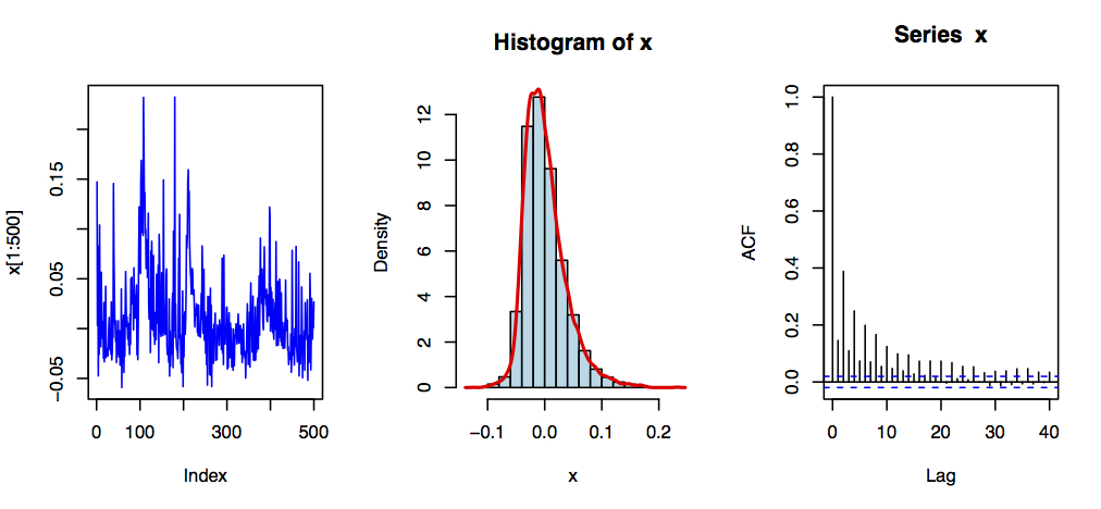
Figure 1: The process obtained by aggregating $N=5000$ independent random-coefficient AR(1) with the Gamma noise in (4.19) and mixing density (4.21), $\beta=0.75$. [left] the first $500$ values of the simulated trajectory, [Middle] histogram, [right] empirical auto covariance. The sample size $n=10000$.

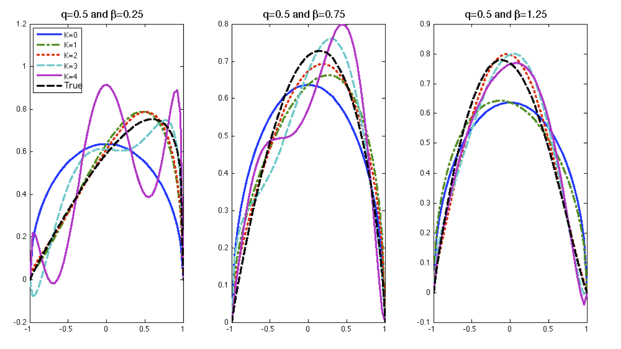
Figure 2: The estimates $\widehat{\phi}_{n}$ computed from the aggregated series with $N=5000$ and Gamma noise (4.19). The mixing density is (4.21). [left] $\beta=0.25$,  [middle] $\beta=0.75$,  [right] $\beta=1.25$. The sample size $n=10000$.

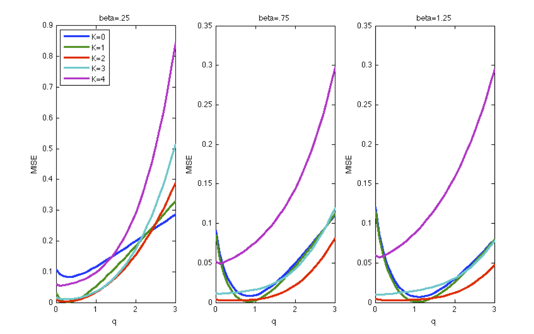
Figure 3: The estimated MISE of $\widehat{\phi}_{n}$ versus $q$ computed from the aggregated series with $N=5000$ and the Gamma noise in (4.19). The true density is (4.21). [left] $\beta=0.25$,  [middle] $\beta=0.75$,  [right] $\beta=1.25$. The number of replications is 500. The sample size $n=10000$.

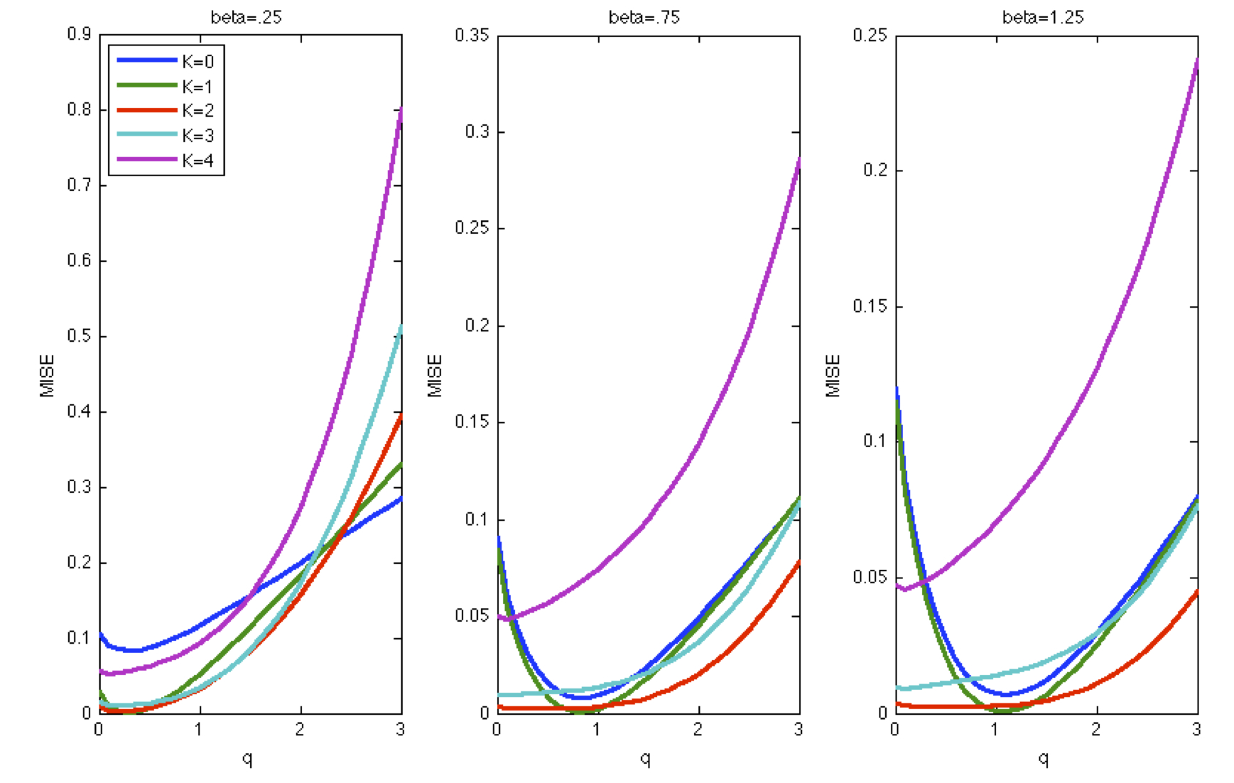
Figure 4: The estimated MISE of $\widehat{\phi}_{n}$ versus $q$ computed from the aggregated series with $N=5000$ and Gaussian noise (4.20). The true density is (4.21). [left] $\beta=0.25$,  [middle] $\beta=0.75$,  [right] $\beta=1.25$. The number of replications is 500. The sample size $n=10000$.

References

Abramovitz, M. and Stegun, I., (1965). Handbook of Mathematical Functions with Formulas, Graphs, and Mathematical Tables. Dover, New York.

Beran, J., Schuetzner, M. and Ghosh, S., (2010). From short to long memory: Aggregation and estimation. Comput. Stat. Data Anal. 54, 2432–2442.

Bhansali, R.J., Giraitis, L. and Kokoszka, P., (2007). Approximations and limit theory for quadratic forms of linear processes. Stoch. Proc. Appl. 117, 71–95.

Billingsley, P., (1968). Convergence of Probability Measures. Wiley, New York.

Brandt, A., (1986). The stochastic equation $Y_{n+1}=A_{n}Y_{n}+B_{n}$ with stationary coefficients. Adv. Appl. Prob. 17, 211–220.

Celov, D., Leipus, R. and Philippe, A., (2007). Time series aggregation, disaggregation and long memory. Lithuanian Math. J. 47, 379–393.

Celov, D., Leipus, R. and Philippe, A., (2010). Asymptotic normality of the mixture density estimator in a disaggregation scheme. J. Nonparametric Statist. 22, 425–442.

Cox, D.R., (1984). Long-range dependence: a review. In: H. A. David and H. T. David (Eds.) Statistics: An Appraisal. Iowa State University Press, Iowa, 55–74.

Feller, W., (1966). An Introduction to Probability Theory and Its Applications, vol. 2. Wiley, New York.

Gonçalves, E. and Gouriéroux, C., (1988). Aggrégation de processus autoregressifs d’ordre 1. Annales d’Economie et de Statistique 12, 127–149.

Granger, C.W.J., (1980). Long memory relationship and the aggregation of dynamic models. J. Econometrics 14, 227–238.

Ibragimov, I.A. and Linnik, Yu.V., (1971). Independent and Stationary Sequences of Random Variables. Wolters-Noordhoff, Groningen.

Lavancier, F., (2005). Long memory random fields. In: P. Bertail, P. Doukhan, P. Soulier (Eds.), Dependence in Probability and Statistics. Lecture Notes in Statistics, vol. 187, pp.195–220. Springer, Berlin.

Lavancier, F., (2011). Aggregation of isotropic random fields. J. Statist. Plan. Infer. 141, 3862–3866.

Lavancier, F., Leipus, R. and Surgailis, D., (2012). Aggregation of anisotropic random-coefficient autoregressive random field. Preprint.

Leipus, R. and Surgailis, D. (2003) Random coefficient autoregression, regime switching and long memory. Adv. Appl. Probab. 35 , 1–18.

Leipus, R., Oppenheim, G., Philippe, A. and Viano, M.-C., (2006). Orthogonal series density estimation in a disaggregation scheme. J. Statist. Plan. Inf. 136, 2547–2571.

Leonenko, N. and Taufer, E., (2013). Disaggregation of spatial autoregressive processes. J. Spatial Statistics (in press).

Mikosch, T., Resnick, S., Rootzén, H. and Stegeman, A., (2002). Is network traffic approximated by stable Lévy motion or fractional Brownian motion? Ann. Appl. Probab., 12, 23–68.

Puplinskaitė, D. and Surgailis, D., (2012). Aggregation of autoregressive random fields and anisotropic long memory. Preprint.

Puplinskaitė, D. and Surgailis, D., (2009). Aggregation of random coefficient AR1(1) process with infinite variance and common innovations. Lithuanian Math. J. 49, 446–463.

Puplinskaitė, D. and Surgailis, D., (2010). Aggregation of random coefficient AR1(1) process with infinite variance and idiosyncratic innovations. Adv. Appl. Probab. 42, 509–527.

Reed, M. and Simon, B., (1975). Methods of Modern Mathematical Physics, vol.2. Academic Press, New York.

Robinson, P. (1978) Statistical inference for a random coefficient autoregressive model. Scand. J. Statist. 5, 163–168.

Rajput, B. S. and Rosinski, J., (1989). Spectral representations of infinitely divisible processes. Probab. Th. Rel. Fields 82, 451–487.

Oppenheim, G. and Viano, M.-C., (2004). Aggregation of random parameters Ornstein-Uhlenbeck or AR processes: some convergence results. J. Time Ser. Anal. 25, 335–350.

Sato, K.-I., (1999). Lévy processes and Infinitely Divisible Distributions. Cambridge Univ. Press, Cambridge.

Surgailis, D. (1981) On infinitely divisible self-similar random fields. Zeit. Wahrsch. verw. Geb. 58, 453–477.

Zaffaroni, P. (2004) Contemporaneous aggregation of linear dynamic models in large economies. J. Econometrics 120, 75–102.