Revisiting the concentration problem of vector fields within a spherical cap: a commuting differential operator solution

Abstract

We propose a novel basis of vector functions, the mixed vector spherical harmonics that are closely related to the functions of Sheppard and Török and help us reduce the concentration problem of tangential vector fields within a spherical cap to an equivalent scalar problem. Exploiting an analogy with previous results published by Grünbaum and his colleagues, we construct a differential operator that commutes with the concentration operator of this scalar problem and propose a stable and convenient method to obtain its eigenfunctions. Having obtained the scalar eigenfunctions, the calculation of tangential vector Slepian functions is straightforward.

Keywords: concentration problem, spherical cap, commuting differential operator, vector spherical harmonics; bandlimited function, eigenvalue problem

Mathematics Subject Classification: 33C47, 33F05, 34B24, 42C10, 47B32

1 Introduction

In our mathematical models, we often assume bandlimitedness for physical or computational reasons, yet also wish that our solutions be localized, with respect to their energy, inside a finite spatial region. Since these are mutually exclusive conditions [29], we need to resort to bandlimited functions with an optimal spatial localization. The goal of the so-called spatial concentration problem [22, p. 75] is to find such functions, and since its first thorough investigation by Slepian, Landau and Pollak in one and multiple Cartesian dimensions [30, 14, 15, 28], it has been revisited many times, including solutions for spherical and planar regions of arbitrary shape [10, 1, 26, 27].

Each individual concentration problem gives rise to an orthogonal set of well-localized functions, which now we refer to under the common name Slepian functions. They have enjoyed increasing popularity in applications involving signal processing, function representation and approximation or the solution of inverse problems. In particular, the scalar spherical Slepian functions have been utilized, for instance, in geodesy and geophysics [1, 26, 27, 25, 11], cosmology [5, 6], computer science [16] and mathematics [19].

While they have been widely applied in the last two decades, it was not until recently that the theory of vector Slepian functions began to mature. The first successful construction of bandlimited vector fields, localized to a spherical cap, was reported in the context of biomedical science [18], followed by an application in physical optics [13]. Recently, a more general treatment of the vector spherical concentration problem has been published [23], however, the question on the existence of a commuting differential operator for the spherical cap has been left unresolved. This question is important for the following reasons.

Slepian functions of a particular problem are eigenfunctions of the so-called concentration operator associated with the spatial region of interest, an integral operator exhibiting a peculiar step-like eigenvalue spectrum. This property makes the direct calculation of its eigenfunctions numerically difficult [4].

A particularly important result of Slepian and his colleagues was the introduction of a Sturm–Liouville differential operator that commutes with the corresponding concentration operator, hence they share a common set of eigenfunctions. Since the differential operator has a simple spectrum with more evenly distributed eigenvalues, it allows a more stable and accurate numerical computation of the eigenfunctions [4]. Two decades after the seminal papers by Slepian and his colleagues, Grünbaum, Longhi and Perlstadt found such a commuting differential operator for the scalar concentration problem within a spherical cap as well [10]. However, we are not aware of a similar proposal for the vectorial problem.

In this paper, we construct a differential operator commuting with the concentration operator of the vector case. This constitutes our main result. We restrict ourselves to tangential vector fields, since the concentration problem of the radial component is equivalent to the scalar concentration problem on the sphere [23], which has already been studied extensively [26]. The key functions in our investigations are the novel mixed vector spherical harmonics $\bm{\mathrm{Q}}_{lm}^{\pm}(\theta,\phi)$ which enable us to reduce the vectorial problem to a scalar one involving the special functions $F_{lm}$ of Sheppard and Török [24]. After that, the problem can be solved in an analogous way to its scalar counterpart [26].

We note that we only consider spatially localized, bandlimited fields here. The symmetric problem of spectrally concentrated, spacelimited functions can be derived by exploiting the analogy to previously published results [26, 23].

2 Preliminaries: associated special functions

In preparation for the concentration problem, we give a detailed survey on the essential properties of important special functions used in our investigations. We start by revisiting the key properties of the normalized associated Legendre functions, because they provide a foundation for the theory of the special functions $F_{lm}$. After that, we prove several fundamental relations for $F_{lm}$, such as orthonormality and recurrence relations, and Christoffel–Darboux formula.

Next we diagonalize the vector Laplacian on the spherical surface and introduce the mixed vector spherical harmonics. We establish a relation between them and the functions $F_{lm}$ and discuss their orthogonality properties. Finally we show how to expand an arbitrary tangential vector field in terms of the mixed vector spherical harmonics and define bandlimitedness in this context, so that we can use these new vector fields as basis functions in the treatment of the concentration problem in Section 3.

2.1 Normalized associated Legendre functions

2.1.1 Definition and orthonormality

The normalized associated Legendre functions $U_{lm}$ of integer degree $l$ and order $m$ are defined as [3, p. 757]

$$U_{lm}(x):=c_{lm}P_{l}^{m}(x),\quad l\geq 0,-l\leq m\leq l,$$ (1)

where

$$P_{l}^{m}(x):=\frac{(-1)^{m}}{2^{l}l!}(1-x^{2})^{m/2}\frac{\operatorname{d}\!^{l+m}}{\operatorname{d}\!x^{l+m}}(x^{2}-1)^{l}$$ (2)

are the (unnormalized) associated Legendre functions [3, p. 743], and

$$c_{lm}:=\sqrt{\frac{2l+1}{2}\frac{(l-m)!}{(l+m)!}}$$ (3)

is the normalization factor.

The normalized associated Legendre functions satisfy the orthonormality relation

$$\int_{-1}^{1}U_{lm}(x)U_{l^{\prime}m}(x)\operatorname{d}\!x=\delta_{ll^{\prime}},$$ (4)

where $\delta_{ll^{\prime}}$ is the Kronecker delta.

2.1.2 Recurrence relations

We can obtain recurrence relations for $U_{lm}$ in a straightforward way by transforming the corresponding relations for $P_{l}^{m}$ [3, p. 744]:

$$xU_{lm}(x) =\xi_{lm}U_{l-1,m}(x)+\xi_{l+1,m}U_{l+1,m}(x),$$ (5)

$$(1-x^{2})\frac{\operatorname{d}\!U_{lm}(x)}{\operatorname{d}\!x} =-lxU_{lm}(x)+(2l+1)\xi_{lm}U_{l-1,m}(x),$$ (6)

$$(1-x^{2})\frac{\operatorname{d}\!U_{lm}(x)}{\operatorname{d}\!x} =(l+1)xU_{lm}(x)-(2l+1)\xi_{l+1,m}U_{l+1,m}(x),$$ (7)

where

$$\xi_{lm}:=\frac{l+m}{2l+1}\frac{c_{lm}}{c_{l-1,m}}=\sqrt{\frac{(l+m)(l-m)}{(2l+1)(2l-1)}}.$$ (8)

In addition, two more recurrence relations can be formulated [8, 17]:

$$-\sqrt{1-x^{2}}\,\frac{\operatorname{d}\!U_{lm}(x)}{\operatorname{d}\!x}=a_{lm}^{+}U_{l,m+1}(x)+a_{lm}^{-}U_{l,m-1}(x),$$ (9a)

where

$$a_{lm}^{\pm}:=\pm\frac{\sqrt{(l\mp m)(l\pm m+1)}}{2},$$ (9b)

and

$$\frac{mU_{lm}(x)}{\sqrt{1-x^{2}}}=b_{lm}^{+}U_{l-1,m+1}(x)+b_{lm}^{-}U_{l-1,m-1}(x),$$ (10a)

where

$$b_{lm}^{\pm}:=-\sqrt{\frac{2l+1}{2l-1}}\frac{\sqrt{(l\mp m)(l\mp m-1)}}{2}.$$ (10b)

Note that everywhere in this paper, where the $\pm$ or $\mp$ signs occur, either the upper or the lower one has to be used consistently in the whole expression.

2.1.3 Differential equation and symmetries

The functions $U_{lm}$ are solutions to the Sturm–Liouville differential equation [3, p. 744]

$$\frac{\operatorname{d}\!}{\operatorname{d}\!x}\left[(1-x^{2})\frac{\operatorname{d}\!u(x)}{\operatorname{d}\!x}\right]-\frac{m^{2}}{1-x^{2}}u(x)=-l(l+1)u(x),$$ (11)

known as the associated Legendre equation. Since it contains $m^{2}$ only, $U_{lm}$ and $U_{l,-m}$ must be proportional. In fact, they are related by the symmetry relation [3, p. 743]

$$U_{l,-m}(x)=(-1)^{m}U_{lm}(x).$$ (12)

In addition, we can formulate the parity relation [3, p. 746]

$$U_{lm}(-x)=(-1)^{l+m}U_{lm}(x).$$ (13)

2.1.4 Special values

There exist closed-form expressions for special arguments or parameter values of $U_{lm}$. At the interval endpoints, $U_{lm}$ evaluates to [3, p. 746]

$$U_{lm}(\pm 1)=\begin{cases}(\pm 1)^{l}c_{l,0}&\quad\text{if $m=0$,}\\ 0&\quad\text{otherwise}.\end{cases}$$ (14)

Another expression for the case $l=m$ is [3, p. 745]

$$U_{mm}(x)=(-1)^{m}c_{mm}\,(2m-1)!!\,(1-x^{2})^{m/2},\quad m\geq 0,$$ (15)

where $(2m-1)!!=(2m-1)(2m-3)\cdots(1)$ is the double factorial. Equation (15) can be used as an initial value to obtain $U_{lm}(x)$ numerically in a fast and stable way [9, p. 364]. Considering $m\geq 0$, we set $U_{m-1,m}(x)=0$ and calculate $U_{mm}(x)$. We then use recurrence relation (5) in the upward direction until we reach $U_{lm}(x)$. Function values for $m<0$ can be obtained using symmetry relation (12).

2.1.5 Addition theorems

Based on the work of Winch and Roberts [34], we can formulate two addition theorems which will be useful later:

$$(1-x^{2})\sum_{m=-l}^{l}\left[\frac{\operatorname{d}\!U_{lm}(x)}{\operatorname{d}\!x}\right]^{2}=\frac{l(l+1)(2l+1)}{4},$$ (16a)

$$\frac{1}{1-x^{2}}\sum_{m=-l}^{l}\bigl{[}mU_{lm}(x)\bigr{]}^{2}=\frac{l(l+1)(2l+1)}{4}.$$ (16b)

2.2 Special functions $F_{lm}$ of Sheppard and Török

2.2.1 Definition and orthonormality

In this section, we give a detailed description of the functions

$$F_{lm}(x):=\frac{1}{\sqrt{l(l+1)}}\left[\sqrt{1-x^{2}}\frac{\operatorname{d}\!U_{lm}(x)}{\operatorname{d}\!x}-\frac{m}{\sqrt{1-x^{2}}}U_{lm}(x)\right],\quad l\geq 1,-m\leq l\leq m,$$ (17)

previously defined by Sheppard and Török [24]. We can express the conditions for the integer indices $l$ and $m$ alternatively as $-\infty<m<\infty$ and $l\geq\ell_{m}$, where the minimal degree $\ell_{m}$ for a fixed $m$ is

$$\ell_{m}:=\max(1,{\lvert m\rvert}).$$ (18)

The functions $F_{lm}$ are orthonormal over $[-1,1]$ for fixed $m$, i.e.

$$\int_{-1}^{1}F_{lm}(x)F_{l^{\prime}m}(x)\operatorname{d}\!x=\delta_{ll^{\prime}},$$ (19)

as shown in A.1. A small subset of them ($l\leq 3$) is described in Fig. 1.

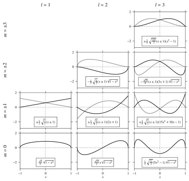
Figure 1: The functions $F_{lm}(x)$ for $l\leq 3$. For ${\lvert m\rvert}>0$, the black and gray curves correspond to the function of positive and negative values of $m$, respectively.

We can obtain useful equivalent formulations of $F_{lm}$ by inserting recurrence relations (6) or (7) of $U_{lm}$ into (17):

$$F_{lm}(x) =\frac{-(lx+m)U_{lm}(x)+(2l+1)\xi_{lm}U_{l-1,m}(x)}{\sqrt{l(l+1)}\sqrt{1-x^{2}}},$$ (20)

$$F_{lm}(x) =\frac{\bigl{[}(l+1)x-m\bigr{]}U_{lm}(x)-(2l+1)\xi_{l+1,m}U_{l+1,m}(x)}{\sqrt{l(l+1)}\sqrt{1-x^{2}}}.$$ (21)

Sometimes it is inconvenient that expressions (17), (20), and (21) are all singular at $x=\pm 1$ because of the factor $(1-x^{2})^{-1/2}$. However, a singularity-free form can also be obtained by exploiting recurrence relations (9b) and (10b):

$$F_{lm}(x)=\frac{-1}{\sqrt{l(l+1)}}\left[a_{lm}^{+}U_{l,m+1}(x)+a_{lm}^{-}U_{l,m-1}(x)+b_{lm}^{+}U_{l-1,m+1}(x)+b_{lm}^{-}U_{l-1,m-1}(x)\right].$$ (22)

It is straightforward to show using (12) and (22) that for the special case $m=0$, the equivalence $F_{l,0}(x)=-U_{l,1}(x)$ holds.

2.2.2 Recurrence relations and Christoffel–Darboux formula

We have found the following recurrence relations for $F_{lm}$ (cf. the corresponding relations (5)–(7) of $U_{lm}$):

$$\left[x-\frac{m}{l(l+1)}\right]F_{lm}(x) =\zeta_{lm}F_{l-1,m}(x)+\zeta_{l+1,m}F_{l+1,m}(x),$$ (23)

$$(1-x^{2})\frac{\operatorname{d}\!F_{lm}(x)}{\operatorname{d}\!x} =-l\left(x-\frac{m}{l^{2}}\right)F_{lm}(x)+(2l+1)\zeta_{lm}F_{l-1,m}(x),$$ (24)

$$(1-x^{2})\frac{\operatorname{d}\!F_{lm}(x)}{\operatorname{d}\!x} =(l+1)\left[x-\frac{m}{(l+1)^{2}}\right]F_{lm}(x)-(2l+1)\zeta_{l+1,m}F_{l+1,m}(x),$$ (25)

where

$$\zeta_{lm}:=\frac{\sqrt{(l+1)(l-1)}}{l}\,\xi_{lm}=\frac{1}{l}\sqrt{\frac{(l+1)(l-1)(l+m)(l-m)}{(2l+1)(2l-1)}}.$$ (26)

A proof for (23) and (24) is provided in A.2 and A.3, respectively. Relation (25) is straightforward to prove by combining (23) and (24).

Relation (23) can also be used to derive a Christoffel–Darboux formula [32, p. 42] specialized for $F_{lm}$:

$$(x-x^{\prime})\sum_{l=\ell_{m}}^{L}F_{lm}(x)F_{lm}(x^{\prime})=\zeta_{L+1,m}\bigl{[}F_{L+1,m}(x)F_{Lm}(x^{\prime})-F_{Lm}(x)F_{L+1,m}(x^{\prime})\bigr{]}.$$ (27)

See A.4 for the details.

2.2.3 Differential equation and symmetry

The functions $F_{lm}$ satisfy the Sturm–Liouville differential equation

$$\frac{\operatorname{d}\!}{\operatorname{d}\!x}\left[(1-x^{2})\frac{\operatorname{d}\!u(x)}{\operatorname{d}\!x}\right]-\frac{m^{2}-2mx+1}{1-x^{2}}u(x)=-l(l+1)u(x),$$ (28)

as proven in A.5. Comparing its symmetry properties to those of the associated Legendre equation (11), we find an important difference: while (11) is invariant under a change in the sign of $m$, in (28) the signs of both $m$ and $x$ have to be changed for transformation invariance. In fact, by inserting symmetry relation (12) of $U_{lm}$ into definition (17) of $F_{lm}$ and exploiting the parity relation (13), we get the following symmetry relation for $F_{lm}$:

$$F_{l,-m}(-x)=(-1)^{l+1}F_{lm}(x).$$ (29)

This symmetry relation is also apparent in Fig. 1.

2.2.4 Special values

Combining $U_{lm}(\pm 1)$ of (14) and the singularity-free form (22) of $F_{lm}$ provides a simple way to calculate the function values at the endpoints $x=\pm 1$:

$$F_{lm}(1) =\begin{cases}c_{l,0}&\quad\text{if $m=1$,}\\ 0&\quad\text{otherwise,}\end{cases}$$ (30a)

$$F_{lm}(-1) =\begin{cases}(-1)^{l-1}c_{l,0}&\quad\text{if $m=-1$,}\\ 0&\quad\text{otherwise.}\end{cases}$$ (30b)

In addition, to get a relation similar to the closed-form expression (15) for $U_{mm}$, we can combine  (15) with definition (17) of $F_{lm}$. In this way we obtain

$$F_{\ell_{m},m}(x)=\begin{cases}(-1)^{m+1}(1+x)\Phi_{m}(x)\qquad&\text{if $m>0$,}\\ \frac{\sqrt{3}}{2}\sqrt{1-x^{2}}\qquad&\text{if $m=0$,}\\ (1-x)\Phi_{{\lvert m\rvert}}(x)\qquad&\text{if $m<0$,}\end{cases}$$ (31)

where

$$\Phi_{m}(x):=\sqrt{\frac{m}{m+1}}\,c_{mm}\,(2m+1)!!\,(1-x^{2})^{(m-1)/2}.$$ (32)

Like in the case of the associated Legendre functions, recurrence relation (23) provides a stable and efficient method to evaluate $F_{lm}(x)$ numerically. By setting $F_{\ell_{m}-1,m}=0$ and starting with the closed-form expression (31) for $F_{\ell_{m},m}(x)$, recurrence relation (23) can be used repeatedly in the upward direction until one obtains $F_{lm}(x)$.

2.2.5 Addition theorem

We can use the addition theorems (16) of $U_{lm}(x)$ to formulate a similar relation for $F_{lm}(x)$ as well:

$$\sum_{m=-l}^{l}\bigl{[}F_{lm}(x)\bigr{]}^{2}=\frac{2l+1}{2}.$$ (33)

The proof can be found in A.6.

2.3 Scalar and vector Laplacian on the unit sphere

Let $u=u(\theta,\phi)$ be an arbitrary scalar field and $\bm{\mathrm{v}}=v_{\theta}(\theta,\phi)\hat{\bm{\mathrm{\theta}}}+v_{\phi}(\theta,\phi)\hat{\bm{\mathrm{\phi}}}$ a (tangential) vector field defined on the unit sphere

$$\Omega:=\left\{(\theta,\phi):0\leq\theta\leq\pi,\ 0\leq\phi<2\pi\right\}\,.$$ (34)

Here, $\hat{\bm{\mathrm{\theta}}}$ and $\hat{\bm{\mathrm{\phi}}}$ are unit vectors in the $\theta$- and $\phi$-directions, respectively, as shown in Fig. 2.

Figure 2: Sketch of the unit sphere $\Omega$ showing Cartesian unit vectors $\hat{\bm{\mathrm{x}}}$, $\hat{\bm{\mathrm{y}}}$, $\hat{\bm{\mathrm{z}}}$, and the polar and azimuthal unit vectors $\hat{\bm{\mathrm{\theta}}}$ and $\hat{\bm{\mathrm{\phi}}}$, respectively.

The surface scalar and vector Laplacian on $\Omega$ are defined as follows [31]:

$$\nabla_{\Omega}^{2}\,u :=\frac{1}{\sin\theta}\frac{\partial}{\partial\theta}\left(\sin\theta\frac{\partial u}{\partial\theta}\right)+\frac{1}{\sin^{2}\theta}\,\frac{\partial^{2}u}{\partial\phi^{2}},$$ (35)

$$\nabla_{\Omega}^{2}\,\bm{\mathrm{v}} :=\left[\nabla_{\Omega}^{2}v_{\theta}-\frac{v_{\theta}}{\sin^{2}\theta}-2\frac{\cos\theta}{\sin^{2}\theta}\frac{\partial v_{\phi}}{\partial\phi}\right]\hat{\bm{\mathrm{\theta}}}+\left[\nabla_{\Omega}^{2}v_{\phi}-\frac{v_{\phi}}{\sin^{2}\theta}\,+2\frac{\cos\theta}{\sin^{2}\theta}\frac{\partial v_{\theta}}{\partial\phi}\right]\hat{\bm{\mathrm{\phi}}}.$$ (36)

Note that the each component of $\nabla_{\Omega}^{2}\,\bm{\mathrm{v}}$ contains both components of $\bm{\mathrm{v}}$. We can diagonalize $\nabla_{\Omega}^{2}\,\bm{\mathrm{v}}$ by introducing the tangential basis vectors

$$\hat{\bm{\mathrm{\tau}}}_{\pm}:=\frac{1}{\sqrt{2}}\bigl{(}\hat{\bm{\mathrm{\theta}}}\pm\mathrm{i}\,\hat{\bm{\mathrm{\phi}}}\bigr{)},$$ (37)

which are orthogonal with respect to the complex dot product

$$\hat{\bm{\mathrm{\tau}}}^{\ast}_{\pm}\cdot\hat{\bm{\mathrm{\tau}}}_{\mp}=0.$$ (38)

Here $\mathrm{i}$ is the imaginary unit and the asterisk denotes the complex conjugate.

In this new basis, we can write (36) as

$$\nabla_{\Omega}^{2}\,\bm{\mathrm{v}}=\bigl{(}\Delta_{\Omega}^{+}v_{+}\bigr{)}\hat{\bm{\mathrm{\tau}}}_{+}+\bigl{(}\Delta_{\Omega}^{-}v_{-}\bigl{)}\hat{\bm{\mathrm{\tau}}}_{-},$$ (39)

where $\bm{\mathrm{v}}=v_{+}(\theta,\phi)\hat{\bm{\mathrm{\tau}}}_{+}+v_{-}(\theta,\phi)\hat{\bm{\mathrm{\tau}}}_{-}$ and

$$\Delta_{\Omega}^{\pm}:=\nabla_{\Omega}^{2}-\frac{1}{\sin^{2}\theta}\left(1\pm 2\mathrm{i}\cos\theta\frac{\partial}{\partial\phi}\right).$$ (40)

Next we introduce two fixed-order operators, which play a central role in constructing commuting differential operators for the spherical cap, as we will see in Section 3.3. For separable functions of the form $u(\theta,\phi)=w(\theta)\exp(\mathrm{i}m\phi)$ the differentiation with respect to $\phi$ can be performed explicitly, and the scalar operators $\nabla_{\Omega}^{2}$, $\Delta_{\Omega}^{+}$ and $\Delta_{\Omega}^{-}$ become identical to the following fixed-order operators $\nabla_{\Omega,m}^{2}$, $\Delta_{\Omega,m}$ and $\Delta_{\Omega,-m}$, respectively:

$$\nabla_{\Omega,m}^{2} :=\frac{1}{\sin\theta}\frac{\operatorname{d}\!}{\operatorname{d}\!\theta}\left(\sin\theta\frac{\operatorname{d}\!}{\operatorname{d}\!\theta}\right)-\frac{m^{2}}{\sin^{2}\theta},$$ (41)

$$\Delta_{\Omega,\pm m} :=\nabla_{\Omega,\pm m}^{2}-\frac{1-2(\pm m)\cos\theta}{\sin^{2}\theta}.$$ (42)

Since $\nabla_{\Omega,m}^{2}=\nabla_{\Omega,-m}^{2}$, we can write (42) in a more compact form:

$$\Delta_{\Omega,m}:=\nabla_{\Omega,m}^{2}-\frac{1-2m\cos\theta}{\sin^{2}\theta}.$$ (43)

Upon substituting $x=\cos\theta$ in $\nabla_{\Omega,m}^{2}$ and $\Delta_{\Omega,m}$, we regain the differential operators on the left-hand side of differential equations (11) and (28), respectively. Therefore $U_{lm}$ and $F_{lm}$ satisfy the eigenvalue equations

$$\nabla_{\Omega,m}^{2}U_{lm}(\cos\theta) =-l(l+1)U_{lm}(\cos\theta),$$ (44)

$$\Delta_{\Omega,m}F_{lm}(\cos\theta) =-l(l+1)F_{lm}(\cos\theta).$$ (45)

2.4 Mixed vector spherical harmonics

2.4.1 Definition and orthonormality

We define the mixed vector spherical harmonics as

$$\bm{\mathrm{Q}}_{lm}^{\pm}(\theta,\phi):=\frac{(\pm 1)^{m+1}}{\sqrt{2}}\bigl{[}\bm{\mathrm{Y}}_{lm}(\theta,\phi)\pm\mathrm{i}\,\bm{\mathrm{Z}}_{lm}(\theta,\phi)\bigr{]},$$ (46)

where $\bm{\mathrm{Y}}_{lm}$ and $\bm{\mathrm{Z}}_{lm}$ are the conventional (fully normalized) tangential vector spherical harmonics. They are defined as [20, 13]

$$\bm{\mathrm{Y}}_{lm}(\theta,\phi) :=\frac{\mathrm{i}}{\sqrt{l(l+1)}}\left[\frac{1}{\sin\theta}\frac{\partial Y_{lm}(\theta,\phi)}{\partial\phi}\hat{\bm{\mathrm{\theta}}}-\frac{\partial Y_{lm}(\theta,\phi)}{\partial\theta}\hat{\bm{\mathrm{\phi}}}\right],$$ (47a)

$$\bm{\mathrm{Z}}_{lm}(\theta,\phi) :=\frac{\mathrm{i}}{\sqrt{l(l+1)}}\left[\frac{\partial Y_{lm}(\theta,\phi)}{\partial\theta}\hat{\bm{\mathrm{\theta}}}+\frac{1}{\sin\theta}\frac{\partial Y_{lm}(\theta,\phi)}{\partial\phi}\hat{\bm{\mathrm{\phi}}}\right],$$ (47b)

where

$$Y_{lm}(\theta,\phi):=U_{lm}(\cos\theta)\frac{\exp(\mathrm{i}m\phi)}{\sqrt{2\pi}}$$ (48)

are the scalar spherical harmonics.

Equations (17), (37), (47) and (48) can be used to write (46) in a separable form:

$$\bm{\mathrm{Q}}_{lm}^{\pm}(\theta,\phi)=F_{l,\pm m}(\cos\theta)\frac{\exp(\mathrm{i}m\phi)}{\sqrt{2\pi}}\,\hat{\bm{\mathrm{\tau}}}_{\pm}.$$ (49)

It directly follows from this formulation and the orthogonality of $\hat{\bm{\mathrm{\tau}}}_{\pm}$ that, unlike $\bm{\mathrm{Y}}_{lm}$ and $\bm{\mathrm{Z}}_{lm}$, the functions $\bm{\mathrm{Q}}_{lm}^{\pm}$ exhibit local (vector) orthogonality, regardless of their degree and order, i.e.

$$\bm{\mathrm{Q}}_{lm}^{\pm\,*}(\theta,\phi)\cdot\bm{\mathrm{Q}}_{l^{\prime}m^{\prime}}^{\mp}(\theta,\phi)=0.$$ (50)

This equation together with (49) can be used to prove the orthonormality relations

$$\int_{\Omega}\bm{\mathrm{Q}}_{lm}^{\pm\,*}(\theta,\phi)\cdot\bm{\mathrm{Q}}_{l^{\prime}m^{\prime}}^{\pm}(\theta,\phi)\,\operatorname{d}\!\Omega =\delta_{ll^{\prime}}\delta_{mm^{\prime}},$$ (51a)

$$\int_{\Omega}\bm{\mathrm{Q}}_{lm}^{\pm\,*}(\theta,\phi)\cdot\bm{\mathrm{Q}}_{l^{\prime}m^{\prime}}^{\mp}(\theta,\phi)\,\operatorname{d}\!\Omega =0,$$ (51b)

where $\int_{\Omega}\dots\operatorname{d}\!\Omega:=\int_{0}^{2\pi}\int_{0}^{\pi}\dots\sin\theta\operatorname{d}\!\theta\operatorname{d}\!\phi$.

2.4.2 Special values

The values of $\bm{\mathrm{Q}}_{lm}^{\pm}$ at the $\theta$-coordinate singularities deserve extra attention, since $\hat{\bm{\mathrm{\tau}}}_{\pm}$ are not well defined there. We can circumvent this problem by expressing $\bm{\mathrm{Q}}_{lm}^{\pm}$ using Cartesian basis vectors (see Fig. 2). Using Eqs. (30) for $F_{lm}(\pm 1)$, we have

$$\bm{\mathrm{Q}}_{lm}^{\pm}(\theta=0,\phi) =\begin{cases}\frac{1}{2\sqrt{\pi}}c_{l,0}(\hat{\bm{\mathrm{x}}}\pm\mathrm{i}\hat{\bm{\mathrm{y}}})&\text{if $m=\pm 1$},\\ 0&\text{otherwise},\end{cases}$$ (52a)

$$\bm{\mathrm{Q}}_{lm}^{\pm}(\theta=\pi,\phi) =\begin{cases}\frac{(-1)^{l}}{2\sqrt{\pi}}c_{l,0}(\hat{\bm{\mathrm{x}}}\mp\mathrm{i}\hat{\bm{\mathrm{y}}})&\text{if $m=\mp 1$},\\ 0&\text{otherwise}.\end{cases}$$ (52b)

2.4.3 Spherical harmonic expansion and bandlimited functions

Like $\bm{\mathrm{Y}}_{lm}$ and $\bm{\mathrm{Z}}_{lm}$ [7], the mixed vector spherical harmonics $\bm{\mathrm{Q}}_{lm}^{\pm}$ also form a complete basis of the Hilbert space of square-integrable tangential vector fields defined over $\Omega$. Hence we can expand an arbitrary tangential vector field $\bm{\mathrm{v}}$ in terms of $\bm{\mathrm{Q}}_{lm}^{\pm}$ as

$$\bm{\mathrm{v}}(\theta,\phi)=\sum_{l=1}^{\infty}\sum_{m=-l}^{l}\left[v_{lm}^{+}\bm{\mathrm{Q}}_{lm}^{+}(\theta,\phi)+v_{lm}^{-}\bm{\mathrm{Q}}_{lm}^{-}(\theta,\phi)\right],$$ (53)

where the expansion coefficients $v_{lm}^{\pm}$ can be calculated as

$$v_{lm}^{\pm}:=\int_{\Omega}\bm{\mathrm{Q}}_{lm}^{\pm\,*}(\theta,\phi)\cdot\bm{\mathrm{v}}(\theta,\phi)\,\operatorname{d}\!\Omega.$$ (54)

If $v_{lm}^{\pm}=0$ for $L<l<\infty$ and some $L>0$, we call $\bm{\mathrm{v}}$ bandlimited. The limit $L$ is the maximal degree of functions $\bm{\mathrm{Q}}_{lm}^{\pm}$ that contribute to the expansion (53). Therefore the subspace $S_{L}$ of bandlimited vector fields is finite dimensional, its dimension is equal to the number of terms in (53):

$$\dim S_{L}=2\sum_{l=1}^{L}(2l+1)=2\bigl{[}(L+1)^{2}-1\bigr{]}=2L(L+2).$$ (55)

3 The concentration problem of tangential vector fields within an axisymmetrical spherical cap

Having defined all important special functions, we now turn our attention to the main topic of the paper. After a brief discussion of the concentration problem in terms of the mixed vector spherical harmonics, we introduce a reduced scalar problem which can be solved analogously to the theory of scalar spherical Slepian functions [10, 26].

In Section 3.2, we analyze the eigenvalue spectrum of the concentration operator and give an illustration on the scalar eigenfunctions.

Finally, we propose a fast and numerically stable way to calculate the eigenfunctions by using a differential operator that commutes with the scalar concentration operator obtained previously.

3.1 Formulation of the vector problem and its reduction to a scalar one

We consider the variational problem of finding a bandlimited, tangential vector field $\bm{\mathrm{G}}(\theta,\phi)\in S_{L}$ that maximizes the fractional energy contained within an axisymmetric spherical cap $C$:

$$\max_{\bm{\mathrm{G}}}\ \frac{\int_{C}{\lvert\bm{\mathrm{G}}(\theta,\phi)\rvert}^{2}\operatorname{d}\!\Omega}{\int_{\Omega}{\lvert\bm{\mathrm{G}}(\theta,\phi)\rvert}^{2}\operatorname{d}\!\Omega}=\max_{\bm{\mathrm{G}}}\ \frac{\int_{C}\bm{\mathrm{G}}^{*}(\theta,\phi)\cdot\bm{\mathrm{G}}(\theta,\phi)\operatorname{d}\!\Omega}{\int_{\Omega}\bm{\mathrm{G}}^{*}(\theta,\phi)\cdot\bm{\mathrm{G}}(\theta,\phi)\operatorname{d}\!\Omega}.$$ (56)

Without loss of generality, we can center our spherical cap at $\theta=0$, as seen in Fig. (3):

$$C=\bigl{\{}(\theta,\phi):0\leq\theta\leq\Theta,0\leq\phi<2\pi\bigr{\}},$$ (57)

where $\Theta>0$ is assumed.

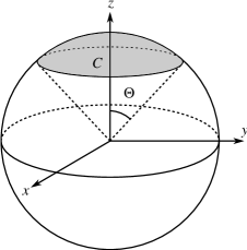
Figure 3: Sketch of the spherical cap $C$.

To solve the vectorial problem (56), we adapt the method of the scalar case [26] and turn (56) into a Rayleigh–Ritz matrix variational problem [12, p. 176]. We can achieve this by expanding $\bm{\mathrm{G}}$ in terms of $\bm{\mathrm{Q}}_{lm}^{\pm}$:

$$\bm{\mathrm{G}}(\theta,\phi)=\sum_{l=1}^{L}\sum_{m=-l}^{l}\left[g_{lm}^{+}\bm{\mathrm{Q}}_{lm}^{+}(\theta,\phi)+g_{lm}^{-}\bm{\mathrm{Q}}_{lm}^{-}(\theta,\phi)\right]=\sum_{m=-L}^{L}\sum_{l=\ell_{m}}^{L}\left[g_{lm}^{+}\bm{\mathrm{Q}}_{lm}^{+}(\theta,\phi)+g_{lm}^{-}\bm{\mathrm{Q}}_{lm}^{-}(\theta,\phi)\right].$$ (58)

In the second step, we have interchanged the order of double summation to facilitate the transition to the matrix formulation of (56) later. A visual comparison of the two summation schemes is given in Fig. 4.

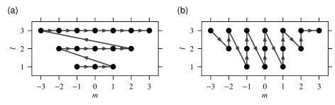
Figure 4: Order of double summation in (a) $\sum_{l=1}^{L}\sum_{m=-l}^{l}$ and (b) $\sum_{m=-L}^{L}\sum_{l=\ell_{m}}^{L}$ for $L=3$, where $\ell_{m}=\max(1,{\lvert m\rvert})$. The filled circles represent terms with corresponding indices $l$ and $m$.

Next we insert (58) into (56), interchange the order of summation and integration and use the orthonormality relations (50) and (51). Hence the numerator can be written as

$$\begin{split}\int_{C}\bm{\mathrm{G}}^{*}(\theta,\phi)\cdot\bm{\mathrm{G}}(\theta,\phi)\operatorname{d}\!\Omega=&\sum_{m=-L}^{L}\sum_{l=\ell_{m}}^{L}g_{lm}^{+\,*}\sum_{m^{\prime}=-L}^{L}\sum_{l^{\prime}=\ell_{m^{\prime}}}^{L}\left[\int_{C}\bm{\mathrm{Q}}_{lm}^{+\,*}(\theta,\phi)\cdot\bm{\mathrm{Q}}_{l^{\prime}m^{\prime}}^{+}(\theta,\phi)\operatorname{d}\!\Omega\right]g_{l^{\prime}m^{\prime}}^{+}\\ &+\sum_{m=-L}^{L}\sum_{l=\ell_{m}}^{L}g_{lm}^{-\,*}\sum_{m^{\prime}=-L}^{L}\sum_{l^{\prime}=\ell_{m^{\prime}}}^{L}\left[\int_{C}\bm{\mathrm{Q}}_{lm}^{-\,*}(\theta,\phi)\cdot\bm{\mathrm{Q}}_{l^{\prime}m^{\prime}}^{-}(\theta,\phi)\operatorname{d}\!\Omega\right]g_{l^{\prime}m^{\prime}}^{-},\end{split}$$ (59)

while the denominator becomes

$$\int_{\Omega}\bm{\mathrm{G}}^{*}(\theta,\phi)\cdot\bm{\mathrm{G}}(\theta,\phi)\operatorname{d}\!\Omega=\sum_{m=-L}^{L}\sum_{l=\ell_{m}}^{L}\left(g_{lm}^{+\,*}g_{lm}^{+}+g_{lm}^{-\,*}g_{lm}^{-}\right).$$ (60)

The integrals on the right-hand side of (59) can be expressed as

$$\int_{C}\bm{\mathrm{Q}}_{lm}^{\pm\,*}(\theta,\phi)\cdot\bm{\mathrm{Q}}_{l^{\prime}m^{\prime}}^{\pm}(\theta,\phi)\operatorname{d}\!\Omega=\frac{1}{2\pi}\int_{0}^{2\pi}\exp\bigl{[}\mathrm{i}(m^{\prime}-m)\phi\bigr{]}\operatorname{d}\!\phi\int_{0}^{\Theta}F_{l,\pm m}(\cos\theta)F_{l^{\prime},\pm m}(\cos\theta)\sin\theta\operatorname{d}\!\theta.$$ (61)

Since $(2\pi)^{-1}\int_{0}^{2\pi}\exp[\mathrm{i}(m^{\prime}-m)\phi]\operatorname{d}\!\phi=\delta_{mm^{\prime}}$, Eq. (61) further simplifies to

$$\int_{C}\bm{\mathrm{Q}}_{lm}^{\pm\,*}(\theta,\phi)\cdot\bm{\mathrm{Q}}_{l^{\prime}m^{\prime}}^{\pm}(\theta,\phi)\operatorname{d}\!\Omega=\delta_{mm^{\prime}}K_{\pm m,ll^{\prime}},$$ (62)

where

$$K_{m,ll^{\prime}}:=\int_{0}^{\Theta}F_{lm}(\cos\theta)F_{l^{\prime}m}(\cos\theta)\sin\theta\operatorname{d}\!\theta=\int_{\cos\Theta}^{1}F_{lm}(x)F_{l^{\prime}m}(x)\operatorname{d}\!x.$$ (63)

The integrand of $K_{m,ll^{\prime}}$ is a polynomial of degree $l+l^{\prime}$, hence it can exactly be integrated numerically, for instance, by a Gauss–Legendre formula of $\lceil(l+l^{\prime}+1)/2\rceil$ nodes.

Taking (62) into account, (56) can be rewritten as

$$\begin{split}\max_{\{g_{lm}^{\pm}\}}\ \Bigg{\{}\ &\left[\sum_{m=-L}^{L}\left(\sum_{l=\ell_{m}}^{L}g_{lm}^{+\,*}\sum_{l^{\prime}=\ell_{m}}^{L}K_{m,ll^{\prime}}g_{l^{\prime}m}^{+}\right)+\sum_{m=-L}^{L}\left(\sum_{l=\ell_{m}}^{L}g_{lm}^{-\,*}\sum_{l^{\prime}=\ell_{m}}^{L}K_{-m,ll^{\prime}}g_{l^{\prime}m}^{-}\right)\right]\\ &\times\ \left[\sum_{m=-L}^{L}\sum_{l=\ell_{m}}^{L}\left(g_{lm}^{+\,*}g_{lm}^{+}+g_{lm}^{-\,*}g_{lm}^{-}\right)\right]^{-1}\ \Bigg{\}}.\end{split}$$ (64)

To express (64) in matrix formalism, we construct a column vector $\mathsf{g}$ of $2L(L+2)$ elements as

$$\mathsf{g}:=\left[g_{L,-L}^{+};g_{L-1,-L+1}^{+},g_{L,-L+1}^{+};\ldots;g_{L,L}^{+};g_{L,-L}^{-};g_{L-1,-L+1}^{-},g_{L,-L+1}^{-};\ldots;g_{L,L}^{-}\right]^{\mathrm{T}}.$$ (65)

where the expansion coefficients $g_{lm}^{\pm}$ are enumerated according to the scheme of Fig. 4b. In addition, we introduce the $2L(L+2)\times 2L(L+2)$ block-diagonal matrix

$$\mathsf{K}:=\begin{bmatrix}\mathsf{K}^{+}&\mathsf{0}\\ \mathsf{0}&\mathsf{K}^{-}\end{bmatrix},$$ (66)

where the $L(L+2)\times L(L+2)$ blocks $\mathsf{K}^{\pm}$ are themselves block-diagonal:

$$\mathsf{K}^{+}:=\operatorname{diag}\left[\mathsf{K}_{-L};\mathsf{K}_{-L+1};\ldots;\mathsf{K}_{L};\right],\qquad\mathsf{K}^{-}:=\operatorname{diag}\left[\mathsf{K}_{L};\mathsf{K}_{L-1};\ldots;\mathsf{K}_{-L}\right].$$ (67)

The elementary blocks

$$\mathsf{K}_{m}=\begin{bmatrix}K_{m,\ell_{m}\ell_{m}}&\cdots&K_{m,\ell_{m}L}\\ \vdots&\ddots&\vdots\\ K_{m,L\ell_{m}}&\cdots&K_{m,LL}\end{bmatrix}$$ (68)

correspond to different orders $m$ and have an order-dependent size of $(L-\ell_{m}+1)\times(L-\ell_{m}+1)$. Note that order of the blocks $\mathsf{K}_{m}$ in $\mathsf{K}^{\pm}$ is reversed owing to (62).

We can thus use these constructions to transform problem (64) into the Rayleigh–Ritz matrix variational problem

$$\max_{\mathsf{g}}\ \frac{\mathsf{g}^{{\dagger}}\,\mathsf{K}\,\mathsf{g}}{\mathsf{g}^{{\dagger}}\,\mathsf{g}},$$ (69)

where the dagger sign denotes the conjugate transpose. Equivalently, we have to find the eigenvector $\mathsf{g}$ of the eigenvalue problem [12, p. 176]

$$\mathsf{K}\mathsf{g}=\eta\,\mathsf{g}$$ (70)

with the maximal eigenvalue $\eta$. However, rather than solving the large $2L(L+2)\times 2L(L+2)$ eigenvalue problem (70), the block-diagonal structure of $\mathsf{K}$ allows us to solve a series of smaller $(L-\ell_{m}+1)\times(L-\ell_{m}+1)$ problems instead,

$$\mathsf{K}_{m}\mathsf{g}_{m}=\eta_{m}\mathsf{g}_{m},\quad-L\leq m\leq L,$$ (71)

one for each order $m$.

From (63) follows that $K_{m,ll^{\prime}}=K_{m,l^{\prime}l}$, implying that the matrices $\mathsf{K}_{m}$ are symmetric. Hence their eigenvalues are always real. For a given $m$, we rank-order the $(L-\ell_{m}+1)$ distinct eigenvalues $\eta_{mn}$ as $1>\eta_{m,1}>\eta_{m,2}>\dots>\eta_{m,L-\ell_{m}+1}>0$. The associated eigenvectors $\mathsf{g}_{mn}$ can be chosen to be real and orthonormal:

$$\mathsf{g}_{mn}^{\mathrm{T}}\mathsf{g}_{mn^{\prime}}=\delta_{nn^{\prime}},\qquad\mathsf{g}_{mn}^{\mathrm{T}}\mathsf{K}_{m}\mathsf{g}_{mn^{\prime}}=\eta_{mn}\delta_{nn^{\prime}},\qquad 1\leq n,n^{\prime}\leq(L-\ell_{m}+1).$$ (72)

Here we have distinguished between the different eigenvalues and the corresponding eigenvectors by the use of the additional index $n$ (or $n^{\prime}$). However, we drop this additional index for brevity when we refer to any of the $(L-\ell_{m}+1)$ eigenvalues or eigenvectors.

We also denote the elements of an eigenvector $\mathsf{g}_{m}$ simply by $g_{lm}$. This brings up the question: how are the coefficients $g_{lm}$ connected to the original coefficients $g_{lm}^{+}$ and $g_{lm}^{-}$ of expansion (58)? According to (66) and (67), each block $\mathsf{K}_{m}$ occurs twice in $\mathsf{K}$, hence each eigenvector $\mathsf{g}_{m}$ gives rise to two vectorial eigenfunctions:

$$\bm{\mathrm{G}}_{m}^{+}(\theta,\phi) =\sum_{l=\ell_{m}}^{L}g_{lm}^{+}\bm{\mathrm{Q}}_{lm}^{+}(\theta,\phi)=\sum_{l=\ell_{m}}^{L}g_{lm}\bm{\mathrm{Q}}_{lm}^{+}(\theta,\phi),$$ (73a)

$$\bm{\mathrm{G}}_{-m}^{-}(\theta,\phi) =\sum_{l=\ell_{-m}}^{L}g_{l,-m}^{-}\bm{\mathrm{Q}}_{l,-m}^{-}(\theta,\phi)=\sum_{l=\ell_{-m}}^{L}g_{lm}\bm{\mathrm{Q}}_{l,-m}^{-}(\theta,\phi).$$ (73b)

Its worth emphasizing that every eigenfunction contains either $\bm{\mathrm{Q}}_{lm}^{+}$ or $\bm{\mathrm{Q}}_{lm}^{-}$ of a single order $m$ only, which is a consequence of the block-diagonal nature of the concentration matrix $\mathsf{K}$. Upon substituting expression (49) of $\bm{\mathrm{Q}}_{lm}^{\pm}$ into Eqs. (73), we obtain

$$\bm{\mathrm{G}}_{\pm m}^{\pm}(\theta,\phi)=G_{m}(\cos\theta)\frac{\exp(\pm\mathrm{i}m\phi)}{\sqrt{2\pi}}\,\hat{\bm{\mathrm{\tau}}}_{\pm},$$ (74)

where

$$G_{m}(x):=\sum_{l=\ell_{m}}^{L}g_{lm}F_{lm}(x)$$ (75)

are real functions.

In this way, we managed to reduce the vectorial concentration problem within a spherical cap to equivalent one-dimensional, scalar concentration problems of various orders $m$. The key idea in this simplification was the choice (49) for our basis functions. The scalar concentration problem for a fixed order $m$ can be formulated as

$$\max_{G_{m}}\frac{\int_{\cos\Theta}^{1}\left[G_{m}(x)\right]^{2}\operatorname{d}\!x}{\int_{-1}^{1}\left[G_{m}(x)\right]^{2}\operatorname{d}\!x},$$ (76)

where $G_{m}$ is a bandlimited scalar function belonging to the subspace spanned by $F_{lm}$. The corresponding Rayleigh–Ritz matrix variational problem is

$$\max_{\mathsf{g}_{m}}\frac{\mathsf{g}_{m}^{\mathrm{T}}\mathsf{K}_{m}\mathsf{g}_{m}}{\mathsf{g}_{m}^{\mathrm{T}}\mathsf{g}_{m}}.$$ (77)

Instead of the eigenvalue equation (71) specifying eigenvectors $\mathsf{g}_{m}$, we can directly formulate an eigenvalue equation in terms of the functions $G_{m}$, too. Therefore we first express Eq. (71) component-wise as

$$\sum_{l^{\prime}=\ell_{m}}^{L}K_{m,ll^{\prime}}g_{l^{\prime}m}=\eta_{m}g_{lm},\quad\ell_{m}\leq l\leq L.$$ (78)

Now we multiply both sides by $F_{lm}(x)$ and sum over $l$:

$$\sum_{l=\ell_{m}}^{L}\sum_{l^{\prime}=\ell_{m}}^{L}K_{m,ll^{\prime}}g_{l^{\prime}m}F_{lm}(x)=\eta_{m}\sum_{l=\ell_{m}}^{L}g_{lm}F_{lm}(x).$$ (79)

The left-hand side can be rewritten as

$$\sum_{l=\ell_{m}}^{L}\sum_{l^{\prime}=\ell_{m}}^{L}K_{m,ll^{\prime}}g_{l^{\prime}m}F_{lm}(x) =\sum_{l=\ell_{m}}^{L}\sum_{l^{\prime}=\ell_{m}}^{L}\left[\int_{\cos\Theta}^{1}F_{lm}(x^{\prime})F_{l^{\prime}m}(x^{\prime})\operatorname{d}\!x^{\prime}\right]g_{l^{\prime}m}F_{lm}(x)$$

$$=\int_{\cos\Theta}^{1}\left\{\left[\,\sum_{l=\ell_{m}}^{L}F_{lm}(x)F_{lm}(x^{\prime})\right]\sum_{l^{\prime}=\ell_{m}}^{L}g_{l^{\prime}m}F_{l^{\prime}m}(x^{\prime})\right\}\operatorname{d}\!x^{\prime}.$$

This way, we obtain a Fredholm integral equation of the second kind for $G_{m}$,

$$\int_{\cos\Theta}^{1}\mathcal{K}_{m}(x,x^{\prime})\,G_{m}(x^{\prime})\operatorname{d}\!x^{\prime}=\eta_{m}G_{m}(x),\quad-1\leq x\leq 1,$$ (80)

where the kernel function $\mathcal{K}_{m}$ is defined as

$$\mathcal{K}_{m}(x,x^{\prime}):=\sum_{l=\ell_{m}}^{L}F_{lm}(x)F_{lm}(x^{\prime}).$$ (81)

It follows from the orthogonality relations (72) of the eigenvectors that the scalar eigenfunctions $G_{m}$ are doubly orthogonal:

$$\int_{-1}^{1}G_{mn}(x)G_{mn^{\prime}}(x)\operatorname{d}\!x =\delta_{nn^{\prime}},$$ (82a)

$$\int_{\cos\Theta}^{1}G_{mn}(x)G_{mn^{\prime}}(x)\operatorname{d}\!x =\eta_{mn}\delta_{nn^{\prime}}.$$ (82b)

The vectorial eigenfunctions $\bm{\mathrm{G}}_{m}^{\pm}$ inherit this property as well:

$$\int_{\Omega}\bm{\mathrm{G}}_{mn}^{\pm\,*}(\theta,\phi)\cdot\bm{\mathrm{G}}_{m^{\prime}n^{\prime}}^{\pm}(\theta,\phi)\,\operatorname{d}\!\Omega =\delta_{mm^{\prime}}\delta_{nn^{\prime}},\quad \int_{\Omega}\bm{\mathrm{G}}_{mn}^{\pm\,*}(\theta,\phi)\cdot\bm{\mathrm{G}}_{m^{\prime}n^{\prime}}^{\mp}(\theta,\phi)\,\operatorname{d}\!\Omega =0,$$ (83a)

$$\int_{C}\bm{\mathrm{G}}_{mn}^{\pm\,*}(\theta,\phi)\cdot\bm{\mathrm{G}}_{m^{\prime}n^{\prime}}^{\pm}(\theta,\phi)\,\operatorname{d}\!\Omega =\eta_{mn}\delta_{mm^{\prime}}\delta_{nn^{\prime}},\quad \int_{C}\bm{\mathrm{G}}_{mn}^{\pm\,*}(\theta,\phi)\cdot\bm{\mathrm{G}}_{m^{\prime}n^{\prime}}^{\mp}(\theta,\phi)\,\operatorname{d}\!\Omega =0.$$ (83b)

3.2 The eigenvalue spectrum and its peculiarity

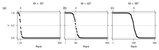
Figure 5: Rank-ordered eigenvalue spectrum including the eigenvalues $\eta_{m}$ of all $\mathsf{K}_{m}$, $-L\leq m\leq L$ for (a) $\Theta=30^{\circ}$, (b) $\Theta=60^{\circ}$, (c) $\Theta=90^{\circ}$, and $L=18$. The vertical gridlines mark the corresponding Shannon numbers $N$ of (85).

The eigenvalue spectrum of Slepian-type concentration problems [30, 28, 27] exhibits a characteristic step-like shape, and the present case is no exception. Figure 5 shows rank-ordered spectra including $\eta_{mn}$ for all orders $m$. They correspond to $\Theta=30^{\circ},60^{\circ},90^{\circ}$ and the maximal degree was chosen $L=18$.

The majority of the eigenvalues for each case is either close to one or zero, corresponding to well-concentrated and poorly concentrated eigenfunctions, respectively. As an illustration, in Fig. 6 we have plotted a small number of scalar eigenfunctions $G_{mn}$, corresponding to different parts of the eigenvalue spectrum.

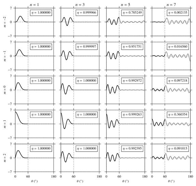
Figure 6: Four scalar eigenfunctions $G_{mn}(\cos\theta)$, $n=1,3,5,7$ of each order $-2\leq m\leq 2$. The maximal degree is $L=18$ and $\Theta=60^{\circ}$. The black and gray curves mark contributions of $G_{mn}$ to the interior of the spherical cap ($0\leq\theta\leq 60^{\circ}$) and the rest of the sphere ($60^{\circ}<\theta\leq 180^{\circ}$), respectively. Labels show the eigenvalues $\eta_{mn}$ which express the quality of concentration within $C$.

Strictly speaking, the solution of the concentration problem (56) is the pair of vectorial eigenfunctions which corresponds to the maximally concentrated $G_{m}$. However, having solved the equivalent eigenvalue problem (70), we have gained a whole set of well-concentrated, orthogonal pairs of eigenfunctions $\bm{\mathrm{G}}_{m}^{\pm}$. How many pairs belong to this set? To answer this question, we first define the partial Shannon number [26]

$$N_{m}:=\operatorname{Tr}\mathsf{K}_{m}=\sum_{n=1}^{L-\ell_{m}+1}\eta_{mn}=\int_{\cos\Theta}^{1}\mathcal{K}_{m}(x,x)\operatorname{d}\!x,$$ (84)

which gives the approximate number of reasonably well-concentrated ($\eta\geq 0.5$) scalar eigenfunctions for a given maximal degree $L$ and order $m$. Summing over all possible values of $m$, we obtain the (total) Shannon number

$$N:=\sum_{m=-L}^{L}N_{m}=\sum_{m=-L}^{L}\sum_{n=1}^{L-\ell_{m}+1}\eta_{mn}=\int_{\cos\Theta}^{1}\sum_{m=-L}^{L}\mathcal{K}_{m}(x,x)\operatorname{d}\!x=L(L+2)\frac{A_{C}}{4\pi},$$ (85)

where $A_{C}=2\pi(1-\cos\Theta)$ is the area of the spherical cap $C$. In the last equality we substituted definition (81), interchanged the order of double summation and used addition theorem (33).

Hence there are $N$ pairs of orthogonal vectorial eigenfunctions which are suitable for approximating bandlimited, tangential vector fields localized to $C$. Equivalently, the use of this basis reduces the number of degrees of freedom from $\dim S_{L}=2L(L+2)$ to $2N$.

3.3 Toward an efficient numerical solution: the commuting differential operator and its eigenvalue problem

In Section 3.1, we obtained the expansion coefficients $g_{lm}$ by solving eigenvalue equation (71) directly.However, while it is theoretically possible to calculate $g_{lm}$ this way, the accumulation of the eigenvalues $\eta$ at one and zero, as seen in Fig. 5, makes the numerical solution of (71) ill-conditioned [4]. In order to circumvent this problem, we set out to construct another matrix with a simple spectrum to supply the expansion coefficients $g_{lm}$.

Therefore, we first return to the Fredholm eigenvalue equation (80). We wish to find a Sturm–Liouville differential operator $\mathcal{J}_{m}$ that commutes with the concentration (integral) operator on the left-hand side of (80):

$$\int_{\cos\Theta}^{1}\mathcal{K}_{m}(x,x^{\prime})\mathcal{J}_{m}^{\prime}u(x^{\prime})\operatorname{d}\!x^{\prime}=\mathcal{J}_{m}\int_{\cos\Theta}^{1}\mathcal{K}_{m}(x,x^{\prime})u(x^{\prime})\operatorname{d}\!x^{\prime}=\int_{\cos\Theta}^{1}\mathcal{J}_{m}\mathcal{K}_{m}(x,x^{\prime})u(x^{\prime})\operatorname{d}\!x^{\prime}$$ (86)

for any square-integrable bandlimited function $u$, so that the two operators share a common set of eigenfunctions [3, pp. 314]. It is known from the Sturm–Liouville theory that $\mathcal{J}_{m}$ has a simple spectrum of distinct eigenvalues with an accumulation point in infinity [21, p. 724]. If such a differential operator $\mathcal{J}_{m}$ can be found, its matrix representation can be used to obtain the expansion coefficients $g_{lm}$ (hence the eigenfunctions) in a numerically stable way.

The same approach was taken by Grünbaum et al. for the concentration problem of scalar functions within $C$ [10]. They proposed the differential operator

$$\mathcal{G}_{m}:=(\cos\Theta-\cos\theta)\nabla_{\Omega,m}^{2}+\sin\theta\,\frac{\operatorname{d}\!}{\operatorname{d}\!\theta}-L(L+2)\cos\theta,$$ (87)

where $\nabla_{\Omega,m}^{2}$ is the fixed-order surface scalar Laplacian (41). This operator commutes with the concentration operator of the scalar case which contains the kernel function $\mathcal{D}_{m}(x,x^{\prime})=\sum_{l={\lvert m\rvert}}^{L}U_{lm}(x)U_{lm}(x^{\prime})$ [26].

Based on (87), we make the following ansatz on $\mathcal{J}_{m}$:

$$\mathcal{J}_{m}:=(\cos\Theta-\cos\theta)\Delta_{\Omega,m}+\sin\theta\frac{\operatorname{d}\!}{\operatorname{d}\!\theta}-L(L+2)\cos\theta,$$ (88)

where $\Delta_{\Omega,m}$ is the fixed-order operator (43) related to the surface vector Laplacian over $\Omega$. Changing the variable to $x=\cos\theta$ yields

$$\mathcal{J}_{m}=(\cos\Theta-x)\Delta_{\Omega,m}-(1-x^{2})\frac{\operatorname{d}\!}{\operatorname{d}\!x}-L(L+2)x,$$ (89)

which is equivalent to

$$\mathcal{J}_{m}=\frac{\operatorname{d}\!}{\operatorname{d}\!x}\left[(\cos\Theta-x)(1-x^{2})\frac{\operatorname{d}\!}{\operatorname{d}\!x}\right]-L(L+2)x-(\cos\Theta-x)\frac{m^{2}-2mx+1}{1-x^{2}}.$$ (90)

To prove that $\mathcal{J}_{m}$ satisfies the commutation relation (86), we suggest following the concept of Grünbaum et al. [10]. First, one proves the identity

$$\int_{\cos\Theta}^{1}u_{1}(x)\left[\mathcal{J}_{m}u_{2}(x)\right]\operatorname{d}\!x=\int_{\cos\Theta}^{1}\left[\mathcal{J}_{m}u_{1}(x)\right]u_{2}(x)\operatorname{d}\!x,$$ (91)

which holds for any two functions $u_{1}$ and $u_{2}$ that are non-singular at the interval endpoints (see A.7 for details). Therefore, the left-hand side of the commutation relation (86) can be rewritten as

$$\int_{\cos\Theta}^{1}\mathcal{K}_{m}(x,x^{\prime})\mathcal{J}_{m}^{\prime}u(x^{\prime})\operatorname{d}\!x^{\prime}=\int_{\cos\Theta}^{1}\left[\mathcal{J}_{m}^{\prime}\mathcal{K}_{m}(x,x^{\prime})\right]u(x^{\prime})\operatorname{d}\!x^{\prime}.$$ (92)

Finally, one verifies that

$$\mathcal{J}_{m}\mathcal{K}_{m}(x,x^{\prime})=\mathcal{J}_{m}^{\prime}\mathcal{K}_{m}(x,x^{\prime}).$$ (93)

The proof of (93), like the proof of (91), closely resembles its counterpart from the scalar concentration problem [26]. The key steps are the same, with the main difference that the associated Legendre functions are replaced by $F_{lm}$ together with the corresponding identities. The details can be found in A.8.

Since $\mathcal{J}_{m}$ commutes with the integral operator of (80), the functions $G_{m}$ are eigenfunctions of $\mathcal{J}_{m}$, too:

$$\mathcal{J}_{m}G_{m}(x)=\chi_{m}G_{m}(x).$$ (94)

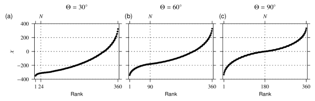
Figure 7: Rank-ordered eigenvalue spectrum including the eigenvalues $\chi_{m}$ of all $\mathsf{J}_{m}$, $-L\leq m\leq L$ for (a) $\Theta=30^{\circ}$, (b) $\Theta=60^{\circ}$, (c) $\Theta=90^{\circ}$, and $L=18$. The vertical gridlines mark the corresponding Shannon numbers $N=24,90,180$ (see (85)).

Figure 7 shows the $\chi$-eigenvalue spectrum of all orders $m$ for $\Theta=30^{\circ},60^{\circ},90^{\circ}$ and $L=18$ (cf. Fig. 5). Similarly to the scalar concentration problems [30, 28, 26], the rank-ordering for $\chi_{mn}$ is the opposite of the rank-ordering for $\eta_{mn}$. Importantly, the $\chi$-spectrum does not exhibit an accumulation of eigenvalues.

To obtain a matrix equation similar to the component-wise eigenvalue equation (78) of $\mathsf{K}_{m}$, we substitute expansion (75) of $G_{lm}$ in terms of $F_{lm}$ into eigenvalue equation (94), but this time, writing $l^{\prime}$ instead of $l$. After that we multiply by $F_{lm}(x)$, integrate over $-1\leq x\leq 1$, and invoke orthonormality relation (19) of $F_{lm}$. In this way, we arrive at the equation

$$\sum_{l^{\prime}=\ell_{m}}^{L}J_{m,ll^{\prime}}g_{l^{\prime}m}=\chi_{m}g_{lm},\quad\ell_{m}\leq l\leq L,$$ (95)

where

$$J_{m,ll^{\prime}}:=\int_{-1}^{1}F_{lm}(x)\mathcal{J}_{m}F_{l^{\prime}m}(x)\operatorname{d}\!x.$$ (96)

Similarly to $\mathsf{K}_{m}$, we can arrange $J_{m,ll^{\prime}}$ into a matrix $\mathsf{J}_{m}$:

$$\mathsf{J}_{m}=\begin{bmatrix}J_{m,\ell_{m}\ell_{m}}&\cdots&J_{m,\ell_{m}L}\\ \vdots&\ddots&\vdots\\ J_{m,L\ell_{m}}&\cdots&J_{m,LL}\end{bmatrix}.$$ (97)

However, the only non-zero matrix elements, as proven in A.9, are

$$J_{m,ll} =-l(l+1)\cos\Theta+m\left[1-\frac{L(L+2)+1}{l(l+1)}\right]$$ (98a)

$$J_{m,l,l+1} =J_{m,l+1,l}=\bigl{[}l(l+2)-L(L+2)\bigr{]}\zeta_{l+1,m},$$ (98b)

hence $\mathsf{J}_{m}$ is real, symmetric and tridiagonal. The eigenvalue equations (95) can thus be written as

$$\mathsf{J}_{m}\mathsf{g}_{m}=\chi_{m}\mathsf{g}_{m},\quad-L\leq m\leq L.$$ (99)

We have already seen in Section 2.2.1 that $F_{l,0}=U_{l,1}$, hence in the special case of $m=0$, matrix $\mathsf{J}_{0}$ is identical to the matrix of the Grünbaum operator $\mathcal{G}_{1}$ [26].

In summary, to calculate the scalar eigenfunctions $G_{m}$ for each order $m$, we first construct the tridiagonal matrices $\mathsf{J}_{m}$ using formulae (98) and then solve the corresponding eigenvalue problem (99) numerically. The resulting eigenvectors $\mathsf{g}_{m}$ contain the expansion coefficients $g_{lm}$, $\ell_{m}\leq l\leq L$, which, substituted into expansion (75) give the eigenfunctions $G_{m}$. The corresponding energy concentration ratio $\eta_{m}$ can be calculated using either $\eta_{m}=\int_{\cos\Theta}^{1}[G_{m}(x)]^{2}\operatorname{d}\!x$ or $\eta_{m}=\mathsf{g}_{m}^{\mathrm{T}}\mathsf{K}_{m}\mathsf{g}_{m}$.

Finally, we demonstrate the numerical stability of the proposed method. We calculated the eigenvectors $\mathsf{g}_{mn}$ for $m=1$, $L=18$ and $\Theta=30^{\circ},60^{\circ},90^{\circ}$ in multiple ways. First, as a reference, we used arbitrary precision arithmetic to obtain the eigenvectors of $\mathsf{K}_{1}$ with the relative error of each coefficient $g_{l,1}$ being less than $10^{-23}$. Let $\mathsf{g}_{1,n}^{\text{ref}}$ denote these vectors. Then we computed both $\mathsf{K}_{1}$ and $\mathsf{J}_{1}$ in double precision and fed them into the divide-and-conquer routines of LAPACK [2] to produce the eigenvectors again. Let $\mathsf{g}_{1,n}^{\text{K}}$ and $\mathsf{g}_{1,n}^{\text{J}}$ stand for these results, respectively. In addition, we furthermore assume ${\lVert\mathsf{g}_{1,n}^{\text{ref}}\rVert}={\lVert\mathsf{g}_{1,n}^{\text{K}}\rVert}={\lVert\mathsf{g}_{1,n}^{\text{J}}\rVert}=1$ where ${\lVert\mathsf{v}\rVert}:=\sqrt{\mathsf{v}^{\mathrm{T}}\mathsf{v}}$.

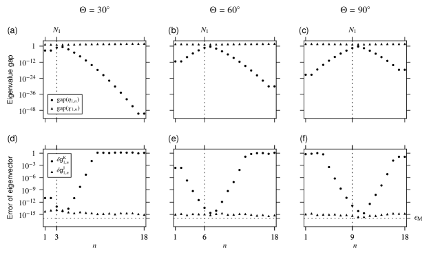
Figure 8: (a–c) Eigenvalue gap (100) for $\mathsf{K}_{1}$ (circle) and $\mathsf{J}_{1}$ (triangle) for $\Theta=30^{\circ},60^{\circ},90^{\circ}$, respectively. (d–f) Error (101) of the eigenvectors of $\mathsf{K}_{1}$ (circle) and $\mathsf{J}_{1}$ (triangle) for $\Theta=30^{\circ},60^{\circ},90^{\circ}$, respectively. The number $\epsilon_{\text{M}}$ denotes the machine epsilon in double precision. The maximal degree is $L=18$ and the vertical gridlines mark the partial Shannon numbers $N_{1}$ of (84).

Figures 8(a–c) plot the eigenvalue gaps [2, p. 104]

$$\operatorname{gap}\bigl{(}\eta_{1,n}\bigr{)} :=\min_{j\neq n}{\lvert\eta_{1,n}-\eta_{1,j}\rvert},$$ (100a)

$$\operatorname{gap}\bigl{(}\chi_{1,n}\bigr{)} :=\min_{j\neq n}{\lvert\chi_{1,n}-\chi_{1,j}\rvert},$$ (100b)

for all three values of $\Theta$, respectively, where $1\leq n\leq L$. Figures. 8(d–e) show the errors

$$\delta\mathsf{g}_{1,n}^{\text{K}} :=\min\left({\lVert\mathsf{g}_{1,n}^{\text{K}}-\mathsf{g}_{1,n}^{\text{ref}}\rVert},{\lVert\mathsf{g}_{1,n}^{\text{K}}-\bigl{(}-\mathsf{g}_{1,n}^{\text{ref}}\bigr{)}\rVert}\right),$$ (101a)

$$\delta\mathsf{g}_{1,n}^{\text{J}} :=\min\left({\lVert\mathsf{g}_{1,n}^{\text{J}}-\mathsf{g}_{1,n}^{\text{ref}}\rVert},{\lVert\mathsf{g}_{1,n}^{\text{J}}-\bigl{(}-\mathsf{g}_{1,n}^{\text{ref}}\bigr{)}\rVert}\right)$$ (101b)

of the eigenvectors, where we have taken their sign ambiguity into account.

In Figs. 8(a–c), we clearly see the accumulation of eigenvalues $\eta_{1,n}$ of $\mathsf{K}_{1}$ for both small and large values of $n$. The decrease in the eigenvalue gap by many orders of magnitude is accompanied by a rapid increase in the error $\delta\mathsf{g}_{1,n}^{\text{K}}$ [2, p. 104], as seen in Figs. 8(d–f). Therefore, with a naïve treatment of $\mathsf{K}_{1}$, we failed to calculate the well-concentrated eigenfunctions accurately; precisely those that play an important role in the approximation of functions localized to $C$.

On the contrary, Figs. 8(a–c) demonstrate again that the eigenvalues $\chi_{1,n}$ of $\mathsf{J}_{1}$ are well separated, hence we can expect the accuracy of eigenvectors $\mathsf{g}_{1,n}^{\text{J}}$ to stay reasonably close to machine precision. Indeed, the error is below $120\epsilon_{\text{M}}$ for all values of $n$, as indicated by Figs. 8(d–f), where $\epsilon_{\text{M}}=2^{-53}\approx 1.11\times 10^{-16}$ denotes the machine epsilon in double precision [2, p. 79]. Considering the tridiagonal form of $\mathsf{J}_{m}$ with the simple expressions (98) for the matrix elements, its superiority over $\mathsf{K}_{m}$ in the calculation of eigenvectors is justified.

4 Concluding remarks

We have formulated a scalar problem which is equivalent to the concentration problem of tangential vector fields within a spherical cap, and enables us to treat it analogously to the concentration problem of scalar functions. Hence a construction of a commuting differential operator with a simple spectrum has been made possible. This circumstance, at the same time, opens the way for computing concentrated vector fields in a fast and numerically stable way, as opposed to the direct method based on the ill-conditioned concentration matrix.

The reduction of the vector problem to an equivalent scalar one relies on a special combination of vector spherical harmonics, which we used as basis functions throughout this paper. With the help of the functions $F_{lm}$ of Sheppard and Török, for which we derived several novel relations, our mixed vector spherical harmonics can be expressed in a simple separable form. Finally, we note that these novel relations of $F_{lm}$ could facilitate the development of a fast vector spherical harmonic transform, too [33].

Appendix A Proofs

A.1 Proof of orthonormality relation (19)

Proof.

We first substitute definition (17) of $F_{lm}$ into the left-hand side of orthonormality relation (19). This yields

$$\begin{split}\int_{-1}^{1}F_{lm}(x)F_{l^{\prime}m}(x)\operatorname{d}\!x&=\frac{1}{l(l+1)}\int_{-1}^{1}\left[(1-x^{2})\frac{\operatorname{d}\!U_{lm}(x)}{\operatorname{d}\!x}\frac{\operatorname{d}\!U_{l^{\prime}m}(x)}{\operatorname{d}\!x}+\frac{m^{2}U_{lm}(x)U_{l^{\prime}m}(x)}{1-x^{2}}\right]\operatorname{d}\!x\\ &\quad-\frac{m}{l(l+1)}\int_{-1}^{1}\frac{\operatorname{d}\!}{\operatorname{d}\!x}\bigl{[}U_{lm}(x)U_{l^{\prime}m}(x)\bigr{]}\operatorname{d}\!x.\end{split}$$

The first term evaluates to [3, p. 754]

$$\frac{1}{l(l+1)}\int_{-1}^{1}\left[(1-x^{2})\frac{\operatorname{d}\!U_{lm}(x)}{\operatorname{d}\!x}\frac{\operatorname{d}\!U_{l^{\prime}m}(x)}{\operatorname{d}\!x}+\frac{m^{2}U_{lm}(x)U_{l^{\prime}m}(x)}{1-x^{2}}\right]\operatorname{d}\!x=\delta_{ll^{\prime}},$$

while for the second term, we get

$$\frac{m}{l(l+1)}\int_{-1}^{1}\frac{\operatorname{d}\!}{\operatorname{d}\!x}\bigl{[}U_{lm}(x)U_{l^{\prime}m}(x)\bigr{]}\operatorname{d}\!x=\frac{m}{l(l+1)}\bigl{[}U_{lm}(1)U_{l^{\prime}m}(1)-U_{lm}(-1)U_{l^{\prime}m}(-1)\bigr{]}=0,$$

where the last equality follows from the expression (14) for the values of $U_{lm}(\pm 1)$. Thus we end up with

$$\int_{-1}^{1}F_{lm}(x)F_{l^{\prime}m}(x)\operatorname{d}\!x=\delta_{ll^{\prime}}.\qed$$

A.2 Proof of recurrence relation (23)

Proof.

Using expressions (20) and (21) of $F_{lm}$ and recurrence relation (5) of $U_{lm}$, we transform the left-hand side (LHS) and right-hand side (RHS) separately so that only terms containing $U_{lm}$ and $U_{l-1,m}$ remain.

First we rewrite the LHS by inserting (20):

$$\begin{split}\text{LHS}&=\left[x-\frac{m}{l(l+1)}\right]F_{lm}(x)=\left[x-\frac{m}{l(l+1)}\right]\frac{-(lx+m)U_{lm}(x)+(2l+1)\xi_{lm}U_{l-1,m}(x)}{\sqrt{l(l+1)}\sqrt{1-x^{2}}}\\ &=-\frac{(lx+m)\bigl{[}l(l+1)x-m\bigr{]}}{\bigl{[}l(l+1)\bigr{]}^{3/2}\sqrt{1-x^{2}}}U_{lm}(x)+\frac{(2l+1)\bigl{[}l(l+1)x-m\bigr{]}}{\bigl{[}l(l+1)\bigr{]}^{3/2}\sqrt{1-x^{2}}}\xi_{lm}U_{l-1,m}(x).\end{split}$$

After that we proceed to the RHS. We insert (20) and (21), shifted in index $l$ by $+1$ and $-1$, respectively:

$$\begin{split}\text{RHS}&=\zeta_{l+1,m}F_{l+1,m}(x)+\zeta_{lm}F_{l-1,m}(x)\\ &=\zeta_{l+1,m}\frac{-\bigl{[}(l+1)x+m\big{]}U_{l+1,m}(x)+(2l+3)\xi_{l+1,m}U_{lm}(x)}{\sqrt{(l+1)(l+2)}\sqrt{1-x^{2}}}+\zeta_{lm}\frac{(lx-m)U_{l-1,m}(x)-(2l-1)\xi_{lm}U_{lm}(x)}{\sqrt{(l-1)l}\sqrt{1-x^{2}}}\end{split}$$

Next we expand $\zeta_{l+1,m}$ and $\zeta_{lm}$ using their definition (26). By straighforward, if lengthy, algebraic calculation, we get

$$\text{RHS}=\frac{-l^{2}\bigl{[}(l+1)x+m\big{]}\xi_{l+1,m}U_{l+1,m}(x)+(l+1)^{2}(lx-m)\xi_{lm}U_{l-1,m}(x)+m^{2}U_{lm}(x)}{\bigl{[}l(l+1)\bigr{]}^{3/2}\sqrt{1-x^{2}}}.$$

We apply recurrence relation (23) and collect like terms, hence

$$\begin{split}\text{RHS}&=\frac{-l^{2}x\bigl{[}(l+1)x+m\big{]}+m^{2}}{\bigl{[}l(l+1)\bigr{]}^{3/2}\sqrt{1-x^{2}}}U_{lm}(x)+\frac{l^{2}\bigl{[}(l+1)x+m\big{]}+(l+1)^{2}(lx-m)}{\bigl{[}l(l+1)\bigr{]}^{3/2}\sqrt{1-x^{2}}}\xi_{lm}U_{l-1,m}(x).\end{split}$$

Taking the difference $\text{LHS}-\text{RHS}$, it can be shown by further straightforward algebra that the coefficients of $U_{lm}$ and $U_{l-1,m}$ are zero. Hence $\text{LHS}=\text{RHS}$. ∎

A.3 Proof of recurrence relation (24)

Proof.

In this proof, we follow the same strategy as in the previous proof and rewrite the left-hand side (LHS) first. Inserting expression (20) of $F_{lm}$ yields

$$\text{LHS}=(1-x^{2})\frac{\operatorname{d}\!F_{lm}(x)}{\operatorname{d}\!x}=\frac{1}{\sqrt{l(l+1)}}(1-x^{2})\frac{\operatorname{d}\!}{\operatorname{d}\!x}\left[\frac{-(lx+m)U_{lm}(x)+(2l+1)\xi_{lm}U_{l-1,m}(x)}{\sqrt{1-x^{2}}}\right].$$

Performing the differentiation and using $(1-x^{2})\frac{\operatorname{d}\!}{\operatorname{d}\!x}(1-x^{2})^{-1/2}=x(1-x^{2})^{-1/2}$, we get

$$\begin{split}\text{LHS}=\Biggl{[}&-(lx+m)xU_{lm}(x)+(2l+1)\xi_{lm}xU_{l-1,m}(x)-l(1-x^{2})U_{lm}(x)-(lx+m)(1-x^{2})\frac{\operatorname{d}\!U_{lm}(x)}{\operatorname{d}\!x}\\ &+(2l+1)\xi_{lm}(1-x^{2})\frac{\operatorname{d}\!U_{l-1,m}(x)}{\operatorname{d}\!x}\Biggr{]}\times\bigl{[}l(l+1)(1-x^{2})\bigr{]}^{-1/2}.\end{split}$$

Next we insert recurrence relations (6) and (7), shifted in index $l$ by $+1$ and $-1$, respectively. After that we collect like terms and perform some straightforward algebra to obtain

$$\text{LHS}=\frac{(lx+m)(l-1)x-l(1-x^{2})-l^{2}+m^{2}}{\sqrt{l(l+1)}\sqrt{1-x^{2}}}U_{lm}(x)+\frac{(2l+1)(x-m)}{\sqrt{l(l+1)}\sqrt{1-x^{2}}}\xi_{lm}U_{l-1,m}(x).$$

Now we rewrite the right-hand side (RHS). We insert expressions (20) and (21) of $F_{lm}$, the second one shifted in index $l$ by $+1$.

$$\begin{split}\text{RHS}&=-l\left(x-\frac{m}{l^{2}}\right)F_{lm}(x)+(2l+1)\zeta_{lm}F_{l-1,m}(x)\\ &=\frac{(m/l-lx)\bigl{[}-(lx+m)U_{lm}(x)+(2l+1)\xi_{lm}U_{l-1,m}(x)\bigr{]}}{\sqrt{l(l+1)}\sqrt{1-x^{2}}}+\zeta_{lm}\frac{(2l+1)\bigl{[}(lx-m)U_{l-1,m}(x)-(2l-1)\xi_{lm}U_{lm}(x)\bigr{]}}{\sqrt{(l-1)l}\sqrt{1-x^{2}}}.\end{split}$$

Next we substitute definition (26) of $\zeta_{lm}$ and collect like terms. By straightforward algebra we get

$$\text{RHS}=\frac{(lx+m)(l^{2}x-m)-(l+1)(l^{2}-m^{2})}{l\sqrt{l(l+1)}\sqrt{1-x^{2}}}U_{lm}(x)+\frac{(2l+1)(x-m)}{\sqrt{l(l+1)}\sqrt{1-x^{2}}}\xi_{lm}U_{l-1,m}(x).$$

Taking the difference $\text{LHS}-\text{RHS}$, the terms containing $U_{l-1,m}$ cancel. It can be shown that the coefficient of $U_{lm}$ is zero as well, hence $\text{LHS}=\text{RHS}$. ∎

A.4 Proof of Christoffel–Darboux formula (27)

Proof.

We start from recurrence relation (23) and multiply both sides by $F_{lm}(x^{\prime})$. Then we take the same recurrence relation again, but this time, substitute $x^{\prime}$ for $x$ and multiply both sides by $F_{lm}(x)$. In this way, we obtain the following two equations:

$$\left[x-\frac{m}{l(l+1)}\right]F_{lm}(x)F_{lm}(x^{\prime}) =\zeta_{l+1,m}F_{l+1,m}(x)F_{lm}(x^{\prime})+\zeta_{lm}F_{l-1,m}(x)F_{lm}(x^{\prime}),$$

$$\left[x^{\prime}-\frac{m}{l(l+1)}\right]F_{lm}(x^{\prime})F_{lm}(x) =\zeta_{l+1,m}F_{l+1,m}(x^{\prime})F_{lm}(x)+\zeta_{lm}F_{l-1,m}(x^{\prime})F_{lm}(x).$$

Taking their difference and summing over $l$ yields

$$(x-x^{\prime})\sum_{l=\ell_{m}}^{L}F_{lm}(x)F_{lm}(x^{\prime})=\sum_{l=\ell_{m}}^{L} \Bigl{\{}\zeta_{l+1,m}\bigl{[}F_{l+1,m}(x)F_{lm}(x^{\prime})-F_{lm}(x)F_{l+1,m}(x^{\prime})\bigr{]}$$

$$+\zeta_{lm}\bigl{[}F_{l-1,m}(x)F_{lm}(x^{\prime})-F_{lm}(x)F_{l-1,m}(x^{\prime})\bigr{]}\Bigr{\}}.$$

We can see that consecutive terms cancel in the sum on the right-hand side. Moreover, $F_{\ell_{m}-1,m}=0$, thus only one term corresponding to $\zeta_{L+1,m}$ remains:

$$(x-x^{\prime})\sum_{l=\ell_{m}}^{L}F_{lm}(x)F_{lm}(x^{\prime})=\zeta_{L+1,m}\bigl{[}F_{L+1,m}(x)F_{Lm}(x^{\prime})-F_{Lm}(x)F_{L+1,m}(x^{\prime})\bigr{]}.\qed$$

A.5 Proof of $F_{lm}$ satisfying differential equation (28)

Proof.

First let us rearrange (28) and insert $F_{lm}$:

$$\frac{\operatorname{d}\!}{\operatorname{d}\!x}\left[(1-x^{2})\frac{\operatorname{d}\!F_{lm}(x)}{\operatorname{d}\!x}\right]=\left[-l(l+1)+\frac{m^{2}-2mx+1}{1-x^{2}}\right]F_{lm}(x).$$ (102)

The left-hand side can be transformed by exploiting recurrence relations (24) and (25) (the second one shifted in index $l$ by $-1$) as follows:

$$\frac{\operatorname{d}\!}{\operatorname{d}\!x}\left[(1-x^{2})\frac{\operatorname{d}\!F_{lm}(x)}{\operatorname{d}\!x}\right] =\frac{\operatorname{d}\!}{\operatorname{d}\!x}\left[-l\left(x-\frac{m}{l^{2}}\right)F_{lm}(x)+(2l+1)\zeta_{lm}F_{l-1,m}(x)\right]$$

$$=\biggl{[}-l^{2}(1-x^{2})F_{lm}(x)-(l^{2}x-m)(1-x^{2})\frac{\operatorname{d}\!F_{lm}(x)}{\operatorname{d}\!x}$$

$$\quad+l(2l+1)\zeta_{lm}(1-x^{2})\frac{\operatorname{d}\!F_{l-1,m}(x)}{\operatorname{d}\!x}\biggr{]}\times\bigl{[}l(1-x^{2})\bigr{]}^{-1}$$

$$=\biggl{\{}-l^{2}(1-x^{2})F_{lm}(x)-(l^{2}x-m)\left[-l\left(x-\frac{m}{l^{2}}\right)F_{lm}(x)+(2l+1)\zeta_{lm}F_{l-1,m}(x)\right]$$

$$\quad+l(2l+1)\zeta_{lm}\left[l\left(x-\frac{m}{l^{2}}\right)F_{l-1,m}(x)-(2l-1)\zeta_{lm}F_{lm}(x)\right]\biggr{\}}\times\bigl{[}l(1-x^{2})\bigr{]}^{-1}.$$

Collecting like terms yields

$$\begin{split}\frac{\operatorname{d}\!}{\operatorname{d}\!x}\left[(1-x^{2})\frac{\operatorname{d}\!F_{lm}(x)}{\operatorname{d}\!x}\right]=&\frac{-l^{2}(1-x^{2})+l(l^{2}x-m)(x-m/l^{2})-l(2l-1)(2l+1)\zeta_{lm}^{2}}{l(1-x^{2})}F_{lm}(x)\\ &+\frac{-(2l+1)(l^{2}x-m)+(2l+1)l^{2}(x-m/l^{2})}{l(1-x^{2})}\zeta_{lm}F_{l-1,m}(x).\end{split}$$

As expected, the term containing $F_{l-1,m}$ vanishes. Applying definition (26) of $\zeta_{lm}$ and expanding the fraction by $l$ yields

$$\frac{\operatorname{d}\!}{\operatorname{d}\!x}\left[(1-x^{2})\frac{\operatorname{d}\!F_{lm}(x)}{\operatorname{d}\!x}\right]=\frac{-l^{3}(1-x^{2})+(l^{2}x-m)^{2}-(l^{2}-1)(l^{2}-m^{2})}{l^{2}(1-x^{2})}F_{lm}(x).$$

By a straightforward, if lengthy, simplification we obtain

$$\frac{\operatorname{d}\!}{\operatorname{d}\!x}\left[(1-x^{2})\frac{\operatorname{d}\!F_{lm}(x)}{\operatorname{d}\!x}\right]=\left[-l(l+1)+\frac{m^{2}-2mx+1}{1-x^{2}}\right]F_{lm}(x).\qed$$

A.6 Proof of addition theorem (33)

Proof.

Upon inserting definition (17) of $F_{lm}$ into the left-hand side of addition theorem (33), we obtain

$$\begin{split}\sum_{m=-l}^{l}\bigl{[}F_{lm}(x)\bigr{]}^{2}&=\frac{1}{l(l+1)}\left\{\sum_{m=-l}^{l}(1-x^{2})\left[\frac{\operatorname{d}\!U_{lm}(x)}{\operatorname{d}\!x}\right]^{2}+\frac{1}{1-x^{2}}\sum_{m=-l}^{l}\bigl{[}U_{lm}(x)\bigr{]}^{2}\right\}\\ &\quad+\frac{2}{l(l+1)}\sum_{m=-l}^{l}m\frac{\operatorname{d}\!U_{lm}(x)}{\operatorname{d}\!x}U_{lm}(x).\end{split}$$

The first term yields $(2l+1)/2$ because of addition theorems (16), while the second term can be proven to vanish as follows:

$$\frac{2}{l(l+1)}\sum_{m=-l}^{l}m\frac{\operatorname{d}\!U_{lm}(x)}{\operatorname{d}\!x}U_{lm}(x) =\frac{2}{l(l+1)}\left[\sum_{m=-l}^{-1}m\frac{\operatorname{d}\!U_{lm}(x)}{\operatorname{d}\!x}U_{lm}(x)+\sum_{m=1}^{l}m\frac{\operatorname{d}\!U_{lm}(x)}{\operatorname{d}\!x}U_{lm}(x)\right]$$

$$=\frac{2}{l(l+1)}\sum_{m=1}^{l}\left[(-m)\frac{\operatorname{d}\!U_{l,-m}(x)}{\operatorname{d}\!x}U_{l,-m}(x)+m\frac{\operatorname{d}\!U_{lm}(x)}{\operatorname{d}\!x}U_{lm}(x)\right].$$

Using symmetry relation (12), we get

$$\frac{2}{l(l+1)}\sum_{m=-l}^{l}m\frac{\operatorname{d}\!U_{lm}(x)}{\operatorname{d}\!x}U_{lm}(x)=\frac{2}{l(l+1)}\sum_{m=1}^{l}\left[(-1)^{2m}(-m)+m\right]\frac{\operatorname{d}\!U_{lm}(x)}{\operatorname{d}\!x}U_{lm}(x),$$ (103)

hence

$$\frac{2}{l(l+1)}\sum_{m=-l}^{l}m\frac{\operatorname{d}\!U_{lm}(x)}{\operatorname{d}\!x}U_{lm}(x)=0.$$ (104)

Therefore,

$$\sum_{m=-l}^{l}\bigl{[}F_{lm}(x)\bigr{]}^{2}=\frac{2l+1}{2}.\qed$$

A.7 Proof of integral identity (91)

Proof.

Inserting expression (90) of $\mathcal{J}_{m}$ into both sides of integral identity (91) yields

$$\int_{\cos\Theta}^{1}u_{1}(x)\left[\mathcal{J}_{m}u_{2}(x)\right]\operatorname{d}\!x =\int_{\cos\Theta}^{1}u_{1}(x)\frac{\operatorname{d}\!}{\operatorname{d}\!x}\left[(\cos\Theta-x)(1-x^{2})\frac{\operatorname{d}\!u_{2}(x)}{\operatorname{d}\!x}\right]\operatorname{d}\!x$$

$$\quad+\int_{\cos\Theta}^{1}\left[L(L+2)u_{1}(x)u_{2}(x)-(\cos\Theta-x)\frac{m^{2}-2mx+1}{1-x^{2}}u_{1}(x)u_{2}(x)\right]\operatorname{d}\!x,$$ (105a)

$$\int_{\cos\Theta}^{1}\left[\mathcal{J}_{m}u_{1}(x)\right]u_{2}(x)\operatorname{d}\!x =\int_{\cos\Theta}^{1}\frac{\operatorname{d}\!}{\operatorname{d}\!x}\left[(\cos\Theta-x)(1-x^{2})\frac{\operatorname{d}\!u_{1}(x)}{\operatorname{d}\!x}\right]u_{2}(x)\operatorname{d}\!x$$

$$\quad+\int_{\cos\Theta}^{1}\left[L(L+2)u_{1}(x)u_{2}(x)-(\cos\Theta-x)\frac{m^{2}-2mx+1}{1-x^{2}}u_{1}(x)u_{2}(x)\right]\operatorname{d}\!x.$$ (105b)

Next we perform integration by parts on the first term of the right-hand side in both equations:

$$\int_{\cos\Theta}^{1}u_{1}(x)\frac{\operatorname{d}\!}{\operatorname{d}\!x}\left[(\cos\Theta-x)(1-x^{2})\frac{\operatorname{d}\!u_{2}(x)}{\operatorname{d}\!x}\right]\operatorname{d}\!x =u_{1}(x)(\cos\Theta-x)(1-x^{2})\frac{\operatorname{d}\!u_{2}(x)}{\operatorname{d}\!x}\,\bigg{|}_{\cos\Theta}^{1}$$

$$\quad-\int_{\cos\Theta}^{1}\frac{\operatorname{d}\!u_{1}(x)}{\operatorname{d}\!x}(\cos\Theta-x)(1-x^{2})\frac{\operatorname{d}\!u_{2}(x)}{\operatorname{d}\!x}\operatorname{d}\!x,$$

$$\int_{\cos\Theta}^{1}\frac{\operatorname{d}\!}{\operatorname{d}\!x}\left[(\cos\Theta-x)(1-x^{2})\frac{\operatorname{d}\!u_{1}(x)}{\operatorname{d}\!x}\right]u_{2}(x)\operatorname{d}\!x =(\cos\Theta-x)(1-x^{2})\frac{\operatorname{d}\!u_{1}(x)}{\operatorname{d}\!x}u_{2}(x)\,\bigg{|}_{\cos\Theta}^{1}$$

$$\quad-\int_{\cos\Theta}^{1}(\cos\Theta-x)(1-x^{2})\frac{\operatorname{d}\!u_{1}(x)}{\operatorname{d}\!x}\frac{\operatorname{d}\!u_{2}(x)}{\operatorname{d}\!x}\operatorname{d}\!x.$$

The first term on the right-hand side of both equations vanishes and the rest is identical, hence

$$\int_{\cos\Theta}^{1}u_{1}(x)\frac{\operatorname{d}\!}{\operatorname{d}\!x}\left[(\cos\Theta-x)(1-x^{2})\frac{\operatorname{d}\!u_{2}(x)}{\operatorname{d}\!x}\right]\operatorname{d}\!x=\int_{\cos\Theta}^{1}\frac{\operatorname{d}\!}{\operatorname{d}\!x}\left[(\cos\Theta-x)(1-x^{2})\frac{\operatorname{d}\!u_{1}(x)}{\operatorname{d}\!x}\right]u_{2}(x)\operatorname{d}\!x.$$ (106)

Upon inserting (106) into (105a) we find that

$$\int_{\cos\Theta}^{1}u_{1}(x)\left[\mathcal{J}_{m}u_{2}(x)\right]\operatorname{d}\!x=\int_{\cos\Theta}^{1}\left[\mathcal{J}_{m}u_{1}(x)\right]u_{2}(x)\operatorname{d}\!x.\qed$$

A.8 Proof of identity (93)

Proof.

First we apply expression (89) of $\mathcal{J}_{m}$ to the kernel function $\mathcal{K}_{m}(x,x^{\prime})$ and use eigenvalue equation (45) of $\Delta_{\Omega,m}$:

$$\mathcal{J}_{m}\mathcal{K}_{m}(x,x^{\prime}) =\left[(\cos\Theta-x)\Delta_{\Omega,m}-(1-x^{2})\frac{\operatorname{d}\!}{\operatorname{d}\!x}-L(L+2)x\right]\sum_{l=\ell_{m}}^{L}F_{lm}(x)F_{lm}(x^{\prime})$$

$$=-\cos\Theta\sum_{l=\ell_{m}}^{L}l(l+1)F_{lm}(x)F_{lm}(x^{\prime})+x\sum_{l=\ell_{m}}^{L}\bigl{[}l(l+1)-L(L+2)\bigr{]}F_{lm}(x)F_{lm}(x^{\prime})$$

$$\quad-(1-x^{2})\sum_{l=\ell_{m}}^{L}\frac{\operatorname{d}\!F_{lm}(x)}{\operatorname{d}\!x}F_{lm}(x^{\prime}).$$

Likewise, we also apply $\mathcal{J}_{m}^{\prime}$ to $\mathcal{K}(x,x^{\prime})$ and subtract the resulting equation from the previous one, yielding

$$(\mathcal{J}_{m}-\mathcal{J}_{m}^{\prime})\mathcal{K}_{m}(x,x^{\prime}) =(x-x^{\prime})\sum_{l=\ell_{m}}^{L}\bigl{[}l(l+1)-L(L+2)\bigr{]}F_{lm}(x)F_{lm}(x^{\prime})$$

$$\quad-\sum_{l=\ell_{m}}^{L}(1-x^{2})\frac{\operatorname{d}\!F_{lm}(x)}{\operatorname{d}\!x}F_{lm}(x^{\prime})$$

$$\quad+\sum_{l=\ell_{m}}^{L}F_{lm}(x)(1-x^{\prime\,2})\frac{\operatorname{d}\!F_{lm}(x^{\prime})}{\operatorname{d}\!x^{\prime}}.$$

Using recurrence relation (25) on the terms containing the derivatives of $F_{lm}$ and performing some straightforward algebra, we get

$$(\mathcal{J}_{m}-\mathcal{J}_{m}^{\prime})\mathcal{K}_{m}(x,x^{\prime}) =(x-x^{\prime})\sum_{l=\ell_{m}}^{L}\bigl{[}l^{2}-(L+1)^{2}\bigr{]}F_{lm}(x)F_{lm}(x^{\prime})$$

$$\quad+\sum_{l=\ell_{m}}^{L}(2l+1)\zeta_{l+1,m}\bigl{[}F_{l+1,m}(x)F_{lm}(x^{\prime})-F_{lm}(x)F_{l+1,m}(x^{\prime})\bigr{]}.$$

Applying Christoffel–Darboux formula (27) to the second term on the right-hand side yields

$$\begin{split}(\mathcal{J}_{m}-\mathcal{J}_{m}^{\prime})\mathcal{K}_{m}(x,x^{\prime})&=(x-x^{\prime})\sum_{l=\ell_{m}}^{L}F_{lm}(x)F_{lm}(x^{\prime})\bigl{[}l^{2}-(L+1)^{2}\bigr{]}\\ &\quad+(x-x^{\prime})\sum_{l=\ell_{m}}^{L}(2l+1)\sum_{l^{\prime}=\ell_{m}}^{l}F_{l^{\prime}m}(x)F_{l^{\prime}m}(x^{\prime}).\end{split}$$ (107)

In the last term of the right-hand side, the summation can be interchanged as

$$\sum_{l=\ell_{m}}^{L}(2l+1)\sum_{l^{\prime}=\ell_{m}}^{l}F_{l^{\prime}m}(x)F_{l^{\prime}m}(x^{\prime})=\sum_{l^{\prime}=\ell_{m}}^{L}F_{l^{\prime}m}(x)F_{l^{\prime}m}(x^{\prime})\sum_{l=l^{\prime}}^{L}(2l+1).$$

Relabeling the sums on the right-hand side of this expression, so that $l$ becomes $l^{\prime}$ and vice versa, and inserting the resulting expression into the right-hand side of (107), we obtain

$$(\mathcal{J}_{m}-\mathcal{J}_{m}^{\prime})\mathcal{K}_{m}(x,x^{\prime})=(x-x^{\prime})\sum_{l=\ell_{m}}^{L}F_{lm}(x)F_{lm}(x^{\prime})\left[l^{2}-(L+1)^{2}+\sum_{l^{\prime}=l}^{L}(2l^{\prime}+1)\right].$$

Since $\sum_{l^{\prime}=\ell_{m}}^{L}(2l^{\prime}+1)=(L+1)^{2}-l^{2}$, the right-hand side vanishes. Hence

$$\mathcal{J}_{m}\mathcal{K}_{m}(x,x^{\prime})=\mathcal{J}_{m}^{\prime}\mathcal{K}_{m}(x,x^{\prime}).\qed$$

A.9 Proof of expressions (98) for the matrix elements of $\mathcal{J}_{m}$

Proof.

We start by inserting expression (89) of $\mathcal{J}_{m}$ into the integral expression (96) for the matrix elements and use the eigenvalue equation (45) of $\Delta_{\Omega,m}$:

$$J_{m,ll^{\prime}} =\int_{-1}^{1}F_{lm}(x)\left[(\cos\Theta-x)\Delta_{\Omega,m}-(1-x^{2})\frac{\operatorname{d}\!}{\operatorname{d}\!x}-L(L+2)x\right]F_{l^{\prime}m}(x)\operatorname{d}\!x$$

$$=-l^{\prime}(l^{\prime}+1)\cos\Theta\int_{-1}^{1}F_{lm}(x)F_{l^{\prime}m}(x)\operatorname{d}\!x+\left[l^{\prime}(l^{\prime}+1)-L(L+2)\right]\int_{-1}^{1}xF_{lm}(x)F_{l^{\prime}m}(x)\operatorname{d}\!x$$

$$\quad-\int_{-1}^{1}F_{lm}(x)(1-x^{2})\frac{\operatorname{d}\!F_{l^{\prime}m}(x)}{\operatorname{d}\!x}\operatorname{d}\!x$$ (108)

The first integral is equal to $\delta_{ll^{\prime}}$ because of orthonormality relation (19). The remaining two can be evaluated by using recurrence relations (23) and (24) and orthonormality relation (19):

$$\int_{-1}^{1}xF_{lm}(x)F_{l^{\prime}m}(x)\operatorname{d}\!x =\zeta_{l^{\prime}m}\delta_{l,l^{\prime}-1}+\zeta_{l^{\prime}+1,m}\delta_{l,l^{\prime}+1}+\frac{m}{l^{\prime}(l^{\prime}+1)}\delta_{ll^{\prime}},$$

$$\int_{-1}^{1}F_{lm}(x)(1-x^{2})\frac{\operatorname{d}\!F_{l^{\prime}m}(x)}{\operatorname{d}\!x}\operatorname{d}\!x =(l^{\prime}+1)\zeta_{l^{\prime}m}\delta_{l,l^{\prime}-1}-l^{\prime}\zeta_{l^{\prime}+1,m}\delta_{l,l^{\prime}+1}+\frac{m}{l^{\prime}(l^{\prime}+1)}\delta_{ll^{\prime}}.$$

Thus for (108), we get

$$J_{m,ll^{\prime}}= \left\{-l^{\prime}(l^{\prime}+1)\cos\Theta+m\left[1-\frac{L(L+2)+1}{l^{\prime}(l^{\prime}+1)}\right]\right\}\delta_{ll^{\prime}}+\zeta_{l^{\prime}m}\left[(l^{\prime}-1)(l^{\prime}+1)-L(L+2)\right]\delta_{l,l^{\prime}-1}$$

$$+\zeta_{l^{\prime}+1,m}\left[l^{\prime}(l^{\prime}+2)-L(L+2)\right]\delta_{l^{\prime},l^{\prime}+1}.$$

Because of the Kronecker deltas, this expression is non-zero for index pairs $(l,l)$, $(l+1,l)$ and $(l,l+1)$ only. The corresponding matrix elements are

$$J_{m,ll} =-l(l+1)\cos\Theta+m\left[1-\frac{L(L+2)+1}{l(l+1)}\right]$$

$$J_{m,l,l+1} =J_{m,l+1,l}=\zeta_{l+1,m}\bigl{[}l(l+2)-L(L+2)\bigr{]},$$

hence $\mathsf{J}_{m}$ is real, symmetric and tridiagonal. ∎

References

- [1] Albertella, A., Sansò, F., Sneeuw, N.: Band-limited functions on a bounded spherical domain: the Slepian problem on the sphere. J. Geodesy 73(9), 436–447 (1999). DOI 10.1007/PL00003999
- [2] Anderson, E., Bai, Z., Bischof, C., Blackford, S., Demmel, J., Dongarra, J., Croz, J.D., Greenbaum, A., Hammarling, S., McKenney, A.: LAPACK Users’ Guide, third edn. Society for Industrial and Applied Mathematics, Philadelphia, PA (1999)
- [3] Arfken, G.B., Weber, H.J., Harris, F.E.: Mathematical Methods for Physicists: A Comprehensive Guide, 7th edn. Academic Press/Elsevier, Waltham, MA (2012)
- [4] Bell, B., Percival, D.B., Walden, A.T.: Calculating Thomson’s spectral multitapers by inverse iteration. J. Comput. Graph. Stat. 2(1), 119–130 (1993). DOI 10.1080/10618600.1993.10474602
- [5] Dahlen, F.A., Simons, F.J.: Spectral estimation on a sphere in geophysics and cosmology. Geophys. J. Int. 174(3), 774–807 (2008). DOI 10.1111/j.1365-246X.2008.03854.x
- [6] Das, S., Hajian, A., Spergel, D.N.: Efficient power spectrum estimation for high resolution CMB maps. Phys. Rev. D 79(8), 083,008 (2009). DOI 10.1103/PhysRevD.79.083008
- [7] Devaney, A.J., Wolf, E.: Multipole expansions and plane wave representations of the electromagnetic field. J. Math. Phys. 15(2), 234–244 (1974). DOI 10.1063/1.1666629
- [8] Eshagh, M.: Spatially restricted integrals in gradiometric boundary value problems. Artif. Satell. 44(4), 131–148 (2009). DOI 10.2478/v10018-009-0025-4
- [9] Gil, A., Segura, J., Temme, N.M.: Numerical Methods for Special Functions. Society for Industrial and Applied Mathematics, Philadelphia, PA (2007)
- [10] Grünbaum, F.A., Longhi, L., Perlstadt, M.: Differential operators commuting with finite convolution integral operators: some non-Abelian examples. SIAM J. Appl. Math. 42(5), 941–955 (1982). DOI 10.1137/0142067
- [11] Han, S.C., Ditmar, P.: Localized spectral analysis of global satellite gravity fields for recovering time-variable mass redistributions. J. Geod. 82(7), 423–430 (2008). DOI 10.1007/s00190-007-0194-5
- [12] Horn, R.A., Johnson, C.R.: Matrix analysis. Cambridge University Press, Cambridge, UK (1985). Reprinted with corrections 1990
- [13] Jahn, K., Bokor, N.: Vector Slepian basis functions with optimal energy concentration in high numerical aperture focusing. Opt. Commun. 285(8), 2028–2038 (2012). DOI 10.1016/j.optcom.2011.11.107
- [14] Landau, H.J., Pollak, H.O.: Prolate Spheroidal Wave Functions, Fourier Analysis and Uncertainty–II. Bell Syst. Tech. J. 40(1), 65–84 (1961)
- [15] Landau, H.J., Pollak, H.O.: Prolate Spheroidal Wave Functions, Fourier Analysis and Uncertainty–III: The Dimension of the Space of Essentially Time- and Band-limited Signals. Bell Syst. Tech. J. 41(4), 1295–1336 (1962)
- [16] Lessig, C., Fiume, E.: On the Effective Dimension of Light Transport 29(4), 1399–1403 (2010). DOI 10.1111/j.1467-8659.2010.01736.x
- [17] Liu, Q.H., Xun, D.M., Shan, L.: Raising and lowering operators for orbital angular momentum quantum numbers. Int. J. Theor. Phys. 49(9), 2164–2171 (2010). DOI 10.1007/s10773-010-0403-5
- [18] Maniar, H., Mitra, P.P.: The concentration problem for vector fields. Int. J. Bioelectromagn. 7(1), 142–145 (2005). URL http://www.ijbem.net/volume7/number1/pdf/037.pdf
- [19] Marinucci, D., Peccati, G.: Representations of SO(3) and angular polyspectra. J. Multivar. Anal. 101(1), 77–100 (2010). DOI 10.1016/j.jmva.2009.04.017
- [20] Moore, N.J., Alonso, M.A.: Closed-form bases for the description of monochromatic, strongly focused, electromagnetic fields. J. Opt. Soc. Am. A 26(10), 2211–2218 (2009). DOI 10.1364/JOSAA.26.002211
- [21] Morse, P.M., Feshbach, H.: Methods of Theoretical Physics, Part I. International Series in Pure and Applied Physics. McGraw-Hill, New York (1953)
- [22] Percival, D.B., Walden, A.T.: Spectral Analysis for Physical Applications: Multitaper and Conventional Univariate Techniques. Cambridge University Press, Cambridge, UK (1993). Reprinted with corrections 1998
- [23] Plattner, A., Simons, F.J.: Spatiospectral concentration of vector fields on a sphere. Appl. Comput. Harmon. Anal. (2013). DOI 10.1016/j.acha.2012.12.001. In press
- [24] Sheppard, C.J.R., Török, P.: Efficient calculation of electromagnetic diffraction in optical systems using a multipole expansion. J. Mod. Opt. 44(4), 803–818 (1997). DOI 10.1080/09500349708230696
- [25] Simons, F.J., Dahlen, F.A.: Spherical Slepian functions and the polar gap in geodesy. Geophys. J. Int. 166(3), 1039–1061 (2006). DOI 10.1111/j.1365-246X.2006.03065.x
- [26] Simons, F.J., Dahlen, F, .A., Wieczorek, M.A.: Spatiospectral concentration on a sphere. SIAM Rev. 48(3), 504–536 (2006). DOI 10.1137/S0036144504445765
- [27] Simons, F.J., Wang, D.V.: Spatiospectral concentration in the Cartesian plane. Int. J. Geomath. 2(1), 1–36 (2011). DOI 10.1007/s13137-011-0016-z
- [28] Slepian, D.: Prolate Spheroidal Wave Functions, Fourier Analysis and Uncertainty–IV: Extensions to Many Dimensions; Generalized Prolate Spheroidal Functions. Bell Syst. Tech. J. 43(6), 3009–3057 (1964)
- [29] Slepian, D.: Some comments on fourier analysis, uncertainty and modeling. SIAM Rev. 25(3), 379–393 (1983). DOI 10.1137/1025078
- [30] Slepian, D., Pollak, H.O.: Prolate Spheroidal Wave Functions, Fourier Analysis and Uncertainty–I. Bell Syst. Tech. J. 40(1), 43–63 (1961)
- [31] Swarztrauber, P.N.: The vector harmonic transform method for solving partial differential equations in spherical geometry. Mon. Weather Rev. 121(12), 3415–3437 (1993). DOI 10.1175/1520-0493(1993)121¡3415:TVHTMF¿2.0.CO;2
- [32] Szegő, G.: Orthogonal Polynomials, AMS Colloquium Publications, vol. 23, fourth edn. American Mathematical Society, Providence, RI (1975)
- [33] Tygert, M.: Recurrence relations and fast algorithms. Appl. Comput. Harmon. Anal. 28(1), 121–128 (2010). DOI 10.1016/j.acha.2009.07.005
- [34] Winch, D.E., Roberts, P.H.: Derivatives of addition theorems for Legendre functions. J. Aust. Math. Soc. B 37(2), 212–234 (1995). DOI 10.1017/S0334270000007670