Novel Features of the Transport Coefficients in Lifshitz Black Branes

Abstract

We study the transport coefficients, including the conductivities and shear viscosity of the non-relativistic field theory dual to the Lifshitz black brane with multiple $U(1)$ gauge fields by virtue of the gauge/gravity duality. Focusing on the case of double $U(1)$ gauge fields, we systematically investigate the electric, thermal and thermoelectric conductivities for the dual non-relativistic field theory. In the large frequency regime, we find a nontrivial power law behavior in the electric AC conductivity when the dynamical critical exponent $z>1$ in (2+1)-dimensional field theory. The relations between this novel feature and the ‘symmetric hopping model’ in condensed matter physics are discussed. In addition, we also show that the Kovtun-Starinets-Son bound for the shear viscosity to the entropy density is not violated by the additional $U(1)$ gauge fields and dilaton in the Lifshitz black brane.

I Introduction

The holographic principle 'tHooft:1993gx ; Susskind:1994vu , especially with its first realization in string theory-the AdS/CFT correspondence, offers us very intriguing and powerful tools to deal with the strongly coupled quantum systems from the dual viewpoint Maldacena:1997re ; Gubser:1998bc ; Witten:1998qj . The more general framework of the correspondence, which is called the gauge/gravity duality, has been extensively applied to the study of the QCD, Quark Gluon Plasma, hydrodynamics etc., for an incomplete list, see Witten:1998zw ; Rey:1998ik ; Maldacena:1998im ; Erlich:2005qh ; Policastro:2001yc ; Kovtun:2004de ; Brigante:2008gz ; Brigante:2007nu ; Policastro:2002se ; Kovtun:2003wp ; Son:2007vk ; Bhattacharyya:2008jc ; Bhattacharyya:2008kq ; Hansen:2008tq ; Iqbal:2008by ; Bredberg:2010ky ; Bredberg:2011jq ; Compere:2011dx ; Cai:2011xv ; Brattan:2011my ; Huang:2011he ; Niu:2011gu ; Eling:2011ct . In the frame work of the gauge/gravity duality, the features of strongly coupled quantum field theory on the conformally flat boundary can be fully captured by its dual weakly coupled classical gravitational or string theory in the curved bulk spacetime. Even though the gauge/gravity duality is widely believed to be held for arbitrary spacetime backgrounds, so far there are only a few explicit examples, in which the best known one is that the strongly coupled $\mathcal{N}=4$ supersymmetric Yang-Mills theory in four dimensional flat spacetime is equivalent to the classical (weakly coupled) limit of the type IIB superstring theory (supergravity) in AdS₅ $\times$ $S^{5}$ spacetime. For most other cases one still requires the bulk to be asymptotically AdS spacetime whereas the boundary field theory is conformally invariant and relativistic. However, besides numerous strongly coupled systems in high energy physics described by the relativistic quantum field theory, there also exist large classes of strongly coupled phenomena described by non-relativistic field theory in various condensed matter systems, especially near the (quantum) critical points. Therefore, it is very interesting and important to extend the gauge/gravity duality into a non-relativistic version in order to understand the strongly coupled phenomena in the laboratory condition.

Much progress has been made towards this direction in the past few years. One class of work focused on the study of field theories with the Schrödinger symmetry, motivated by the study of fermions at unitarity, see Son:2008ye ; Balasubramanian:2008dm . Another class of work tried to utilize the dual gravitational theories to study the condensed matter systems near quantum phase transitions that contain the Lifshitz fixed points Kachru:2008yh ; Kovtun:2008qy ; Taylor:2008tg ; Azeyanagi:2009pr ; McGreevy:2009xe ; Goldstein:2009cv ; Hartnoll:2009ns ; Cheng:2009df ; Lemos:2011gy ; Ross:2011gu ; Fang:2012pw , such as the strongly correlated electron systems. The particular property of the Lifshitz symmetry is that it consists of the anisotropic scaling

$$x\rightarrow\lambda x\quad{\rm and}\quad t\rightarrow\lambda^{z}t,$$ (1)

where $z$ is called the dynamical critical exponent. When $z=1$, the above transformation is the usual relativistic scaling. From the perspective of the gauge/gravity duality, the essential point is to construct bulk gravitational solutions by adding some appropriate sources to realize the boundary non-relativistic quantum field theories with the Lifshitz symmetry. The first attempt was done in Kachru:2008yh , in which a four dimensional asymptotic Lifshitz spacetime at zero temperature was obtained in the AdS Einstein gravity together with 1- and 2- form gauge fields. The bulk solution can be viewed as a toy model to provide us some useful descriptions for certain magnetic materials and liquid crystals. Subsequently, many asymptotic Lifshitz black hole solutions have been found and analyzed, see for example Taylor:2008tg ; Goldstein:2009cv ; Danielsson:2009gi ; Mann:2009yx ; Bertoldi:2009vn ; Cai:2009ac ; Pang:2009pd ; Bertoldi:2011zr . With the help of these solutions, important properties of the dual strongly coupled non-relativisitc quantum field theories, such as the transport coefficients, $n$-point correlation functions, renormalized stress tenosr and higher order corrections Keranen:2012mx ; Pang:2009wa ; Ross:2009ar ; Mann:2011hg , can be studied by performing the calculations on the side of the Lifshitz black holes/branes.

The asymptotic Lifshitz solutions can be obtained from different types of theories, the one received much attention is the Einstein-Maxwell-dilaton (EMD) theory, which can be used to model the dual non-relativistic quantum field theories at finite charge density . Recently, a class of analytic Lifshitz black hole/brane solutions have been solved in the EMD theory by adding multiple independent $U(1)$ gauge fields Tarrio:2011de . These kinds of charged Lifshitz black hole configurations can provide potential interesting applications to condensed matter systems such as fluids, non-Fermi liquids and conductors that contain the Lifshitz fixed points. Some holographic aspects in these spacetime backgrounds have been brought out, such as the instabilities of dual superfluid by adding probe charged scalar field in the bulk Mozaffar:2012bp . For other related works, see for example Tong:2012nf ; Alishahiha:2012qu ; Gursoy:2012ie .

The purpose of this paper is to utilize these charged Lifshitz black branes Tarrio:2011de to further study certain interesting phenomena of the dual strongly coupled non-relativistic quantum field theory with the Lifshitz fixed points on the boundary. Based on the dictionary of the gauge/gravity duality, we know that the multiple $U(1)$ gauge fields in the bulk will source multiple electric currents in the boundary field theory. As a theoretical model, there is no constraints on the number of independent electric currents even though their physical interpretations are not yet very clear. What we focus in this paper is to investigate the transport coefficients of the dual non-relativistic field theory, which includes the electric conductivity $\sigma$, the thermal conductivity $\bar{\kappa}$, the thermoelectric conductivity $\alpha$ and the shear viscosity $\eta$. To reach this goal, we consider the linearized gravitational and gauge fields perturbations (the scalar channel and the shear channel) in the bulk EMD theory. In particular, the bulk Lifshitz black hole can be viewed as the non-relativistic counterpart of the Reissner-Nordström-AdS black hole when $N=2$. Focusing on this case we calculate the conductivities of the dual non-relativistic field theories numerically, which are expected to capture the universal behavior of a class of conductors near the Lifshitz fixed points. Speicifically, after deriving the renormalized second order on-shell effective action, we work out the numerical results of conductivities, including the electric, thermoelectric and thermal conductivities. In particular, we work in $d=3$ and $d=4$ ($d$ is the dimension of the boundary field theory) for $1\leq z\leq 2$. We find some new frequency dependent power law features of the AC conductivities in the large frequency regime for $1<z\leq 2$. The possible relations between these novel features and the ‘symmetric hopping model’ in condensed matter physics are discussed in the context. In addition, an other interesting problem is to see whether these additional bulk $U(1)$ gauge fields and dilaton will affect the famous Kovtun-Starinents-Son (KSS) bound derived in the Einstein gravity Policastro:2001yc ; Kovtun:2004de . By solving the equation of motion of the transverse graviton at the low frequency limit and applying the linear response theory, we show that this bound is not violated although the additional gauge fields and dilaton do respectivley contribute to the shear viscosity as well as the entropy density of boundary charged fluids.

The outline of the paper is as follows. In Section II, we give a brief review of the Lifshitz black hole/brane backgrounds that we will use in this paper. In Section III, we obtain the renormalized second order on-shell action of the perturbations and compute the electric, thermal and thermoelectric conductivities of the boundary non-relativistic field theory, in the $N=2$ case. We calculate the shear viscosity of the boundary fluid both for $N=1$ and generic $N$ cases by solving the equation of motion of the transverse graviton in Section IV. Conclusions and discussions are drawn in Section V. Besides, we list some detailed calculations for deriving the perturbation equations and the second order on-shell actions in Appendix A.

II The configuration of Lifshitz black holes/branes

Let us consider the $(d+1)$ dimensional theory with action

$$I=\int{d^{d+1}x}\sqrt{-g}\left(R-\frac{\gamma(\phi)}{4}F^{2}-\frac{1}{2}(\partial\phi)^{2}-\frac{1}{2}J(\phi)A^{2}-V(\phi)\right),$$ (2)

where $F_{\mu\nu}=\partial_{\mu}A_{\nu}-\partial_{\nu}A_{\mu}$ is the $U(1)$ gauge field strength, $\phi$ is the dilaton field, $\gamma(\phi)$ is the coupling between the gauge field and the dilaton, $J(\phi)$ is the source term and $V(\phi)$ is the potential term. When we add $N\geq 1$ number of independent $U(1)$ gauge fields, the above variables can be accordingly changed as $\gamma(\phi)\rightarrow\sum^{N}_{a=1}\gamma_{a}(\phi)$ and $F_{\mu\nu}\rightarrow F_{a\mu\nu}$, and the equation of motions are

$$\Box\phi = \frac{dV(\phi)}{d\phi}+\frac{1}{4}\sum^{N}_{a=1}\frac{d\gamma_{a}}{d\phi}F^{2}_{a},$$

$$\nabla_{\mu}(f_{a}(\phi)F_{a}^{\mu\nu}) = JA_{a}^{\nu},$$

$$R_{\mu\nu}-\frac{1}{2}g_{\mu\nu}R = \frac{1}{2}\sum^{N}_{a=1}\gamma_{a}(\phi)\left(F_{a\mu\lambda}F_{a\nu}^{\lambda}-\frac{1}{4}g_{\mu\nu}F_{a}^{2}\right)+\frac{1}{2}J\left(A_{a\mu}A_{a\nu}-\frac{1}{2}A_{a}^{2}g_{\mu\nu}\right)$$ (3)

$$+\frac{1}{2}\left(\partial_{\mu}\phi\partial_{\nu}\phi-\frac{1}{2}g_{\mu\nu}(\partial\phi)^{2}-g_{\mu\nu}V(\phi)\right).$$

The Lifshitz black holes can be obtained from the following ansatz

$$ds^{2} = -\xi(r)e^{-\chi(r)}dt^{2}+\frac{dr^{2}}{\xi(r)}+b^{2}(r)dx^{i}dx_{i},$$ (4)

$$A_{a} = A_{at}(r)dt$$

together with

$$\quad\phi=\phi(r),\quad J(\phi)=0,\quad V(\phi)=2\Lambda\quad{\rm and}\quad\gamma_{a}=e^{\lambda_{a}\phi}.$$ (5)

Note that now the EPD model becomes the EMD model since we have set $J(\phi)=0$.

For $N=1$ case, the solution is

$$ds^{2}=-\frac{r^{2z}}{l^{2z}}\Xi(r)dt^{2}+\frac{l^{2}dr^{2}}{r^{2}\Xi(r)}+\frac{r^{2}}{l^{2}}\sum^{d-1}_{i=1}dx_{i}^{2},$$

$$\Xi(r)=1-\frac{r^{z+d-1}_{h}}{r^{z+d-1}},\quad A^{\prime}_{1t}=l^{-z}\sqrt{2(d+z-1)(z-1)}\mu^{\sqrt{\frac{d-1}{2(z-1)}}}r^{d+z-2},\quad e^{\phi}=\mu r^{\sqrt{2(z-1)(d-1)}},$$

$$\lambda=-\sqrt{\frac{2(d-1)}{z-1}},\quad\Lambda=-\frac{(z+d-2)(z+d-1)}{2l^{2}},$$ (6)

where $l$ is the curvature radius of the Lifshitz spacetime, $\mu$ is the scalar field amplitude, $m$ is related to the mass of the black hole and “^′” is the derivative with respect to $r$. The Hawking temperature and the Bekenstein-Hawking entropy are respectively

$$T=\frac{(z+d-1)r^{z}_{h}}{4\pi l^{z+1}},\quad S_{BH}=\frac{V_{d-1}}{4G_{d+1}}\left(\frac{r_{h}}{l}\right)^{d-1},$$ (7)

and $V_{d-1}=\int d^{d-1}x$ is the spatial volume of the boundary.

For generic $N$, the black hole solution is Tarrio:2011de

$$ds^{2}=-\frac{r^{2z}}{l^{2z}}f_{k}(r)dt^{2}+\frac{l^{2}}{r^{2}f_{k}(r)}dr^{2}+\frac{r^{2}}{l^{2}}d\Omega^{2}_{k,d-1},$$

$$f_{k}(r)=k(\frac{d-2}{d+z-3})^{2}\frac{l^{2}}{r^{2}}+1-mr^{-(d+z-1)}+\sum^{N-1}_{a=2}\frac{\rho^{2}_{a}\mu^{-\sqrt{2\frac{z-1}{d-1}}}l^{2z}}{2(d-1)(d+z-3)}r^{-2(d+z-2)},$$

$$A^{\prime}_{1t}=l^{-z}\sqrt{2(d+z-1)(z-1)}\mu^{\sqrt{\frac{d-1}{2(z-1)}}}r^{d+z-2},$$

$$A^{\prime}_{at}=\frac{\rho_{a}\mu^{-\sqrt{2\frac{z-1}{d-1}}}}{r^{d+z-2}},\quad(a=2,\ldots,N-1)$$

$$A^{\prime}_{Nt}=l^{1-z}\frac{\sqrt{2k(d-1)(d-2)(z-1)}}{\sqrt{d+z-3}}\mu^{\frac{d-2}{\sqrt{2(d-1)(z-{1})}}}r^{d+z-4},$$

$$\lambda_{1}=-\sqrt{\frac{2(d-1)}{z-1}},\quad\lambda_{a}=-\sqrt{\frac{2(z-1)}{d-1}},\quad\lambda_{N}=-\frac{d-2}{d-1}\sqrt{\frac{2(d-1)}{z-1}},\quad(a=2,\ldots,N-1),$$

$$e^{\phi}=\mu r^{\sqrt{2(d-1)(z-1)}},\quad\Lambda=-\frac{(d+z-1)(d+z-2)}{2l^{2}},$$ (8)

where $\rho_{a}$ are related to the charges of the black hole, while $k$ is the factor indicating the topology of the horizon. For $k=0$, the horizon is flat; for $k=-1$, the horizon is hyperbolic and the horizon is spherical for $k=1$. In the following, we shall take the spatial flat case, namely, the Lifshitz black brane with $k=0$. When $N\geq 2$, the black brane will contain multiple horizons in the presence of electromagnetic fields, let us define the outer event horizon to be located at $r=r_{h}$, i.e. $f(r_{h})=0$. Then the temperature of the black brane is

$$T=\frac{1}{4\pi}\left(\frac{r_{h}}{l}\right)^{z+1}f^{\prime}(r_{h})=\frac{1}{4\pi}\left(\frac{r_{h}}{l}\right)^{z+1}\left(\frac{2(d+z-2)}{r_{h}}-\frac{m(d+z-3)}{r_{h}^{d+z}}\right),$$ (9)

where $f(r)=1-mr^{-(d+z-1)}+\sum^{N-1}_{j=2}\frac{\rho^{2}_{j}\mu^{-\sqrt{2\frac{z-1}{d-1}}}l^{2z}}{2(d-1)(d+z-3)}r^{-2(d+z-2)}$. The horizon entropy $S_{BH}$ and entropy density $s$ of the dual CFT are

$$S_{BH}=\frac{r_{h}^{d-1}}{4G_{d+1}l^{d-1}}V_{d-1}\quad{\rm and}\quad s=\frac{S_{BH}}{V_{d-1}}=\frac{r_{h}^{d-1}}{4G_{d+1}l^{d-1}},$$ (10)

III The conductivities

In this section, we will compute the conductivities of the non-relativistic quantum field theory dual to the Lifshitz black brane. The electric conductivity $\sigma$ can be calculated by just turning on the bulk gauge field fluctuations $\delta A_{x}(t,r)=a_{x}(r)e^{-i\omega t}$. However, if we want to consider the thermal conductivity $\bar{\kappa}$ and the thermoelectric conductivity $\alpha$ , we need to consider the back reaction of the gauge fields to the metric, namely, we need to meanwhile turn on $\delta g_{tx}(t,r)=h_{tx}(r)e^{-i\omega t}$. For the EMD theory (when taking $J=0$) in eq.(2), we can obtain the linearized Einstein and Maxwell equations as (see Appendix A for details)

$$h^{\prime}_{tx}-\frac{2b^{\prime}}{b}h_{tx}+\sum_{a=1}^{N}\gamma_{a}(\phi)A^{\prime}_{at}a_{ax} = 0,$$ (11)

$$a^{\prime\prime}_{ax}+\left(\frac{(d-3)b^{\prime}}{b}+\frac{\xi^{\prime}}{\xi}-\frac{\chi^{\prime}}{2}+\frac{\phi^{\prime}}{\gamma_{a}(\phi)}\frac{d\gamma_{a}(\phi)}{d\phi}\right)a^{\prime}_{ax}+\frac{\omega^{2}}{\xi^{2}}e^{\chi}a_{ax} = \left(\frac{2b^{\prime}h_{tx}}{\xi b}-\frac{h^{\prime}_{tx}}{\xi}\right)A^{\prime}_{at}e^{\chi}.$$ (12)

where $b(r),\xi(r)$ and $\chi(r)$ are factors in eq.(4). Note that eq.(11) is the first order differential equation for $h_{tx}$ which can be integrated out as

$$h_{tx}=-b(r)^{2}\int\frac{1}{b(r)^{2}}\sum_{a=1}^{N}\gamma_{a}(\phi)A^{\prime}_{at}a_{ax}dr,$$ (13)

and eq.(12) can be written into the following equation as

$$a^{\prime\prime}_{ax}+\left(\frac{(d-3)b^{\prime}}{b}+\frac{\xi^{\prime}}{\xi}-\frac{\chi^{\prime}}{2}+\frac{\phi^{\prime}}{\gamma_{a}(\phi)}\frac{d\gamma_{a}(\phi)}{d\phi}\right)a^{\prime}_{ax}+\frac{\omega^{2}}{\xi^{2}}e^{\chi}a_{ax}=\frac{1}{\xi}\left(\sum_{c=1}^{N}\gamma_{c}(\phi)a_{cx}A^{\prime}_{ct}\right)A^{\prime}_{at}e^{\chi}$$ (14)

with the help of eq.(11).

When $N=1$, the background Lifshitz black brane eq.(II) is neutral as the Schwarzschild AdS black brane, the electric conductivity has been studied by adding a probe $U(1)$ gauge field in the bulk in Pang:2009wa .

In the following, we will focus on the $N=2$ situation, in which

$$e^{-\chi}=\left(\frac{r}{l}\right)^{2z-2},\quad\xi(r)=\frac{r^{2}}{l^{2}}f(r),\quad e^{\phi}=\mu r^{\sqrt{2(d-1)(z-1)}},\quad b(r)=\frac{r}{l},$$

$$f(r)=1-mr^{-(d+z-1)}+\frac{\rho^{2}_{2}\mu^{-\sqrt{2\frac{z-1}{d-1}}}l^{2z}}{2(d-1)(d+z-3)}r^{-2(d+z-2)}.$$ (15)

Recall that for the $N=2$ case, the background gauge field $A_{1t}$ is divergent at the spatial infinity, it only supports the asymptotic Lifshitz geometry instead of contributing to the free charge of the background electromagnetic field Tarrio:2011de . On the contrary, the gauge field $A_{2t}$ plays the role of the free electromagnetic field. Besides, our numeric results show that the asymptotic expansion of $a_{1x}$ is also divergent at the spatial infinity. Thus only the fluctuations of $A_{2}$, namely, $a_{2x}$ is the genuine electromagnetic perturbations, which will contribute to the electric conductivities of the dual field theory on the boundary. Consequently, to study the conductivities, we only need to turn on the perturbations $a_{2x}$ and $h_{tx}$, while turning off the perturbation $a_{1x}$. Then after substituting the above black brane solution eq.(III) into the original fluctuation equations (11) and (14), we obtain

$$h_{tx}^{\prime}-\frac{2}{r}h_{tx}+\rho_{2}r^{z-d}a_{2x} = 0,$$ (16)

$$a^{\prime\prime}_{2x}+\left(\frac{f^{\prime}}{f}+\frac{d+3z-4}{r}\right)a^{\prime}_{2x}+\left(\frac{\omega^{2}l^{2z+2}}{f^{2}r^{2z+2}}-\frac{\rho_{2}^{2}\mu^{-\sqrt{2\frac{z-1}{d-1}}}r^{(2-2d-2z)}l^{2z}}{f}\right)a_{2x} = 0.$$ (17)

The explicit asymptotic behavior of $a_{2x}$ near the infinite boundary with certain $d$ and $z$ considered in this paper can be found in Table 1, in which $C_{1}$ and $C_{2}$ are expansion coefficients that depend on the frequency $\omega$. According to the gauge/gravity duality, $C_{1}$ represents the source while $C_{2}$ represents the vacuum expectation value of the current operator $\mathfrak{J}_{x}$ dual to $a_{2x}$.

	$z=1$	$z=3/2$	$z=2$
$d=3$	$C_{1}+\frac{C_{2}}{r}$	$C_{1}+\frac{C_{2}}{r^{5/2}}$	$C_{1}+\frac{C_{1}\omega^{2}\log(r)}{4r^{4}}+\frac{C_{2}}{r^{4}}$
$d=4$	$C_{1}+\frac{C_{1}\omega^{2}\log(r)}{2r^{2}}+\frac{C_{2}}{r^{2}}$	$C_{1}+\frac{2C_{1}\omega^{2}}{3r^{3}}+\frac{C_{2}}{r^{7/2}}$	$C_{1}+\frac{C_{1}\omega^{2}}{4r^{4}}+\frac{C_{2}}{r^{5}}$

Table 1: The expansions of $a_{2x}$ with respect to various $d$ and $z$ near infinity. The coefficients $C_{1}$ and $C_{2}$ are functions of the frequency $\omega$.

In addition, the asymptotic behavior of $h_{tx}$ near the infinity boundary is,

$$h_{tx}\sim r^{2}h_{tx}^{(0)}+\frac{h_{tx}^{(1)}}{r^{(d-z-1)}}+\cdots,$$ (18)

where, $h_{tx}^{(1)}=C_{1}\rho_{2}/(1+d-z)$ in which $C_{1}$ is the source term of the expansions in $a_{2x}$, see Table 1.

III.1 Second order on-shell action

In order to compute the transport coefficients of $\sigma,\alpha$ and $\bar{\kappa}$, we need to know the quadratic on-shell actions for these perturbations. The on-shell action for the perturbation $a_{2x}$ and $h_{tx}$ up to 2nd order is (we have set $l=1$),

$$S^{(2)}_{\text{on-shell}}=S^{(2)}_{a_{2x}}+S^{(2)}_{h_{tx}},$$ (19)

where

$$S^{(2)}_{a_{2x}} = \int d^{d}x\bigg{(}-\frac{1}{2}a_{2x}a^{\prime}_{2x}e^{-\chi/2}\gamma_{2}(\phi)\xi r^{d-3}\bigg{)}\bigg{|}_{r\rightarrow\infty},$$ (20)

$$S^{(2)}_{h_{tx}} = \int d^{d}xe^{\chi/2}r^{d-3}\left(-h_{tx}h_{tx}^{\prime}+\frac{1}{2}h_{tx}^{2}(\frac{\xi^{\prime}}{\xi}-\chi^{\prime})\right)\bigg{|}_{r\rightarrow\infty}.$$ (21)

Usually the on-shell action eq.(19) is divergent near the asymptotic boundary, the divergence can be eliminated through the holographic renormalization approach, i.e. by adding appropriate boundary counter terms to the action (see, for example Balasubramanian:1999re ; Skenderis:2002wp ; Tarrio:2012xx ). In the configuration of the Lifshitz black brane, the counter terms have different forms with respect to different $d$ and $z$. We will list them in the following:

First of all, we will introduce the counter terms to $S^{(2)}_{a_{2x}}$ in eq.(20). These counter terms are classified according to the expansions of $a_{2x}$ in Table 1.

(a). $\mathbf{d=3,z=1~{}and~{}3/2}$:

In this case, the on-shell action of $S^{(2)}_{a_{2x}}$ is finite at the infinite boundary. There are no counter terms to $S^{(2)}_{a_{2x}}$ just like in the usual relativistic holographic superconductors Hartnoll:2008kx .

(b). $\mathbf{(d=3,z=2)~{}and~{}(d=4,z=1)}:$

For $(d=3,z=2)$ and $(d=4,z=1)$, there will be logarithmic divergence for $S^{(2)}_{a_{2x}}$ on the infinite boundary. In this case, the generic expansions of $a_{2x}$ near $r\rightarrow\infty$ now is,

$$a_{2x}(r)\sim C_{1}+\frac{C_{1}\omega^{2}\log(r)}{(d+3z-5)r^{d+3z-5}}+C_{2}\left(\frac{1}{r}\right)^{d+3z-5}.$$ (22)

The divergent term of $S^{(2)}_{a_{2x}}$ can be obtained from eq.(20) as,

$$I_{\text{div}.a_{2x}}=\frac{V_{d-1}}{T}{C_{1}}^{2}\omega^{2}\log(r)\mu^{\sqrt{2\frac{z-1}{d-1}}}$$ (23)

where $T$ is the temperature of the boundary field theory and $\frac{V_{d-1}}{T}$ is just the volume integration $\int dtd^{d-1}x_{i}$. Therefore, in this case the counter term should be,

$$I_{\text{ct}.a_{2x}}=-\frac{1}{2}\log(r)\int d^{d}x\sqrt{-\gamma^{0}}~{}\gamma_{2}(\phi)(F^{0}_{ij})^{2}.$$ (24)

where, $\gamma^{0}$ is the determinant of the induced metric while $F^{0}_{ij}$ is the induced gauge field strength on the asymptotic UV cut off boundary, respectively. It is easy to get that $(F^{0}_{ij})^{2}=2\omega^{2}(a_{2x})^{2}r^{-2z}/\xi$. Therefore, the finite on-shell $S^{(2)}_{a_{2x}}$ is,

$$I_{a_{2x}}^{(2)}=S^{(2)}_{a_{2x}}+I_{\text{ct}.a_{2x}}=\int d^{d}x~{}\left(C_{1}C_{2}(d+3z-5)-\frac{C_{1}^{2}\omega^{2}}{d+3z-5}\right).$$ (25)

(c). $\mathbf{d=4,z=3/2~{}and~{}2}$:

For $d=4$, $z=3/2$ and $z=2$, the general expansions of $a_{2x}$ is,

$$a_{2x}(r)\sim C_{1}+\frac{C_{1}\omega^{2}}{2(z-1)z}\left(\frac{1}{r}\right)^{2z}+C_{2}\left(\frac{1}{r}\right)^{3z-1}.$$ (26)

In this case, the divergent term of $S^{(2)}_{a_{2x}}$ is ,

$$I_{\text{div}.a_{2x}}=\frac{V_{d-1}}{T}\frac{\omega^{2}\mu^{\sqrt{2(z-1)/3}}C_{1}^{2}}{z-1}r^{z-1},$$ (27)

The counter term for this divergence now is,

$$I_{ct.a_{2x}}=\frac{-1}{2z-2}\int d^{d}x\sqrt{-\gamma^{0}}~{}\gamma_{2}(\phi)(F^{0}_{ij})^{2}.$$ (28)

Therefore, from the expansions, we can get the finite on-shell action as,

$$I_{a_{2x}}^{(2)}=S^{(2)}_{a_{2x}}+I_{ct.a_{2x}}=\int d^{d}x~{}C_{1}C_{2}(3z-1)\mu^{\sqrt{2(z-1)/3}}.$$ (29)

Next, we will introduce the counter terms for the on-shell action $S^{(2)}_{h_{tx}}$ in eq.(21). We can expand it near $r\rightarrow\infty$ as,

$$S^{(2)}_{h_{tx}}=I_{\text{div}.h_{tx}}+I_{\text{finite}.h_{tx}},$$ (30)

where,

$$I_{\text{div}.h_{tx}} = \int d^{d}x~{}(h_{tx}^{(0)})^{2}(z-2)r^{d-z+1},$$ (31)

$$I_{\text{finite}.h_{tx}} = \int d^{d}x~{}\left(\frac{(d+z-3)}{d-z+1}C_{1}\rho_{2}h_{tx}^{(0)}+\frac{1}{2}(h_{tx}^{(0)})^{2}m(d+z-1)r^{2-2z}\right).$$ (32)

It can be found that when $z=1$ the last term in $I_{\text{finite}.h_{tx}}$ is finite while for $z>1$ it will vanish at $r\rightarrow\infty$. As usual, we can introduce the Gibbons-Hawking term $I_{GH}$ and a counter term for the cosmological constant $I_{ct.cc}$ into the on-shell action to cancel the divergence, where

$$I_{GH} = 2\int d^{d}x\sqrt{-\gamma^{0}}K,$$ (33)

$$I_{ct.cc} = 2\int d^{d}x\sqrt{-\gamma^{0}}(d-1).$$ (34)

in which, $K=\gamma^{0}_{\mu\nu}\nabla^{\mu}n^{\nu}$ is the trace of the extrinsic curvature while $n^{\mu}$ is the outward pointing unit normal vector on the boundary. Expanding eq.(33) and eq.(34) to the quadratic order of the perturbations near $r\rightarrow\infty$, we arrive at,

$$I_{GH}^{(2)} = \int d^{d}x~{}\left((h_{tx}^{(0)})^{2}(z-d-1)r^{d-z+1}+\frac{1}{2}(h_{tx}^{(0)})^{2}m(d+z-1)r^{2-2z}\right),$$ (35)

$$I_{ct.cc}^{(2)} = \int d^{d}x~{}\left((h_{tx}^{(0)})^{2}(d-1)r^{d-z+1}+\frac{2(d-1)}{d-z+1}C_{1}\rho_{2}h_{tx}^{(0)}+\frac{1}{2}(h_{tx}^{(0)})^{2}(d-1)mr^{2-2z}\right).$$ (36)

Therefore, the total finite on-shell action of the perturbation $h_{tx}$ can be obtained from eqs.(31), (32), (35) and (36) as,

$$I_{h_{tx}}^{(2)} = S^{(2)}_{h_{tx}}-I_{GH}^{(2)}-I_{ct.cc}^{(2)}$$ (37)

$$= \int d^{d}x~{}\left(-C_{1}\rho_{2}h_{tx}^{(0)}-\frac{m(d-1)}{2}(h_{tx}^{(0)})^{2}r^{2-2z}\right)$$ (38)

$$= \int d^{d}x~{}\left(-(d+1-z)h_{tx}^{(0)}h_{tx}^{(1)}-\frac{m(d-1)}{2}(h_{tx}^{(0)})^{2}r^{2-2z}\right).$$ (39)

So, finally the total renormalized quadratic on-shell action for the perturbations $a_{2x}$ and $h_{tx}$ is,

$$I^{(2)}_{\text{total}}=I_{h_{tx}}^{(2)}=\int d^{d}x~{}\left(C_{1}C_{2}(d+3z-5)-(d+1-z)h_{tx}^{(0)}h_{tx}^{(1)}-\frac{m(d-1)}{2}(h_{tx}^{(0)})^{2}r^{2-2z}\right),$$ (40)

for $d=3,z=1~{}\text{and}~{}3/2$; Or,

$$I^{(2)}_{\text{total}} = I_{a_{2x}}^{(2)}+I_{h_{tx}}^{(2)}$$ (41)

$$= \int d^{d}x~{}\left(C_{1}C_{2}(d+3z-5)-\frac{C_{1}^{2}\omega^{2}}{d+3z-5}-(d+1-z)h_{tx}^{(0)}h_{tx}^{(1)}-\frac{m(d-1)}{2}(h_{tx}^{(0)})^{2}r^{2-2z}\right),~{}~{}~{}~{}~{}$$

when $(d=3,z=2)$ and $(d=4,z=1)$; Or,

$$I^{(2)}_{\text{total}} = I_{a_{2x}}^{(2)}+I_{h_{tx}}^{(2)}$$ (42)

$$= \int d^{d}x~{}\left(C_{1}C_{2}(3z-1)\mu^{\sqrt{2(z-1)/3}}-(d+1-z)h_{tx}^{(0)}h_{tx}^{(1)}-\frac{m(d-1)}{2}(h_{tx}^{(0)})^{2}r^{2-2z}\right).$$

when $d=4,z=3/2~{}\text{and}~{}2$.

III.2 The electric, thermoelectric and thermal conductivities

As long as we get the quadratic on-shell action for the perturbations, we can derive the electric and thermal transport coefficients jointly as follows:

$$\left(\begin{array}[]{c}{\langle}\mathfrak{J}_{x}{\rangle}\\ {\langle}Q_{x}{\rangle}\\ \end{array}\right)=\left(\begin{array}[]{cc}\sigma&\alpha T\\ \alpha T&\bar{\kappa}T\\ \end{array}\right)\left(\begin{array}[]{c}E_{x}\\ -(\nabla_{x}T)/T\\ \end{array}\right),$$ (49)

where $\mathfrak{J}_{x}$ is the electric current and $Q_{x}$ is the heat current, both are in the $x$-direction. And $\sigma,\alpha$ and $\bar{\kappa}$ are the electric conductivity, the thermoelectric conductivity and the thermal conductivity, respectively. Following the procedures in Hartnoll:2008kx ; Hartnoll:2009sz , we can obtain these transport coefficients which are listed in Table 2:

		$\sigma$	$\alpha$	$\bar{\kappa}$
$d=3$	$z=1$	$\frac{C_{2}(d+3z-5)}{i\omega C_{1}}$	$-\frac{\rho_{2}}{i\omega T}-\frac{\mu\sigma}{T}$	$-\frac{m(d-1)}{i\omega T}+\mu^{2}\sigma$
	$z=\frac{3}{2}$	$\frac{C_{2}(d+3z-5)}{i\omega C_{1}}$	$-\frac{\rho_{2}}{i\omega T}-\frac{\mu\sigma}{T}$	$\mu^{2}\sigma$
	$z=2$	$\frac{C_{2}(d+3z-5)}{i\omega C_{1}}-\frac{2\omega}{i(d+3z-5)}$	$-\frac{\rho_{2}}{i\omega T}-\frac{\mu\sigma}{T}$	$\mu^{2}\sigma$
$d=4$	$z=1$	$\frac{C_{2}(d+3z-5)}{i\omega C_{1}}-\frac{2\omega}{i(d+3z-5)}$	$-\frac{\rho_{2}}{i\omega T}-\frac{\mu\sigma}{T}$	$-\frac{m(d-1)}{i\omega T}+\mu^{2}\sigma$
	$z=\frac{3}{2}$	$\frac{C_{2}(3z-1)\mu^{\sqrt{2(z-1)/3}}}{i\omega C_{1}}$	$-\frac{\rho_{2}}{i\omega T}-\frac{\mu\sigma}{T}$	$\mu^{2}\sigma$
	$z=2$	$\frac{C_{2}(3z-1)\mu^{\sqrt{2(z-1)/3}}}{i\omega C_{1}}$	$-\frac{\rho_{2}}{i\omega T}-\frac{\mu\sigma}{T}$	$\mu^{2}\sigma$

Table 2: The various conductivities for different $z$ and $d$.

From Table 2, we can find that both of the thermoelectric conductivity $\alpha$ and the thermal conductivity depend on the electric conductivity $\sigma$ and the frequency $\omega$. Therefore, in Fig.1 and Fig.2 we only show the numerical results for the electric conductivity $\sigma$ since the rest transport coefficients can be easily obtained from $\sigma$. In the numerical calculations, we have scaled $l=1,r_{h}=1$, and $\rho_{2}=\mu=1$.

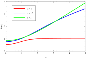
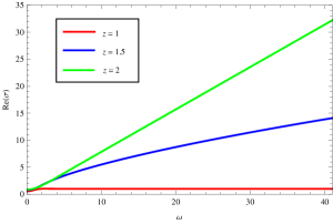
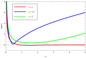
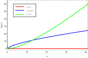
Figure 1: The real and imaginary parts of the conductivity for $d=3$ with respect to various $z$. The left parts are of the low frequency regime while the right parts are of the high frequency regime.

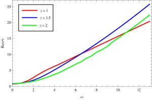
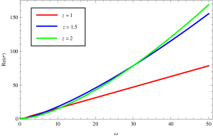
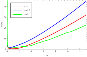
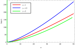
Figure 2: The real and imaginary parts of the conductivity for $d=4$ with respect to various $z$. The left parts are of the low frequency regime while the right parts are of the high frequency regime.

Actually, in the numerical calculations, we have set the integration starting point very close to the horizon but not exactly equal to $r_{h}$, because the coefficients of the eq.(17) will diverge at $r=r_{h}$, and we have adopted the usual incoming wave boundary conditions near the horizon. From Fig.1 and Fig.2, we can find that at $\omega=0$, the real parts of the conductivity is finite; however, the imaginary parts of the conductivity will diverge at $\omega=0$, thus from the Kramers-Kronig relations we can readily deduce that the real parts actually will develop a delta function at $\omega=0$. This delta function is due to the translational invariance of the system. These are known in previous literatures Hartnoll:2009sz .

For large frequencies, the expansions for $a_{2x}$ can be found in Table 1 in which the coefficients $C_{2}$ and $C_{1}$ are functions of $\omega$. Therefore, from Table 2 as well as Table 1, we can get the approximate behavior of the conductivity depending on the frequency $\omega$ as,

$$\sigma_{d=3}(\omega)\sim\left\{\begin{array}[]{cl}\omega^{0},&{z=1;}\\ \omega^{2/3},&{z=3/2;}\\ \omega(a+\log(\omega)),&{z=2.}\end{array}\right.\quad\sigma_{d=4}(\omega)\sim\left\{\begin{array}[]{cl}\omega(b+\log(\omega)),&{z=1;}\\ \omega^{4/3},&{z=3/2;}\\ \omega^{3/2},&{z=2.}\end{array}\right.$$ (56)

where, $a$ and $b$ are some constants. This large frequency behavior of the conductivities can be seen from the right parts of Fig. 1 and Fig. 2.

In Fig.1, the real part of the conductivity will tend to a constant when $\omega$ becomes large for $z=1$, which is similar to the previous papers Hartnoll:2008kx ; Hartnoll:2009sz . But the differences are in the case of $z=3/2$ and $z=2$, in which the Re($\sigma$) will depend on $\omega$ according to eq.(56). This is an interesting and new phenomenon from the viewpoint of the gauge/gravity duality, which is not observed before in the previous literatures as far as we know. For example, in Hartnoll:2009sz the author argued that the electric conductivity in the case of $d=3$ will tend to a constant because of the dimensional analysis. However, here we can explicitly see that in our model for $d=3$ and $z>1$, $\sigma$ will be proportional to $\omega^{s(z)}$ in the large frequency limit, where $s$ is a function of $z$. This peculiar frequency dependent AC electric conductivity may be related to some new materials in the realistic world. Fortunately, in Dyre:2000zz the author has studied the AC conductivity for various disordered solids in $(d=2+1)$ and $(d=3+1)$ dimensions both experimentally and theoretically. We found that the electric conductivity for $d=3$ and $d=4$ in our Fig.1 and Fig.2 have similar behaviors to the experiments or the computer simulations in the large frequency limit in the paper Dyre:2000zz . In that paper, the author has proposed a kind of ‘symmetric hopping model’ to illustrate the large frequency behavior of the electric conductivities. Therefore, we expect that the Lifshitz black brane model in the present paper may be related to this kind of ‘symmetric hopping model’ from certain aspects. We will further report this kind of relation in another work swz .

In Fig.2 for $z=1$, the large frequency behavior of the conductivity is like $\omega(b+\log(\omega))$, which resembles the expansions in the Appendix in Horowitz:2008bn . The arguments for the conductivity for $z=3/2$ and $z=2$ are the same as those for $d=3$ in Fig. 1.

IV The Shear viscosity

As we know that any interacting field theory at finite temperature in the limit of long time and long wavelength can be effectively described by hydrodynamics. In this section, we will compute the shear viscosity of the dual field theory in the low frequency limit. To do so, we need to turn on the transverse tensor mode fluctuation (which is the scalar channel) of the metric $\delta g_{\mu\nu}=h_{xy}$.

IV.1 The case of $N=1$

Let us begin with the $N=1$ case first, see eq.(II). Taking the mode expansion of the fluctuation $\delta g_{xy}(t,r)=h_{xy}(r)e^{-i\omega t+ik\zeta}$ (where $\zeta=x_{d-1}$, see the Appendix), we obtain the linearized Einstein equation of the $xy$ component as,

$$\varphi^{\prime\prime}+\left(\frac{z+d}{r}+\frac{\Xi^{\prime}}{\Xi}\right)\varphi^{\prime}+\left(\frac{l^{2+2z}\omega^{2}}{r^{2+2z}\Xi^{2}}-\frac{k^{2}l^{4}}{r^{4}\Xi}\right)\varphi=0.$$ (57)

which is the equation of motion of a minimally coupled massless scalar field propagating in the unperturbed spacetime background, where we have defined $\varphi=h^{x}_{y}$.

To solve eq.(57), it is convenient to introduce the new coordinate $u^{2}=\frac{r^{z+d-1}_{h}}{r^{z+d-1}}$, then the boundary is located at $u=0$, while $u=1$ is the horizon. After taking the long wavelength limit $k^{2}\rightarrow 0$, the fluctuation equation becomes

$$\varphi^{\prime\prime}+\left(\frac{\widetilde{\Xi}^{\prime}}{\widetilde{\Xi}}-\frac{1}{u}\right)\varphi^{\prime}+\frac{4l^{2(z+1)}\omega^{2}u^{\frac{2(z-d+1)}{d+z-1}}}{r^{2z}_{h}(z+d-1)^{2}\widetilde{\Xi}^{2}}\varphi=0.$$ (58)

where $\widetilde{\Xi}(u)=1-u^{2}$ and “^′” is the derivative with respect to $u$. At the horizon, since we are going to calculate the retarded Green’s function of the dual field theory, we need to impose the incoming wave boundary condition. Thus, we set $\varphi=(1-u)^{\alpha}\Psi(u)$, then $\alpha$ can be determined through the near horizon expansion of eq.(58), which gives $\alpha=-\frac{i\omega}{r^{z}_{h}(z+d-1)}$. To obtain the solution of $\Psi(u)$ in the full spacetime region, we can expand it in terms of $\omega$ as

$$\Psi(u)=\Psi_{0}(u)+\omega\Psi_{1}(u)+\mathcal{O}(\omega^{2}),$$ (59)

and then solve the above equation order by order. Furthermore, requiring $\Psi_{0}$ to be regular at the horizon and normalizing it to be one at the boundary, as well as $\Psi_{1}$ vanishes at the horizon, we find that

$$\Psi_{0}=1\quad{\rm and}\quad\Psi_{1}=-\frac{i}{(z+d-1)r^{z}_{h}}\ln(\frac{1+u}{2}),$$ (60)

then we have

$$\varphi=(1-u)^{-\frac{i\omega}{r^{z}_{h}(z+d-1)}}\left(1-\frac{i\omega}{(z+d-1)r^{z}_{h}}\ln(\frac{1+u}{2})\right).$$ (61)

To compute the shear viscosity of the boundary field theory, we need to compute the flux factor $\mathcal{F}=K\sqrt{-g}g^{uu}\varphi^{\ast}(u)\partial_{u}\varphi(u)$, where $K$ is a normalization constant related to the effective coupling constant of the bulk transverse graviton. Keeping to the order of $O(\omega)$, it is straightforward to compute the flux factor and the retarded 2-point Green’s function as

$$G_{R}=-2\mathcal{F}|_{u=0}=-\frac{i\omega r^{d-1}_{h}}{16\pi G_{d+1}l^{d-1}},$$ (62)

so the shear viscosity can be obtained by the Kubo formula as

$$\eta=-\lim_{\omega\rightarrow 0}\frac{{\rm Im}G_{R}(\omega,\vec{k}=0)}{\omega}=\frac{r^{d-1}_{h}}{16\pi G_{d+1}l^{d-1}},$$ (63)

then we have

$$\frac{\eta}{s}=\frac{1}{4\pi}$$ (64)

which satisfies the KSS bound in the Einstein gravity.

IV.2 The case of $N\geq 2$

Now we consider $N\geq 2$ cases, see eq.(II). As we have shown in the Appendix, the equation of motion for $\varphi=h^{x}_{y}$ is also that of a minimally coupled massless scalar field, which is of the same form as eq.(57)

$$\varphi^{\prime\prime}(r)+\left(\frac{f^{\prime}}{f}+\frac{d+z}{r}\right)\varphi^{\prime}(r)+\left(\frac{l^{2z+2}\omega^{2}}{r^{2z+2}f^{2}}-\frac{l^{4}k^{2}}{r^{4}f}\right)\varphi(r)=0.$$ (65)

Note that since $f(r)$ has multiple zero roots and cannot be determined in general, to solve eq.(65), it is more convenient to apply the matching method in which the exact form of $f(r)$ is not involved.

In the near horizon region, i.e. $r-r_{h}\ll r_{h}$, $f(r)\simeq f^{\prime}(r_{h})(r-r_{h})$, then eq.(65) can be simplified as

$$\varphi^{\prime\prime}(r)+\frac{1}{r-r_{h}}\varphi^{\prime}(u)+\left(\frac{c_{1}\omega^{2}}{(r-r_{h})^{2}}-\frac{c_{2}k^{2}}{r-r_{h}}\right)\varphi(r)=0,$$ (66)

in which

$$c_{1}=\left(\frac{1}{4\pi T}\right)^{2}\quad{\rm and}\quad c_{2}=\frac{1}{4\pi T}\left(\frac{r_{h}}{l}\right)^{z-3}.$$ (67)

Let’s further defining $\bar{r}=r/r_{h}$ and taking the long wavelength limit $k^{2}\rightarrow 0$, eq.(66) becomes

$$\varphi^{\prime\prime}(\bar{r})+\frac{1}{\bar{r}-1}\varphi^{\prime}(\bar{r})+\frac{c_{1}\omega^{2}}{(\bar{r}-1)^{2}}\varphi(\bar{r})=0,$$ (68)

which gives

$$\varphi(\bar{r})=\bar{c_{3}}(\bar{r}-1)^{\frac{i\mathfrak{w}}{2}}+\bar{c_{4}}(\bar{r}-1)^{\frac{-i\mathfrak{w}}{2}},$$ (69)

in the $r$ coordinate the solution is

$$\varphi(r)=c_{3}(r-r_{h})^{\frac{i\mathfrak{w}}{2}}+c_{4}(r-r_{h})^{\frac{-i\mathfrak{w}}{2}},$$ (70)

where $\mathfrak{w}=\frac{\omega}{2\pi T}$. The first part of (69) or (70) is the outgoing mode while the second part is the ingoing mode. To calculate the retarded Green’s function, we need to adopt the ingoing mode, which require $\bar{c_{3}}=c_{3}=0$ in eq.(69) and eq.(70). In the low frequency limit, eq.(70) can be expanded as

$$\varphi(r)=c_{4}\left(1-\frac{i\omega}{4\pi T}\ln(r-r_{h})+\mathcal{O}(\omega^{2})\right),$$ (71)

In the near region, $r_{h}\omega<r\omega\ll 1$, then in the $k^{2}\rightarrow 0$ limit, eq.(65) reduces to

$$\varphi^{\prime\prime}(r)+\left(\frac{f^{\prime}}{f}+\frac{d+z}{r}\right)\varphi^{\prime}(r)=0,$$ (72)

which can be solved as

$$\varphi(r)=\int\frac{c_{5}}{fr^{d+z}}dr+c_{6}.$$ (73)

Note that in the near horizon limit $r\rightarrow r_{h}$, eq.(73) can be simplified as

$$\varphi(r)\approx\int\frac{c_{5}}{f^{\prime}(r_{h})(r-r_{h})r_{h}^{d+z}}dr+c_{6}=\frac{c_{5}}{f^{\prime}(r_{h})r_{h}^{d+z}}\ln(r-r_{h})+c_{6}.$$ (74)

While in the large radius limit, $f(r)\rightarrow 1$, then eq.(73) becomes

$$\varphi(r)\approx\int\frac{c_{5}}{r^{d+z}}dr+c_{6}=-\frac{c_{5}}{(d+z-1)}\frac{1}{r^{d+z-1}}+c_{6},$$ (75)

In the outer region $r_{h}\ll l\ll r$, $f^{\prime}(r)\rightarrow 0$, $f(r)\rightarrow 1$ and again we taking $k^{2}\rightarrow 0$, then eq.(65) becomes

$$\varphi^{\prime\prime}(r)+\frac{d+z}{r}\varphi^{\prime}(r)+\frac{l^{2z+2}}{r^{2z+2}}\omega^{2}\varphi(r)=0,$$ (76)

in the $u={1}/{r}$ coordinate, eq.(76) can be changed to

$$\varphi^{\prime\prime}(u)-\frac{d+z-2}{u}\varphi^{\prime}(u)+l^{2z+2}u^{2z-2}\omega^{2}\varphi(u)=0,$$ (77)

ant its solution is

$$\varphi(u)=u^{\frac{\Delta_{+}}{2}}\left(c_{7}J_{-\frac{\Delta_{+}}{2z}}\left(\frac{l^{1+z}\omega u^{z}}{z}\right)+c_{8}J_{\frac{\Delta_{+}}{2z}}\left(\frac{l^{1+z}\omega u^{z}}{z}\right)\right),$$ (78)

where

$$c_{7}=\bar{c_{7}}(2z)^{-\frac{\Delta_{+}}{2z}}(l^{1+z}\omega)^{\frac{\Delta_{+}}{2z}}\Gamma\left(\frac{1-d+z}{2z}\right)\quad{\rm and}\quad c_{8}=\bar{c_{8}}(2z)^{-\frac{\Delta_{+}}{2z}}(l^{1+z}\omega)^{\frac{\Delta_{+}}{2z}}\Gamma\left(\frac{-1+d+3z}{2z}\right)$$

in which, $\bar{c}_{7}$ and $\bar{c}_{8}$ are certain constants while $\Delta_{+}=d+z-1$ is the conformal dimension of the operator dual to the massless scalar field in the bulk. Again, in the low frequency limit, eq.(78) can be expanded as

$$\varphi(r)=\bar{c_{7}}\left(1+\mathcal{O}(\omega^{2})\right)+\bar{c_{8}}l^{\frac{(1+z)\Delta_{+}}{z}}\left(\frac{2}{z}\right)^{\frac{\Delta_{+}}{z}}\omega^{1+\frac{d-1}{z}}r^{-\Delta_{+}}\left(1+\mathcal{O}(\omega^{2})\right).$$ (79)

The condition for matching the solutions in these three regions is $r_{h}<r\ll\omega^{-1}$. Comparing the eq.(74) with eq.(71) we get that

$$c_{4}=c_{6}\quad{\rm and}\quad-i\omega c_{4}=\frac{c_{5}}{l^{z+1}r_{h}^{d-1}}.$$ (80)

While the matching of eq.(75) with eq.(79) gives

$$c_{6}=\bar{c_{7}}\quad{\rm and}\quad-\frac{c_{5}}{d+z-1}=\bar{c_{8}}l^{\frac{(1+z)\Delta_{+}}{z}}\left(\frac{2}{z}\right)^{\frac{\Delta_{+}}{z}}\omega^{1+\frac{d-1}{z}}.$$ (81)

Namely, the coefficients in these three regions are related by the following relations

$$\bar{c_{7}}=c_{6}=c_{4}\quad{\rm and}\quad\bar{c_{8}}l^{\frac{(1+z)\Delta_{+}}{z}}\left(\frac{2}{z}\right)^{\frac{\Delta_{+}}{z}}\omega^{1+\frac{d-1}{z}}=c_{4}\frac{l^{z+1}r_{h}^{d-1}}{d+z-1}i\omega.$$ (82)

Furthermore, the normalization condition requires that $\varphi(r)$ is normalized to be $1$, namely, $c_{4}=1$. Consequently, the asymptotic solution at low frequency limit becomes

$$\varphi(r)=\left(r-r_{h}\right)^{\frac{-i{\mathfrak{w}}}{2}}\left(1+\frac{l^{z+1}r_{h}^{d-1}r^{-\Delta_{+}}}{(d+z-1)}i\omega+\mathcal{O}(\omega^{2})\right).$$ (83)

After eliminating the divergent terms, the dominant part of the radial flux of the scalar field at the boundary is

$$\mathcal{F} = K\sqrt{-g}g^{rr}\varphi^{*}(r)\partial_{r}\varphi(r)|_{r\rightarrow\infty}$$ (84)

$$= -iK\frac{r_{h}^{d-1}}{l^{d-1}}\omega+\mathcal{O}(\omega^{2})$$

$$= -\frac{i}{32\pi G_{d+1}}\frac{r_{h}^{d-1}}{l^{d-1}}\omega+\mathcal{O}(\omega^{2}),$$

where $K=1/(32\pi G_{d+1})$ is the effective coupling constant of the scalar field $\varphi(r)$, then the retarded Green’s function is

$$G_{R}(k)=-2\mathcal{F}(k,r)|_{r\rightarrow\infty},$$ (85)

and the shear viscosity is calculated from the Kubo formula

$$\eta = -\lim_{\omega\rightarrow 0}\frac{{\rm Im}G_{R}}{\omega}$$ (86)

$$= \frac{1}{16\pi G_{d+1}}\frac{r_{h}^{d-1}}{l^{d-1}},$$

Therefore, the ratio of the shear viscosity to the entropy is

$$\frac{\eta}{s}=\frac{1}{4\pi},$$ (87)

which gives the same value as that of the Lifshitz black brane with only one $U(1)$ gauge field. The result indicates that the additional background $U(1)$ gauge fields do not alter the KSS bound of the boundary fluid, though they do contribute to the shear viscosity and the entropy density, respectively.

V Conclusions and discussions

In this paper, we studied the model of strongly coupled non-relativistic quantum field theory with multiple $U(1)$ gauge fields near the Lifshitz fix points, in the frame work of the non-relativistic gauge/gravity duality. By considering the linearized perturbations of bulk gravitational and gauge fields, we solved the equation of motions for gauge fields with back reactions (shear channel) and the bulk transverse graviton (scalar channel). For the $N=2$ case, we derived the renormalized second order effective action and systematically calculated the electric, thermal and thermoelectric conductivities of the dual non-relativistic quantum field theories with respect to various $d$ and $z$. Specifically, we found the novel frequency dependent power law behavior of the AC electric conductivity in the large frequency limit when $d=3$ and $z>1$. From the knowledge of the condensed matter physics, we expect that our model provides a holographic description of the ‘symmetric hopping model’ in some sense. The argument goes to the case of $d=4$ as well, we will report the further relationship between the Lifshitz black brane and the hopping conductivities in another paper elsewhere. In addition, when taking the limit of long wavelength and low frequency in the generic $N$ cases, we also showed that the ratio of shear viscosity to entropy density of the dual boundary fluids still satisfies the KSS bound derived in the Einstein gravity.

Appendix A Linearized Perturbations of the Gravitational Theory

A.1 Einstein-Maxwell-dilaton theory

The Einstein-Maxwell-dilaton theory with multiple $U(1)$ gauge fields that we are considering has the action

$$I=\frac{1}{16\pi G_{d+1}}\int{d^{d+1}x}\sqrt{-g}\left(R-2\Lambda-\frac{1}{2}\partial^{\mu}\phi\partial_{\mu}\phi-\frac{1}{4}\sum^{N}_{a=1}e^{\lambda_{a}\phi}F^{2}_{a}\right),$$ (88)

its Einstein equation is

$$R_{\mu\nu}-\frac{2\Lambda}{d-1}g_{\mu\nu}=\frac{1}{2}\partial_{\mu}\phi\partial_{\nu}\phi+\frac{1}{2}\sum_{a=1}^{N}e^{\lambda_{a}\phi}\left(F_{a\lambda\mu}F_{a\nu}^{\lambda}-\frac{1}{2(d-1)}F_{a}^{2}g_{\mu\nu}\right).$$ (89)

Let us make the metric ansatz to be a $d+1$ dimensional black brane solution as

$$ds^{2}=H_{1}(r)\left(-f(r)dt^{2}+dx^{i}dx_{i}\right)+H_{2}(r)dr^{2},$$ (90)

where its outter horizon is located at $f(r_{h})=0$.

Consider the small metric fluctuation caused by some external perturbation

$$g^{(0)}_{\mu\nu}\rightarrow g_{\mu\nu}=g^{(0)}_{\mu\nu}+\delta g_{\mu\nu},$$ (91)

the Christoffel symbol is

$$\Gamma^{\lambda}_{\mu\nu} = \Gamma^{(0)\lambda}_{\mu\nu}+\delta\Gamma^{\lambda}_{\mu\nu}$$ (92)

$$= \Gamma^{(0)\lambda}_{\mu\nu}+\frac{g^{\lambda\alpha}}{2}\left(\nabla_{\mu}\delta g_{\alpha\nu}+\nabla_{\nu}\delta g_{\mu\alpha}-\nabla_{\alpha}\delta g_{\mu\nu}\right),$$

when taking the linear order perturbation of the metric, i.e. $\delta g_{\mu\nu}=h_{\mu\nu}$, the Christoffel symbol can be expanded up to second order of $h$ as

$$\Gamma^{\lambda}_{\mu\nu} = \Gamma^{(0)\lambda}_{\mu\nu}+\Gamma^{(1)\lambda}_{\mu\nu}+\Gamma^{(2)\lambda}_{\mu\nu},$$ (93)

where

$$\Gamma^{(1)\lambda}_{\mu\nu} = \frac{g^{(0)\lambda\alpha}}{2}\left(\nabla_{\mu}h_{\alpha\nu}+\nabla_{\nu}h_{\mu\alpha}-\nabla_{\alpha}h_{\mu\nu}\right),$$

$$\Gamma^{(2)\lambda}_{\mu\nu} = -\frac{h^{\lambda\alpha}}{2}\left(\nabla_{\mu}h_{\alpha\nu}+\nabla_{\nu}h_{\mu\alpha}-\nabla_{\alpha}h_{\mu\nu}\right).$$ (94)

Note that under the first order variation, the Ricci tensor varies as

$$R_{\mu\nu} = R^{(0)}_{\mu\nu}+\delta R^{(0)}_{\mu\nu}$$ (95)

$$= R^{(0)}_{\mu\nu}+R^{(1)}_{\mu\nu}+R^{(2)}_{\mu\nu},$$

where

$$R^{(1)}_{\mu\nu} = \Gamma^{(1)\alpha}_{\mu\nu;\alpha}-\Gamma^{(1)\alpha}_{\mu\alpha;\nu}$$ (96)

$$= \frac{1}{2}(\nabla^{\alpha}\nabla_{\mu}h_{\alpha\nu}+\nabla^{\alpha}\nabla_{\nu}h_{\alpha\mu})-\frac{1}{2}\Box h_{\mu\nu}-\frac{1}{2}\nabla_{\nu}\nabla_{\mu}h,$$

and

$$R^{(2)}_{\mu\nu} = \Gamma^{(2)\alpha}_{\mu\nu;\alpha}-\Gamma^{(2)\alpha}_{\mu\alpha;\nu}$$ (97)

$$= -\frac{h^{\alpha\beta}}{2}\left(\nabla_{\alpha}\nabla_{\mu}h_{\beta\nu}+\nabla_{\alpha}\nabla_{\nu}h_{\beta\mu}-\nabla_{\alpha}\nabla_{\beta}h_{\mu\nu}\right)+\frac{h^{\alpha\beta}}{2}\nabla_{\nu}\nabla_{\mu}h_{\alpha\beta}$$

$$-\frac{\nabla_{\alpha}h^{\alpha\beta}}{2}\left(\nabla_{\mu}h_{\beta\nu}+\nabla_{\nu}h_{\beta\mu}-\nabla_{\beta}h_{\mu\nu}\right)+\frac{\nabla_{\nu}h^{\alpha\beta}}{2}\nabla_{\mu}h_{\alpha\beta},$$

the first order and second order Ricci scalars are

$$R^{(1)} = g^{(0)\mu\nu}R^{(1)}_{\mu\nu}-h^{\mu\nu}R^{(0)}_{\mu\nu}$$ (98)

$$= \nabla^{\alpha}\nabla^{\beta}h_{\alpha\beta}-\Box h-\frac{2\Lambda}{d-1}h,$$

and

$$R^{(2)} = g^{(0)\mu\nu}R^{(2)}_{\mu\nu}-h^{\mu\nu}R^{(1)}_{\mu\nu}$$ (99)

$$= -h^{\mu\nu}\left(\nabla_{\mu}\nabla^{\lambda}h_{\nu\lambda}+\nabla^{\lambda}\nabla_{\mu}h_{\nu\lambda}\right)+h^{\mu\nu}\nabla_{\mu}\nabla_{\nu}h+h^{\mu\nu}\Box h_{\mu\nu}$$

$$-\nabla_{\alpha}h^{\alpha\lambda}\nabla^{\beta}h_{\beta\lambda}+\frac{\nabla_{\alpha}h^{\alpha\lambda}}{2}\nabla_{\lambda}h+\frac{\nabla_{\lambda}h^{\mu\nu}}{2}\nabla^{\lambda}h_{\mu\nu},$$

respectively.

Then the linearized Einstein equation is

$$R^{(1)}_{\mu\nu}-\frac{2\Lambda}{d-1}h_{\mu\nu}=\frac{1}{2}\sum_{a=1}^{N}e^{\lambda_{a}\phi}\left(-F_{a\alpha\mu}F_{a\beta\nu}h^{\alpha\beta}-\frac{1}{2(d-1)}(F_{a}^{2}h_{\mu\nu}-2F_{a\alpha}^{\gamma}F_{a\gamma\beta}h^{\alpha\beta}g^{(0)}_{\mu\nu})\right)$$ (100)

When there is only transverse gravitational fluctuation $h_{xy}=h_{xy}(r)e^{-i\omega t+ik\zeta}$, where $\zeta=x_{d-1}$ is the $d-1$-th spatial coordinate. Using the $R^{(0)x}_{x}$ component of the zeroth order eom, i.e.

$$R^{(0)x}_{x}-\frac{2\Lambda}{d-1}=\frac{1}{2}\sum_{a=1}^{N}e^{\lambda_{a}\phi}\left(-\frac{1}{2(d-1)}F_{a\lambda\alpha}F_{a\gamma\beta}g^{(0)\lambda\gamma}g^{(0)\alpha\beta}\right),$$

then eq.(100) becomes

$$-\frac{H_{1}}{2}\Box\varphi+\left(\frac{H_{1}^{{}^{\prime}2}}{2H_{1}H_{2}}-\frac{1}{2}\Box H_{1}\right)\varphi=\frac{2\Lambda}{d-1}H_{1}\varphi-\frac{1}{2}\sum_{a=1}^{N}e^{\lambda_{a}\phi}\frac{1}{2(d-1)}F_{a}^{2}H_{1}\varphi=R^{(0)}_{xx}\varphi$$ (101)

which gives the eom of minimally coupled massless scalar field $\varphi=h^{x}_{y}$

$$-\frac{H_{1}}{2}\Box\varphi=-\frac{H_{1}}{2}\frac{1}{\sqrt{-g^{(0)}}}\partial_{\mu}\left(\sqrt{-g^{(0)}}g^{(0)\mu\nu}\partial_{\nu}\varphi\right)=0.$$ (102)

A.2 Gauge field perturbation with back reaction

To compute the conductivities of the dual field theory, we need to turn on the gauge field perturbation along the spatial direction, this gauge field perturbation will in turn induce the $h_{ti}$ off-diagonal part of the background metric perturbation since $h_{ti}$ and $a_{ai}$ are the vector mode fluctuations. Without loss of generality, we choose $\delta A_{a\mu}=\delta^{\lambda}_{x}a_{a\lambda}(r)e^{-i\omega t+ik\zeta}$, which induces the corresponding metric perturbation is $\delta g_{\mu\nu}=h_{tx}(r)e^{-i\omega t+ik\zeta}$. Then the linearized Einstein and Maxwell equations are obtained by making the combined diffeomorphism and gauge variations to the original equations, namely

$$\delta_{\epsilon+\chi}\left(R_{\mu\nu}-\frac{2\Lambda}{d-1}g_{\mu\nu}\right)=\delta_{\epsilon+\chi}\left(\frac{1}{2}\partial_{\mu}\phi\partial_{\nu}\phi+\frac{1}{2}\sum_{a=1}^{N}e^{\lambda_{a}\phi}\left(F_{a\lambda\mu}F_{a\nu}^{\lambda}-\frac{1}{2(d-1)}F_{a}^{2}g_{\mu\nu}\right)\right),$$ (103)

where $\delta_{\epsilon}$ means the diffeomorphism transformation while $\delta_{\chi}$ indicates the gauge field transformation that obeying the following relations

$$\delta_{\epsilon}g_{\mu\nu}=\mathcal{L}_{\epsilon}g_{\mu\nu}\quad{\rm and}\quad\delta_{\chi}A_{a\mu}=a_{a\mu}.$$ (104)

In the linear order perturbation, the nonvanishing components of the first order Ricci tensor are $R_{xt}=R_{tx}$ and $R_{xr}=R_{rx}$. Then the linearized Einstein equation are

$$R^{(1)}_{xt}-\frac{2\Lambda}{d-1}h_{xt} = \frac{1}{2}\sum_{a=1}^{N}e^{\lambda_{a}\phi}\left(g^{(0)rr}\partial_{r}a_{ax}\partial_{r}A_{at}-\frac{1}{2(d-1)}F^{(0)2}_{a}h_{xt}\right),$$ (105)

together with the $xx$ component of the zeroth order Einstein equation, eq.(105) becomes

$$\frac{1}{4fH_{1}H_{2}^{2}}\left(H_{2}f^{\prime}(h_{tx}^{\prime}H_{1}-h_{tx}H_{1}^{\prime})+fH_{1}(h_{tx}^{\prime}H_{2}^{\prime}-2h_{tx}^{\prime\prime}H_{2})+fh_{tx}(-H_{1}^{\prime}H_{2}^{\prime}+2H_{1}^{\prime\prime}H_{2})\right)$$

$$=\frac{1}{2H_{2}}\sum_{a=1}^{N}e^{\lambda_{a}\phi}a_{ax}^{\prime}A_{at}^{\prime},$$ (106)

and

$$R^{(1)}_{rt} = -\frac{1}{2}\sum_{a=1}^{N}e^{\lambda_{a}\phi}g^{(0)tt}\partial_{t}a_{ax}A_{at}^{\prime}=\frac{i\omega}{2}\sum_{a=1}^{N}e^{\lambda_{a}\phi}g^{(0)tt}a_{ax}A_{at}^{\prime},$$ (107)

which gives

$$h^{\prime}_{tx}-\frac{H_{1}^{\prime}}{H_{1}}h_{tx}+\sum_{a=1}^{N}e^{\lambda_{a}\phi}a_{ax}A^{\prime}_{at}=0,$$ (108)

where “^′” indicates $\partial_{r}$.

In addition, the linearized Maxwell equation is obtained by

$$\delta_{\epsilon+\chi}\partial_{\mu}\left(\sqrt{-g}e^{\lambda_{a}\phi}g^{\mu\alpha}g^{\nu\beta}F_{a\alpha\beta}\right)$$ (109)

$$= \partial_{\mu}\left(\frac{\sqrt{-g^{(0)}}}{2}e^{\lambda_{a}\phi}g^{(0)\rho\sigma}h_{\rho\sigma}g^{(0)\mu\alpha}g^{(0)\nu\beta}F^{(0)}_{a\alpha\beta}\right)$$

$$-\partial_{\mu}\left(\sqrt{-g^{(0)}}e^{\lambda_{a}\phi}(h^{\mu\alpha}g^{(0)\nu\beta}+g^{(0)\mu\alpha}h^{\nu\beta})F^{(0)}_{a\alpha\beta}\right)$$

$$+\partial_{\mu}\left(\sqrt{-g^{(0)}}e^{\lambda_{a}\phi}g^{(0)\mu\alpha}g^{(0)\nu\beta}(\partial_{\alpha}a_{a\beta}-\partial_{\beta}a_{a\alpha})\right)=0,$$

its nonvanishing components are

$$\partial_{r}\left(\sqrt{-g}e^{\lambda_{a}\phi}g^{(0)rr}g^{(0)xx}g^{(0)tt}(-h_{tx})\partial_{r}A_{at}\right) + \partial_{t}\left(\sqrt{-g}e^{\lambda_{a}\phi}g^{(0)xx}g^{(0)tt}\partial_{t}a_{ax}\right)$$

$$+ \partial_{r}\left(\sqrt{-g}e^{\lambda_{a}\phi}g^{(0)rr}g^{(0)xx}\partial_{r}a_{ax}\right)=0.$$

In the black brane background eq.(90), the above equations become

$$a^{\prime\prime}_{ax}+\left(\frac{(d-2)H^{\prime}_{1}}{2H_{1}}-\frac{H^{\prime}_{2}}{2H_{2}}+\frac{f^{\prime}}{2f}+\lambda_{a}\phi^{\prime}\right)a^{\prime}_{ax}+\frac{\omega^{2}H_{2}}{fH_{1}}a_{ax}=\left(\frac{H^{\prime}_{1}h_{tx}}{fH_{1}^{2}}-\frac{h^{\prime}_{tx}}{fH_{1}}\right)A^{\prime}_{at}.$$ (110)

When taking the ansatz $H_{1}=b^{2}$, $H_{2}=1/\xi$, $f(r)=\xi e^{-\chi}/b^{2}$ and $\gamma_{a}(\phi)=e^{\lambda_{a}\phi}$ in eq.(4), eq.(108) and eq.(110) change into

$$h^{\prime}_{tx}-\frac{2b^{\prime}}{b}h_{tx}+\sum_{a=1}^{N}\gamma_{a}(\phi)A^{\prime}_{at}a_{ax}=0,$$ (111)

and

$$a^{\prime\prime}_{ax}+\left(\frac{(d-3)b^{\prime}}{b}+\frac{\xi^{\prime}}{\xi}-\frac{\chi^{\prime}}{2}+\frac{\phi^{\prime}}{\gamma_{a}(\phi)}\frac{d\gamma_{a}(\phi)}{d\phi}\right)a^{\prime}_{ax}+\frac{\omega^{2}}{\xi^{2}}e^{\chi}a_{ax}=\left(\frac{2b^{\prime}h_{tx}}{\xi b}-\frac{h^{\prime}_{tx}}{\xi}\right)A^{\prime}_{at}e^{\chi}.$$ (112)

In the linear order perturbation of the metric and the gauge fields, the bulk action can also be expanded into second order as

$$I = I^{(0)}+I^{(1)}+I^{(2)},$$ (113)

where the zeroth order action is

$$I^{(0)} = \frac{1}{16\pi G_{d+1}}\int{d^{d+1}x}\sqrt{-g^{(0)}}\left(R^{(0)}-2\Lambda-\frac{1}{2}g^{(0)\mu\nu}\partial_{\mu}\phi\partial_{\nu}\phi-\frac{1}{4}\sum^{N}_{a=1}e^{\lambda_{a}\phi}F^{(0)2}_{a}\right)$$ (114)

$$= \frac{1}{16\pi G_{d+1}}\int{d^{d+1}x}\sqrt{-g^{(0)}}\left(\frac{4\Lambda}{d-1}-\frac{1}{2(d-1)}\sum^{N}_{a=1}e^{\lambda_{a}\phi}F^{(0)2}_{a}\right),$$

and the first order action is

$$I^{(1)} = \frac{1}{16\pi G_{d+1}}\int{d^{d+1}x}\sqrt{-g^{(0)}}\left(\nabla^{\mu}\nabla^{\nu}h_{\mu\nu}-\Box h-\frac{1}{2}\sum^{N}_{a=1}e^{\lambda_{a}\phi}F^{(0)}_{a\mu\nu}F^{(1)\mu\nu}_{a}\right)$$ (115)

$$= \frac{1}{16\pi G_{d+1}}\int_{\Sigma}{d^{d}x}\sqrt{-g^{(0)}}n_{\mu}\left(\nabla^{\nu}h^{\mu}_{\nu}-\nabla^{\mu}h-\sum^{N}_{a=1}a_{a\nu}\left(e^{\lambda_{a}\phi}F^{(0)\mu\nu}_{a}\right)\right),$$

which are purely surface terms when the bulk eoms are satisfied (on-shell condition), where $n_{\mu}$ is the unit normal vector of the hypersurface $\Sigma$.

While the second order action is

$$I^{(2)} = \frac{1}{16\pi G_{d+1}}\int{d^{d+1}x}\sqrt{-g^{(0)}}\{-h^{\mu\nu}\nabla^{\lambda}\nabla_{\mu}h_{\nu\lambda}+\frac{1}{2}h^{\mu\nu}\nabla_{\mu}\nabla_{\nu}h+\frac{1}{2}h^{\mu\nu}\Box h_{\mu\nu}$$ (116)

$$-\frac{1}{4}\sum^{N}_{a=1}e^{\lambda_{a}\phi}\left(F^{(1)}_{a\mu\nu}F^{(1)\mu\nu}_{a}-4F^{(1)}_{a\alpha\lambda}F^{(0)\lambda}_{a\beta}h^{\alpha\beta}+F^{(0)}_{a\mu\alpha}F^{(0)}_{a\nu\beta}h^{\mu\nu}h^{\alpha\beta}\right)$$

$$+\left(\frac{1}{2}h^{\mu\nu}h_{\mu\nu}+\frac{1}{4}h^{2}\right)\mathcal{L}^{(0)}+\frac{h}{2}\mathcal{L}^{(1)}\}$$

$$+\frac{1}{16\pi G_{d+1}}\int_{\Sigma}{d^{d}x}\sqrt{-g^{(0)}}n_{\lambda}\left(-h^{\lambda\nu}\nabla^{\mu}h_{\mu\nu}+\frac{1}{2}h^{\lambda\mu}\nabla_{\mu}h+\frac{1}{2}h^{\mu\nu}\nabla^{\lambda}h_{\mu\nu}\right),$$

where $\mathcal{L}^{(0)}$ and $\mathcal{L}^{(1)}$ are respectively the first and second order Lagrangian densities in $I^{(0)}$ and $I^{(1)}$.

References

• (1) G. ’t Hooft, “Dimensional reduction in quantum gravity,” arXiv:gr-qc/9310026.
• (2) L. Susskind, “The world as a hologram,” J. Math. Phys.  36, 6377 (1995) [arXiv:hep-th/9409089].
• (3) J. M. Maldacena, “The large N limit of superconformal field theories and supergravity,” Adv. Theor. Math. Phys.  2, 231 (1998) [Int. J. Theor. Phys.  38, 1113 (1999)] [arXiv:hep-th/9711200].
• (4) S. S. Gubser, I. R. Klebanov and A. M. Polyakov, “Gauge theory correlators from non-critical string theory,” Phys. Lett.  B 428, 105 (1998) [arXiv:hep-th/9802109].
• (5) E. Witten, “Anti-de Sitter space and holography,” Adv. Theor. Math. Phys.  2, 253 (1998) [arXiv:hep-th/9802150].
• (6) E. Witten, “Anti-de Sitter space, thermal phase transition, and confinement in gauge theories,” Adv. Theor. Math. Phys.  2, 505 (1998) [hep-th/9803131].
• (7) S. -J. Rey and J. -T. Yee, “Macroscopic strings as heavy quarks in large N gauge theory and anti-de Sitter supergravity,” Eur. Phys. J. C 22, 379 (2001) [hep-th/9803001].
• (8) J. M. Maldacena, “Wilson loops in large N field theories,” Phys. Rev. Lett.  80, 4859 (1998) [hep-th/9803002].
• (9) J. Erlich, E. Katz, D. T. Son and M. A. Stephanov, “QCD and a holographic model of hadrons,” Phys. Rev. Lett.  95, 261602 (2005) [hep-ph/0501128].
• (10) G. Policastro, D. T. Son and A. O. Starinets, “The Shear viscosity of strongly coupled N=4 supersymmetric Yang-Mills plasma,” Phys. Rev. Lett.  87, 081601 (2001) [hep-th/0104066].
• (11) P. Kovtun, D. T. Son and A. O. Starinets, “Viscosity in strongly interacting quantum field theories from black hole physics,” Phys. Rev. Lett.  94, 111601 (2005) [hep-th/0405231].
• (12) M. Brigante, H. Liu, R. C. Myers, S. Shenker and S. Yaida, “The Viscosity Bound and Causality Violation,” Phys. Rev. Lett.  100, 191601 (2008) [arXiv:0802.3318 [hep-th]].
• (13) M. Brigante, H. Liu, R. C. Myers, S. Shenker and S. Yaida, “Viscosity Bound Violation in Higher Derivative Gravity,” Phys. Rev. D 77, 126006 (2008) [arXiv:0712.0805 [hep-th]].
• (14) G. Policastro, D. T. Son and A. O. Starinets, “From AdS / CFT correspondence to hydrodynamics,” JHEP 0209, 043 (2002) [hep-th/0205052].
• (15) P. Kovtun, D. T. Son and A. O. Starinets, “Holography and hydrodynamics: Diffusion on stretched horizons,” JHEP 0310, 064 (2003) [hep-th/0309213].
• (16) D. T. Son and A. O. Starinets, “Viscosity, Black Holes, and Quantum Field Theory,” Ann. Rev. Nucl. Part. Sci.  57, 95 (2007) [arXiv:0704.0240 [hep-th]].
• (17) S. Bhattacharyya, V. EHubeny, S. Minwalla and M. Rangamani, “Nonlinear Fluid Dynamics from Gravity,” JHEP 0802, 045 (2008) [arXiv:0712.2456 [hep-th]].
• (18) S. Bhattacharyya, S. Minwalla and S. R. Wadia, “The Incompressible Non-Relativistic Navier-Stokes Equation from Gravity,” JHEP 0908, 059 (2009) [arXiv:0810.1545 [hep-th]].
• (19) J. Hansen and P. Kraus, “Nonlinear Magnetohydrodynamics from Gravity,” JHEP 0904, 048 (2009) [arXiv:0811.3468 [hep-th]].
• (20) N. Iqbal and H. Liu, “Universality of the hydrodynamic limit in AdS/CFT and the membrane paradigm,” Phys. Rev. D 79, 025023 (2009) [arXiv:0809.3808 [hep-th]].
• (21) I. Bredberg, C. Keeler, V. Lysov and A. Strominger, “Wilsonian Approach to Fluid/Gravity Duality,” JHEP 1103, 141 (2011) [arXiv:1006.1902 [hep-th]].
• (22) I. Bredberg, C. Keeler, V. Lysov and A. Strominger, “From Navier-Stokes To Einstein,” JHEP 1207, 146 (2012) [arXiv:1101.2451 [hep-th]].
• (23) G. Compere, P. McFadden, K. Skenderis and M. Taylor, “The Holographic fluid dual to vacuum Einstein gravity,” JHEP 1107, 050 (2011) [arXiv:1103.3022 [hep-th]].
• (24) R. -G. Cai, L. Li and Y. -L. Zhang, “Non-Relativistic Fluid Dual to Asymptotically AdS Gravity at Finite Cutoff Surface,” JHEP 1107, 027 (2011) [arXiv:1104.3281 [hep-th]].
• (25) D. Brattan, J. Camps, R. Loganayagam and M. Rangamani, “CFT dual of the AdS Dirichlet problem : Fluid/Gravity on cut-off surfaces,” JHEP 1112, 090 (2011) [arXiv:1106.2577 [hep-th]].
• (26) T. -Z. Huang, Y. Ling, W. -J. Pan, Y. Tian and X. -N. Wu, “From Petrov-Einstein to Navier-Stokes in Spatially Curved Spacetime,” JHEP 1110, 079 (2011) [arXiv:1107.1464 [gr-qc]].
• (27) C. Niu, Y. Tian, X. -N. Wu and Y. Ling, “Incompressible Navier-Stokes Equation from Einstein-Maxwell and Gauss-Bonnet-Maxwell Theories,” Phys. Lett. B 711, 411 (2012) [arXiv:1107.1430 [hep-th]].
• (28) C. Eling and Y. Oz, “Holographic Screens and Transport Coefficients in the Fluid/Gravity Correspondence,” Phys. Rev. Lett.  107, 201602 (2011) [arXiv:1107.2134 [hep-th]].
• (29) D. T. Son, “Toward an AdS/cold atoms correspondence: A Geometric realization of the Schrodinger symmetry,” Phys. Rev. D 78, 046003 (2008) [arXiv:0804.3972 [hep-th]].
• (30) K. Balasubramanian and J. McGreevy, “Gravity duals for non-relativistic CFTs,” Phys. Rev. Lett.  101, 061601 (2008) [arXiv:0804.4053 [hep-th]].
• (31) S. Kachru, X. Liu and M. Mulligan, “Gravity Duals of Lifshitz-like Fixed Points,” Phys. Rev. D 78, 106005 (2008) [arXiv:0808.1725 [hep-th]].
• (32) P. Kovtun and D. Nickel, “Black holes and non-relativistic quantum systems,” Phys. Rev. Lett.  102, 011602 (2009) [arXiv:0809.2020 [hep-th]].
• (33) M. Taylor, “Non-relativistic holography,” arXiv:0812.0530 [hep-th].
• (34) T. Azeyanagi, W. Li and T. Takayanagi, “On String Theory Duals of Lifshitz-like Fixed Points,” JHEP 0906, 084 (2009) [arXiv:0905.0688 [hep-th]].
• (35) J. McGreevy, “Holographic duality with a view toward many-body physics,” Adv. High Energy Phys.  2010, 723105 (2010) [arXiv:0909.0518 [hep-th]].
• (36) K. Goldstein, S. Kachru, S. Prakash and S. P. Trivedi, “Holography of Charged Dilaton Black Holes,” JHEP 1008, 078 (2010) [arXiv:0911.3586 [hep-th]].
• (37) S. A. Hartnoll, J. Polchinski, E. Silverstein and D. Tong, “Towards strange metallic holography,” JHEP 1004, 120 (2010) [arXiv:0912.1061 [hep-th]].
• (38) M. C. N. Cheng, S. A. Hartnoll and C. A. Keeler, “Deformations of Lifshitz holography,” JHEP 1003, 062 (2010) [arXiv:0912.2784 [hep-th]].
• (39) J. P. S. Lemos and D. -W. Pang, “Holographic charge transport in Lifshitz black hole backgrounds,” JHEP 1106, 122 (2011) [arXiv:1106.2291 [hep-th]].
• (40) S. F. Ross, “Holography for asymptotically locally Lifshitz spacetimes,” Class. Quant. Grav.  28, 215019 (2011) [arXiv:1107.4451 [hep-th]].
• (41) L. Q. Fang, X. -H. Ge and X. -M. Kuang, “Holographic fermions in charged Lifshitz theory,” Phys. Rev. D 86, 105037 (2012) [arXiv:1201.3832 [hep-th]].
• (42) U. H. Danielsson and L. Thorlacius, “Black holes in asymptotically Lifshitz spacetime,” JHEP 0903, 070 (2009) [arXiv:0812.5088 [hep-th]].
• (43) R. B. Mann, “Lifshitz Topological Black Holes,” JHEP 0906, 075 (2009) [arXiv:0905.1136 [hep-th]].
• (44) G. Bertoldi, B. A. Burrington and A. Peet, “Black Holes in asymptotically Lifshitz spacetimes with arbitrary critical exponent,” Phys. Rev. D 80, 126003 (2009) [arXiv:0905.3183 [hep-th]].
• (45) R. -G. Cai, Y. Liu and Y. -W. Sun, “A Lifshitz Black Hole in Four Dimensional R**2 Gravity,” JHEP 0910, 080 (2009) [arXiv:0909.2807 [hep-th]].
• (46) D. -W. Pang, “On Charged Lifshitz Black Holes,” JHEP 1001, 116 (2010) [arXiv:0911.2777 [hep-th]].
• (47) G. Bertoldi, B. A. Burrington, A. W. Peet and I. G. Zadeh, “Lifshitz-like black brane thermodynamics in higher dimensions,” Phys. Rev. D 83, 126006 (2011) [arXiv:1101.1980 [hep-th]].
• (48) V. Keranen and L. Thorlacius, “Thermal Correlators in Holographic Models with Lifshitz scaling,” Class. Quant. Grav.  29, 194009 (2012) [arXiv:1204.0360 [hep-th]].
• (49) D. -W. Pang, “Conductivity and Diffusion Constant in Lifshitz Backgrounds,” JHEP 1001, 120 (2010) [arXiv:0912.2403 [hep-th]].
• (50) S. F. Ross and O. Saremi, “Holographic stress tensor for non-relativistic theories,” JHEP 0909, 009 (2009) [arXiv:0907.1846 [hep-th]].
• (51) R. B. Mann and R. McNees, “Holographic Renormalization for Asymptotically Lifshitz Spacetimes,” JHEP 1110, 129 (2011) [arXiv:1107.5792 [hep-th]].
• (52) J. Tarrio and S. Vandoren, “Black holes and black branes in Lifshitz spacetimes,” JHEP 1109, 017 (2011) [arXiv:1105.6335 [hep-th]].
• (53) M. R. M. Mozaffar and A. Mollabashi, “Holographic quantum critical points in Lifshitz space-time,” arXiv:1212.6635 [hep-th].
• (54) J. Gath, J. Hartong, R. Monteiro and N. A. Obers, “Holographic Models for Theories with Hyperscaling Violation,” arXiv:1212.3263 [hep-th].
• (55) D. Tong and K. Wong, “Fluctuation and Dissipation at a Quantum Critical Point,” arXiv:1210.1580 [hep-th].
• (56) M. Alishahiha, E. O Colgain and H. Yavartanoo, “Charged Black Branes with Hyperscaling Violating Factor,” arXiv:1209.3946 [hep-th].
• (57) U. Gursoy, V. Jacobs, E. Plauschinn, H. Stoof and S. Vandoren, “Lifshitz holography for undoped Weyl semimetals,” arXiv:1209.2593 [hep-th].
• (58) V. Balasubramanian and P. Kraus, “A Stress tensor for Anti-de Sitter gravity,” Commun. Math. Phys.  208, 413 (1999) [hep-th/9902121].
• (59) K. Skenderis, “Lecture notes on holographic renormalization,” Class. Quant. Grav.  19, 5849 (2002) [hep-th/0209067].
• (60) J. Tarrio, “Asymptotically Lifshitz Black Holes in Einstein-Maxwell-Dilaton Theories,” Fortsch. Phys.  60, 1098 (2012) [arXiv:1201.5480 [hep-th]].
• (61) S. A. Hartnoll, C. P. Herzog and G. T. Horowitz, “Holographic Superconductors,” JHEP 0812, 015 (2008) [arXiv:0810.1563 [hep-th]].
• (62) S. A. Hartnoll, “Lectures on holographic methods for condensed matter physics,” Class. Quant. Grav.  26, 224002 (2009) [arXiv:0903.3246 [hep-th]].
• (63) J. C. Dyre and T. B. Schroder, “Universality of ac conduction in disordered solids,” Rev. Mod. Phys.  72, 873 (2000).
• (64) Jia-Rui Sun, Shang-Yu Wu and Hai-Qing Zhang, in preparation.
• (65) G. T. Horowitz and M. M. Roberts, “Holographic Superconductors with Various Condensates,” Phys. Rev. D 78, 126008 (2008) [arXiv:0810.1077 [hep-th]].