Distributed Community Detection in Dynamic Graphs

Abstract

Inspired by the increasing interest in self-organizing social opportunistic networks, we investigate the problem of distributed detection of unknown communities in dynamic random graphs. As a formal framework, we consider the dynamic version of the well-studied Planted Bisection Model $\mbox{dyn-}\mathcal{G}(n,p,q)$ where the node set $[n]$ of the network is partitioned into two unknown communities and, at every time step, each possible edge $(u,v)$ is active with probability $p$ if both nodes belong to the same community, while it is active with probability $q$ (with $q<<p$) otherwise. We also consider a time-Markovian generalization of this model.

We propose a distributed protocol based on the popular Label Propagation Algorithm and prove that, when the ratio $p/q$ is larger than $n^{b}$ (for an arbitrarily small constant $b>0$), the protocol finds the right “planted” partition in $O(\log n)$ time even when the snapshots of the dynamic graph are sparse and disconnected (i.e. in the case $p=\Theta(1/n)$).

Keywords: Distributed Computing, Dynamic Graphs, Social Opportunistic Networks

1 Introduction

Community detection in complex networks has recently attracted wide attention in several research areas such as social networks, communication networks, biological systems [19, 17]. The general notion of community refers to the fact that nodes tend to form clusters which are more densely interconnected relatively to the rest of the network. Understanding the community structure of a complex network is a challenging crucial issue in several applications. Good surveys on this topic can be found in [4, 14, 34]. For instance, in biological networks, it is widely believed that modular structures plays an important role in biological functions [37], while in Online Social Networks such as Facebook, community detection is vital for the design of related applications, devising business strategies and may even have direct implications on the design of the network themselves [28, 18]. A modern application scenario (the one this paper is inspired from) is that of Opportunistic Networks where recent studies show that social-aware protocols provides efficient solutions for basic communication tasks [9, 39, 40].

The static Planted Bisection Model [5, 7, 15] (or Stochastic Blockmodel, as it is known in the statistics community [21, 38]) is a popular framework to formalize the problem of detecting communities in random graphs.

The (Static) Planted Bisection Model: Centralized Algorithms. The (static) Planted Bisection Model is defined as a static random graph $\mathcal{G}(n,p,q)$ (with $p,q\in(0,1)$ such that $q<<p$) where the node subset $[n]=\{1,2,\ldots,n\}$ is partitioned into two equal-sized unknown communities $V_{1}$ and $V_{2}$ and each possible edge $(u,v)$ is included with probability $p$ if $u$ and $v$ both belong to the same community while it is included with probability $q$ otherwise. The goal here is to identify the unknown partition.

Dyer and Frieze [15] show that if $p>q$ then the minimum edge-bisection is the one that separates the two classes and then they derive an algorithm working in $O(n^{3})$ expected time. This bound has been then improved to $O(n^{2+\epsilon})$ (for arbitrarily small $\epsilon$) by Jerrum and Sorkin [23] for some range of $p$ and $q$ by using simulated annealing. Further improvements were obtained by Condon and Karp [13] that show a linear time algorithm for dense graphs and, more recently, by Mossel et Al [31] that provide an efficient algorithm and some impossibility result for sparse graphs. We emphasize that all the above algorithms are based on centralized, expensive procedures such as simulated annealing and spectral-graph computations: all of them require the full knowledge of the graph adjacency matrix and, moreover, they work on static graphs only.

Community Detection in Opportunistic Networks. Recent studies in opportunistic networks focus on the impact of the agent social behavior on some basic communication tasks such as routing and broadcasting [9, 39, 40]. Recently this issue has been investigated in an emerging class of opportunistic networks called Intermittently-Connected Mobile Networks (ICMNs) [42]: such networks are characterized by wireless links, representing opportunities for exchanging data, that sporadically appear among network nodes (usually mobile radio devices). So-called social-aware communication protocols rely on the reasonable intuition that, since mobile devices are carried by people who tend to form communities, members (i.e. nodes) of the same community are used to communicate with each other much more often than nodes from different communities. Experiments on real-data sets have widely shown that identifying communities can strongly help in improving the protocol performances [9, 39, 40]. It thus follows that community detection in ICMNs is a crucial issue.

As observed above, several centralized community-detection methods have been proposed in the literature that may result useful for offline data analysis of mobile traces. However, it is a common belief that next-future technologies will yield a dramatic growth of self-organizing ICMNs where the network protocols work without relying on any centralized server. In this new communication paradigm, it is required that community detection is performed in a fully distributed way. It turns out that the above-discussed centralized algorithms are not suitable for community detection in self-organizing dynamic networks such as ICMNs. To this aim, in this paper we consider an algorithmic solution to community detection in ICMNs that relies on the epidemic mechanism known as Label Propagation Algorithms [2, 26, 27, 36]: this method will be discussed later in the introduction.

The Dynamic Planted Bisection Model. In order to capture the high dynamicity of ICMNs, we consider the natural dynamic version of the $\mathcal{G}(n,p,q)$ model. A dynamic graph is a probabilistic process that describes a graph whose topology changes with time: so it can be represented by a sequence $\mathcal{G}=\{G_{t}=([n],E_{t})\,:\,t\in\mathbb{N}\}$ of graphs with the same set $V=[n]$ of nodes, where $G_{t}$ is the snapshot of the dynamic graph at time step $t$.

The dynamic version of the Planted Bisection Model, denoted as $\mbox{dyn-}\mathcal{G}(n,p,q)$, consists of a dynamic graph where $n$ is the number of nodes while $p=p(n)$ and $q=q(n)$ are the edge-probability functions. At every time step $t$, each edge $(u,v)$ is included in $E_{t}$ with probability $p$ if both $u$ and $v$ belong to the same community $V_{i}$ ($i=1,2$) while it is included with probability $q$ otherwise (this model can also be seen as a non-homogeneous version of the dynamic Erdös–Rényi graph model [1, 9]). So, the dynamic state (on/off) of an edge over the time is a random variable having Bernoully distribution with parameter $p$ or $q$, respectively.

This model clearly assumes important simplifications that may impact several properties of real opportunistic networks: for instance, we have assumed that contacts between nodes follow Bernoulli processes, so the distribution of time between two contacts of a pair of nodes follows an exponential law. Previous experiments have shown that this assumption holds only at the timescale of days and weeks [9, 24]. However, in [10], experimental validations have shown that some real ICMNs (e.g. those studied in the Haggle Project [9] and in the MIT Reality Mining Project [16]) exhibit some crucial connectivity properties (such as hop diameter) which are well-approximated by sparse dynamic Erdös–Rényi graphs.

A strong simplifying assumption in the dynamic Erdös–Rényi graph model is time independence: the graph topology at time $t$ is fully independent from the topology at time $t-1$. Edge Markovian Evolving Graphs (in short edge-MEG) were first introduced in [11] as a generalization of the dynamic Erdös–Rényi graph model that captures the strong dependence between the existence of an edge at a given time step and its existence at the previous time step. An edge-MEG is a dynamic random graph $\mathcal{G}(n,p_{\uparrow},p_{\downarrow},E_{0})=\{G_{t}=([n],E_{t})\,:\,t\in\mathbb{N}\}$ defined as follows. Starting from an initial random edge set $E_{0}$, at every time step, every edge changes its state (existing or not) according to a two-state Markovian process with probabilities $p_{\uparrow}$ and $p_{\downarrow}$. If an edge exists at time $t$, then, at time $t+1$, it disappears with probability $p_{\downarrow}$. If instead the edge does not exist at time $t$, then it will come up at time $t+1$ with probability $p_{\uparrow}$. We observe that the setting $p_{\downarrow}=1-p_{\uparrow}$ yields a sequence of independent Erdös–Rényi random graphs, i.e., dynamic Erdös–Rényi graphs, with edge probability $p=p_{\uparrow}$. Edge-MEGs have been adopted as concrete models for several real dynamic networks such as faulty networks [12], peer-to-peer systems [41], mobile ad-hoc networks [41], and vehicular networks [29]. Furthermore, Edge-MEGs have been considered by Whitbeck et al [42] as a concrete model for analyzing the performance of epidemic routing on sparse ICMNs and the obtained theoretical results have been also validated over real trace data such as the Rollernet traces [40]. In this paper, we consider the Edge-MEG as a mathematical model for ICMNs. The dynamic Planted Bisection Model can be easily generalized in order to include edge-MEGs: here, we have two edge-probability parameter pairs $(p_{\uparrow},p_{\downarrow})$ and $(q_{\uparrow},q_{\downarrow})$ between two nodes $u$ and $v$ depending on whether they both belong to the same community or not. So, if both $u$ and $v$ belongs to the same community then the edge $(u,v)$ is governed by the 2-state Markov chain with parameters $(p_{\uparrow},p_{\downarrow})$ otherwise the edge is governed by the 2-state Markov chain with parameter $(q_{\uparrow},q_{\downarrow})$. We assume that $q_{\uparrow}<<p_{\uparrow}$ and, according to the parameter tuning performed in [42], it turns out that the best fitting to real scenarios is achieved by setting $p_{\downarrow}$, (and $q_{\downarrow}$) as absolute constants. This is mainly due to the fact that, once a connection comes up, its expected life-time does not depend on the size of the network [42].

The algorithmic goal in the $\mbox{dyn-}\mathcal{G}(n,p,q)$ model is to design a fully-distributed protocol that computes a good (node) labeling for the dynamic graph $\mathcal{G}$: we say that a function $Z:V\rightarrow\{1,2\}$ is a good labeling for $\mathcal{G}$ if $Z$ labels each community with a different label: $\forall i,k\in\{1,2\}\,\forall u\in V_{i}\,\forall v\in V_{k}\ :\ Z(u)=Z(v)\ \leftrightarrow\ i=k$.
Nodes are entities that share a global clock (this is reasonable in opportunistic networks by assuming each node to be equipped by a GPS) and know (a good approximation of) the number $n$ of nodes but it is not required they have distinct IDs. Initially, each node does not know anything about its own community and it is not able to distinguish the community of its neighbors. At every time step, every node can exchange information with its current neighbors.

In [22], some greedy protocols are tested on specific sets of real mobility-trace datas. By running such protocols, every node constructs and updates its own community-list according to the length and the rate of the contacts observed so far by itself and by the nodes it meets. So, the protocol exploits the intuition that communities are formed by nodes that use to meet each other often and for a long time. However, no analytical result is given for such heuristics that, moreover, require nodes to often update and transmit relatively large lists of node-IDs during all the process: the resulting overhead may be too heavy in several opportunistic networks such as ICMNs.

Label Propagation Algorithms. A well-studied community-detection strategy is the one known as Label Propagation Algorithms (LPA) [36]. This strategy is based on a simple epidemic mechanism which can be efficiently implemented in a fully-distributed fashion since it requires easy local computations: it is thus very suitable for opportunistic networks such as ICMNs. In its basic version, some distinct labels are initially assigned to a subset of nodes; at every step, each node updates its label (if any) by choosing the label which most of its (current) neighbors have (the majority label); if there are multiple majority labels, one label is chosen randomly. Clearly, the goal of the protocol is to converge to a good labeling for $\mbox{dyn-}\mathcal{G}(n,p,q)$.

Despite the simplicity of LPA-based protocols, very few analytical results are known on their performance over relevant classes of graphs. It seems hard to derive, from empirical results, any fundamental conclusions about LPA behavior, even on specific families of graphs [25]. One reason for this hardness is that despite its simplicity, even on simple graphs, LPA can have complex behavior, not far from epidemic processes such as the spread of disease in an interacting population [33].

Several versions of LPA-based protocols have been tested on a wide range of social networks [2, 8, 27, 26, 36]: such works experimentally show that LPA-based protocols work quite efficiently and are effective in providing almost good labeling. Based on extensive simulations, Raghavan et al [36] and Leung et al [26] empirically show that the average convergence time of the (synchronous) LPA-based protocols is bounded by some logarithmic function on $n$. Clearly, the goal of the protocol is to converge to a good labeling for $\mbox{dyn-}\mathcal{G}(n,p,q)$. Despite the simplicity of LPA-based protocols, very few analytical results are known on their performance over relevant classes of graphs. As observed in [25], it seems hard to derive, from empirical results, any fundamental conclusions about LPA behavior, even on specific families of graphs. Recently, Cordasco and Gargano [CG12] provided a semi-synchronous version of the LPA-based protocol and formally prove that it guarantees finite convergence time on any static graph. In [25], an LPA-based protocol has been analyzed on the Planted Partition Model for highly-dense topologies. In particular, their analysis considers the static model $\mathcal{G}(n,p,q)$ with $p=\Omega(1/n^{1/4-\epsilon})$ and $q=O(p^{2})$: observe that in this case there are (w.h.p.) highly inter-connected communities having constant diameter and a relatively-small cut among them. In this very restricted case, they show the protocol converges in constant expected time and conjectured a logarithmic bound for sparse topologies.

In general, providing analytical bounds on the convergence time of LPA-based protocols over relevant classes of networks is an important open question that has been proposed in several papers arising from different areas [2, 8, 25, 26, 36].

Our Algorithmic Contribution. We provide an efficient distributed LPA-based protocol on the dynamic Planted Bisection Model $\mbox{dyn-}\mathcal{G}(n,p,q)$ with arbitrary $p>0$ and $q=O(p/n^{b})$ where $b>0$ is any arbitrarily small constant. Our protocol yields with high probability (in short $w.h.p.$) a good labeling in $O\left(\max\{\log n,\frac{\log n}{pn}\}\right)$ time. The bound is tight for any $p=O(1/n)$ while it is only a logarithmic factor larger than the optimum for the rest of the parameter range (i.e. for more dense topologies). For the first time, we thus formally prove a logarithmic bound on the convergence time of an LPA-based protocol on a class of sparse and disconnected dynamic random graphs (i.e. for $p=\Theta(1/n)$). The local labeling rule adopted by the protocol is simple and requires no node IDs: the only exchanged informations are the labels. Our protocol can be easily adapted in order to construct a good labeling in the presence of a larger number of equal-sized communities (provided that this number is an absolute constant) and, more importantly, it also works for the Edge-MEG model $\mathcal{G}(n,p_{\uparrow},p_{\downarrow},q_{\uparrow},q_{\downarrow},E_{0})$ in the parameter range $q_{\uparrow}=O(p_{\uparrow}/n^{b})$, where $b$ is any positive constant. In the latter model, the completion time is w.h.p. bounded by

$$O\left(M\cdot\max\left\{\log n,\frac{\log n}{p_{\uparrow}n}\right\}\right)$$

where $M$ is a bound on the mixing time of the two 2-state Markov chains governing the edges of the dynamic graph. It is known that (see for example [11])

$$M\ =\ O\left(\max\left\{\frac{1}{p_{\uparrow}+p_{\downarrow}},\frac{1}{q_{\uparrow}+q_{\downarrow}},\log n\right\}\right)$$

Observe that, when $p_{\downarrow}$ and $q_{\downarrow}$ are some arbitrary positive constants and $p_{\uparrow}=\Omega(1/n)$ (this case includes the “realistic” range derived in [42]), then $M=O(\log n)$ and the bound on the completion time becomes $O(\log^{2}n)$. This bound is only a logarithmic factor larger than the optimal labeling time in the case of sparse topologies, i.e., when $p_{\uparrow}=\Theta(1/n)$.

We run our protocol over hundreds of random instances according to the $\mbox{dyn-}\mathcal{G}(n,p,q)$ model with $n$ varying from $10^{3}$ to $10^{6}$. Besides a good validation of our asymptotical analysis, the experiments show further positive features of the protocol. Our protocol is indeed tolerant to non-homogeneous edge-probability functions. In particular, the protocol almost-always returns a good labeling in Bernoullian graphs where the edge probability is not uniform, i.e., for each pair $(u,v)$ of nodes in the same community, the parameter $p_{u,v}$ is suitably chosen in order to yield irregular sparse graphs. A detailed description of the experimental results can be found in the Appendix (Section B).

1.1 A Restricted Setting: Overview

Let us consider the dynamic graph $\mbox{dyn-}\mathcal{G}(n,p,q)$ and, for the sake of clarity, we first assume the following restrictions hold: the parameter $p$ is known by every node; there are only 2 communities $V_{1}$ and $V_{2}$, each of size $n/2$ ($n$ is an even number); the labeling process starts with (exactly) two source nodes, $s_{1}\in V_{1}$ that is labeled by $z_{1}$ and $s_{2}\in V_{2}$ that is labeled by $z_{2}$ with $z_{1}\neq z_{2}$. The parameters $p$ and $q$ belong to the following ranges

$$\frac{1}{n}\ \leqslant\ p\ \leqslant\ \frac{d\log n}{n}\ \mbox{ and }q=O\left(\frac{p}{n^{b}}\right),\mbox{ for some constants $d>0$ and $b>0$.}$$ (1)

Such restricions make the description easier, thus allowing us to focus on the main ideas of our protocol and of its analysis. Then, in Subsection 3 and in the Appendix, we will show how to remove the above assumptions in order to prove the general result stated in the introduction.

The protocol relies on the simple and natural properties of LPA. Starting from two source nodes (one in each community), each one having a different label, the protocol performs a label spreading by adopting a simple labeling/broadcasting rule (for instance, every node gets the label it sees most frequently in its neighbors). Since links between nodes of the same community are much more frequent than the other ones, we can argue that the good-labeling will be faster than the bad-labeling (in each community, the good labeling is the one from the source of the community while the bad labeling is the one coming from the other source).

However, providing a rigorous analysis of the above process requires to cope with some non-trivial probabilistic issues that have not been considered in the analysis of information spreading in dynamic graphs made in previous papers [3, 11, 12]. Let us consider any local labeling rule that depends on the label configuration of the (dynamic) neighborhood of the node only. At a given time step, there is a subset $I_{c}\subseteq[n]$ of labeled nodes and we need to evaluate the probabilities $P_{g}$ ($P_{b}$) that a non-labeled node gets a good (bad) label in the next step. After an initial phase, there is a non-negligible probability that some nodes will get the bad label. Then, such nodes will start a spreading of the bad labeling at the same rate of the good one. Observe also that good-labeled nodes may (wrongly) change their state as well, so, differently from a standard single-source broadcast, the epidemic process is not monotone with respect to good-labeling.

It turns out that the probabilities $P_{g}$ and $P_{b}$ strongly depend on the label-balance between the sizes of the subsets of well-labeled nodes and of the badly-labeled ones in the two communities. Keeping a tight balance between such values during all the process is the main technical goal of the protocol. In arbitrary label configurations over sparse graph snapshots, getting “high-probability” bounds on the rate of new (well/badly) labeled nodes is a non-trivial issue: indeed, it is not hard to show that, given any two nodes $v,w\in[n]\setminus I_{c}$, the events “$v$ will be (well/badly-)labeled” and “$w$ will be (well/badly-)labeled” are not independent.

As we will see, such issues are already present in the “restricted” case considered in this section.

A first important step of our approach is to describe the combination between the labeling process and the dynamic graph as a finite-state Markovian process. Then, we perform a step-by-step analysis, focusing on the probability that the Markovian Process visits a sequence of states having “good-balance” properties.

Our protocol applies local rules depending on the current node’s neighborhood and on the current time step only. The protocol execution over the dynamic graph can be represented by the following Markovian Process: for any time step $t$, we denote as $\left(k_{1}^{(t)},k_{2}^{(t)},h_{1}^{(t)},h_{2}^{(t)};E_{t}\right)$ the state reached by the Markovian Process where $k_{i}^{(t)}$ denotes the number of nodes in the $i$-th community labeled by label $z_{i}$ at time step $t$ and $h_{i}^{(t)}$ denotes the number of nodes in the $i$-th community labeled by label $z_{j}$ at time step $t$, for $i,j=1,2$ and $j\neq i$. In particular, the Markovian Process works as follows

$$\ldots\rightarrow\ \left(k_{1}^{(t)},k_{2}^{(t)},h_{1}^{(t)},h_{2}^{(t)};E_{t}\right)\stackrel{{\scriptstyle\mbox{ {\tiny$\mbox{dyn-}\mathcal{G}(n,p,q)$} }}}{{\longrightarrow}}\left(k_{1}^{(t)},k_{2}^{(t)},h_{1}^{(t)},h_{2}^{(t)};E_{t+1}\right)\stackrel{{\scriptstyle\mbox{{\tiny protocol}}}}{{\longrightarrow}}$$

$$\stackrel{{\scriptstyle\mbox{{\tiny protocol}}}}{{\longrightarrow}}\left(k_{1}^{(t+1)},k_{2}^{(t+1)},h_{1}^{(t+1)},h_{2}^{(t+1)};E_{t+1}\right)\stackrel{{\scriptstyle\mbox{ {\tiny$\mbox{dyn-}\mathcal{G}(n,p,q)$} }}}{{\longrightarrow}}\ldots$$

The main advantage of this description is the following: observe the process in any fixed state and consider the set of nodes $U$ still having no label. Then it is not hard to verify that, in the next time step, the events $\{$“node $v$ gets a good/bad label”, $v\in U\}$, are mutually independent. This will allow us to prove strong-concentration bounds on the label-balance discussed above for a sufficiently-long sequence of states visited by the Markovian Process, thus getting a large fraction of well-labeled nodes in each community within a short time; this corresponds to a first protocol stage called fast spreading of the good labels.

Unfortunately, this independence property does not hold among labeled nodes of the same community, let’s see why in the next simple scenario. Assume that the rule is the majority one, consider two nodes $u$ and $v$ having the same label $z$ at time $t$, and assume the event $\mathcal{E}=$ “node $u$ will keep label $z$ at time $t+1$” holds. Then the event “$(u,v)\in E_{t}\,|\,\mathcal{E}$” is more likely and, thus, according to the majority rule, the event “$v$ gets label $z\,|\,\mathcal{E}$” is more likely as well. This clearly shows a key-depencence in the label spreading.

In order to overcome this issue, our protocol allows every node to change its first label-updating rule only after a spreading stage of suitable length (we will see later this stage is in fact formed by 3 consecutive phases): we can thus analyze the spreading of the good labeling (only) on the current set of unlabeled nodes (where stochastic independence holds) and prove that the process reaches a state with a large number of well-labeled nodes. After this spreading stage, labeled nodes (have to) start to update their labels according to some simple rule that will be discussed later. We prove that this saturation phase has logarithmic convergence time by providing a simple and efficient method to cope with the above discussed stochastic dependence.

2 A Restricted Setting: Formal Description

The protocol works in $5$ consecutive temporal phases: the goal of this phase partition is to control the rate of new labeled nodes as function of the expected values reached by the random variables (r.v.s) $k_{i}^{(t)},h_{i}^{(t)}$ (at the end of each phase). Indeed, when such expected values reach some specific thresholds, the protocol and/or its analysis must change accordingly in order to keep the label configuration well-balanced in the two communities during all the process and to manage the stochastic depencence described above.

At any time step $t$, we denote, for each node $v\in V_{i}$, the number of $z_{i}$-labeled neighbors of $v$ as $N_{i}^{v}(t)$, for $i=1,2$. Given a node $v\in V$, the set of its neighbors at time $t$ will be denoted as $\Gamma_{t}(v)$. For the sake of brevity, whenever possible we will omit the parameter $t$ in the above variables and, in the proofs, we will only analyze the labeling in $V_{1}$, the analysis for $V_{2}$ being the same.

Stage I: Spreading

Phase 1: Source Labeling. The phase runs for $\tau_{1}=c_{1}\log n$ time steps, where $c_{1}>0$ is an explicit constant that will be fixed later. In this phase, only the neighbors of the sources will decide their label. The goal is to reach a state such that w.h.p. $k_{i}=\Theta(\log n)$ and $h_{i}=0$ ($i=1,2$). For any non-source node $v$, the labeling rule is the following.

• Let $i\in\{1,2\}$; $v$ gets label $z_{i}$ if there is a time step $t\leq\tau_{1}$ such that $s_{i}\in\Gamma_{t}(v)$ and, for $j\neq i$ and for all $t$ such that $1\leqslant t\leqslant\tau_{1}$, it holds that $s_{j}\notin\Gamma_{t}(v)$;

• In all other cases, $v$ remains unlabeled.

In App. D.1, we will show that, at the end of this phase, a node gets the good label with probability $\Theta(p\tau_{1})$ and, w.h.p., no node will get the bad label. From this fact, we can prove the following

Theorem 1

Let $d_{1}>0$ be any (sufficiently large) constant. Then, a constant $c_{1}>0$ can be fixed so that, at time step $\tau_{1}=c_{1}\log n$ the Markovian Process w.h.p. reaches a state such that

$$k_{1}^{(\tau_{1})},k_{2}^{(\tau_{1})}\in\left[\frac{d_{1}}{16}pn\log n,4d_{1}pn\log n\right]\ \mbox{ and }\ h_{1}^{(\tau_{1})},h_{2}^{(\tau_{1})}=0$$ (2)

Phase 2: Fast Labeling I. This phase of the Protocol aims to get an exponential rate of the good-labeling inside every community in order to reach, in $\tau_{2}=O(\log n)$ steps, a state such that the number of well-labeled nodes is bounded by some root of $n$ and the number of badly-labeled ones is still 0. Differently from Phase 1, unlabeled nodes can get a label at every time step according to the following rule: for $\tau_{1}<t\leq\tau_{1}+\tau_{2}$, at time step $t$ of Phase 2 every unlabeled node $v$

• gets label $z_{1}$ at time $t+1$ iff ${N_{{1}}^{v}(t)>0}$ and ${N_{{2}}^{v}(t)=0}$,

• gets label $z_{2}$ at time $t+1$ iff ${N_{{2}}^{v}(t)>0}$ and ${N_{{1}}^{v}(t)=0}$,

• remains unlabeled at time $t+1$ otherwise.

In the next theorem, we assume that, at time step $\tau_{1}$ (i.e. at the end of Phase 1), the Markovian Process reaches a state satisfying Cond. (2). In particular, we assume that $k^{\tau_{1}}_{i}\geqslant\underline{k}_{i}^{\tau_{1}}$, where $\underline{k}_{i}^{\tau_{1}}=\frac{d_{1}}{16}pn\log n$. Thanks to Theorem 1, this event holds w.h.p. In what follows, we will make use of the following function

$$F(n,k)=2\max\left\{\sqrt{\frac{\log n}{k}},\frac{\mbox{\rm{polylog\,}}n}{n^{1-a}}\right\}$$

At the end of Phase 2, we can prove the Process w.h.p. satisfies the following properties.

Theorem 2

For any $\eta>0$, constants $a$ and $\phi$ can be fixed so that, at the final step of Phase 2

$$\tau_{2}=\frac{1}{\log\left(1+\left(\frac{np}{2}\right)\right)}\log\left(\frac{n^{a}}{\phi\log^{3}n}\right)+{\log^{-1}\left[\left(1+\dfrac{np}{2}\right)\left(1-F(n,\underline{k}_{1}^{(\tau_{1})})\right)\right]}\log\left(\frac{\log^{3}n}{\underline{k}_{1}^{(\tau_{1})}}\right)+\tau_{1},$$

it holds w.h.p. that

$$\mbox{for }\ i=1,2,\ n^{a}\ \leqslant\ k_{i}^{(\tau_{2})}\ \leqslant\ n^{a}\log^{\eta}n,\ \mbox{ and }\ {h}_{i}^{(\tau_{2})}\ =\ 0.\$$ (3)

Idea of the proof. (See App. D.2 for the proof). For each time step $t$, let $X$ and $Y$ be the number of (new) nodes that get, respectively, the good and the bad label in $V_{1}$ at time step $t+1$. We will prove the following key-fact: if $k_{i}=O(n^{a})$ ($i=1,2$) for some constant $a<1$, then it holds w.h.p. $X=[(1\pm o(1))pn/2]\cdot k_{1}$ and $Y=0$ (the same holds for $V_{2}$). From such bounds, we can derive the recursive equations for $k_{i}^{(t)}$ yielding the bounds stated in the theorem.

Phase 3: Fast Labeling II. In this phase nodes apply the same rule of Phase 2 but we need to separate the analysis from the previous one since, when the “well-labeled” subset gets size larger than some root of $n$, we cannot anymore exploit the fact that the bad labeling is w.h.p. not started yet (i.e. $h=0$). However, we will show that when the well-labeled sets get size $\Theta(n/\mbox{\rm{polylog\,}}n)$, the bad-labeled sets have still size bounded by some root of $n$. We assume that, at the end of Phase 2, the Markovian Process reaches a state satysfying Cond. (3) of Theorem 2.

Theorem 3

For any constant $\eta>0$, constants $a_{1}<1$ and $\gamma>0$ can be fixed so that at the final time step of Phase 3

$$\tau_{3}=\frac{1}{\log\left(1+\left(\frac{np}{2}\right)\right)}\log\left(\frac{n^{1-a}}{\gamma\log^{3}{n}}\right)+\tau_{2}$$

for $i=1,2$, it holds w.h.p. that

$$\frac{n}{\log^{3}n}\leqslant k_{i}^{(\tau_{3})}\leqslant\frac{n}{\log^{3-\eta}n}\ \mbox{ and }\ {h}_{i}^{(\tau_{3})}\leqslant n^{a_{1}}$$ (4)

Idea of the proof. (see App. D.3 for the proof). Let $X$ and $Y$ be the r.v.s defined in the proof of Theorem 3. The presence of the bad labeling changes the bounds we obtain as follows. At time step $t+1$, as long as $k_{i},h_{i}=O(n/\mbox{\rm{polylog\,}}n)$, we will prove that $X=[(1\pm o(1))pn/2]\cdot k_{1}$ and $Y=[(1\pm o(1))(ph_{1}+qk_{2})]n/2$. From the above bounds, we will determine two time-recursive bounds on the r.v. $k_{i}^{t}$ and $h_{i}^{t}$ that hold (w.h.p.) for any $t$ s.t. $k_{i}^{t},h_{i}^{t}=O(n/\mbox{\rm{polylog\,}}n)$. Then, thanks to the hypothesis $q=O(p/n^{b})$ and to the fact that the Markovian Process starts Phase 3 from a very “unbalanced” state ($k_{i}=\Omega(n^{a})$ and $h_{i}=0$), we apply the recursive bounds and show that a time step $\tau_{3}$ exists satysfying Eq. 4.

Theorems 2 and 3 guarantee a very tight range for the r.v. $k_{1}$ and $k_{2}$ at the final step of Phase 2 and 3, respectively. As we will see later, this tight balance is crucial for removing the hypothesis on the existence of the two leaders.

Stage II: Saturation

Phase 4: Controlled Saturation. At the end of Phase 3, the Markovian Process w.h.p. reaches a state that satisfies the properties stated in Theorem 3. The goal of Phase 4 is to obtain a (large) constant fraction $\alpha$ (say, $\alpha=3/4$) of the nodes of each community that get the good label and, at the same time, to ensure that the number of bad-labeled nodes is still bounded by some root of $n$. We cannot guarantee this goal by applying the same labeling rule of the previous phase: the number of bad-labeled nodes would increase too fast. The protocol thus performs a much “weaker” labeling rule that is enough for the good labeling while keeping the final number of bad-labeled nodes bounded by some root of $n$.

The fourth phase consists of three consecutive identical time-windows during which every (labeled or not) node $v\in V$ applies the following simple rule:

Time Window of Phase 4.
For any $t\in[1,T_{4}=c_{4}\log n]$, $v$ looks at the labels of its neighbors at time $t$ and:

• If $v$ sees only one label (say, $z$) for all the window time steps, then $v$ gets label $z$;

• In all the other cases (either $v$ sees more labels or $v$ does not see any label), $v$ either keeps its label (if any) or it remains unlabeled.

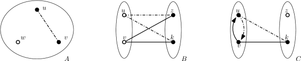
Figure 1: Nodes in the same community are circled, and they are labeled either with white or with black. In graph $A$ we see that the event “$u$ gets color black” implies the existence of edge $(u,v)$, then $\mathbf{P}\left(\mbox{$u$ gets color black}\,\middle|\,\mbox{$v$ gets color black}\right)\neq\mathbf{P}\left(\mbox{$u$ gets color black}\right)$. In graph $B$ we clearly see that, since $v$ and $u$ does not share any edge toward the other community, these edges do not yield stochastic dependence. In graph $C$, we see that if the edges inside each community are directed, then the presence of bold-drawn edges do not affect the presence of dashed-drawn edges.

Remark. Observe that, departing from the previous phases, we now need to analyze the label-spreading of the above rule over nodes having previously-assigned labels. This rises the following stochastic dependence. The analysis of the previous phases relies on the independence of the random variables (r.v.s) that correspond to the events “$u$ gets label $z_{i}$” for every label $i$ and every $u$ in a fixed community $\mathcal{V}$: let’s enumerate such r.v.s as $\{X_{u}\,|\,u\in\mathcal{V}\}$. Given a node $u$ and a set of nodes $S$, $E(u,S)$ denotes the set of edges from $u$ to any node in $S$. The r.v. $X_{u}$ depends on the edges incident to $u$; so, for any pair $u,v$ we can write $X_{u}=X_{u}((u,v),E(u,\mathcal{V}\setminus\{v\}),E(u,V\setminus\mathcal{V}))$ and $X_{v}=X_{v}((v,u),E(v,\mathcal{V}\setminus\{u\}),E(v,V\setminus\mathcal{V}))$. Since in our undirected-graph model $(u,v)$ equals $(v,u)$ then $X_{u}$ and $X_{v}$ share the argument $(u,v)$: this clearly yield stochastic dependence between them (see Fig. 1). However, if the graph of $\mathcal{V}$ is made directed, they become functions of disjoint sets of edges, therefore $X_{1},...,X_{|\mathcal{V}|}$ become mutually independent. In order to make our graph directed, the nodes run a simple procedure link-proc  at the very beginning of every step. This procedure simulates a virtual $\mbox{dyn-}\mathcal{G}(n,p,q)$ where the edges inside each community $\mathcal{V}$ are generated according to a directed $G_{n/2,\tilde{p}}$ model, where $\tilde{p}=1-\sqrt{1-p}$. Moreover, the procedure makes the resulting probability of the edges between communities still bounded by $O(q)$: it thus preserves the polynomial gap between $p$ and $q$. The proofs of these facts are given in App. D.4.

Procedure link-proc:

1. Each node $u$, for each neighbor $v$ generates a pair $(M^{u}(v),C^{u}(v))$ where $M^{u}(v)$ is a an integer randomly sampled from $[n^{3}]$, and $C^{u}(v)$ is $1$ or $-1$, each with probability $\frac{\sqrt{1-p}-1+p}{p}$ and $0$ with probability $\frac{(1-\sqrt{1-p})^{2}}{p}$.

2. $u$ sends this pair to $v$ (so it receives from $v$ the pair $(M^{v}(u),C^{v}(u))$).

3. If $M^{u}(v)>M^{v}(u)$ then $u$ defines $D^{u}(v)=C^{u}(v)$, otherwise if $M^{u}(v)<M^{v}(u)$ then $D^{u}(v)=-C^{v}(u)$.

4. Finally, $v$ is a (directed) neighbor of $u$ iff $D^{u}(v)\not=-1$.

Observe that we can neglect the event $M^{u}(v)=M^{v}(u)$ since its probability is $\frac{1}{n^{3}}$: if this happens we assume that both nodes virtually remove each other from their own neighborhood. In the sequel, we implicitly assume that nodes apply Procedure link-proc  and the Protocol-Window of Phase 4 is repeated 3 times for a specific setting of the constant $c_{4}$ that will be determined in (the proof of) Theorem 4. Thanks to Theorem 3, we can assume that the Markovian Process w.h.p. terminates Phase 3 reaching a state that satisfies Eq. 4. The proof of the next theorem is given in App. D.5.

Theorem 4

Let $\alpha$ be any constant such that $0<\alpha<1$. Then, constants $c_{4}$ and $a_{1}<1$ can be fixed so that, at time step $\tau_{4}=\tau_{3}+3T_{4}$, the Markovian Process w.h.p reaches a state such that, for $i=1,2$,

$$k_{i}^{\tau_{4}}\ \geqslant\ \alpha n\ ,\mbox{ and }h_{i}^{\tau_{4}}\ \leqslant\ n^{a_{1}}\ \mbox{\rm{polylog\,}}n.$$ (5)

Phase 5: Majority Rule. Theorem 4 states that, at the end of Phase 4, the Markovian Process w.h.p. reaches a state where a (large) constant fraction of the nodes (say, $3/4$) in both communities is well-labeled while only $O(n^{a_{1}}\mbox{\rm{polylog\,}}n)$ nodes are bad-labeled. We now show that a further final phase, where nodes apply a simple majority rule, yields the good labeling, w.h.p.. Remind that every node also applies Procedure link-proc shown in the previous phase. Every node $v\in V$ applies the following labeling rule:

• For every $t\in[1,T_{5}=c_{5}\log n]$, every node $v$ observes the labels of its neighbors at time $t$ and, for every label $z_{i}$ ($i=1,2$), $v$ computes the number $f^{t}_{i}$ of its neighbors labeled with $z_{i}$.

• Then, node $v$ gets label $z_{1}$ if $\sum_{t\in[1,\ldots,\tau_{5}]}f^{t}_{1}>\sum_{t\in[1,\ldots,\tau_{5}]}f^{t}_{2}$, otherwise $v$ gets label $z_{2}$ (break ties arbitrarily).

Let us assume the Markovian Process starts Phase 5 from a state satisfying Eq. 5 (say with constant $\alpha=3/4$). The proof of the next theorem is given in App. D.6.

Theorem 5

A constant $c_{5}>0$ can be fixed so that, at time $\tau_{5}=\tau_{4}+c_{5}\log n$, every node of each community is well-labeled, w.h.p.

Overall Completion Time of the Protocol and its Optimality

When $p$ and $q$ satisfy Cond. (1), we have shown that every phase has length $O(\log n)$: the Protocol has thus an overall completion time $O(\log n)$. In Appendix A, we will show that for $p=o(1/n)$ the length of each phase must be stretched to $\Theta\left(\frac{\log n}{pn}\right)$. It is easy to verify that, if $p=O(1/n)$, starting from the initial random snapshot, there is a non-negligible probability that some node will be isolated for $\tau(n)$ time steps where $\tau(n)$ is any increasing function such that $\tau=o\left(\frac{\log n}{pn}\right)$: this implies that, in the above range, our protocol has optimal completion time.

3 The General Setting

Removing the Presence of the Two Source Nodes. So far we have assumed that, in the initial state of the labeling process, there are exactly two source nodes, one in each community, which are labeled with different labels. This assumption can be removed by introducing a preliminary phase in which a randomized source election is performed and by some further changes that are described below.

In the first step, every node, by an independent random choice, becomes a source with probability $\frac{d\log n}{n}$ for a suitable constant $d>0$. This clearly guarantees that, in every community, there are w.h.p. $\Theta(\log n)$ sources. Then, every source $s_{i}$ randomly chooses a label $z_{i}\in[n^{2}]$. This implies that the minimal label $z_{1}$ in the first community and the minimal label $z_{2}$ in the second community are different w.h.p.. Let $a$ and $b$ be the number of sources chosen in $V_{1}$ and $V_{2}$, respectively, and define $\ell=a+b$. We summarize the above arguments in the following

Fact 1

Two positive constants $\eta_{1}<\eta_{2}$ exist such that at the end of the first step w.h.p. it holds that $\eta_{1}\log n\leqslant a,b\leqslant\eta_{2}\log n\ \mbox{ and }z_{1}\neq z_{2}$.

The generic state of the modified Markovian Process is represented by the following set of r.v.s:

$$(\ell_{1},\ell_{2};k^{1}_{1},\ldots,k^{1}_{a},h^{1}_{1},\ldots,h^{1}_{b},k^{2}_{1},\ldots,k^{2}_{b},h^{2}_{1},\ldots,h^{2}_{a})$$

where $k^{i}_{j}$ equals the number of nodes in $V_{i}$ labeled by the same (good) label as the $j$th source of $V_{i}$ while $h^{i}_{j}$ equals the number of nodes in $V_{i}$ labeled by the same (bad) label as the $j$th source of $V_{r}$ with $r\neq i$. At every time step $t$, for any $v\in[n]$ we define the r.v. $N_{j}^{v}(t)$ as the the number of $v$-neighbors labeled with label $z_{j}$ at time $t$.

The first three phases of the Protocol are identical to the 2-source case since the impact of the presence of an $O(\log n)$ labels in each of the two communities remains negligible till the overall number of labeled nodes in each community is $O(n/\log^{4}n)$. By applying the same analysis of the 2-source case, at the end of Phase 3, we can thus show that the Markovian Process w.h.p. reaches a state having similar properties to those stated in Theorem 3. We remind that $p$ and $q$ belong to the ranges in Cond. (1).

Theorem 6

We can choose a suitable $\tau_{3}=\tau_{2}+(c_{3}+o(1))\log n$ so that, at the end of Phase 3, the Markovian Process w.h.p. reaches a state in which for $\ell=1,2$ it holds

$$\forall j\in[a]\ \ \frac{n}{\log^{4}n}\ \leqslant\ k^{\ell}_{j}\ \leqslant\ \frac{n}{\log^{4-\eta}n}\ ;\ \forall i\in[b]\ \ h^{\ell}_{i}\ =\ \sqrt{n}\ \mbox{\rm{polylog\,}}n$$

where $\eta$ is a constant that can be made arbitrarily small.

We need to stop at a “saturation size” $O(n/\log^{4-\eta}n)$ for every good label, since we want to guarantee (w.h.p.) that the minimal label infects at least $n/\mbox{\rm{polylog\,}}n$ nodes. Then, as in the 2-source case, the protocol starts a controlled saturation phase (i.e. Phase 4) that consists of (at most) 4 consecutive time-windows in which every node applies the same following minimal-label rule:

For $t=1$ to $T_{4}=c_{4}\log n$ time steps, $v$ observes the labels of its neighbors and gets the minimal label $\hat{z}$ among all the observed labels.

Thanks to the above rule, the size of the nodes labeled by the minimal good-label increases by a logarithmic factor at the end of each of the four windows. This fact can be proved by using the same arguments of the proof of Theorem 4.

It thus follows that, at the end of Phase 4, the number of nodes labeled with the good minimal label is at least a constant (say $3/4$) fraction of all the nodes of the community. Then, as in the 2-source case, every node can apply the majority rule in order to get the right label w.h.p.

The Case $p$-unknown. Our protocol relies on the fact that nodes know the parameter $p=\frac{d}{n}$: the length of the protocol’s phases are functions of $p$. So an interesting issue is to consider the scenario where nodes do not know the parameter $p$ (i.e. the expected degree). Thanks to edge independence, the dynamic random-graph process can be seen by every node as an independent sequence of random samples. Indeed, at every time step $t$, every node can store the number $|N^{v}(t)|$ of its neighbors and it knows that this number has been selected by $n-1$ independent experiments according to the same Bernoulli distribution with success probability $p=\frac{d}{n}$. The goal is thus to use such samples in order to get a good approximation of $p$. If $p\geqslant\frac{1}{n}$, by using a standard statistical argument, every node w.h.p. will get the value of $p$ up to some negligible factor in $O(\log n)$ time. Let’s see this task more formally.

For $c\log n$ time steps (where $c$ is a constant that will be fixed later), every node stores the values $|N^{v}(1)|,|N^{v}(2)|,...,|N^{v}(c\log n)|$; then it computes $S=|N^{v}(1)|+\ldots+|N^{v}(c\log n)|$. Since $S$ is the sum of $c\log n\cdot(n-1)$ Bernoulli r.v.s of parameter $\frac{d}{n}$, we get a binomial distribution with mean $\mathbf{E}\left[S\right]=dc\log n\left(1-\frac{1}{n}\right)$ Then, every node uses the estimator $D(S)=\frac{S}{c\log n\ \left(1-\frac{1}{n}\right)}$ to guess $d$. We can use the Chernoff bound in order to determine a confidence interval for $D(S)$, as follows

$$\mathbf{P}\left(d\notin\ [D(S)-\delta,D(S)+\delta]\right)=\mathbf{P}\left(S\notin[\mathbf{E}\left[S\right]-\delta c\log n\ \frac{n-1}{n},\mathbf{E}\left[S\right]+\delta c\log n\ \frac{n-1}{n}\right)=$$

$$\mathbf{P}\left(S<\mathbf{E}\left[S\right]\left(1-\frac{\delta}{d}\right)\right)+\mathbf{P}\left(S>\mathbf{E}\left[S\right]\left(1+\frac{\delta}{d}\right)\right)<e^{-\frac{\delta^{2}}{2d^{2}}\mathbf{E}\left[S\right]}+e^{-\frac{\delta^{2}}{3d^{2}}\mathbf{E}\left[S\right]}<4\left(\frac{1}{n^{c}}\right)^{\frac{\delta^{2}}{3d}}$$

It thus follows that, for any $d\geqslant 1$, we can choose $\delta=\sqrt{d}$ and $c$ sufficiently large in order to get a good confidence interval for all nodes of the network. This obtained approximation suffices to perform an analysis of the protocol which is equivalent to that of the case $p$-known.

More Communities. The presence of a constant number $r=\Theta(1)$ of unknown equally-sized communities can be managed with a similar method to that described above for removing the presence of leaders. Indeed, the major issue to cope with is the presence of a constant number of different label spreadings in each community and the protocol must select the right one in every community. However, if $r$ is a constant and the number of nodes in each community is some constant fraction of $n$, then the impact of the presence of $O(\log n)$ labels in each of the $r$ communities remains negligible till the overall number of labeled nodes in each community is $O(n/\log^{4}n)$. As in the previous paragraph, by first applying the minimal-label rule and then the majority one, the modified protocol returns a good-labeling w.h.p.

Due to lack of space, the protocol analysis in the Edge-MEG model is given in Appendix.

4 Conclusions

This paper introduces a framework that allows an analytical study of the distributed community-detection problem in dynamic graphs. Then, it shows an efficient algorithmic solution in two classes of such graphs that model some features of opportunistic networks such as ICMNs. We believe that the problem deserves to be studied in other classes of dynamic graphs that may capture further relevant features of social opportunistic networks such as geometric constraints.

Acknowledgements. We thank Stefano Leucci for its help in getting an efficient protocol simulation over large random graphs.

Appendix A More General Settings (Part II)

In this section, we show the further relevant generalizations that can be efficiently solved by simple adaptations of our protocol and/or its analysis.

Edge Markovian Evolving Graphs. Let us consider an Edge-MEG $\mbox{dyn-}\mathcal{G}(n,p_{\uparrow},p_{\downarrow},q_{\uparrow},q_{\downarrow},E_{0})$ defined in the introduction and assume that $q_{\uparrow}\leqslant p_{\uparrow}/n$. If $0<p_{\uparrow},p_{\downarrow},q_{\uparrow},q_{\downarrow}<1$, it is easy to see [12] that the (unique) stationary distribution of the two corresponding 2-state edge-Markov chains (inside and outside the communities, respectively) are

$$\mathbf{\pi^{in}}\ =\ \left(\frac{p_{\downarrow}}{p_{\uparrow}+p_{\downarrow}},\frac{p_{\uparrow}}{p_{\uparrow}+p_{\downarrow}}\right)\ \mbox{ and }\ \mathbf{\pi^{out}}\ =\ \left(\frac{q_{\downarrow}}{q_{\uparrow}+q_{\downarrow}},\frac{q_{\uparrow}}{q_{\uparrow}+q_{\downarrow}}\right)$$

It thus follows that the dynamic graph, starting from any $E_{0}$, converges to the (2-communities) Erdös-Rényi random graph with edge-probability functions

$$\tilde{p}\ =\ \frac{p_{\uparrow}}{p_{\uparrow}+p_{\downarrow}}\ \mbox{ (inside communities) }\ \mbox{ and }\tilde{q}\ =\ \frac{q_{\uparrow}}{q_{\uparrow}+q_{\downarrow}}\ \mbox{ (outside communities)}$$

The mixing time $M^{in}$ and $M^{out}$ of the two edge Markov chain are bounded by [12] $M^{in}\ =\ O\left(\frac{1}{p_{\uparrow}+p_{\downarrow}}\right)$ , $M^{out}\ =\ O\left(\frac{1}{q_{\uparrow}+q_{\downarrow}}\right)$. Let us observe that there is a Markovian dependence between graphs of consecutive time steps. If we observe any event at time $t$ related to $E_{t}$ (such as the number of well-labeled nodes) then $E_{t+1}$ is not anymore random with the stationary distribution.

It thus follows that we need to change the way the protocol works over the dynamic random graph. Let $M=\max\{M^{in},M^{out},\log n\}$; then by definition of mixing time, starting from any edge subset $E_{t}$ at time $t$, at time $t+\Delta$ with some $\Delta=\Theta(M)$, if $u,v\in V_{1}$ or $u,v\in V_{2}$ then edge $(u,v)$ exists with probability $\tilde{p}\pm\frac{1}{n^{2}}$, otherwise it exists with probability $\tilde{q}\pm\frac{1}{n^{2}}$. In other words, whathever the state of the labeling process is at time $t$, after a time window proportional to the mixing time, the dynamic graph is random with a distribution which is very close to the stationary one. We can thus modify our protocol for the dynamic Erdös–Rényi graph model $\mbox{dyn-}\mathcal{G}(n,p,q)$ in order to “wait for mixing”. Between any two consecutive steps of the original protocol there is a quiescent time-window of length $\Theta(M)$ where every node simply does nothing. Then, the analysis of the protocol over $\mbox{dyn-}\mathcal{G}(n,p_{\uparrow},p_{\downarrow},q_{\uparrow},q_{\downarrow},E_{0})$ is similar to that in Section LABEL:sec::2-source working for the dynamic Erdös–Rényi graph $\mbox{dyn-}\mathcal{G}(n,\tilde{p},\tilde{q})$. We can thus state that, under the condition $q_{\uparrow}\leqslant O(p_{\uparrow}/n^{b})$ for some constant $b>0$, this version of our protocol w.h.p. performs a good-labeling in time $O\left(M\cdot\max\left\{\log n,\frac{\log n}{pn}\right\}\right)$. We finally observe that, for the “realistic” case $p_{\downarrow},q_{\downarrow}=\Theta(1)$ (see the discussion in the Introduction), the mixing-time bound $M$ turns out to be $O(\log n)$: we thus get only a logarithmic slowdown-factor w.r.t. the good-labeling in the dynamic Erdös–Rényi graph $\mbox{dyn-}\mathcal{G}(n,\tilde{p},\tilde{q})$.

Sparse Graphs. When $p=o\left(\frac{1}{n}\right)$ and $\frac{q}{p}=O\left(\frac{1}{n^{b}}\right)$ (for some constant $b>0$), the snapshots of the dynamic graph are very sparse. So, every node must wait at least $\Theta\left(\frac{1}{pn}\right)$ time step (in average) in order to meet some other node. This implies that the labeling protocol will be slower. We can reduce this case to the case $p=1/n$ by considering the time-union random graph obtained from $\mbox{dyn-}\mathcal{G}(n,p,q)$ according to the following

Definition 7

Let $\Delta$ be any positive integer and consider any sequence of graphs $G(V,E_{1}),\ldots,G(V,E_{\Delta})$. Then, we define the $\Delta$-OR-graph

$$G_{\vee}^{\Delta}=\left(V,E^{\Delta}\right)\ \text{ where }\ E^{\Delta}\ =\ \{e\in\binom{n}{2}\ |\ \exists t^{\star}\in(1,\Delta]\ :\ e\in E_{t^{\star}}\}$$

It is easy to prove the following

Lemma 8

Let $p<\frac{1}{n}$, then the $\frac{1}{pn}$-OR-graph of any finite sequence of graphs selected according to the $\mbox{dyn-}\mathcal{G}(n,p,q)$ model is a $\mbox{dyn-}\mathcal{G}(n,\tilde{p},\tilde{q})$ with $\tilde{p}=\Theta\left(\frac{1}{n}\right)$ and $\tilde{q}=O\left(\frac{p}{n^{b}}\right)$.

The modified protocol just works as it would work over $\mbox{dyn-}\mathcal{G}(n,\tilde{p},\tilde{q})$ with $\tilde{p}=\Theta\left(\frac{1}{n}\right)$ and $\tilde{q}=O\left(\frac{p}{n^{b}}\right)$: in every phase, every node applies the phase’s labeling rule (only) every $\Delta=\frac{1}{pn}$ time steps on the $\frac{1}{pn}$-OR-graph. The modified protocol thus requires $\Theta\left(\Delta\log n\right)=\Theta\left(\frac{\log n}{pn}\right)$ time.

Dense Graphs. When $p$ becomes larger than $\log n/n$ and $q=\left(\frac{p}{n^{b}}\right)$, the labeling problem becomes an easier task since standard probability arguments easily show that the (good) labeling process is faster and the related r.v.s (i.e. number of new labeled nodes at every time step) have much smaller variance. This implies that the protocol can be simplified: for instance, the source-labeling phase (i.e. Phase 1) can be skipped while the length of other phases can be reduced significantly as a function of $p$. However, we again emphasize that dense dynamic random random graphs are not a good model for the scenario we are inspired from: ICMNs are opportunistis networks having sparse and disconnected topology.

Appendix B Experimental Results

We run our protocol over sequences of independent random graphs according to the $\mbox{dyn-}\mathcal{G}(n,p,q)$ model. The protocol has been suitably simplified and tuned in order to optimize the real performance. In particular, the implemented procotol consists of 5 Phases: Phase 1 (Source-Coloring), Phase 2-3 (Fast-Coloring I-II), Phase 4 (Min-Coloring), and Phase 5 (Majority-Rule). The rules of each phase is the same of the corresponding phase analyzed in Section LABEL:sec::2-source. Moreover, the length of every phase is fixed to $c\log n$. As shown in the next tables, parameter $c$ is always very small and it depends on the parameter $q$. The parameter $c$ has been heuristically chosen as the minimal one yielding the good labeling in more than $98\%$ of the trials. We consider instances of increasing size $n$ and for each size, we tested 100 random graphs. In the first experiment class (see Table 1), we consider homogeneous sparse graphs with the following setting: $p=\frac{5}{n}$ and 3 values of $q$ ranging from $1/n^{2}$ to $1/n^{3/2}$.

Table 1: Tab. 1. Experimental results for the homogeneous case. For every value of $n$, the rows indicates the percentage of good-labeling for three choices of $q$ and the “minimal” setting for $c$ (the total number of Protocol’ steps is inside brackets).

n	$q=n^{-\frac{3}{2}},c=0.9$	$q=n^{-\frac{5}{3}},c=0.6$	$q=n^{-2},c=0.5$
20000	99 (66)	100 (46)	100 (36)
40000	99 (71)	100 (46)	100 (41)
80000	100 (76)	100 (51)	100 (41)
160000	100 (81)	100 (51)	100 (46)
320000	100 (86)	100 (56)	99 (46)
640000	100 (91)	100 (61)	100 (51)
1280000	100 (91)	100 (61)	100 (51)
2560000	100 (96)	100 (66)	100 (56)

The second class of experiments concerns non-homogeneous random graphs. For each pair of nodes $e=(u,v)$ in the same community, the probability $p_{e}$ is randomly fixed in a range $[d_{1}/n,d_{2}/n]$ before starting the graph-sequence generation. Then, a every time step $t\geqslant 0$, the graph-snapshot $G(V,E_{t})$ is generated by selecting every edge $e=(u,v)$ according to its birth-probability $p_{e}$ (the edges between the two communities are generated with parameter $q$). In Table 2, the experimental results are shown for the case $d_{1}=1$ and $d_{2}=9$ in order to generate sparse topologies inside the communities, while in Table 3, the results concern the more dense case where $d_{1}=0$ and $d_{2}=\log n$. The protocol’s implementation is the same of the homogeneous case above.

Table 2: Tab. 2. Experimental results for the non-homogeneous sparse case with $d_{1}=1$ and $d_{2}=9$.

$n$	$q=1/n^{3/2},c=1$	$q=1/n^{5/3},c=0.4$	$q=1/n^{2},c=0.4$
20000	100 (46)	100 (46)	100 (36)
40000	98 (71)	99 (46)	100 (41)
80000	100 (76)	100 (51)	100 (41)
160000	100 (81)	100 (51)	100 (46)
320000	100 (86)	100 (56)	100 (46)
640000	100 (91)	100 (61)	100 (51)
1280000	100 (91)	100 (61)	100 (51)

Table 3: Tab. 3. Experimental results for the non-homogeneous case with $d_{1}=0$ and $d_{2}=\log n$.

$n$	$q=n^{-\frac{3}{2}},c=1$	$q=n^{-\frac{5}{3}},c=0.4$	$q=n^{-2},c=0.4$
20000	99 (76)	100 (31)	100 (31)
40000	99 (81)	100 (31)	100 (31)
80000	98 (86)	100 (31)	100 (31)
160000	100 (91)	100 (36)	100 (36)
320000	100 (96)	100 (36)	100 (36)
640000	100 (101)	100 (41)	100 (41)
1280000	100 (106)	100 (41)	100 (41)

The experiments globally show that the tuning of parameter $c$ mainly depends on the value of $q$ even though it can be fixed to small values in all studied cases. Moreover, the presence of non-homogeneous edge-probability function seems to slightly “help” the efficiency of the protocol. Intuitively speaking, we believe this is due to the presence of fully-random irregularities in the graph topology that helps the protocol to break the symmetry of the initial configuration.

Appendix C Useful Tools

Lemma 9

If $x=o(1)$ and $xy=o(1)$ then

$$\left(1-x\right)^{y}\geqslant 1-xy\left(1+2x\right)$$

$$\left(1-x\right)^{y}\leqslant 1-xy\left(1-xy\right)$$

We will often use the Chernoff’s bounds

Lemma 10 (Chernoff’s Bound.)

Let be $X=\sum_{i=1}^{n}X_{i}$ where $X_{1},\dots,X_{n}$ are independent Bernoulli r.v.s and let be $0<\delta<1$. If $0<\mu_{1}\leq\mathbf{E}[X]$ and $\mu_{2}\geq\mathbf{E}\left[X\right]$, then it holds that

$$\mathbf{P}\{X\leq(1-\delta)\mu_{1}\}\leq e^{-\frac{\delta^{2}}{2}\mu_{1}}.$$ (6)

$$\mathbf{P}\left(X\geq(1+\delta)\mu_{2}\right)\leq e^{-\frac{\delta^{2}}{3}\mu_{1}}.$$ (7)

Lemma 11

Let $\varphi$ be any poly-logarithm and $E_{0}$, $E_{1}$, …, $E_{\varphi}$ be events that hold w.h.p., then $E_{0}\cap E_{1}\cap...\cap E_{\varphi}$ holds w.h.p.

Appendix D Proofs of the Protocol’s Analysis

In the sequel, we always analyze the Markovian process in Community $V_{1}$ since the analysis in the second community is the same.

D.1 The Source Labeling: Proof of Theorem 1

We define the following r.v.s counting the labeled nodes at the end of Phase 1.

• The variable $X_{1}^{v}=1$ iff $v$ gets label $z_{1}$, and the variable $X_{1}=1+\sum\limits_{v\neq s_{1}}X_{1}^{v}$ describes the total number of the $z_{1}$-labeled nodes in $V_{1}$.

• The variable $Y_{1}^{v}=1$ iff $v$ gets label $z_{2}$, and the variable $Y_{1}=\sum\limits_{v\neq s_{1}}Y_{1}^{v}$ describes the total number of the $z_{2}$-labeled nodes in $V_{1}$.

In order to prove the theorem we need the following lemmas.

Lemma 12

Let $\tau_{1}$ be such that $p\tau_{1}\geqslant\frac{\log n}{n}$ and $\tau_{1}=o\left(\frac{1}{p}\right)$. Then, starting from the initial state $\left(k_{1}^{(0)}=1,k_{2}^{(0)}=1,h_{1}^{(0)}=0,h_{2}^{(0)}=0;E_{0}\right)$, at time step $\tau_{1}$ w.h.p. it holds that

$$\frac{1}{16}np\tau_{1}\ \leqslant X_{1},X_{2}\ \leqslant\ 4np\tau_{1}$$

Proof. We first bound from below the number of $z_{1}$-labeled nodes at the end of the Phase 1. Notice that $\mathbf{P}\left(X_{1}^{v}=1\right)=\left(1-q\right)^{\tau_{1}}\left(1-\left(1-p\right)^{\tau_{1}}\right)$ and we can apply Lemma 9 to each factor on the right side, getting:

$$\mathbf{P}\left(X_{1}^{v}=1\right)=\left(1-q\right)^{\tau_{1}}\left(1-\left(1-p\right)^{\tau_{1}}\right)\geqslant p\tau_{1}\left[\left(1-q\tau_{1}\left(1+{2q}\right)\right)\left(1-p\tau_{1}\right)\right]\geqslant\frac{p\tau_{1}}{2}$$

where in the last inequality we used $\lim_{n\rightarrow\infty}\left[\left(1-q\tau_{1}\left(1+{2q}\right)\right)\left(1-p\tau_{1}\right)\right]=1$.

The above inequality easily implies that

$$\mathbf{E}\left[X_{1}\right]=1+(|V_{1}|-1)\cdot\mathbf{P}\left(X_{1}^{v}=1\right)\ \geqslant\ 1+\left(\frac{n}{2}-1\right)\frac{p\tau_{1}}{2}\ >\ \frac{n}{2}\left(1-\frac{2}{n}\right)\frac{p\tau_{1}}{2},$$

that is

$$\mathbf{E}\left[X_{1}\right]>\frac{np\tau_{1}}{8}$$

Since, by fixing any initial state $\left(k_{1}^{(0)},k_{2}^{(0)},h_{1}^{(0)},h_{2}^{(0)};E_{0}\right)$, the r.v.s $X_{1}^{v}$ are independent, we can apply the Chernoff Bound (6) with $\delta=\frac{1}{2}$. Then,

$$\mathbf{P}\left(X_{1}\leqslant\frac{np\tau_{1}}{16}\right)\leqslant e^{-\frac{1}{64}np\tau_{1}}$$

By hypothesis, we have that $np\tau_{1}\geqslant\log n$, so, w.h.p. it holds that

$$X_{1}\geqslant\frac{np\tau_{1}}{16}$$

A similar analysis, based on Lemma 9 and Chernoff bound (7), yields the stated upper bound on the number of $z_{1}$-labeled nodes at the end of the Phase 1, that is, w.h.p. it holds that

$$X_{1}\leqslant 4np\tau_{1}$$

Lemma 13

Let $\tau_{1}\geqslant 1$ be such that $q\tau_{1}=O\left(\frac{1}{n^{1+\epsilon}}\right)$ for any $\epsilon>0$. Then, starting from the initial state $\left(k_{1}^{(0)}=1,k_{2}^{(0)}=1,h_{1}^{(0)}=0,h_{2}^{(0)}=0;E_{0}\right)$, at time step $\tau_{1}$ it holds w.h.p. that $Y_{1}=0$.

Proof. A sufficient condition for having $Y_{1}=0$ is that no edge between any node in $V_{1}$ and $s_{2}$ occurs at any time step of Phase 1. Hence, by Lemma 9,

$$\mathbf{P}\left(Y_{1}=0\right)\geqslant\left(1-q\right)^{|V_{1}|\tau_{1}}=\left(1-q\right)^{\frac{n\tau_{1}}{2}}\geqslant 1-2q|V_{1}|\tau_{1}$$

Since $q\tau_{1}=O(\frac{1}{n^{1+b}})$, the lemma is proved.

Lemmas 12 and 13 easily imply the theorem.

D.2 Fast Labeling I: Proof of Theorem 2

We remind that $q=O(p/n^{b})$ and consider any positive constant $a$ such that $a<b$. We consider the Markovian Process when, at the generic step $t$ of this phase, it is in any state satisfying the following condition:

$$k_{1}^{(t)},k_{2}^{(t)}\in\left[\frac{d_{1}}{16}pn\log n,d_{1}pn^{1+a}\log n\right]\text{ and }h_{1}^{(t)},h_{2}^{(t)}=0$$ (8)

For each time step $t$, $\tau_{1}<t\leqslant\tau_{1}+\tau_{2}$, we define the following binary r.v.s

• $X_{1}^{v}(t)=1$ iff $v\in V_{1}$ gets label $z_{1}$ at time $t+1$, and $X_{1}(t)=\sum\limits_{v\in V_{1}}X_{1}^{v}(t)$.

• $Y_{1}^{v}(t)=1$ iff $v\in V_{1}$ gets label $z_{2}$ at time $t+1$, and $Y_{1}(t)=\sum\limits_{v\in V_{1}}Y_{1}^{v}(t)$

The first lemma provides tight upper and lower bounds on the number of new labeled nodes after one step of the protocol. The choice of $\tau_{2}$ will be given later in Theorem 2.

Lemma 14

For $i=1,2$, it holds w.h.p. that

$$\left(1-\sqrt{\frac{\log n}{k_{i}^{(t)}}}\right)\left(1-\frac{\mbox{\rm{polylog\,}}n}{n^{1-a}}\right)\,\frac{np}{2}k_{i}^{(t)}\leqslant X_{i}(t)\ \leqslant\left(1+\sqrt{\frac{\log n}{k_{i}^{(t)}}}\right)\left(1+\frac{\mbox{\rm{polylog\,}}n}{n^{1-a}}\right)\,\frac{np}{2}k_{i}^{(t)}$$

$$Y_{i}(t)\ =\ 0.$$

Proof. Observe that $\mathbf{P}\left(Y_{1}(t)=0\right)$ is lower bounded by the probability that in $E_{t}$ there is no edge between any node in $V_{1}$ and any node in $V_{2}$ which is already labeled $z_{2}$. By the hypothesis (8) and the conditions on $p$ and $q$, we can thus apply Lemma 9 and get

$$\mathbf{P}\left(Y_{1}=0\right) \geqslant\left(1-q\right)^{|V_{1}|k_{2}^{(t)}}\geqslant 1-2q|V_{1}|k_{2}^{(t)}\geqslant 1-\frac{\mbox{\rm{polylog\,}}n}{n^{1-a}}$$

proving that w.h.p. $Y_{1}(t)=0$. Again, thanks to Condition (8) and the conditions on $p$ and $q$ (Eq. 1), we can apply Lemma 9 to bound $\mathbf{P}\left(X_{1}^{v}=1\right)=\left(1-\left(1-p\right)^{k_{1}^{(t)}}\right)\left(1-q\right)^{k_{2}^{(t)}}$. We get

$$\mathbf{P}\left(X_{1}^{v}=1\right) \geqslant k_{1}^{(t)}p\left(1-k_{1}^{(t)}p\right)\left(1-2k_{2}^{(t)}q\right)\geqslant k_{1}^{(t)}p\left(1-\frac{\mbox{\rm{polylog\,}}n}{n^{1-a}}\right)$$

$$\mathbf{P}\left(X_{1}^{v}=1\right) \leqslant k_{1}^{(t)}p\left(1+2p\right)\leqslant k_{1}^{(t)}p\left(1+\frac{\mbox{\rm{polylog\,}}n}{n^{1-a}}\right)$$

We can thus bound the expected number of new well-labeled nodes $\mathbf{E}\left[X_{1}\right]=\left(|V_{1}|-k_{1}^{(t)}\right)\mathbf{P}\left(X_{1}^{v}=1\right)$:

$$\frac{np}{2}k_{1}^{(t)}\left(1-\frac{\mbox{\rm{polylog\,}}n}{n^{1-a}}\right)\leqslant\mathbf{E}\left[X_{1}\right]\leqslant\frac{np}{2}k_{1}^{(t)}\left(1+\frac{\mbox{\rm{polylog\,}}n}{n^{1-a}}\right)$$

By applying the Chernoff Bounds (6) and ((7)) with $\delta=\sqrt{\frac{\log n}{k_{1}}}$, we get

$$\mathbf{P}\left(X_{1}\leqslant\left(1-\sqrt{\frac{\log n}{k_{1}^{(t)}}}\right)\left(1-\frac{\mbox{\rm{polylog\,}}n}{n^{1-a}}\right)\,\frac{np}{2}k_{1}^{(t)}\right) =e^{-\frac{\log n}{2k_{1}^{(t)}}\frac{np}{2}k_{1}^{(t)}\left(1-\frac{\mbox{\rm{polylog\,}}n}{n^{1-a}}\right)}\leqslant\frac{1}{n^{\frac{1}{3}}}$$

$$\mathbf{P}\left(X_{1}\geqslant\left(1+\sqrt{\frac{\log n}{k_{1}^{(t)}}}\right)\left(1+\frac{\mbox{\rm{polylog\,}}n}{n^{1-a}}\right)\,\frac{np}{2}k_{1}^{(t)}\right) =e^{-\frac{\log n}{3k_{1}^{(t)}}\frac{np}{2}k_{1}^{(t)}\left(1-\frac{\mbox{\rm{polylog\,}}n}{n^{1-a}}\right)}\leqslant\frac{1}{n^{\frac{1}{3}}}$$

This implies that, w.h.p.,

$$\left(1-\sqrt{\frac{\log n}{k_{1}^{(t)}}}\right)\left(1-\frac{\mbox{\rm{polylog\,}}n}{n^{1-a}}\right)\,\frac{np}{2}k_{1}^{(t)}\leqslant X_{1}(t)\ \leqslant\left(1+\sqrt{\frac{\log n}{k_{1}^{(t)}}}\right)\left(1+\frac{\mbox{\rm{polylog\,}}n}{n^{1-a}}\right)\,\frac{np}{2}k_{1}^{(t)}$$

In what follows, we will make use of the following function

$$F(n,k)=2\max\left\{\sqrt{\frac{\log n}{k}},\frac{\mbox{\rm{polylog\,}}n}{n^{1-a}}\right\}$$

Let us observe that $k_{i}^{(t+1)}=k_{i}^{(t)}+X_{i}(t)$. So, Lemma 14 implies the following recursive bounds

Lemma 15

For $i=1,2$, it holds w.h.p. that

$$\left(1+\frac{np}{2}\right)\left[1-F(n,k_{i}^{(t)})\right]k_{i}^{(t)} \leqslant{k_{i}^{(t+1)}}\ \leqslant\left(1+\frac{np}{2}\right)\left[1+F(n,k_{i}^{(t)})\right]k_{i}^{(t)}$$

and $$\ {h_{i}^{(t+1)}}\ =\ 0.$$

Proof of Theorem 2. We first analyze the good labeling. The idea is to derive the closed formula corresponding to the recurrence relation provided by Lemma 15 and to analyze it in two different spans of time: in the first span, we let $k_{1}$ increase enough so that, in the second span, we can apply a stronger concentration result. Recall that, thanks to Theorem 1, Phase 2 starts with the Markovian Process in a state satisfying Condition (2) that implies Condition (8). Moreover, we will fix the final time step $\tau_{2}$ so that Condition (8) has been holding for all time steps of Phase 2: this implies that we can apply Lemma 15 for all such steps.

Let $t^{*}\leqslant\tau_{1}$ be defined as

$$t^{\star}={\log^{-1}\left(\left(1+\dfrac{np}{2}\right)\left(1-F(n,k_{1}^{(\tau_{1})})\right)\right)}\log\left(\frac{\log^{3}n}{k_{1}^{(\tau_{1})}}\right)+\tau_{1}.$$

Since $t^{*}-\tau_{1}\in O(\log n)$, thanks to Lemma 11, we can unroll (backward) the recursive relation from time $t^{\star}$ to time $\tau_{1}$ and get

$$\left(1+\frac{np}{2}\right)^{t^{\star}-\tau_{1}}\left[1-F(n,k_{1}^{(\tau_{1})})\right]^{t^{\star}-\tau_{1}}k_{1}^{(\tau_{1})}\leqslant{k_{1}^{(t^{\star})}}\ \leqslant\left(1+\frac{np}{2}\right)^{t^{\star}-\tau_{1}}\left[1+F(n,k_{1}^{(\tau_{1})})\right]^{t^{\star}-\tau_{1}}k_{1}^{(\tau_{1})}$$ (9)

We observe that the value of $k_{1}^{\tau_{1}}\geqslant\frac{d_{1}}{16}pn\log n$ can reach any arbitrarily large constant by tuning the constant $d_{1}$ in Theorem 1; so, $F(n,k_{1}^{(\tau_{1})})$ can be made arbitrarily small. From this fact and Eq. 9, we have that $k_{1}^{(t^{\star})}\in\left[\log^{3}n,\log^{3+\mu}n\right]$, where $\mu$ can be made arbitrarily small by decreasing $F(n,k_{1}^{(\tau_{1})})$ (i.e. by increasing $d_{1}$ in Theorem 1). Notice that, at any time step $t\leqslant t^{*}$, Condition (8) is largely satisfied.

We now unroll the recursive relation from time $\tau_{2}$ to time $t^{\star}$ and get

$$\left(1+\frac{np}{2}\right)^{\tau_{2}-t^{\star}}\left[1-F(n,k_{1}^{(t^{\star})})\right]^{\tau_{2}-t^{\star}}k_{1}^{(t^{\star})}\leqslant{k_{1}^{(\tau_{2})}}\ \leqslant\left(1+\frac{np}{2}\right)^{\tau_{2}-t^{\star}}\left[1+F(n,k_{1}^{(t^{\star})})\right]^{\tau_{2}-t^{\star}}k_{1}^{(t^{\star})}.$$ (10)

We observe that, with a suitable choice of the positive constant $\phi\in(0,1)$, for

$$\tau_{2}=\log^{-1}\left(1+\frac{np}{2}\right)\log\left(\frac{n^{a}}{\phi\log^{3}n}\right)+t^{\star}$$

it holds that

$$\left[1-F(n,k_{1}^{(t^{\star})})\right]^{\tau_{2}-t^{\star}}\geqslant\phi\mbox{\hskip 28.45274pt and \hskip 28.45274pt}\left[1+F(n,k_{1}^{(t^{\star})})\right]^{\tau_{2}-t^{\star}}\leqslant\frac{1}{\phi}$$

By replacing $\tau_{2}$ into Eq. 10, with a suitable choice of $\eta\geq\mu$ (remind that $\mu$ can in turn be made arbitrarily small), we finally get $n^{a}\leqslant k_{1}^{(\tau_{2})}\leqslant n^{a}\log^{\eta}n$. Again, observe that, for all time steps $t\leqslant\tau_{2}$, Condition (8) is largely satisfied: this implies that at each of these steps we were able to apply Lemma 15.

As for the bad labeling, observe that Lemma 15 guarantees (w.h.p.) ${h}_{1}^{(t)},{h}_{2}^{(t)}=0$; then, from Lemma 11, it holds w.h.p that ${h}_{1}^{(\tau_{2})}=0$ and ${h}_{2}^{(\tau_{2})}=0$.

D.3 Fast Labeling II: Proof of Theorem 3

We consider the Markovian Process when, at the generic step $t$ of this phase, it is in any state satisfying the following condition

$$\mbox{ for }\ i=1,2\ :\ \ k_{i}^{(t)}\in\left[n^{a},\frac{{n}}{\log^{2}n}\right]\ \text{ and }h_{i}^{(t)}\ =O(n^{a_{2}}),\ \mbox{where $a_{1}<a_{2}<1$}$$ (11)

For each time step $t$, $\tau_{1}<t\leqslant\tau_{1}+\tau_{2}$, we again consider the following binary r.v.s

• $X_{1}^{v}(t)=1$ iff $v\in V_{1}$ gets label $z_{1}$ at time $t+1$, and $X_{1}(t)=\sum\limits_{v\in V_{1}}X_{1}^{v}(t)$.

• $Y_{1}^{v}(t)=1$ iff $v\in V_{1}$ gets label $z_{2}$ at time $t+1$, and $Y_{1}(t)=\sum\limits_{v\in V_{1}}Y_{1}^{v}(t)$

In all the next lemmas of this phase, it is assumed that, at the end of Phase 2, the Markovian Process is in a state satisfying Condition (11) (thanks to Theorem 2 this holds w.h.p.).

We start by providing, with the next lemma, tight upper and lower bounds on the number of the well-labeled nodes at a generic step of Phase 3.

Lemma 16

A constant $\zeta>0$ exists such that, for $i=1,2$, it holds w.h.p. that

$$\left(1+\frac{np}{2}\right)\left(1-\frac{\zeta}{\log n}\right)k_{i}^{(t)} \leqslant\ k_{i}^{(t+1)}\leqslant\ \left(1+\frac{np}{2}\right)\left(1+\frac{\zeta}{\log n}\right)k_{i}^{(t)}$$ (12)

Sketch of Proof. By neglecting the contribution of $h_{2}$, from the facts $pk_{1}^{(t)},qk_{2}^{(t)},ph_{1}^{(t)}=o(1)$ and Lemma 9, we have that

$$\mathbf{P}\left(X_{1}^{v}=1\right) \geqslant \left(1-\left(1-p\right)^{k_{1}^{(t)}}\right)\left(1-q\right)^{k_{2}^{(t)}}\left(1-p\right)^{h_{1}^{(t)}}$$

$$\geqslant pk_{1}^{(t)}\left(1-p{k_{1}^{(t)}}\right)\left(1-2q{k_{2}^{(t)}}\right)\left(1-2p{h_{1}^{(t)}}\right).$$

Observe that

$$\left(1-p{k_{1}^{(t)}}\right)\left(1-2q{k_{2}^{(t)}}\right)\left(1-2p{h_{1}^{(t)}}\right)\ \geqslant\ \left(1-\Theta\left(\frac{1}{\log^{2}n}\right)\right)$$

then

$$\mathbf{P}\left(X_{1}^{v}=1\right)\geqslant pk_{1}^{(t)}\left(1-\Theta\left(\frac{1}{\log^{2}n}\right)\right)$$ (13)

We now provide an upper bound on $\mathbf{P}\left(X_{1}^{v}=1\right)$. From the Union Bound and Lemma 9, we get

$$\mathbf{P}\left(X_{1}^{v}=1\right)\leqslant pk_{1}^{(t)}\left(1+2{p}\right)+qh_{2}^{(t)}\left(1+2{q}\right)\leqslant pk_{1}^{(t)}\left(1+\Theta\left(\frac{1}{n^{1-a_{2}}}\right)\right).$$ (14)

As usual, we exploit Eq.s 13 and 14 to bound the expectation

$$\mathbf{E}\left[X_{1}\right]=\left(|V_{1}|-(k_{1}^{(t)}+h_{1}^{(t)})\right)\cdot\mathbf{P}\left(X_{1}^{v}=1\right)$$

For some constant $\tilde{\zeta}>0$, w.h.p. it thus holds that

$$\frac{np}{2}k_{1}^{(t)}\left(1-\frac{\tilde{\zeta}}{\log n}\right)\leqslant\mathbf{E}\left[X_{1}\right]\leqslant\frac{np}{2}k_{1}^{(t)}\left(1+\frac{\tilde{\zeta}}{\log n}\right)$$

We can use the Chernoff Bounds (6 and 7 with $\delta={1}/{\log n}$), to get that, for some constant ${\zeta}>0$, w.h.p.

$$\frac{np}{2}k_{1}^{(t)}\left(1-\frac{\zeta}{\log n}\right)\leqslant X_{1}\leqslant\frac{np}{2}k_{1}^{(t)}\left(1+\frac{\zeta}{\log n}\right)$$ (15)

From the above inequality, it follows that

$$\left(1+\frac{np}{2}\right)\left(1-\frac{np}{2+np}\frac{\zeta}{\log n}\right)k_{1}^{(t)}\leqslant k_{1}^{(t+1)}\leqslant\left(1+\frac{np}{2}\right)\left(1+\frac{np}{2+np}\frac{\zeta}{\log n}\right)k_{1}^{(t)},$$

Since $\frac{np}{2+np}{\zeta}$ is bounded by a constant, for the sake of simplicity we can just re-define $\zeta$ as any fixed constant such that

$$\left(1+\frac{np}{2}\right)\left(1-\frac{\zeta}{\log n}\right)k_{1}^{t}\leqslant k_{1}^{t+1}\leqslant\left(1+\frac{np}{2}\right)\left(1+\frac{\zeta}{\log n}\right)k_{1}^{t}$$

Lemma 16 implies the following properties of the well-labeling for any state within Phase 3 (including the final one at time $\tau_{3}$).

Lemma 17

A constant $\zeta>0$ exists such that, for $i=1,2$, it holds w.h.p. that

$$\left(1+\frac{np}{2}\right)^{t+1-\tau_{2}}\left(1-\frac{\zeta}{\log n}\right)^{t+1-\tau_{2}}k_{1}^{(\tau_{2})}\leqslant k_{1}^{(t+1)}\leqslant\left(1+\frac{np}{2}\right)^{t+1-\tau_{2}}\left(1+\frac{\zeta}{\log n}\right)^{t+1-\tau_{2}}k_{1}^{(\tau_{2})}$$

Sketch of Proof. Since Lemma 16 holds as long as $k_{i}\leqslant\frac{n}{\log^{2}n}$, from Lemma 11 we get that the statement holds w.h.p. by applying the same unrollement argument shown in the previous phase.

We now exploit the above lemma to provide a bound on the number of bad-labeled nodes at the end of Phase 3.

Lemma 18

For any positive constant $\gamma$, a constant $a_{1}$, with $1-a<a_{1}<a_{2}$, can be fixed so that by choosing the final time step of Phase 3

$$\tau_{3}=\frac{1}{\log\left(1+\left(\frac{np}{2}\right)\right)}\log\left(\frac{n^{1-a}}{\gamma\log^{3}{n}}\right)+\tau_{2},$$

it holds w.h.p. that, for $i=1,2$ and for all $t\leqslant\tau_{3}$, ${h}_{i}^{(t)}\ \leqslant\ {n^{a_{1}}}$.

Sketch of Proof. In order to bound the rate of $h_{1}^{(t)}$, we consider the r.v. $Y_{1}^{v}$ when the Markovian Process is in a generic state satisfying Condition (11). Thanks to Theorem 2, we know this (largely) holds for the first step of Phase 3 and, by the choice of $\tau_{3}$, we will see this (w.h.p.) holds for all $t\leqslant\tau_{3}$ by induction.

By neglecting the contribution of $k_{2}$, we have that

$$\mathbf{P}\left(Y_{1}^{v}=1\right)\geqslant\left(1-\left(1-p\right)^{h_{1}^{(t)}}\right)\left(1-q\right)^{h_{2}^{(t)}}\left(1-p\right)^{k_{1}^{\left(t\right)}}$$

Since $ph_{1}^{(t)},qh_{2}^{(t)},pk_{1}^{(t)}=o(1)$, we can apply Lemma 9 to each factor on the right side, thus obtaining

$$\mathbf{P}\left(Y_{1}^{v}=1\right) \geqslant ph_{1}^{t}\left(1-p{h_{1}^{(t)}}\right)\left(1-2q{h_{2}^{(t)}}\right)\left(1-2p{k_{1}^{(t)}}\right)$$

$$\geqslant ph_{1}^{t}\left(1-\Theta\left(\frac{1}{\log^{2}n}\right)\right)$$

We now provide an upper bound to $\mathbf{P}\left(Y_{1}^{v}=1\right)$. By the Union Bound and Lemma 9 we get

$$\mathbf{P}\left(Y_{1}^{v}=1\right) \leqslant\left(1-\left(1-p\right)^{h_{1}^{(t)}}\right)+\left(1-\left(1-q\right)^{k_{2}^{(t)}}\right)$$

$$\leqslant ph_{1}^{(t)}\left(1+{2p}\right)+qk_{2}^{(t)}\left(1+2q\right)$$

$$\leqslant\left(ph_{1}^{(t)}+qk_{2}^{(t)}\right)\left(1+{2p}\right)$$

As for the expected value of new bad-labeled nodes, for some constant $\zeta>0$, it holds that

$$\frac{np}{2}h_{1}^{(t)}\left(1-\frac{\zeta}{\log n}\right)\leqslant\mathbf{E}\left[Y_{1}\right]\leqslant\left(\frac{np}{2}h_{1}^{(t)}+\frac{nq}{2}k_{2}^{(t)}\right)\left(1+\frac{1}{\log n}\right)$$ (16)

From the Chernoff Bound and Eq. (16), it follows that w.h.p. $h_{1}$ will not “jump” from a sublogarithmic value to a polynomial one: in other words, in the first time that $T$ will be at least $\log^{3}n$, we have that $h_{1}^{T}=O(\mbox{\rm{polylog\,}}n)$.

Hence, again from the Chernoff Bound and Eq. (16), setting $\delta=\sqrt{\frac{\log n}{h_{1}^{(t)}}}$, we see that for each $t\geqslant T$ in Phase 3 w.h.p. we have

$$Y_{1}\leqslant\left(\frac{np}{2}h_{1}^{(t)}+\frac{k_{2}^{(t)}}{2n^{\alpha}}\right)\left(1+\frac{2}{\log n}\right)$$ (17)

In Eq. (17), we can bound the term $\frac{k_{2}^{(t)}}{2n^{\alpha}}$ using Lemma 17 and Theorem 2, obtaining for some positive constant $c$

$$\frac{k_{2}^{(t)}}{2n^{\alpha}}\leqslant\left(1+\frac{np}{2}\right)^{t-\tau_{2}}\frac{\left(1+\frac{\zeta}{\log n}\right)^{t-\tau_{2}}k_{1}^{(\tau_{2})}}{2n^{\alpha}}\leqslant\left(1+\frac{np}{2}\right)^{t-\tau_{2}}\cdot c$$

Therefore we can use Eq. (17) to get that w.h.p.

$$h_{1}^{(t+1)}=h_{1}^{t}+Y_{1}\leqslant\left(\left(1+\frac{np}{2}\right)h_{1}^{(t)}+\left(1+\frac{np}{2}\right)^{t-\tau_{2}}\cdot c\right)\left(1+\frac{2}{\log n}\right)$$ (18)

Hence unrolling $h_{1}^{(t)}$ until time $T$, for some positive constants $c_{1}$ and $c_{2}$, Eq. ( 18) becomes (keeping high probability thanks to Lemma 11)

$$h_{1}^{t+1} \leqslant\left(1+\frac{np}{2}\right)^{t+1-T}\cdot\left(1+\frac{2}{\log n}\right)^{t+1-T}\cdot h_{1}^{(T)}+c\cdot\left(1+\frac{np}{2}\right)^{t-\tau_{2}}\cdot\sum_{i=T}^{t}\left(1+\frac{2}{\log n}\right)^{t+1-i}$$

$$\leqslant c_{1}\left(1+\frac{np}{2}\right)^{t+1-T}h_{1}^{(T)}+c_{2}\log n\left(1+\frac{np}{2}\right)^{t-\tau_{2}}$$

and the last side turns out to be $O(n^{1-a}\cdot\mbox{\rm{polylog\,}}n)$ when $t+1=\tau_{3}$, proving the lemma.

Proof of Theorem 3.

The bound claimed for $h_{i}$ follows from Lemma 18, and the bounds claimed for $k_{i}$ follow from Lemma 17 for $t=\tau_{3}$, thus proving Theorem 3

D.4 Dealing with Stochastic Dependence

Here we prove the properties yielded by Procedure link-proc  claimed in Phase 4 of Section LABEL:ssec:restcase. Since we are considering a generic time step, we omit its index, thus $E=E_{t}$. We denote with $E^{D}$ the set of directed edges constructed by Procedure link-proc; then, when writing $(u,v)\in E^{D}$ we are assuming that $(u,v)$ is a directed edge.

Lemma 19

$(\mathcal{V},E^{D})$ is distributed as a directed $G_{|\mathcal{V}|,(1-\sqrt{1-p})}$, up to a total variation error of $O\left(\frac{1}{n^{c-2}}\right)$ for an arbitrary positive $c$ set in the subprocedure.

Proof. In what follows, the approximations denoted by “$\approx$” consist in dropping off factors of order $O\left(\frac{1}{n^{c}}\right)$, where $c$ is given by the range from whom the numbers $M^{\cdot}$ are sampled, that is from 1 to $n^{c}$ (for the sake of simplicity in our protocol we set $c=3$).

In order to study the distribution of $(\mathcal{V},E^{D})$, observe that for a given node $u$ respect to a node $v$ it holds

$$\mathbf{P}\left(C\in\{0,1\}\,\middle|\,(u,v)\in E\right)=$$

$$=\mathbf{P}\left(M^{(u,v)}>M^{(v,u)}\right)\cdot\mathbf{P}\left(C\in\{0,1\}\,\middle|\,M^{(u,v)}>M^{(v,u)}\right)+$$

$$+\mathbf{P}\left(M^{(u,v)}<M^{(v,u)}\right)\cdot\mathbf{P}\left(C\in\{0,1\}\,\middle|\,M^{(u,v)}<M^{(v,u)}\right)+O\left(\mathbf{P}\left(M^{(u,v)}=M^{(v,u)}\right)\right)\approx$$

$$\approx\frac{1}{2}\cdot\mathbf{P}\left(C\in\{0,1\}\,\middle|\,M^{(u,v)}>M^{(v,u)}\right)+\frac{1}{2}\cdot\mathbf{P}\left(C\in\{0,1\}\,\middle|\,M^{(u,v)}<M^{(v,u)}\right)=\frac{1-\sqrt{1-p}}{p}$$

From the preceding calculation for any pair of nodes $u,v\in\mathcal{V}$, it follows

$$\mathbf{P}\left((u,v)\in E^{D}\right) =\mathbf{P}\left((u,v)\in E\right)\cdot\mathbf{P}\left(C\in\{0,1\}\,\middle|\,(u,v)\in E\right)\approx$$

$$\approx\mathbf{P}\left((u,v)\in E\right)\cdot\frac{1-\sqrt{1-p}}{p}=1-\sqrt{1-p}$$

Now we have to shows that the edges of $E^{D}$ are independent. Since r.v.s that are functions of independent r.v.s are themselves independent, notice that two given edges $(u,v),(w,z)\in E^{D}$, that have one or zero nodes in common, are independent because they are built on independent edges of the $\mbox{dyn-}\mathcal{G}(n,\tilde{p},\tilde{q})$ graph. It remains to verify that the edges $(u,v),(v,u)\in E^{D}$ (that are built on the same edge), are independent. By direct calculation

$$\mathbf{P}\left((u,v)\in E^{D}\,\middle|\,(v,u)\in E^{D}\right) =\frac{\mathbf{P}\left((u,v),(v,u)\in E^{D}\right)}{\mathbf{P}\left((v,u)\in E^{D}\right)}=\frac{\mathbf{P}\left((u,v)\in E\text{ and }C=0\right)}{\mathbf{P}\left((v,u)\in E^{D}\right)}\approx$$

$$\approx\frac{(1-\sqrt{1-p})^{2}}{1-\sqrt{1-p}}=1-\sqrt{1-p}\approx\mathbf{P}\left((u,v)\in E^{D}\right)$$

concluding the proof.

D.5 Controlled Saturation: Proof of Theorem 4

We define the following r.v.s counting the labeled nodes at the end of each window of Phase 4.

• The variable $X_{1}^{v}=1$ iff $v$ gets label $z_{1}$, and the variable $X_{1}=1+\sum\limits_{v\neq s_{1}}X_{1}^{v}$ describes the total number of the $z_{1}$-labeled nodes in $V_{1}$.

• The variable $Y_{1}^{v}=1$ iff $v$ gets label $z_{2}$, and the variable $Y_{1}=\sum\limits_{v\neq s_{1}}Y_{1}^{v}$ describes the total number of the $z_{2}$-labeled nodes in $V_{1}$.

Observe that because of Procedure link-proc the edge probabilities change, however to simplify notation we keep using $p$ and $q$ for the new edge probabilities.

Lemma 20

For any constant $c_{4}$, at time step $\tau_{4}=3T_{4}+\tau_{3}=3c_{4}\log n+\tau_{3}$, the Markovian Process is w.h.p. in a state such that $h_{i}^{\tau_{4}}=O(n^{a_{1}}\ \mbox{\rm{polylog\,}}n)$, for $i=1,2$.

Sketch of Proof. Let $h_{1}=h_{1}^{(\tau_{3})}$ and $k_{2}=k_{2}^{(\tau_{3})}$. At the end of the first window, for any node $v\in V_{1}$, it holds that

$$\mathbf{P}\left(Y_{1}^{v}=1\right)\ \leqslant \ \left(1-\left((1-p)^{h_{1}}(1-q)^{k_{2}}\right)^{T_{4}}\right)$$

$$\leqslant \ 1-e^{-T_{4}(ph_{1}+qk_{2})}$$

$$\leqslant \ T_{4}(ph_{1}+qk_{2})$$

So, since it holds $a_{1}>1-a>1-b$, we get $\mathbf{E}\left[Y_{1}\right]\ \leqslant\ 2\ nph_{1}T_{4}\ =\ O\left(n^{a_{1}}\ \mbox{\rm{polylog\,}}n\right)$.
By repeating the same reasoning for the other 2 windows and by applying the Chernoff bound, the thesis follows.

Proof of Theorem 4. For the sake of brevity, we define $k_{1}=k_{1}^{(\tau_{3})}$, $k_{2}=k_{2}^{(\tau_{3})}$, and $h=h^{(\tau_{3})}_{1}$.
Let us consider a node $v\in V_{1}$ at the end of the first time window of Phase 4. For some constant $\gamma>0$, it holds that

$$\mathbf{P}\left(X_{1}^{v}=1\right)\ \geqslant \ \left(1-(1-p)^{k_{1}T_{4}}\right)(1-p)^{h_{1}T_{4}}(1-q)^{k_{2}T_{4}}$$

$$\geqslant\left(1-\frac{\gamma}{\log^{1-\eta}n}\right)pk_{1}T_{4}.$$

Since $\frac{1}{n}\leqslant p\leqslant\frac{\log n}{n}$, by computing the expected value of the sum of all $X_{1}^{v}$’s and by applying the Chernoff bound, we get that the number of well-labeled nodes in $V_{1}$ at the end of the first time window of Phase 4 is w.h.p.

$$k_{1}^{T_{4}}\ \geqslant\ d_{4}\frac{n}{\log^{2}n},$$

where $d_{4}=d_{4}(c_{4})$ is a positive constant that can be made arbitrarily large by increasing $c_{4}$ in $T_{4}=c_{4}\log n$.

We have thus shown that, after the first window, the number of well labeled nodes inside each community is increased by a factor $d_{4}\log n$. We can then repeat the same analysis for the second and the third windows (which are necessary when $p=o(\log n/n)$). Let us consider the sparsest case $p=1/n$ (the other cases are easier). In this case, at the end of the third window, it can be easily verified that:

$$\mathbf{P}\left(X_{1}^{v}=1\right)\ \geqslant \ \left(1-(1-p)^{\frac{n}{\log n}T_{4}}\right)(1-p)^{(n^{a_{1}}\mbox{\rm{polylog\,}}n)\ T_{4}}(1-q)^{nT_{4}}$$

$$\geqslant\left(1-\frac{1}{n^{\epsilon}}\right)\left(1-e^{-c_{4}}\right)$$

The last bound can be thus made arbitrarily close to 1 by increasing the constant $c_{4}$. Hence, w.h.p.

$$k_{1}^{(\tau_{4})}\ \geqslant\alpha n$$

where constant $\alpha$ can be made arbitrarily close to $1$ by suitably choosing the constant $c_{4}$ in $T_{4}=c_{4}\log n$.

As for the bad labeling, the thesis follows from Lemma 20.

D.6 Majority Rule: Proofs of Theorem 5

Sketch of Proof. Let us consider a node $u\in V_{1}$ and, for every time step $t$ of Phase 5, define the r.v. $X^{u}_{t}$ counting the number of its $z_{1}$-labeled neighbors and the r.v. $Y^{u}_{t}$ counting the number of its $z_{2}$-labeled neighbors in $E_{t}$. Then, define the two sums

$$X_{u}\ =\ \sum_{t\in[\tau_{4}+1,\ldots,\tau_{5}]}X_{t}^{u}\ \ \mbox{ and }\ \ Y_{u}=\sum_{t\in[\tau_{4}+1,\ldots,\tau_{5}]}Y_{t}^{u}$$

Let us also define the subset

$$G^{\tau_{4}}=\{v\in V_{1}\ |\ v\ \mbox{ is $z_{1}$-labeled at time }\ \tau_{4}\}$$

Thanks to Condition 5 (with constant $\alpha=3/4$), it holds that

$$|G^{\tau_{4}}|\ \geqslant\ \frac{3}{4}\,|V_{1}|\ =\ \frac{3}{8}\,n$$

From the above inequality, the expected values of r.v.s $X_{u}$ and $Y_{u}$ can be easily bound as follows

$$\mathbf{E}\left[X_{u}\right]\ \geqslant\ \sum_{t\in[\tau_{4}+1,\ldots,\tau_{5}]}\sum_{v\in G^{\tau_{4}}}\mathbf{P}\left((u,v)\in E_{t}\right)\geqslant\frac{3}{8}\,pn\tau_{5}\ ,\ \mbox{ and }$$

$$\mathbf{E}\left[Y_{u}\right]\ \leqslant\ \sum_{t\in[\tau_{4}+1,\ldots,\tau_{5}]}\left(\sum_{v\not\in G^{\tau_{4}}}\mathbf{P}\left((u,v)\in E_{t}\right)+\sum_{v\in V_{2}}\mathbf{P}\left((u,v)\in E_{t}\right)\right)\leqslant\ \frac{1}{7}\,pn\tau_{5}$$

Finally, observe that $X_{u}$ and $Y_{u}$ are sums of independent binary r.v.s (thanks to Procedure link-proc). Since $p\geqslant 1/n$ and $\tau_{5}=\tau_{4}+c_{5}\log n$, we can thus choose a suitable constant $c_{5}>0$ and apply the Chernoff bound to get the thesis.

References

- [1] Chen Avin, Michal Kouckỳ, and Zvi Lotker. How to explore a fast-changing world (cover time of a simple random walk on evolving graphs). In Automata, Languages and Programming, pages 121–132. Springer, 2008.
- [2] Michael J. Barber and John W. Clark. Detecting network communities by propagating labels under constraints. Phys. Rev. E, 80:026129, Aug 2009.
- [3] Hervé Baumann, Pierluigi Crescenzi, and Pierre Fraigniaud. Parsimonious flooding in dynamic graphs. In Proceedings of the 28th ACM symposium on Principles of distributed computing, PODC ’09, pages 260–269, New York, NY, USA, 2009. ACM.
- [4] S. Boccaletti, V. Latora, Y. Moreno, M. Chavez, and D.-U. Hwang. Complex networks: Structure and dynamics. Physics Reports, 424(4-5):175 – 308, 2006.
- [5] Ravi B. Boppana. Eigenvalues and graph bisection: An average-case analysis. In Proceedings of the 28th Annual Symposium on Foundations of Computer Science, SFCS ’87, pages 280–285, Washington, DC, USA, 1987. IEEE Computer Society.
- [6] Ulrik Brandes, Daniel Delling, Marco Gaertler, Robert Görke, Martin Hoefer, Zoran Nikoloski, and Dorothea Wagner. On modularity clustering. IEEE Transactions on Knowledge and Data Engineering, 20(2):172–188, 2008.
- [7] Thang Nguyen Bui, F. Thomson Leighton, Soma Chaudhuri, and Michael Sipser. Graph bisection algorithms with good average case behavior. Combinatorica, 7(2):171–191, June 1987.
- [8] Gennaro Cordasco and Luisa Gargano. Label propagation algorithm: a semi-synchronous approach. IJSNM, 1(1), 3-26, 2012. http://dx.doi.org/10.1504/IJSNM.2012.045103.
- [9] A. Chaintreau, Pan Hui, J. Crowcroft, C. Diot, R. Gass, and J. Scott. Impact of human mobility on opportunistic forwarding algorithms. Mobile Computing, IEEE Transactions on, 6(6):606–620, 2007.
- [10] Augustin Chaintreau, Abderrahmen Mtibaa, Laurent Massoulie, and Christophe Diot. The diameter of opportunistic mobile networks. In Proceedings of the 2007 ACM CoNEXT conference, CoNEXT ’07, pages 12:1–12:12, New York, NY, USA, 2007. ACM.
- [11] Andrea E.F. Clementi, Claudio Macci, Angelo Monti, Francesco Pasquale, and Riccardo Silvestri. Flooding time in edge-markovian dynamic graphs. In Proceedings of the twenty-seventh ACM symposium on Principles of distributed computing, PODC ’08, pages 213–222, New York, NY, USA, 2008. ACM.
- [12] Andrea E.F. Clementi, Angelo Monti, Francesco Pasquale, and Riccardo Silvestri. Information spreading in stationary markovian evolving graphs. In Parallel & Distributed Processing, 2009. IPDPS 2009. IEEE International Symposium on, pages 1–12. IEEE, 2009.
- [13] Anne Condon and Richard M Karp. Algorithms for graph partitioning on the planted partition model. Random Structures and Algorithms, 18(2):116–140, 2001.
- [14] Leon Danon, Albert Diaz-Guilera, Jordi Duch, and Alex Arenas. Comparing community structure identification. Journal of Statistical Mechanics: Theory and Experiment, 2005(09):P09008, 2005.
- [15] M.E Dyer and A.M Frieze. The solution of some random np-hard problems in polynomial expected time. Journal of Algorithms, 10(4):451 – 489, 1989.
- [16] Nathan Eagle and Alex Pentland. Reality mining: sensing complex social systems. Personal and ubiquitous computing, 10(4):255–268, 2006.
- [17] David Easley and Jon Kleinberg. Networks, crowds, and markets, volume 8. Cambridge Univ Press, 2010.
- [18] G.W. Flake, S. Lawrence, C.L. Giles, and F.M. Coetzee. Self-organization and identification of web communities. Computer, 35(3):66–70, 2002.
- [19] M. Girvan and M. E. J. Newman. Community structure in social and biological networks. Proceedings of the National Academy of Sciences, 99(12):7821–7826, 2002.
- [20] Mark S Handcock, Adrian E Raftery, and Jeremy M Tantrum. Model-based clustering for social networks. Journal of the Royal Statistical Society: Series A (Statistics in Society), 170(2):301–354, 2007.
- [21] Paul W. Holland, Kathryn Blackmond Laskey, and Samuel Leinhardt. Stochastic blockmodels: First steps. Social Networks, 5(2):109 – 137, 1983.
- [22] Pan Hui, Eiko Yoneki, Shu Yan Chan, and Jon Crowcroft. Distributed community detection in delay tolerant networks. In Proceedings of 2nd ACM/IEEE international workshop on Mobility in the evolving internet architecture, page 7. ACM, 2007.
- [23] Mark Jerrum and Gregory B Sorkin. The metropolis algorithm for graph bisection. Discrete Applied Mathematics, 82(1):155–175, 1998.
- [24] Thomas Karagiannis, Jean-Yves Le Boudec, and Milan Vojnović. Power law and exponential decay of inter contact times between mobile devices. In Proceedings of the 13th annual ACM international conference on Mobile computing and networking, pages 183–194. ACM, 2007.
- [25] Kishore Kothapalli, Sriram V Pemmaraju, and Vivek Sardeshmukh. On the analysis of a label propagation algorithm for community detection. In Distributed Computing and Networking, pages 255–269. Springer, 2013.
- [26] I.X.Y. Leung, P. Hui, P. Lió, and J. Crowfort. Towards real-time community detection algorithms in large networks. Phys. Rev. E. 79(6), 2009.
- [27] Xin Liu and Tsuyoshi Murata. Advanced modularity-specialized label propagation algorithm for detecting communities in networks. Physica A: Statistical Mechanics and its Applications, 389(7):1493–1500, 2010.
- [28] David Lusseau and M. E. J. Newman. Identifying the role that animals play in their social networks. Proceedings of the Royal Society of London. Series B: Biological Sciences, 271(Suppl 6):S477–S481, 2004.
- [29] Francesca Martelli, M Elena Renda, Giovanni Resta, and Paolo Santi. A measurement-based study of beaconing performance in ieee 802.11 p vehicular networks. In INFOCOM, 2012 Proceedings IEEE, pages 1503–1511. IEEE, 2012.
- [30] Frank McSherry. Spectral partitioning of random graphs. In Foundations of Computer Science, 2001. Proceedings. 42nd IEEE Symposium on, pages 529–537. IEEE, 2001.
- [31] E. Mossel, J. Neeman, and A. Sly. Stochastic Block Models and Reconstruction. ArXiv e-prints, February 2012.
- [32] M. E. J. Newman and M. Girvan. Finding and evaluating community structure in networks. Phys. Rev. E, 69:026113, Feb 2004.
- [33] Mark EJ Newman. Spread of epidemic disease on networks. Physical review E, 66(1):016128, 2002.
- [34] Mark EJ Newman and Michelle Girvan. Finding and evaluating community structure in networks. Physical review E, 69(2):026113, 2004.
- [35] Chuanjun Pang, Fengjing Shao, Rencheng Sun, and Shujing Li. Detecting community structure in networks by propagating labels of nodes. In Advances in Neural Networks–ISNN 2009, pages 839–846. Springer, 2009.
- [36] Usha Nandini Raghavan, Réka Albert, and Soundar Kumara. Near linear time algorithm to detect community structures in large-scale networks. Phys. Rev. E, 76:036106, Sep 2007.
- [37] Erzsébet Ravasz, Anna Lisa Somera, Dale A Mongru, Zoltán N Oltvai, and A-L Barabási. Hierarchical organization of modularity in metabolic networks. science, 297(5586):1551–1555, 2002.
- [38] Tom AB Snijders and Krzysztof Nowicki. Estimation and prediction for stochastic blockmodels for graphs with latent block structure. Journal of Classification, 14(1):75–100, 1997.
- [39] Thrasyvoulos Spyropoulos, Apoorva Jindal, and Konstantinos Psounis. An analytical study of fundamental mobility properties for encounter-based protocols. International Journal of Autonomous and Adaptive Communications Systems, 1(1):4–40, 2008.
- [40] P-U Tournoux, Jérémie Leguay, Farid Benbadis, Vania Conan, M Dias De Amorim, and John Whitbeck. The accordion phenomenon: Analysis, characterization, and impact on dtn routing. In INFOCOM 2009, IEEE, pages 1116–1124. IEEE, 2009.
- [41] Milan Vojnovic and Alexandre Proutiere. Hop limited flooding over dynamic networks. In INFOCOM, 2011 Proceedings IEEE, pages 685–693. IEEE, 2011.
- [42] John Whitbeck, Vania Conan, and Marcelo Dias de Amorim. Performance of opportunistic epidemic routing on edge-markovian dynamic graphs. Communications, IEEE Transactions on, 59(5):1259–1263, 2011.
- [43] Eiko Yoneki, Pan Hui, and Jon Crowcroft. Wireless epidemic spread in dynamic human networks. In Bio-Inspired Computing and Communication, pages 116–132. Springer, 2008.