General CMB bispectrum analysis using wavelets and separable modes

Abstract

In this paper we combine partial-wave (‘modal’) methods with a wavelet analysis of the CMB bispectrum. Our implementation exploits the advantages of both approaches to produce robust, reliable and efficient estimators which can constrain the amplitude of arbitrary primordial bispectra. This will be particularly important for upcoming surveys such as Planck. A key advantage is the computational efficiency of calculating the inverse covariance matrix in wavelet space, producing an error bar which is close to optimal. We verify the efficacy and robustness of the method by applying it to WMAP7 data, finding $f_{\mathrm{NL}}^{\text{loc}}=38.4\pm 23.6$ and $f_{\mathrm{NL}}^{\text{eq}}=-119.2\pm 123.6$.

I Introduction

In inflationary scenarios, any measurable deviation of the primordial density fluctuation from Gaussianity offers a window onto the underlying physics. Observable deviations require violation [1] of at least one assumption of the simplest inflationary model: (i) a single, canonically normalized light degree of freedom; (ii) slow-roll dynamics, and (iii) the Bunch–Davies vacuum state on deep subhorizon scales. For comprehensive reviews see, eg., [3, 4, 5].

The prospect of recovering definite information about inflationary microphysics has made the study of non-Gaussianity an area of active research. Much of this activity has been stimulated by maps produced by all-sky CMB experiments, including the Wilkinson Microwave Anisotropy Probe (WMAP) [6]. To maximize the value of these datasets requires methods capable of extracting the primordial non-Gaussian signal. The amplitude of this signal is conventionally expressed as $f_{\mathrm{NL}}$.

An optimal bispectrum estimator for $f_{\mathrm{NL}}$ was developed in Ref. [7] and implemented by Smith et al. [8]. For primordial non-Gaussianity in the local mode (to be defined in Section II below) it gives the constraint $f_{\mathrm{NL}}=38\pm 21$ from 5-year WMAP data. Unfortunately, optimality of the method requires calculation and inversion of a pixel-by-pixel covariance matrix. Since WMAP maps contain $\operatorname{\mathcal{O}}(10^{6})$ pixels this is an onerous task. The calculation can be simplified by approximating the covariance matrix as diagonal, but the effects of anisotropic noise and masking make this approximation degrade with increasing resolution. The diagonal approximation is unlikely to be satisfactory for Planck.

Alternative approaches exist, which aim to reduce the calculational burden at the expense of a sub-optimal error bar. Fergusson, Liguori & Shellard suggested that the bispectrum could be decomposed into partial waves or ‘modes’ [9]. In this approach, an efficient inverse covariance weighting has been proposed which renders the estimator closer to optimal [10]. But a potential drawback is the necessity to remove cross-terms (mainly generated by anisotropic noise) by subtracting a linear correction. For an experiment such as Planck the required cancellation may be very precise if the diagonal approximation is used for the inverse covariance matrix. A preliminary application of the method has reduced the error bar from $\Delta f_{\mathrm{NL}}=29.5$ to $\Delta f_{\mathrm{NL}}=27.6$ [11].

Instead of partial waves one can use wavelets and needlets, which have a long history of application to CMB analysis [12, 13, 14, 15, 16]. Like a decomposition into partial waves, the advantage of these methods is compression of the WMAP data from $\operatorname{\mathcal{O}}(10^{6})$ pixels into $\operatorname{\mathcal{O}}(10^{3})$ wavelet coefficients, for which calculation of the inverse covariance matrix is comparatively trivial. Despite this, the error bars achieved by this method are only marginally worse than those produced by the pixel-by-pixel approach. Further, Donzelli et al. [17] have shown that, for wavelets, the linear correction term described above is not necessary because scale-by-scale subtraction of the mean for each coefficient produces effective decorrelation (see also Ref. [18]). Even in the absence of these desirable properties, wavelet approaches would be interesting because the use of complementary methods helps establish sensitivities to contaminants such as foreground noise and masking. For example, they have proven useful in performing an exacting noise analysis [19].

These properties motivate wavelet approaches to the CMB bispectrum. However, we usually wish to use the CMB to constrain models of early-universe inflation. These do not generate predictions for the CMB directly, and therefore it is not simple to compare them to wavelet coefficients recovered from the CMB: they predict the correlation functions of the curvature perturbation, $\zeta(\bm{\mathrm{{k}}})$, which can be translated into the gravitational potential $\Phi(\bm{\mathrm{{k}}})$. The most observationally important of these are the two- and three-point functions, $\langle\Phi(\bm{\mathrm{{k}}}_{1})\Phi(\bm{\mathrm{{k}}}_{2})\rangle$ and $\langle\Phi(\bm{\mathrm{{k}}}_{1})\Phi(\bm{\mathrm{{k}}}_{2})\Phi(\bm{\mathrm{{k}}}_{3})\rangle$, and it is the parameters of these correlation functions which we wish to estimate from the data. But to do so they must be converted into predictions for statistical properties of the CMB anisotropies.

Currently, the only practical way to carry out this conversion is to systematically approximate each correlation function using the partial-wave expansion suggested by Fergusson et al. [9], described above. As we will explain in Section II.2, this has the effect of rendering the calculation numerically tractable. Funakoshi & Renaux-Petel [20] have recently detailed a formalism to compute a suitable expansion directly from the rules of the Schwinger (or ‘in–in’) formulation of quantum field theory. Once this has been accomplished it is straightforward to write an estimator for each parameter appearing in $\langle\Phi(\bm{\mathrm{{k}}}_{1})\Phi(\bm{\mathrm{{k}}}_{2})\Phi(\bm{\mathrm{{k}}}_{3})\rangle$. We will review some aspects of the modal decomposition in Section II, and explain how suitable estimators can be constructed. For further details we refer to the literature [9, 11, 21, 22, 23, 24].

In this paper we take the logical step of combining a modal decomposition of each primordial $n$-point function with the use of wavelet-based CMB estimators. The CMB analysis is performed in wavelet-space and takes advantage of an inverse covariance matrix which is numerically much less challenging than the pixel-by-pixel case. A change-of-basis matrix allows us to map from wavelet-space to modal-space. This approach exploits the computational benefits of a wavelet-based estimator but simultaneously allows comparison to the predictions of primordial inflationary models.

Summary. In Section II we explain the partial-wave or ‘modal’ expansion technique and review its use in CMB bispectrum analysis, and in Section III we summarize the methodology of wavelet-based estimators. In Section IV we describe a prescription for projecting directly from the modal expansion of an arbitrary primordial bispectrum to the CMB bispectrum. We also review the use of the modal expansion to create simulated maps.

In Section V we begin the application of partial-wave expansions to the wavelet-based estimators of Section III. In Section VI we describe an implementation of this prescription for the 7-year WMAP data up to $l_{\text{max}}=1000$. Constraints on the amplitude of the constant, local, equilateral, flattened and orthogonal models are given in Section VII. We conclude in Section VIII.

Sections II–IV are a summary of the literature, and have been included to fix notation and make our presentation self-contained. Readers familiar with the ‘modal’ methodology and wavelet-based CMB analysis may wish to proceed directly to Section V, making use of references to preceding sections where necessary.

II CMB bispectrum and partial-wave techniques

II.1 CMB bispectrum

In linear perturbation theory, the spherical harmonic transform of the CMB temperature map $\Delta T(\hat{\bm{\mathrm{{n}}}})/T$ may be expressed in terms of the primordial gravitational potential $\Phi$,

$$a_{lm}=4\pi(-\mathrm{i})^{l}\int\frac{\mathrm{d}^{3}k}{(2\pi)^{3}}\Delta_{l}(k)\Phi(\bm{\mathrm{{k}}})Y_{lm}^{*}(\hat{\bm{\mathrm{{k}}}})\,,$$ (1)

where the unit vector $\hat{\bm{\mathrm{{n}}}}$ determines an orientation on the sky, and $\Delta T(\hat{\bm{\mathrm{{n}}}})/T=\sum_{lm}a_{lm}Y_{lm}(\hat{\bm{\mathrm{{n}}}})$. In what follows we work up to $l_{\text{max}}=1000$. The $\Delta_{l}(k)$ are transfer functions, which map from primordial times to the surface of last scattering. They are computed by solving the collisional Boltzmann equations using publicly-available codes such as CAMB [25] and CLASS [26].

Angular bispectrum. The CMB bispectrum is defined as the three-point correlation function of the $a_{lm}$, namely $B^{l_{1}l_{2}l_{3}}_{m_{1}m_{2}m_{3}}\equiv\langle a_{l_{1}m_{1}}a_{l_{2}m_{2}}a_{l_{3}m_{3}}\rangle$. It can be written

$$B^{l_{1}l_{2}l_{3}}_{m_{1}m_{2}m_{3}}=(4\pi)^{3}(-\mathrm{i})^{l_{1}+l_{2}+l_{3}}\int\bigg{(}\prod_{i=1}^{3}\frac{\mathrm{d}^{3}k_{i}}{(2\pi)^{3}}\Delta_{l_{i}}(k_{i})Y^{*}_{l_{i}m_{i}}(\hat{\bm{\mathrm{{k}}}}_{i})\bigg{)}\langle\Phi(\bm{\mathrm{{k}}}_{1})\Phi(\bm{\mathrm{{k}}}_{2})\Phi(\bm{\mathrm{{k}}}_{3})\rangle\,.$$ (2)

We recall that the primordial two- and three-point functions satisfy

$$\langle\Phi(\bm{\mathrm{{k}}}_{1})\Phi(\bm{\mathrm{{k}}}_{2})\rangle =(2\pi)^{3}\delta(\bm{\mathrm{{k}}}_{1}+\bm{\mathrm{{k}}}_{2})P_{\Phi}(k_{1})$$ (3)

$$\langle\Phi(\bm{\mathrm{{k}}}_{1})\Phi(\bm{\mathrm{{k}}}_{2})\Phi(\bm{\mathrm{{k}}}_{3})\rangle =(2\pi)^{3}\delta(\bm{\mathrm{{k}}}_{1}+\bm{\mathrm{{k}}}_{2}+\bm{\mathrm{{k}}}_{3})B_{\Phi}(k_{1},k_{2},k_{3})\,.$$ (4)

Each inflationary model predicts a specific form for $P_{\Phi}$ and $B_{\Phi}$. A typical model will predict the appearance of a finite number of momentum-dependent combinations (or ‘shapes’) in $B_{\Phi}$, with amplitudes that depend on parameters of the model. These shapes can be regarded as similar to the different Mandelstam channels in $2\rightarrow 2^{\prime}$ scattering, or the structure functions of the hadronic tensor $W^{\mu\nu}$ in QCD. By constructing an estimator for the amplitude of each shape we obtain observational constraints on these parameters, and in some cases it may even be possible to rule out a model entirely. However, before any comparison with observation we must first translate Eqs. (3)–(4) into statistical properties of the CMB anisotropy.

The $\delta$-functions in (3)–(4) enforce momentum conservation. For the bispectrum this requires that the momenta form a closed triangle, and implies that $B_{\Phi}$ may be expressed as a function of the $k_{i}$ alone. To express the $\delta$-function in multipole space, we use the identity

$$\delta(\mathbf{k}_{1}+\mathbf{k}_{2}+\mathbf{k}_{3})=8\sum_{l_{i}m_{i}}\mathrm{i}^{l_{1}+l_{2}+l_{3}}\int\mathrm{d}x\;x^{2}\bigg{(}\prod_{i=1}^{3}j_{l_{i}}(k_{i}x)Y_{l_{i}m_{i}}(\hat{\bm{\mathrm{{k}}}}_{i})\bigg{)}\int\mathrm{d}\Omega(\hat{\bm{\mathrm{{x}}}})\;\prod_{i=1}^{3}Y^{*}_{l_{i}m_{i}}(\hat{\bm{\mathrm{{x}}}})\,,$$ (5)

where $j_{n}(x)$ is a spherical Bessel function and $\mathrm{d}\Omega$ is an element of area on the sphere. After substitution into (2) we conclude

$$\begin{split}B^{l_{1}l_{2}l_{3}}_{m_{1}m_{2}m_{3}}=\left(\frac{2}{\pi}\right)^{3}\int\mathrm{d}x\,&\mathrm{d}k_{1}\,\mathrm{d}k_{2}\,\mathrm{d}k_{3}\;(xk_{1}k_{2}k_{3})^{2}\Delta_{l_{1}}(k_{1})\Delta_{l_{2}}(k_{2})\Delta_{l_{3}}(k_{3})B_{\Phi}(k_{1},k_{2},k_{3})\\ &\mbox{}\times j_{l_{1}}(k_{1}x)j_{l_{2}}(k_{2}x)j_{l_{3}}(k_{3}x)\int\mathrm{d}\Omega(\hat{\bm{\mathrm{{x}}}})\;Y^{*}_{l_{1}m_{1}}(\hat{\bm{\mathrm{{x}}}})Y^{*}_{l_{2}m_{2}}(\hat{\bm{\mathrm{{x}}}})Y^{*}_{l_{3}m_{3}}(\hat{\bm{\mathrm{{x}}}})\,.\end{split}$$ (6)

To simplify (6), we note that the Gaunt integral is defined by

$$\mathcal{G}^{l_{1}l_{2}l_{3}}_{m_{1}m_{2}m_{3}}\equiv\int\mathrm{d}\Omega(\hat{\bm{\mathrm{{x}}}})\;Y^{*}_{l_{1}m_{1}}(\hat{\bm{\mathrm{{x}}}})Y^{*}_{l_{2}m_{2}}(\hat{\bm{\mathrm{{x}}}})Y^{*}_{l_{3}m_{3}}(\hat{\bm{\mathrm{{x}}}})=h_{l_{1}l_{2}l_{3}}\bigg{(}\begin{array}[]{ccc}l_{1}&l_{2}&l_{3}\\ m_{1}&m_{2}&m_{3}\end{array}\bigg{)}\,,$$ (7)

where $\bigg{(}\begin{array}[]{ccc}l_{1}&l_{2}&l_{3}\\ m_{1}&m_{2}&m_{3}\end{array}\bigg{)}$ denotes the Wigner $3$-j symbol, and $h_{l_{1}l_{2}l_{3}}\equiv\sqrt{\dfrac{(2l_{1}+1)(2l_{2}+1)(2l_{3}+1)}{4\pi}}\bigg{(}\begin{array}[]{ccc}l_{1}&l_{2}&l_{3}\\ 0&0&0\end{array}\bigg{)}$. The Gaunt integral is the analog of the Dirac $\delta$-function in multipole space, and imposes constraints on the $l_{i}$. Finally, we define the reduced bispectrum, $b_{l_{1}l_{2}l_{3}}$, to satisfy

$$B^{l_{1}l_{2}l_{3}}_{m_{1}m_{2}m_{3}}=\mathcal{G}^{l_{1}l_{2}l_{3}}_{m_{1}m_{2}m_{3}}b_{l_{1}l_{2}l_{3}}\,,$$ (8)

and it follows that

$$b_{l_{1}l_{2}l_{3}}=\left(\frac{2}{\pi}\right)^{3}\int\mathrm{d}k_{1}\,\mathrm{d}k_{2}\,\mathrm{d}k_{3}\;(k_{1}k_{2}k_{3})^{2}\Delta_{l_{1}}(k_{1})\Delta_{l_{2}}(k_{2})\Delta_{l_{3}}(k_{3})B_{\Phi}(k_{1},k_{2},k_{3})\int\mathrm{d}x\;x^{2}j_{l_{1}}(k_{1}x)j_{l_{2}}(k_{2}x)j_{l_{3}}(k_{3}x)\,.$$ (9)

Shape function. We define the ‘local’ bispectrum to satisfy

$$B_{\Phi}^{\text{loc}}(k_{1},k_{2},k_{3})=2\Big{(}P_{\Phi}(k_{1})P_{\Phi}(k_{2})+P_{\Phi}(k_{1})P_{\Phi}(k_{3})+P_{\Phi}(k_{2})P_{\Phi}(k_{3})\Big{)}\,.$$ (10)

For any bispectrum we can define a dimensionless ‘shape’ function by the rule

$$S_{\Phi}^{\text{(loc)}}(k_{1},k_{2},k_{3})\equiv\frac{B_{\Phi}(k_{1},k_{2},k_{3})}{B_{\Phi}^{\text{loc}}(k_{1},k_{2},k_{3})}\,.$$ (11)

This choice is arbitrary: we could equally well have defined a shape function by comparison to a fiducial bispectrum other than $B_{\Phi}^{\text{loc}}$. In the modal decomposition literature, the choice $(k_{1}k_{2}k_{3})^{2}B_{\Phi}(k_{1},k_{2},k_{3})$ is often made. In this paper we adopt (11) for numerical purposes, because it often proves more stable. To clearly distinguish our choice when comparing with the literature we also define a canonical shape function $S_{\Phi}$,

$$S_{\Phi}(k_{1},k_{2},k_{3})=\frac{(k_{1}k_{2}k_{3})^{2}}{N}B_{\Phi}(k_{1},k_{2},k_{3})\,,$$ (12)

where the normalization constant $N$ is adjusted to ensure $S_{\Phi}(k,k,k)=1$. With these choices the reduced bispectrum may be written

$$\begin{split}b_{l_{1}l_{2}l_{3}}=6\left(\frac{2}{\pi}\right)^{3}\int\mathrm{d}k_{1}\,&\mathrm{d}k_{2}\,\mathrm{d}k_{3}\;(k_{1}k_{2}k_{3})^{2}\Delta_{l_{1}}(k_{1})\Delta_{l_{2}}(k_{2})\Delta_{l_{3}}(k_{3})P_{\Phi}(k_{1})P_{\Phi}(k_{2})S_{\Phi}^{\text{(loc)}}(k_{1},k_{2},k_{3})\\ &\mbox{}\times\int\mathrm{d}x\;x^{2}j_{l_{1}}(k_{1}x)j_{l_{2}}(k_{2}x)j_{l_{3}}(k_{3}x)\,.\end{split}$$ (13)

II.2 Primordial decomposition

Eq. (13) shows that conversion of the primordial two- and three-point functions into predictions for the statistical properties of the CMB is simplified whenever the shape function is separable, ie., of the form $S^{\text{(loc)}}_{\Phi}=X(k_{1})Y(k_{2})Z(k_{3})+\text{perms}$. In such cases the $k_{1}$, $k_{2}$ and $k_{3}$ integrals in Eq. (13) can be decoupled, greatly reducing the computational time.

To take advantage of this simplification, Fergusson, Liguori & Shellard suggested that an arbitrary (not necessarily separable) shape function $S_{\Phi}^{\text{(loc)}}$ could be decomposed into a basis of separable partial waves [9]. The precise choice of basis functions is arbitrary, but should be chosen to achieve good convergence with a small number of terms. Fergusson et al. used a set of orthogonal polynomials $q_{n}(k)$ to write

$$S(k_{1},k_{2},k_{3})=\sum_{prs}\alpha_{prs}^{Q}q_{(p}(k_{1})q_{r}(k_{2})q_{s)}(k_{3}),$$ (14)

where bracketed indices are symmetrized with weight unity. For details of the construction of the $q_{n}(k)$ we refer to Ref. [9].

The physical region where the $k_{i}$ form a triangle corresponds to a domain $\mathcal{V}$ defined by

$$2\max(k_{1},k_{2},k_{3})\leqslant k_{t}\,,$$ (15)

where $k_{t}\equiv k_{1}+k_{2}+k_{3}$ is the perimeter of the momentum triangle. To simplify formulae it is convenient to introduce a multi-index $n$ which runs over unique triplets $(p,r,s)$. (By ‘unique’, we mean triplets which generate a unique combination $q_{(p}q_{r}q_{s)}$ after symmetrization.) Defining $Q_{n}\equiv q_{(p}(k_{1})q_{r}(k_{2})q_{s)}(k_{3})$, we write $S^{\text{(loc)}}_{\Phi}=\sum_{n}\alpha^{Q}_{n}Q_{n}(k_{1},k_{2},k_{3})$. Finally, we introduce an inner product on the physical region by the rule

$$\langle\kern-2.5pt\langle f,g\rangle\kern-2.5pt\rangle\equiv\int_{\mathcal{V}}\mathrm{d}v\;f(k_{1},k_{2},k_{3})g(k_{1},k_{2},k_{3})\omega(k_{1},k_{2},k_{3}),$$ (16)

where $\mathrm{d}v$ is an element of area on $\mathcal{V}$ and $\omega$ is a weight function which can be adjusted to suit our convenience.

Using this inner product we define a matrix $\gamma$ such that

$$\gamma_{nm}=\langle\kern-2.5pt\langle Q_{n},Q_{m}\rangle\kern-2.5pt\rangle.$$ (17)

The $Q_{n}$ are not themselves orthogonal. Therefore, although $\gamma_{nm}$ is symmetric, it will not typically enjoy other special properties. But if the $Q_{n}$ have been chosen appropriately it will be positive-definite and invertible, in which case the coefficients $\alpha_{n}^{Q}$ of the separable expansion (14) can be computed,

$$\begin{split}\alpha_{n}^{Q}&=\sum_{m}\langle\kern-2.5pt\langle S_{\Phi}^{\text{(loc)}},Q_{m}\rangle\kern-2.5pt\rangle\gamma_{mn}^{-1}.\end{split}$$ (18)

The accuracy of this expansion is limited by the number $N_{\text{max}}$ of modes used. For a shape function $S$ and an approximation $S_{N}$ using $N$ modes, a measure of convergence can be obtained by evaluating the ratio

$$\mathcal{C}(S,S_{N})\equiv\frac{\langle\kern-2.5pt\langle S,S_{N}\rangle\kern-2.5pt\rangle}{\sqrt{\langle\kern-2.5pt\langle S,S\rangle\kern-2.5pt\rangle\langle\kern-2.5pt\langle S_{N},S_{N}\rangle\kern-2.5pt\rangle}}$$ (19)

For those models which have been studied in the literature, only $\operatorname{\mathcal{O}}(30)$ modes are required to achieve an accuracy of at least $90-95\%$ [9].

II.3 CMB analysis

Given the expansion $S_{\Phi}^{\text{(loc)}}=\sum_{n}\alpha_{n}^{Q}Q_{n}$, the reduced CMB bispectrum (13) becomes

$$b_{l_{1}l_{2}l_{3}}=6f_{\mathrm{NL}}\sum_{n=(p,r,s)}\alpha_{n}^{Q}\int\mathrm{d}x\;x^{2}\tilde{q}^{(2)l_{1}}_{(p}(x)\tilde{q}^{(-1)l_{2}}_{r}(x)\tilde{q}^{(-1)l_{3}}_{s)}(x)\,,$$ (20)

where the summation over $n$ is restricted to unique triplets, bracketed indices are again symmetrized with weight unity, and the functions $\tilde{q}_{p}^{(2)l}$ and $\tilde{q}_{p}^{(-1)l}$ are defined by

$$\tilde{q}_{p}^{(2)l}(x)\equiv\frac{2}{\pi}\int\mathrm{d}k\;k^{2}q_{p}\Big{(}\frac{k}{k_{\text{max}}}\Big{)}\Delta_{l}(k)j_{l}(kx)\,,\quad\text{and}\quad\tilde{q}_{p}^{(-1)l}(x)\equiv\frac{2}{\pi}\int\mathrm{d}k\;k^{2}P_{\Phi}(k)q_{p}\Big{(}\frac{k}{k_{\text{max}}}\Big{)}\Delta_{l}(k)j_{l}(kx)\,.$$ (21)

The separability of the expansion reduces the integral for $b_{l_{1}l_{2}l_{3}}$ from four to two dimensions.

With current experiments, the signal-to-noise available for each multipole is too weak to measure the components of $b_{l_{1}l_{2}l_{3}}$ directly. Instead, it is conventional to construct an estimator for the amplitude of each momentum ‘shape’ predicted by the underlying inflationary model. Any such estimator sums over many components of $b_{l_{1}l_{2}l_{3}}$ and can achieve an acceptable signal-to-noise. The optimal estimator for the amplitude of a fixed bispectrum shape $b_{l_{1}l_{2}l_{3}}$ is proportional to [7]

$$\mathcal{E}^{\text{opt}}=\sum_{l_{i}m_{i}}b_{l_{1}l_{2}l_{3}}\mathcal{G}^{l_{1}l_{2}l_{3}}_{m_{1}m_{2}m_{3}}\bigg{[}\Big{(}C^{-1}a^{\text{obs}}\Big{)}_{l_{1}m_{1}}\Big{(}C^{-1}a^{\text{obs}}\Big{)}_{l_{2}m_{2}}\Big{(}C^{-1}a^{\text{obs}}\Big{)}_{l_{3}m_{3}}-3C^{-1}_{l_{1}m_{1},l_{2}m_{2}}a^{\text{obs}}_{l_{3}m_{3}}\bigg{]}\,,$$ (22)

where ‘obs’ indicates values recovered from observation, and $C^{-1}_{l_{1}m_{1},l_{2}m_{2}}$ denotes the inverse covariance matrix. As we have explained, it will typically be non-diagonal because of mode-mode coupling induced by the mask and anisotropic noise. If we impose the diagonal approximation discussed in the Introduction (Section I), the estimator $\mathcal{E}$ reduces to

$$\mathcal{E}^{\text{approx}}=\sum_{l_{i}m_{i}}b_{l_{1}l_{2}l_{3}}\mathcal{G}^{l_{1}l_{2}l_{3}}_{m_{1}m_{2}m_{3}}\frac{a_{l_{1}m_{1}}^{\text{obs}}a_{l_{2}m_{2}}^{\text{obs}}a_{l_{3}m_{3}}^{\text{obs}}-3C_{l_{1}m_{1},l_{2}m_{2}}a^{\text{obs}}_{l_{3}m_{3}}}{C_{l_{1}}C_{l_{2}}C_{l_{3}}}\,.$$ (23)

Its expectation value is $\langle\mathcal{E}^{\text{approx}}\rangle=\sum_{l_{i}}(b_{l_{1}l_{2}l_{3}}h_{l_{1}l_{2}l_{3}})^{2}/(C_{l_{1}}C_{l_{2}}C_{l_{3}})$.

In the next section we explain the construction of an alternative estimator in which we sum over wavelets rather than multipoles.

III Review of wavelet-based estimation

III.1 Definition of wavelets

Wavelets are particularly useful for CMB analysis due to their localization in scale and position. In Ref. [27] a continuous, isotropic wavelet family $\psi(\bm{\mathrm{{x}}},\bm{\mathrm{{n}}},R)$ on $\mathbb{R}^{2}$ was constructed from a ‘mother wavelet’ $\Psi(\bm{\mathrm{{x}}})$ by means of translations and contractions: $\psi(\bm{\mathrm{{x}}},\bm{\mathrm{{n}}},R)=\Psi(|\bm{\mathrm{{x}}}-\bm{\mathrm{{n}}}|/R)/R$. The mother wavelet should have zero mean and decay sufficiently fast at infinity,

$$\int\mathrm{d}\bm{\mathrm{{x}}}\;\Psi(\bm{\mathrm{{x}}})=0\qquad\text{and}\qquad\int\mathrm{d}\bm{\mathrm{{x}}}\;\frac{\Psi(\bm{\mathrm{{x}}})^{2}}{|\bm{\mathrm{{x}}}|}<\infty\,.$$ (24)

Each integral is taken over $\mathbb{R}^{2}$. We choose to normalize $\Psi$ so that $\int\mathrm{d}\bm{\mathrm{{x}}}\;\Psi(\bm{\mathrm{{x}}})^{2}/R^{2}=1$.

The wavelet transform of a function $f(\bm{\mathrm{{x}}})$ with respect to location $\bm{\mathrm{{n}}}$ and scale $R$ is defined by $w(\bm{\mathrm{{n}}},R)=\int f(\bm{\mathrm{{x}}})\psi(\bm{\mathrm{{x}}},\bm{\mathrm{{n}}},R)\;\mathrm{d}\bm{\mathrm{{x}}}$. For a sphere, the location $\bm{\mathrm{{n}}}=\hat{\bm{\mathrm{{n}}}}$ is a unit vector defined by its polar and azimuthal angles. In this paper we will exclusively use the spherical Mexican-hat wavelet (‘SMHW’),

$$\psi_{S}(\theta,R)\equiv\frac{1}{\sqrt{2\pi}N(R)}\left[1+\left(\frac{y}{R}\right)^{2}\right]^{2}\left[2-\left(\frac{y}{R}\right)^{2}\right]\mathrm{e}^{{-y^{2}/2R^{2}}}\,,$$ (25)

where $N(R)=R(1+R^{2}/2+R^{4}/4)^{1/2}$ and $y=2\tan(\theta/2)$. The SMHW depends only on the polar angle, $\theta$, and the scale, $R$. The Legendre transform of this wavelet, $w_{l}(R)$, satisfies $\psi_{S}(\theta,R)=\sum_{l}w_{l}(R)P_{l}(\cos\theta)$ [28].

III.2 Wavelets and CMB estimation

The wavelet transform of a masked CMB temperature map with respect to a set of $N_{\text{scal}}$ scales $R_{i}$ is

$$\mathsf{W}(R_{i},\hat{{\bf n}})=\sum_{lm}a_{lm}w_{l}(R_{i})Y_{lm}(\hat{{\bf n}})\,,$$ (26)

where $w_{l}(R)$ is the Legendre transform of the SMHW. In what follows we redefine the wavelet transform by subtracting its mean: we set $W(R_{i},\hat{\bm{\mathrm{{n}}}})\equiv\mathsf{W}(R_{i},\hat{\bm{\mathrm{{n}}}})-\langle\mathsf{W}(R_{i},\hat{\bm{\mathrm{{n}}}})\rangle$, where the average is taken over $\hat{\bm{\mathrm{{n}}}}$ in the unmasked region. This has the effect of decorrelating the $W(R_{i},\hat{\bm{\mathrm{{n}}}})$ on distances above the resolution scale $R_{i}$. It is this property that removes the necessity to subtract a linear correction; for further discussion see Refs. [17, 18].

Wavelet statistics. The cubic wavelet statistic is defined by

$$\tilde{W}_{ijk} \equiv\frac{1}{4\pi\sigma_{i}\sigma_{j}\sigma_{k}}\int\mathrm{d}\hat{\bm{\mathrm{{n}}}}\;{W}(R_{i},\hat{\bm{\mathrm{{n}}}}){W}(R_{j},\hat{\bm{\mathrm{{n}}}}){W}(R_{k},\hat{\bm{\mathrm{{n}}}})\,,$$ (27)

where $\sigma_{i}^{2}=\langle W(R_{i},\hat{{\bf n}})^{2}\rangle$, the average again being taken over $\hat{\bm{\mathrm{{n}}}}$ in the unmasked region. For isotropic noise we have $\sigma_{i}^{2}=(4\pi)^{-1}\sum_{l}(2l+1)C_{l}w_{l}^{2}(R_{i})$. In the case of full sky coverage, the expectation value of $\tilde{W}_{ijk}$ is given by

$$V_{ijk}=\langle\tilde{W}_{ijk}\rangle=\frac{1}{4\pi\sigma_{i}\sigma_{j}\sigma_{k}}\sum_{l_{1},l_{2},l_{3}}w_{l_{1}}(R_{i})w_{l_{2}}(R_{j})w_{l_{3}}(R_{k})h_{l_{1}l_{2}l_{3}}^{2}b_{l_{1}l_{2}l_{3}}\,,$$ (28)

where $b_{l_{1}l_{2}l_{3}}$ is the reduced bispectrum (13) corresponding to the primordial shape whose amplitude we wish to constrain; see Eqs. (2) and (8). It would ordinarily be computed from the bispectrum predicted by a microscopic inflationary model as described in Section IV. The quantity $h_{l_{1}l_{2}l_{3}}^{2}$ satisfies

$$h_{l_{1}l_{2}l_{3}}^{2}\equiv\frac{(2l_{1}+1)(2l_{2}+1)(2l_{3}+1)}{8\pi}\int_{-1}^{1}\mathrm{d}\mu\;P_{l_{1}}(\mu)P_{l_{2}}(\mu)P_{l_{3}}(\mu)\,.$$ (29)

Therefore, given the wavelet transform $W(R_{i},\hat{\bm{\mathrm{{n}}}})$, the computation of $V_{ijk}$ for a generic bispectrum will involve $\operatorname{\mathcal{O}}(N_{\text{scal}}l_{\text{max}}^{3})$ operations. For a real experiment some of the sky must be masked and (28) no longer applies. In this case the expectation value of the cubic statistic for each scale must be found using simulations. We describe how suitable simulations incorporating the underlying bispectrum can be performed in Section IV.

Optimal estimator. The optimal estimator for the amplitude of the bispectrum shape of interest, $b_{l_{1}l_{2}l_{3}}$, is [19]

$$\hat{f}_{\mathrm{NL}}^{b}\equiv\frac{\sum_{ijkrst}{V}_{ijk}C^{-1}_{ijk,rst}\tilde{W}_{rst}}{\sum_{ijkrst}{V}_{ijk}C^{-1}_{ijk,rst}{V}_{rst}}\,,$$ (30)

where $C_{ijk,rst}$ is the covariance matrix of the cubic statistics $\tilde{W}_{ijk}$. In terms of the estimator $\mathcal{E}$ introduced in Section II it has the schematic form $\hat{f}_{\mathrm{NL}}=\mathcal{E}/\langle\mathcal{E}\rangle$. We write $\hat{f}_{\mathrm{NL}}^{b}$ to indicate that this amplitude depends on the bispectrum shape used to construct the estimator. It does not coincide with the traditional definition of Spergel & Komatsu [29] unless the bispectrum $b_{l_{1}l_{2}l_{3}}$ corresponds to the local model.

In (30) it is not necessary to include the linear term

$$\tilde{W}_{ijk}^{\text{linear}}=\frac{1}{4\pi\sigma_{i}\sigma_{j}\sigma_{k}}\int\mathrm{d}\hat{\bm{\mathrm{{n}}}}\;{W}(R_{i},\hat{{\bf n}})\langle{W}(R_{j},\hat{{\bf n}}){W}(R_{k},\hat{{\bf n}})\rangle+\text{2 perms}\,,$$ (31)

because of the scale-by-scale subtraction of the mean for each wavelet coefficient [18]. Nevertheless, for completeness, we will also subtract this term unless otherwise stated and understand $\tilde{W}_{ijk}\rightarrow\tilde{W}_{ijk}-\tilde{W}_{ijk}^{\text{linear}}$. Eq. (30) can be written more succinctly as

$$\hat{f}_{\mathrm{NL}}=\frac{\sum_{IJ}{V}_{I}C^{-1}_{IJ}\tilde{W}_{J}}{\sum_{KL}{V}_{K}C^{-1}_{KL}{V}_{L}}\,,$$ (32)

where $I,J,K,L$ are understood as multi-indices, each ranging over a three-component tuple. Therefore $I=(i,j,k)$, and similarly for $J$, $K$, $L$. The Fisher estimate for the variance of $\hat{f}_{\mathrm{NL}}$ is

$$\sigma_{F}^{2}(\hat{f}_{\mathrm{NL}})\equiv\frac{1}{\sum_{KL}{V}_{K}C^{-1}_{KL}{V}_{L}}\,.$$ (33)

To keep numerical errors in the inverse covariance matrix under control we carry out the calculation using principal component analysis. Due to the vastly reduced dimensionality—we use of order $10^{3}$ cubic statistics—the computation is much faster than that of the pixel-by-pixel inverse covariance matrix needed for optimization of bispectrum-based estimators.

Normalized amplitude estimate. Instead of Eq. (30) we can consider an alternative measure of the amplitude, normalized to the local shape. This redefined measure was introduced in Ref. [9], where it was denoted $F_{\mathrm{NL}}$. The estimator is

$$\hat{F}_{\mathrm{NL}}^{b}=\frac{\sum_{IJ}V_{I}C^{-1}_{IJ}\tilde{W}_{J}}{\left(\sum_{KL}V_{K}C^{-1}_{KL}V_{L}\right)^{1/2}\left(\sum_{KL}V_{M}^{\text{loc}}C^{-1}_{MN}V_{N}^{\text{loc}}\right)^{1/2}},$$ (34)

where the $V_{I}^{\text{loc}}$ should be computed using the local bispectrum shape. The estimators (30) and (34) contain identical information and differ only in their normalization. Eq. (34) is less useful for comparison to specific models because it does not yield a correctly-normalized estimate of each amplitude appearing in the primordial bispectrum (4).

IV Projection from primordial to CMB bispectra and map-making

IV.1 From primordial to CMB bispectra

The CMB bispectrum $b_{l_{1}l_{2}l_{3}}$ [sometimes called the ‘late-time’ bispectrum to distinguish it from the primordial bispectrum of Eq. (4)] is a function of the multipoles $l_{1}$, $l_{2}$ and $l_{3}$ and therefore may also be decomposed in terms of the partial-wave basis $Q_{n}$. To do so, we define a weighted copy of the bispectrum $s(l_{1},l_{2},l_{3})$ and introduced ‘barred’ coefficients $\bar{\alpha}_{n}^{Q}$ such that

$$s_{l_{1}l_{2}l_{3}}\equiv\frac{(2l_{1}+1)^{1/6}(2l_{2}+1)^{1/6}(2l_{3}+1)^{1/6}}{\sqrt{C_{l_{1}}C_{l_{2}}C_{l_{3}}}}b_{l_{1}l_{2}l_{3}}\equiv\sum_{n}\bar{\alpha}_{n}^{Q}Q_{n}(l_{1},l_{2},l_{3})\,.$$ (35)

The choice of weighting was explained in Ref. [9]. The barred (‘late-time’) coefficients should be carefully distinguished from the unbarred (‘primordial’) coefficients which appear in Eq. (14). For notational simplicity it is sometimes helpful to renormalize the partial-wave basis by introducing new functions $b_{l_{1}l_{2}l_{3}}^{(n)}$ which satisfy

$$b_{l_{1}l_{2}l_{3}}^{(n)}\equiv\frac{\sqrt{C_{l_{1}}C_{l_{2}}C_{l_{3}}}}{(2l_{1}+1)^{1/6}(2l_{2}+1)^{1/6}(2l_{3}+1)^{1/6}}Q_{n}(l_{1},l_{2},l_{3}).$$ (36)

In terms of this basis we have $b_{l_{1}l_{2}l_{3}}=\sum_{n}\bar{\alpha}_{n}^{Q}b_{l_{1}l_{2}l_{3}}^{(n)}$.

Primordial to late-time mapping. We now aim to express the late-time coefficients $\bar{\alpha}^{Q}_{n}$ in terms of their primordial counterparts. To do so we can project $s_{l_{1}l_{2}l_{3}}$ on to successive basis functions $Q_{n}(l_{1},l_{2},l_{3})$. However, the inner product (16) is no longer appropriate because the multipole labels $l_{i}$ are discrete. Therefore we introduce a new inner product (see Ref. [9]) defined by

$$\begin{split}\langle\kern-2.5pt\langle f,g\rangle\kern-2.5pt\rangle&\equiv\sum_{l_{1}l_{2}l_{3}}f(l_{1},l_{2},l_{3})g(l_{1},l_{2},l_{3})\frac{h_{l_{1}l_{2}l_{3}}^{2}}{(2l_{1}+1)^{1/3}(2l_{2}+1)^{1/3}(2l_{3}+1)^{1/3}}\\ &=\frac{1}{8\pi}\sum_{l_{1}l_{2}l_{3}}\int_{-1}^{1}\mathrm{d}\mu\;f(l_{1},l_{2},l_{3})g(l_{1},l_{2},l_{3})(2l_{1}+1)^{2/3}(2l_{2}+1)^{2/3}(2l_{3}+1)^{2/3}P_{l_{1}}(\mu)P_{l_{2}}(\mu)P_{l_{3}}(\mu)\,.\end{split}$$ (37)

We first use (20) to express $b_{l_{1}l_{2}l_{3}}$, and hence $s_{l_{1}l_{2}l_{3}}$, in terms of the primordial coefficients $\alpha^{Q}_{n}$. Projecting the resulting expression onto $Q_{m}$ gives

$$\langle\kern-2.5pt\langle s_{l_{1}l_{2}l_{3}},Q_{m}(l_{1},l_{2},l_{3})\rangle\kern-2.5pt\rangle=\sum_{n}\alpha_{n}^{Q}\int\mathrm{d}x\;x^{2}\tilde{\gamma}_{nm}(x)\,,$$ (38)

where

$$\tilde{\gamma}_{nm}(x)\equiv\frac{1}{8\pi}\int_{-1}^{1}\mathrm{d}\mu\;N^{(2)}_{(n_{1}m_{1}}(\mu,x)N^{(-1)}_{n_{2}m_{2}}(\mu,x)N^{(-1)}_{n_{3}m_{3})}(\mu,x)\,.$$ (39)

In this expression the multi-index $n$ is the triple $(n_{1},n_{2},n_{3})$; the multi-index $m$ is the triple $(m_{1},m_{2},m_{3})$; the bracketed indices $(\cdots)$ denote simultaneous symmetrization over both triples with weight unity; and we have defined

$$\begin{split}N^{(2)}_{n_{1}m_{1}}(\mu,x)&\equiv\sum_{l}\frac{(2l+1)^{5/6}}{\sqrt{C_{l}}}\tilde{q}_{n_{1}}^{(2)l}(x)q_{m_{1}}\Big{(}\frac{l}{l_{\text{max}}}\Big{)}P_{l}(\mu)\,,\\ N^{(-1)}_{n_{1}m_{1}}(\mu,x)&\equiv\sum_{l}\frac{(2l+1)^{5/6}}{\sqrt{C_{l}}}\tilde{q}_{n_{1}}^{(-1)l}(x)q_{m_{1}}\Big{(}\frac{l}{l_{\text{max}}}\Big{)}P_{l}(\mu)\,.\end{split}$$ (40)

Alternatively, projecting the late-time decomposition on the right-hand side of Eq. (35) gives

$$\langle\kern-2.5pt\langle s_{l_{1}l_{2}l_{3}},Q_{m}(l_{1},l_{2},l_{3})\rangle\kern-2.5pt\rangle=\frac{1}{8\pi}\sum_{n}\bar{\alpha}_{n}^{Q}\int_{-1}^{1}\mathrm{d}\mu\;\bar{N}_{(n_{1}m_{1}}(\mu)\bar{N}_{n_{2}m_{2}}(\mu)\bar{N}_{n_{3}m_{3})}(\mu)=\sum_{n}\bar{\alpha}_{n}^{Q}\bar{\gamma}_{nm}\,,$$ (41)

where the same conventions apply for bracketed indices, and

$$\bar{N}_{n_{1}m_{1}}(\mu)=\sum_{l}{(2l+1)^{2/3}}{q}_{n_{1}}\Big{(}\frac{l}{l_{\text{max}}}\Big{)}q_{m_{1}}\Big{(}\frac{l}{l_{\text{max}}}\Big{)}P_{l}(\mu)\,,\quad\text{and}\quad\bar{\gamma}_{nm}=\frac{1}{8\pi}\int_{-1}^{1}\mathrm{d}\mu\;\bar{N}_{(n_{1}m_{1}}(\mu)\bar{N}_{n_{2}m_{2}}(\mu)\bar{N}_{n_{3}m_{3})}(\mu)\,.$$ (42)

Equating Eqs. (38) and (41) gives the required relationship between primordial and late-time coefficients

$$\bar{\alpha}_{n}^{Q}=\sum_{pm}\alpha_{p}^{Q}\Big{(}\int\mathrm{d}x\;x^{2}\tilde{\gamma}_{pm}(x)\Big{)}\bar{\gamma}^{-1}_{mn}\equiv\sum_{p}\alpha_{p}^{Q}\Gamma_{pn}\,,$$ (43)

and $\Gamma_{pn}$ is defined by this expression. It can be regarded as a projection of the transfer function for the bispectrum into mode-space, and describes the change in shape from the primordial era (given by the coefficients $\alpha_{n}^{Q}$) to the surface of last-scattering (given by the $\bar{\alpha}_{n}^{Q}$).

The $Q_{n}$ were not specifically constructed to give a good representation of the angular bispectrum, and therefore one might harbour some reservations that the approximation of $b_{l_{1}l_{2}l_{3}}$ by the same number of basis functions used to represent the primordial bispectrum may introduce an unwanted error. However, in practice Eq. (43) proves to be extremely accurate, typically producing better than $99\%$ correlation with $\operatorname{\mathcal{O}}(100)$ modes. For further details and discussion, see Ref. [22].

IV.2 Simulating non-Gaussian maps

It was explained in Section III that, for a real experiment, the effects of sky masking and anisotropic noise mean that the expectation values $V_{I}=\langle\tilde{W}_{I}\rangle$ for each cubic wavelet statistic must be obtained by numerical simulation. [See discussion under Eq. (29).] In Ref. [9], a simple prescription was given to carry out such simulations. We set $a_{lm}=a^{G}_{lm}+F_{\rm{NL}}a^{B}_{lm}$, where $a^{G}_{lm}$ is the Gaussian part of each CMB multipole and $a^{B}_{lm}$ is a non-Gaussian correction,

$$a^{B}_{lm}\equiv\frac{1}{6}\sum_{l_{2}m_{2}}\sum_{l_{3}m_{3}}b_{ll_{2}l_{3}}\mathcal{G}^{ll_{2}l_{3}}_{mm_{2}m_{3}}\frac{a^{G*}_{l_{2}m_{2}}a^{G*}_{l_{3}m_{3}}}{C_{l_{2}}C_{l_{3}}}\,.$$ (44)

It follows that

$$a^{B}_{lm}=\sum_{n}\bar{\alpha}^{Q}_{n}a^{B(n)}_{lm}=\sum_{n}\frac{\bar{\alpha}^{Q}_{n}}{6}\sum_{l_{2}m_{2}}\sum_{l_{3}m_{3}}b^{(n)}_{ll_{2}l_{3}}\mathcal{G}^{ll_{2}l_{3}}_{mm_{2}m_{3}}\frac{a^{G*}_{l_{2}m_{2}}a^{G*}_{l_{3}m_{3}}}{C_{l_{2}}C_{l_{3}}}\,.$$ (45)

The $a^{B(n)}_{lm}$ can be computed very efficiently, since

$$a^{B(n)}_{lm}=\frac{1}{6}\frac{\sqrt{C_{l}}}{(2l+1)^{1/6}}\int\mathrm{d}\hat{\bm{\mathrm{{n}}}}\;Y_{lm}(\hat{\bm{\mathrm{{n}}}})q_{(p}(l/l_{\text{max}})M_{r}^{G}(\hat{\bm{\mathrm{{n}}}})M_{s)}^{G}(\hat{\bm{\mathrm{{n}}}})\,,$$ (46)

where the multi-index $n$ is the triple $(p,r,s)$ and the weighted maps $M_{p}^{G}(\hat{{\bf n}})$ are defined as

$$M_{p}^{G}(\hat{\bm{\mathrm{{n}}}})=\sum_{lm}q_{p}\Big{(}\frac{l}{l_{\text{max}}}\Big{)}\frac{a^{G}_{lm}}{(2l+1)^{1/6}\sqrt{C_{l}}}Y_{lm}(\hat{\bm{\mathrm{{n}}}})\,.$$ (47)

V Application of the modal approach to wavelets

We are now in a position to connect the modal and wavelet approaches. In particular, we wish to use the modal decomposition of some specific primordial bispectrum shape $S^{\text{(loc)}}_{\Phi}$ (specified by its coefficients $\alpha^{Q}_{n}$) to determine the expectation value $V_{I}$ for each cubic wavelet statistic. Once these expectation values are determined, the formalism of wavelet estimators described in Section III can be used to recover the amplitude with which $S^{\text{(loc)}}_{\Phi}$ appears in the data with a near-optimal error bar.

To do so, we write $V_{I}=\sum_{n}\bar{\alpha}_{n}^{Q}V_{nI}$. The matrix $V_{nI}$ can be thought of as a change of basis from partial-waves to wavelets and must be computed using the prescription given in Section IV.2 for evaluation of a non-Gaussian map. We find

$$V_{nI}=\frac{1}{4\pi\sigma_{i}\sigma_{j}\sigma_{k}}\int\mathrm{d}\hat{\bm{\mathrm{{n}}}}\;\langle W^{G}(R_{i})W^{G}(R_{j})W^{B(n)}(R_{k})+W^{G}(R_{i})W^{B(n)}(R_{j})W^{G}(R_{k})+W^{B(n)}(R_{i})W^{G}(R_{j})W^{G}(R_{k})\rangle\,,$$ (48)

where the wavelet maps $W^{G}$ and $W^{B(n)}$ are given by (26), with $a_{lm}$ replaced by $a_{lm}^{G}$ and $a_{lm}^{B(n)}$, respectively. The scale-by-scale mean should be subtracted out as usual. Note that the $V_{nI}$ are independent of any model-specific details, such as the shape of the bispectrum for which we are trying to construct an estimator, and can be precomputed.

Wavelet estimator. It is now possible to write down the wavelet estimator for the amplitude of a bispectrum shape specified by primordial coefficients $\alpha^{Q}_{n}$ and late-time coefficients $\bar{\alpha}^{Q}_{n}$. It is

$$\hat{f}_{\mathrm{NL}}^{b}=\frac{\sum_{n}\bar{\alpha}_{n}^{Q}\sum_{IJ}V_{nI}C^{-1}_{IJ}\tilde{W}_{J}}{\sum_{nm}\bar{\alpha}_{n}^{Q}\bar{\alpha}_{m}^{Q}\sum_{IJ}V_{nI}C^{-1}_{IJ}V_{mJ}}\,.$$ (49)

If desired, this can be written in a form similar to Ref. [9]

$$\hat{f}_{\mathrm{NL}}^{b}=\frac{\sum_{n}\bar{\alpha}_{n}^{Q}\bar{\beta}^{Q}_{n}}{\sum_{nm}\bar{\alpha}_{n}^{Q}\bar{\alpha}_{m}^{Q}\bar{\gamma}_{nm}}\,,$$ (50)

where we have defined $\bar{\beta}^{Q}_{n}=\sum_{IJ}V_{nI}C^{-1}_{IJ}\tilde{W}_{J}$ and $\bar{\gamma}_{nm}=\sum_{IJ}V_{nI}C^{-1}_{IJ}V_{mJ}$.

For any particular experiment, the quantities $\bar{\beta}^{Q}_{n}$ and $\bar{\gamma}_{mn}$ are model-independent and can be precomputed. (We emphasize that they vary between experiments due to the details of noise and masking.) Once these coefficients are available, the estimator $\hat{f}_{\mathrm{NL}}^{b}$ for any primordial model can be obtained by trivial summations.

Orthogonalized modes. Although (49) is our final result for the wavelet estimator, it can be rewritten in an equivalent form which orthogonalizes the partial-wave basis. We perform a Cholesky decomposition of the matrix $\bar{\gamma}_{nm}$ to obtain $\bar{\gamma}_{nm}=\sum_{r}\lambda^{-1}_{nr}\lambda^{-1}_{mr}$. Defining $\bar{\alpha}_{r}^{R}\equiv\sum_{n}\lambda^{-1}_{nr}\alpha_{n}^{Q}$ and $\bar{\beta}^{R}_{r}\equiv\sum_{r}\lambda_{rn}\bar{\beta}^{Q}_{r}$, it follows that

$$\hat{f}_{\mathrm{NL}}^{b}=\frac{\sum_{n}\bar{\alpha}_{n}^{R}\bar{\beta}^{R}_{n}}{\sum_{n}(\bar{\alpha}_{n}^{R})^{2}}\,.$$ (51)

This expression is particularly useful because it allows us to deduce that the expectation values $\langle\bar{\beta}^{R}_{n}\rangle$ obtained from an ensemble of maps with bispectrum $b_{l_{1}l_{2}l_{3}}$ satisfy the relation

$$\langle\bar{\beta}_{n}^{R}\rangle=\bar{\alpha}_{n}^{R}\,.$$ (52)

This relation can be used as a ‘sanity check’ for simulations of a specific model.

Alternatively, the analysis could be carried out entirely in wavelet space. Introducing a Cholesky decomposition of the inverse covariance matrix $C^{-1}_{IJ}=\sum_{K}L_{IK}L_{JK}$ we may similarly define $\hat{f}_{\mathrm{NL}}^{b}=\sum_{K}A_{K}B_{K}/\sum_{K}A_{K}^{2}$, where $A_{K}=\sum_{I}L_{IK}V_{I}$ and $B_{K}=\sum_{J}L_{JK}\tilde{W}_{J}$. The ‘sanity-check’ given by Eq. (52) now becomes $\langle B_{K}\rangle=A_{K}$.

VI WMAP7 implementation

In Sections II–V we have assembled the theoretical framework needed to construct wavelet estimators for any chosen primordial bispectrum. In this Section and the next we apply this formalism to the coadded $V+W$ foreground-cleaned maps from the WMAP 7-year data release, working up to $l_{\text{max}}=1000$. The data is at a resolution of $6.9$ arcmin, corresponding to $N_{\text{side}}=512$ for HEALPix [30].

Previous analyses of this dataset have used $l_{\text{max}}=1500$. However, the purpose of this paper is to provide a proof-of-concept for the combined modal/wavelet methodology, rather than to obtain the most stringent possible error bar. In any case, the bispectrum analysis in Ref. [11], which employed modal techniques, was carried only to $l_{\text{max}}=500$. The authors of that paper noted that the pseudo-optimal approach of Ref. [10] tends to saturate for larger $l$.

For completeness, in Table 1 we list the cosmological parameters used in this analysis. The primordial power spectrum is parametrized as a power-law with $P_{\Phi}(k)=A_{\Phi}k^{-3}(k/k_{\star})^{n_{s}-1}$, and the pivot scale $k_{\star}$ is taken to be $k_{\star}=0.002h\;\text{Mpc}^{-1}$.

parameter	value
$\displaystyle\Omega_{b}h^{2}$	$\displaystyle 0.0227$
$\displaystyle\Omega_{c}h^{2}$	$\displaystyle 0.1116$
$\displaystyle\Omega_{\Lambda}$	$\displaystyle 0.729$
$\displaystyle\tau$	$\displaystyle 0.085$
$\displaystyle A_{\Phi}$	$\displaystyle 1.736\times 10^{-8}$
$\displaystyle n_{s}$	$\displaystyle 0.963$

Table 1: Cosmological parameters used in the WMAP7 analysis.

VI.1 Generating the wavelets and corresponding masks

The spherical Mexican-hat wavelet is defined in Fourier space by the Legendre transform of Eq. (25). For each map, the wavelet coefficients are obtained by the convolution in Eq. (26). We use the same fifteen scales chosen by Curto et al. [18], and extend the WMAP KQ75 mask appropriately for each scale. We list the angular scales in Table 2 together with the fraction of sky available at each scale after applying the mask.

The construction of an appropriate mask can be done in various ways. Here, our results correspond to masks constructed by taking the KQ75 mask without point sources and extending it so that, for the wavelet of scale $R$, any pixel within $2.5R$ of a masked pixel is excluded from the analysis. For small-scale wavelets (up to $R_{6}$) we superpose the mask around point sources. On small scales this mask is believed to be sufficiently extended not to cause contamination in the wavelet coefficients. On large scales the effect is negligible. Therefore, further extension of the mask for any $R_{i}$ would be too conservative. We plot the extended masks in Figure 1.

Constructing extended masks by convolving the existing mask with the wavelet at each scale and leaving out regions where the coefficients are contaminated by more than $1\%$ results in very similar masks.

Wavelet scale	$\displaystyle R_{0}$	$\displaystyle R_{1}$	$\displaystyle R_{2}$	$\displaystyle R_{3}$	$\displaystyle R_{4}$	$\displaystyle R_{5}$	$\displaystyle R_{6}$	$\displaystyle R_{7}$	$\displaystyle R_{8}$	$\displaystyle R_{9}$	$\displaystyle R_{10}$	$\displaystyle R_{11}$	$\displaystyle R_{12}$	$\displaystyle R_{13}$	$\displaystyle R_{14}$
Angular scale	$\displaystyle 0$	$\displaystyle 2.9^{\prime}$	$\displaystyle 4.5^{\prime}$	$\displaystyle 6.9^{\prime}$	$\displaystyle 10.6^{\prime}$	$\displaystyle 16.3^{\prime}$	$\displaystyle 24.9^{\prime}$	$\displaystyle 38.3^{\prime}$	$\displaystyle 58.7^{\prime}$	$\displaystyle 90.1^{\prime}$	$\displaystyle 138.3^{\prime}$	$\displaystyle 212.3^{\prime}$	$\displaystyle 325.8^{\prime}$	$\displaystyle 500^{\prime}$	$\displaystyle 767.3^{\prime}$
Sky coverage ($\%$)	$\displaystyle 70.6$	$\displaystyle 70.6$	$\displaystyle 70.6$	$\displaystyle 70.6$	$\displaystyle 70.6$	$\displaystyle 70.5$	$\displaystyle 70.4$	$\displaystyle 70.1$	$\displaystyle 69.3$	$\displaystyle 67.3$	$\displaystyle 63.5$	$\displaystyle 57.3$	$\displaystyle 48.4$	$\displaystyle 36.2$	$\displaystyle 20.6$

Table 2: Proportion of sky covered at each wavelet scale $R_{0}$ to $R_{14}$. The mask at scale $R_{0}$ corresponds to the KQ75 mask.

$R_{0}$ (unconvolved)	$R_{1}=2.9^{\prime}$	$R_{2}=4.5^{\prime}$
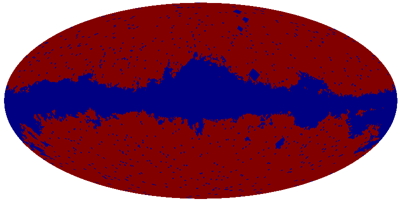
$R_{3}=6.9^{\prime}$	$R_{4}=10.6^{\prime}$	$R_{5}=16.3^{\prime}$
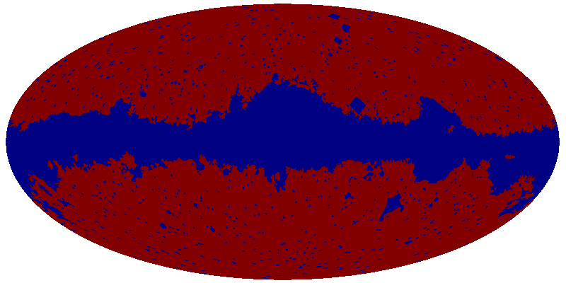
$R_{6}=14.9^{\prime}$	$R_{7}=38.3^{\prime}$	$R_{8}=58.7^{\prime}$
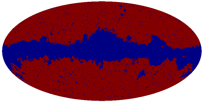
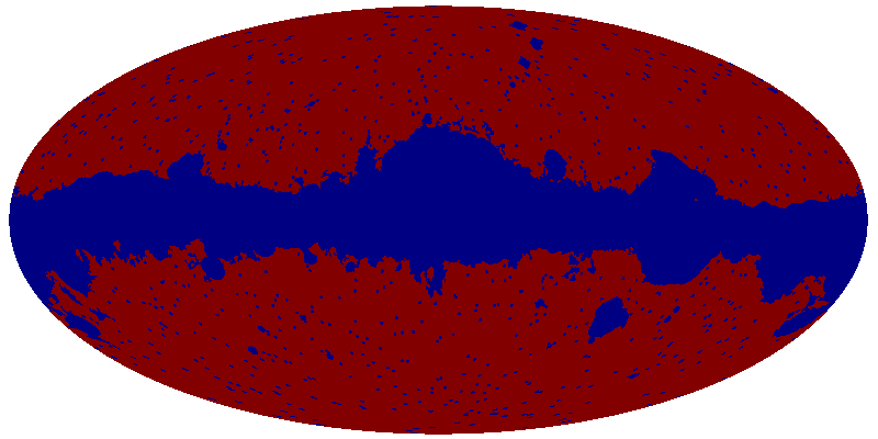
$R_{9}=90.1^{\prime}$	$R_{10}=138.3^{\prime}$	$R_{11}=212.3^{\prime}$
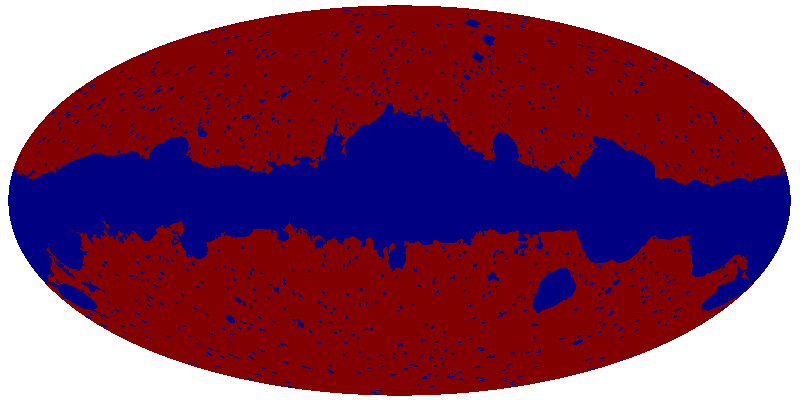
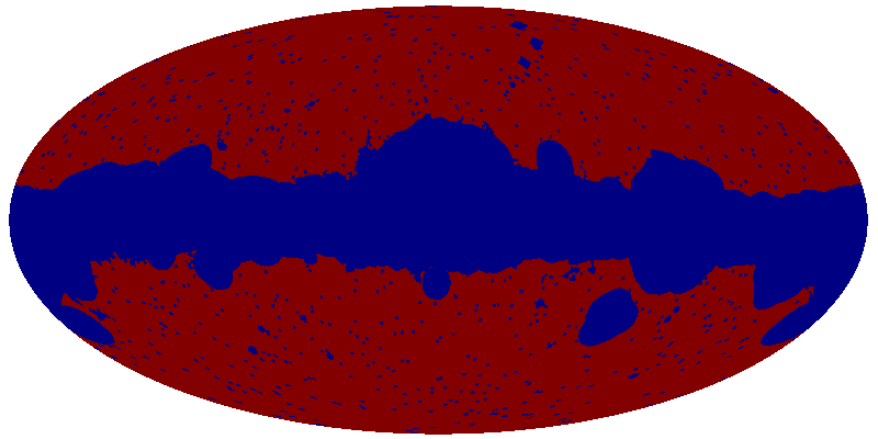
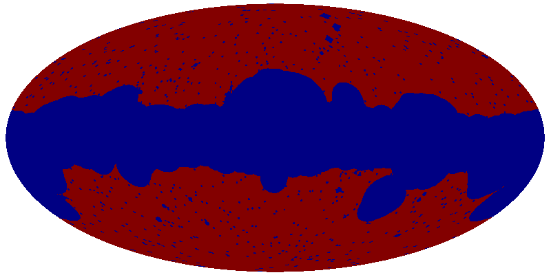
$R_{12}=325.8^{\prime}$	$R_{13}=500^{\prime}$	$R_{14}=767.3^{\prime}$

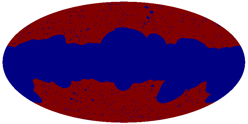
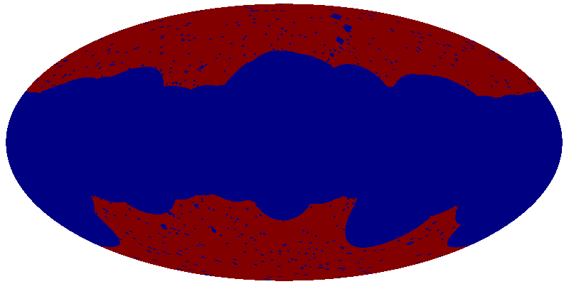
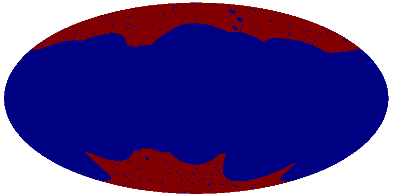
Figure 1: (Extended) masks appropriate for the analysis at each wavelet scale. The proportion of sky coverage for each mask is summarized in Table 2.

VI.2 Calculating the modal coefficients

As we have explained in Section II.2, to compute the late-time coefficients ($\bar{\alpha}^{Q}_{n}$) we first compute the primordial coefficients ($\alpha_{n}^{Q}$) for the shape $S_{\Phi}^{\text{(loc)}}$ defined in (11). For each triple $(p,r,s)$ which defines a basis function we compute $\ell^{2}=p^{2}+r^{2}+s^{2}$ and retain only the 80 modes with lowest $\ell$. This is sufficient to obtain a correlation of $\gtrsim 99\%$ for the usual bispectrum templates (local, constant, equilateral, orthogonal and flattened), except for the flattened model where we achieve $\sim 95\%$ correlation. This can be attributed to an inherent lack of smoothness of the template in the flattened limit, which makes the modal decomposition converge only slowly. We use the same number of modes to decompose the reduced angular bispectrum $b_{l_{1}l_{2}l_{3}}$. Later, we will verify that this is sufficient to ensure an accurate representation.

In order to calculate the transfer matrix $\Gamma_{pn}$ from primordial to late-time coefficients we first extract the transfer function from CAMB [25] and compute the line-of-sight projections $\tilde{q}_{p}^{(2)l}(x)$ and $\tilde{q}_{p}^{(-1)l}(x)$ defined in Eq. (21). We then compute $\tilde{\gamma}_{mn}(x)$ and $\bar{\gamma}_{mn}$ using Eqs. (40) and (42). Combining all these elements enables us to compute the transfer matrix from (43).

VI.3 Calculating the observed wavelets and modes

Our first task is to estimate the expectation value $V_{I}$ of each cubic wavelet statistic. To do so we simulate Gaussian spherical harmonic transforms with the variance for each multipole given by the angular temperature power spectrum, $C_{l}$. These are denoted $a_{lm}^{G}$. Using the prescription outlined in Section IV.2 we generate the simulated non-Gaussian multipoles, $a_{lm}^{B(n)}$, corresponding to the bispectrum basis function $b_{l_{1}l_{2}l_{3}}^{(n)}$ [defined in (36)]. The combination $a_{lm}=a_{lm}^{G}+a_{lm}^{B(n)}$ gives the simulated temperature map. The WMAP7 beam, $b_{l}$, and noise $n_{lm}$ can be incorporated via the transformation

$$a_{lm}\rightarrow\tilde{a}_{lm}=b_{l}a_{lm}+n_{lm}.$$ (53)

Using Eq. (26) we create simulated Gaussian and non-Gaussian wavelet maps for each scale and apply the appropriate masks. Then, for each map, the average in the unmasked region is subtracted. Finally we extract the cubic statistics $W^{G}_{I}$, $W^{B(n)}_{I}$ using (27). (Note here that the normalization coefficients for each cubic statistic, $\sigma_{i}^{2}$, are obtained using the assumption of isotropic noise. One should not be concerned, because these factors merely represent a normalization convention and cancel out in the estimator, Eq. (32).) With the fifteen wavelet scales used in this paper we obtain 680 cubic statistics. Expectation values for each of the 680 are computed by averaging over 300 simulations, after which we compute the change-of-basis matrix $V_{nI}$ using (48). We then compute a wavelet map of the real 7-year WMAP data, mask it, and extract cubic statistics $\tilde{W}_{I}$ in the same way.

In order to compute the $680\times 680$ covariance matrix $C_{IJ}$, we evaluate the expectation value $C_{IJ}=\langle\tilde{W}^{G}_{I}\tilde{W}^{G}_{J}\rangle-\langle\tilde{W}^{G}_{I}\rangle\langle\tilde{W}^{G}_{J}\rangle$ over $3\times 10^{4}$ simulations. The wavelet estimator (32) requires the inverse matrix $C_{IJ}^{-1}$, and once this has been obtained the quantities $\bar{\beta}_{n}^{Q}$ and $\overline{\gamma}_{nm}$ can be computed.

For each model under consideration we may obtain an estimate for the $f_{\mathrm{NL}}$ parameter, $\hat{f}_{\mathrm{NL}}^{b}$, and its expected (Fisher) variance, $\sigma^{2}_{F}(\hat{f}_{\mathrm{NL}}^{b})$, using (32) and (33), respectively. We also compute the variance of $\hat{f}_{\mathrm{NL}}^{b}$ from a suite of 100 simulations. Irrespective of whether the linear term (31) is subtracted, we recover the expected Fisher variance to high accuracy.

VI.4 Validation procedure

Gaussian validation. To ensure that our implementation is unbiased, we perform $4000$ Gaussian simulations. A critical ‘sanity’ check, described by Eq. (52), is to verify that the mean value $\langle\bar{\beta}^{R}_{n}\rangle$ for each $n$ is consistent with zero, within the standard error of the mean. (This is equal to the standard deviation divided by the square root of the number of simulations.) We plot the results in Fig. 2, from which we conclude that our methodology successfully passes this test. We have evaluated the wavelet-based estimator (51) for these simulations with the result

$$\langle\hat{f}_{\mathrm{NL}}\rangle=-0.3\pm 23.6.$$ (54)

Note that the standard deviation $23.6$ recovers the Fisher value obtained from (33), $\sigma_{F}(\hat{f}_{\rm{NL}})=23.6$, precisely. We have verified that neglecting the linear term (31) results in a minimal ($\lesssim 2\%$) difference in the standard deviation.

Non-Gaussian validation. We produce $100$ local simulations with $f_{\mathrm{NL}}^{\text{loc}}=100$, using the method described in [31]. For each of these simulations we extract the observed modes, $\bar{\beta}_{n}^{R}$. The critical sanity check (52) can now be carried out by comparing the theoretical expectation $\bar{\alpha}_{n}^{R}$ to each observed mode. In Figure 3 we show that this test is again satisfied within the error bars. The recovered value of $f_{\mathrm{NL}}$ is found to be

$$\langle\hat{f}_{\mathrm{NL}}\rangle=99.9\pm 2.5\,,$$ (55)

where the error bar quoted in this case is the standard error of the mean.

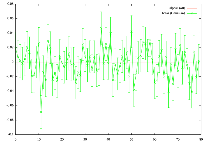
Figure 2: Mean of $\langle\bar{\beta}_{n}^{R}\rangle$ from $1000$ Gaussian simulations. To verify consistency of each mode with zero we plot the standard error of the mean (ie. the standard error divided by the square root of the number of simulations). Every mode is consistent with zero within two standard errors of the mean.

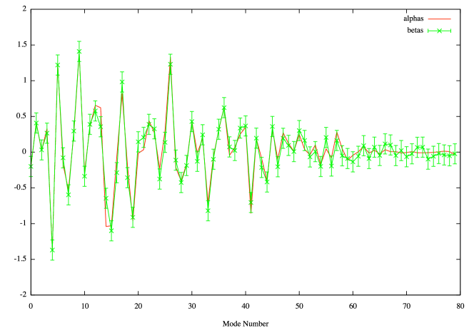
Figure 3: Comparison of the modal coefficients for the local shape, $\bar{\alpha}_{n}^{R}$, to the observed coefficients, $\bar{\beta}_{n}^{R}$. The observed coefficients are computed by simulating $100$ local maps with $f_{\mathrm{NL}}^{\text{loc}}=100$ as described in Ref. [31]. We plot the mean of these modes and the standard error of the mean. The ‘sanity’ check (52) is satisfied.

VII 7-year WMAP constraints

In this Section we use the methodology described in Section VI to obtain constraints on a selection of nearly scale-invariant models. To date, most bispectrum analyses have considered the local and equilateral models, owing to their physical significance and computational simplicity. We extend these to include the constant, orthogonal and flattened templates. In Ref. [11] these models were studied using modal methods and a bispectrum-based analysis. However, the wavelet-based approach adopted here yields a treatment which is closer to optimal. For example, in the case of local non-Gaussianity the error bar is reduced from $\Delta f_{\mathrm{NL}}=27.6$ to $\Delta f_{\mathrm{NL}}=23.6$. In Table 3 we compare our results with those of [11], highlighting the improvement in optimality achievable with the approach adopted in this paper. The comparison highlights the significant improvement over a standard modal-based approach, which, thus far, has been constrained in its scope, to using the same basis for the estimator as that used for the decomposition of the shape. This necessity may be avoided by employing the change of basis matrix, (48), with the modal technique used for the shape decomposition and wavelets being employed for extraction of the data in this work.

Shape	Current Paper	FLS [11]
$\displaystyle{\rm{Local}}$	$\displaystyle\,\,\,38.4\pm 23.6$	$\displaystyle 20.3\pm 27.6$
$\displaystyle{\rm{Constant}}$	$\displaystyle-10.1\pm 60.6$	$\displaystyle 30.5\pm 95.9$
$\displaystyle{\rm{Equilateral}}$	$\displaystyle-119.2\pm 123.6$	$\displaystyle\quad 1.9\pm 127.4$
$\displaystyle{\rm{DBI}}$	$\displaystyle-50.1\pm 104.2$	$\displaystyle\,\,\,17.1\pm 121.8$
$\displaystyle{\rm{Orthogonal}}$	$\displaystyle-173.2\pm 101.5$	$\displaystyle-51.4\pm 103.8$
$\displaystyle{\rm{Flattened}}$	$\displaystyle\quad\,6.6\pm 10.4$	$\displaystyle\quad 3.0\pm 10.9$

Table 3: Comparison of the WMAP$7$ constraints found in this work with those of Fergusson, Liguori and Shellard [11]. The improvement is achieved by employing a more optimal estimation method, allowed due to the freedom in making a different choice of basis to extract the data from that used to decomposed the theoretical shape.

VII.1 Local model

The local model is defined by a series expansion of the primordial gravitation potential, $\Phi$, in powers of an exactly Gaussian potential, $\Phi_{G}$. It gives [32]

$$\Phi({\bf x})=\Phi_{G}({\bf x})+f_{\mathrm{NL}}(\Phi_{G}({\bf x})^{2}-\langle\Phi_{G}({\bf x})^{2}\rangle)\,.$$ (56)

Neglecting scale dependence, the local model is an accurate match for the non-Gaussian contribution generated by interactions which operate on superhorizon scales. It generates a bispectrum given by (10). Examples of scenarios that may produce appreciable local non-Gaussianity include multifield inflation and curvaton scenarios. By construction the shape $S_{\Phi}^{\text{(loc)}}=1$ for this model. For a comprehensive review, see Chen [5] and references therein.

In Figure 5 we plot the primordial bispectrum shape. The dominant signal occurs in the corners of the triangle, corresponding to ‘squeezed’ configurations where one momentum is much smaller than the other two. When transferred to the CMB bispectrum, this (almost) scale-invariant shape is redistributed, resulting in the presence of peaks in the three-dimensional CMB bispectrum. However, the dominant signal remains along the edges of the tetrahedral domain, i.e. where one $l$ is much smaller than the other two.

In Figure 4, we compare the modal coefficients for the local model against the coefficients reconstructed from 7-year WMAP data. We also plot the cumulative sum $\sum_{n=0}^{N_{\text{max}}}\bar{\alpha}_{n}^{R}\bar{\beta}_{n}^{R}/\sum_{n=0}^{79}(\bar{\alpha}_{n}^{R})^{2}$ to establish that the estimator does converge with $80$ modes. Our final constraint on the amplitude of a local-type bispectrum is

$$f_{\mathrm{NL}}^{\text{loc}}=38.4\pm 23.6\quad\text{or}\quad F_{\mathrm{NL}}^{\text{loc}}=38.4\pm 23.6.$$ (57)

This result is competitive with the outcome of other wavelet-based analyses. For example, Donzelli et al. [17] quoted the constraint $f_{\mathrm{NL}}^{\text{loc}}=37.5\pm 22.3$. The small difference in our results may be explained by the use of a slightly different masking procedure, and (perhaps more importantly) because their analysis used data up to $l_{\text{max}}=1500$.

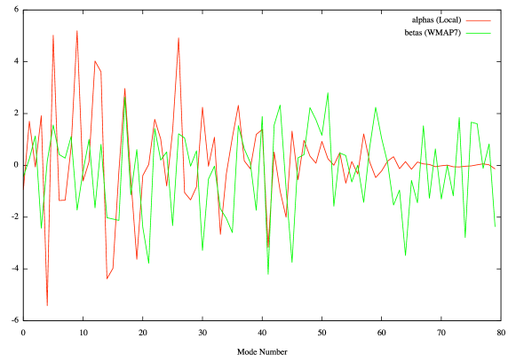
(a)

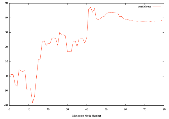
(b)

Figure 4: Modal comparison for local model.

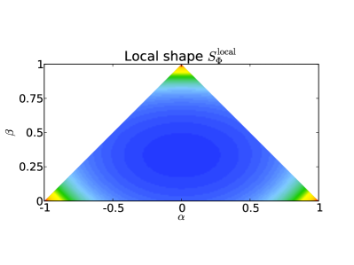
Figure 5: Canonical shape function (12) for the primordial local bispectrum. Due to the (almost) scale invariance of the shape it is only necessary to plot a particular slice. The parametrization $(\alpha,\beta)$ for each slice is chosen as described in Ref. [9]. In particular, $k_{1}/k_{t}=(1+\alpha+\beta)/4$, $k_{2}/k_{t}=(1-\alpha+\beta)/4$, $k_{3}/k_{t}=(1-\beta)/2$, where $k_{t}=\sum_{i}k_{i}$.

VII.2 Constant model

The constant model is simply $S_{\Phi}(k_{1},k_{2},k_{3})=1$. It is interesting because it produces a CMB bispectrum due completely to the transfer functions. One possible microphysical realization may occur during an epoch of quasi-single field inflation [33]. Our wavelet-based estimator yields the constraint

$$f_{\mathrm{NL}}^{\text{const}}=-10.1\pm 60.6\quad\text{or}\quad F_{\mathrm{NL}}^{\text{const}}=-3.9\pm 23.6.$$ (58)

VII.3 Equilateral and DBI models

Interactions which operate on superhorizon scales produce a local-shape bispectrum because causality requires the interaction to consist of a long-wavelength modulation of the background experienced by the short modes. This correlation between long and short modes is maximized in the squeezed limit.

In comparison, interactions which dominate on subhorizon scales typically produce no signal in the bispectrum, because subhorizon modes fluctuate incoherently and average to zero. An exception, where the initial state is non-empty, will be considered in Section VII.5 below. Neglecting that possibility, significant effects can be produced only near the epoch of horizon exit, where the fluctuations are beginning to behave coherently. In canonical slow-roll, single-field inflation the interference between horizon-scale fluctuations does not generate significant non-Gaussianity. However, with non-standard kinetic terms the amplitude of these effects may be enhanced [34, 35, 36]. Examples include DBI inflation and $k$-inflation.

The equilateral template is a separable approximation to the bispectrum produced by such models. It produces strong correlations for roughly equal $k$ because it is dominated by interference effects between wavenumbers which leave the horizon nearly simultaneously. We plot the shape function for the DBI model and the equilateral template in Fig. 6. They correspond to

$$B_{\Phi}^{\text{DBI}} =\frac{1}{(k_{1}k_{2}k_{3})^{3}(\sum_{i}k_{i})^{2}}\bigg{(}\sum_{i}k_{i}^{5}+\sum_{i\neq j}(2k_{i}^{4}k_{j}-3k_{i}^{3}k_{j}^{2})+\sum_{i\neq j\neq l}(k_{i}^{3}k_{j}k_{l}-4k_{i}^{2}k_{j}^{2}k_{l})\bigg{)}\,,$$ (59)

$$B_{\Phi}^{\text{eq}} =6\bigg{(}-\Big{[}P_{\Phi}(k_{1})P_{\Phi}(k_{2})+\text{2 perms}\Big{]}-2\Big{[}P_{\Phi}(k_{1})P_{\Phi}(k_{2})P_{\Phi}(k_{3})\Big{]}^{2/3}$$

$$\hskip 25.60747pt+\Big{[}P_{\Phi}^{1/3}(k_{1})P_{\Phi}^{2/3}(k_{2})P_{\Phi}(k_{3})+\text{5 perms}\Big{]}\bigg{)}\,.$$ (60)

Using (19) it can be shown that correlation between these shapes is $98\%$. The wavelet-based estimator gives the constraints

$$f_{\mathrm{NL}}^{\text{DBI}}=\,\,\,\ -50.1\pm 104.2\quad \text{or}\quad F_{\mathrm{NL}}^{\text{DBI}}=-11.4\pm 23.6\,,$$ (61)

$$f_{\mathrm{NL}}^{\text{eq}}=-119.2\pm 123.6\quad \text{or}\quad\,\,\,F_{\mathrm{NL}}^{\text{eq}}=-22.8\pm 23.6\,.$$ (62)

A variety of other bispectra dominated by interference effects near horizon-crossing, including the case of ghost inflation, were considered in Ref. [11]. All these models are highly correlated with the equilateral template and produce similar constraints.

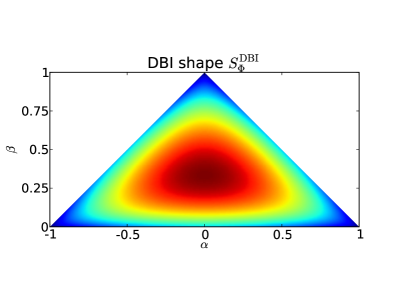
(a)

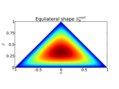
(b)

Figure 6: Canonical shape function, (12), for the primordial DBI bispectrum and equilateral bispectrum. The high degree of correlation between the two shapes, apparent from these plots, is $98\%$.

VII.4 Orthogonal Model

The orthogonal shape is a linear combination of the constant and equilateral shapes, corresponding to $S_{\Phi}^{\text{orth}}\propto S_{\Phi}^{\text{eq}}-(2/3)S_{\Phi}^{\text{const}}$ [8, 37]. It is roughly orthogonal to both the equilateral and local shapes. A separable template for its bispectrum is

$$B_{\Phi}^{\text{orth}} =6\bigg{(}3\Big{[}P_{\Phi}^{1/3}(k_{1})P_{\Phi}^{2/3}(k_{2})P_{\Phi}(k_{3})+\text{5 perms}\Big{]}-8\Big{[}P_{\Phi}(k_{1})P_{\Phi}(k_{2})P_{\Phi}(k_{3})\Big{]}^{2/3}-\frac{3}{2}B_{\Phi}^{\text{loc}}\bigg{)}\,.$$ (63)

It has been shown to arise in the DBI–Galileon model by Renaux-Petel [38]; see also Ref. [39]. We find the following constraint

$$f_{\mathrm{NL}}^{\text{orth}}=-173.2\pm 101.5\quad\text{or}\quad F_{\mathrm{NL}}^{\text{orth}}=-40.3\pm 23.6\,.$$ (64)

We note the consistency of this result with the constraint $f_{\mathrm{NL}}^{\text{orth}}=-159.8\pm 115.1$ obtained by Curto et al. [18].

VII.5 Flattened Model

If the initial state for fluctuations is not empty then it is possible to produce a bispectrum describing maximum correlation for ‘flattened’ configurations where, eg., $k_{1}\approx k_{2}+k_{3}$. The correlation arises because, with a nontrivial initial state, it is possible to find a ‘negative’ energy fluctuation with time dependence $\sim\mathrm{e}^{{-\mathrm{i}k_{1}t}}$ which interacts coherently with two positive energy fluctuations with time dependence $\sim\mathrm{e}^{{+\mathrm{i}k_{2}t}}$, $\mathrm{e}^{{+\mathrm{i}k_{3}t}}$. When $k_{1}\approx k_{2}+k_{3}$ the interaction is coherent over arbitrarily long times and does not average to zero in the subhorizon era.

Holman & Tolley studied a model in which the bispectrum produced by this effect was [40]

$$B_{\Phi}^{\text{flat}}=\frac{6}{39(k_{1}k_{2}k_{3})^{2}}\Bigg{[}\left(\frac{k_{1}^{2}+k_{2}^{2}-k_{3}^{2}}{k_{2}k_{3}}+\text{2 perms}\right)+12+8\left(\frac{k_{1}k_{2}+k_{1}k_{3}-k_{2}k_{3}}{(k_{2}+k_{3}-k_{1})^{2}}+\text{2 perms}\right)\Bigg{]}\,.$$ (65)

This is not separable. Its analysis is computationally intensive without a method such as modal decomposition, although alternatives approaches exist such as the use of Schwinger parameters [41].

Eq. (65) diverges in the flattened limit because the interaction continues over arbitrarily long times, and therefore becomes sensitive to whatever physics was operative throughout the inflationary era. By comparison, inflationary predictions using a vacuum initial state decouple from this unknown high-energy physics. To handle the divergence we parametrize our ignorance of the relevant physics using a cutoff [9], setting the bispectrum to zero for $k_{1}+k_{2}-k_{3}<Zk_{t}$ (or its permutations), where the perimeter $k_{t}=k_{1}+k_{2}+k_{3}$ was defined below Eq. (15). In this paper we take $Z=0.03$ as a fiducial value, although in a dedicated analysis $Z$ should be allowed to float. Furthermore, we smoothen the shape near the edges by employing a low pass (Gaussian) filter. With this choice, our constraints on the flattened model from the 7-year WMAP data are

$$f_{\mathrm{NL}}^{\text{flat}}=6.6\pm 10.4\quad\text{or}\quad F_{\mathrm{NL}}^{\text{flat}}=15\pm 23.6\,.$$ (66)

VIII Conclusions

In this paper we have developed a framework which combines partial-wave or ‘modal’ techniques with wavelet-based estimators for the CMB bispectrum.

Wavelet-based techniques are particularly efficient for CMB analysis because they take advantage of simultaneous localization on the temperature map in both scale and position. However, it is not straightforward to build a wavelet-based estimator for the amplitude of an arbitrary primordial bispectrum $B_{\Phi}$. Combining the wavelet-based methodology with the decomposition of $B_{\Phi}$ into a basis of partial-waves enables an efficient analysis—whether $B_{\Phi}$ is separable or not, provided only that it is a relatively smooth function of wavenumber.

Our framework has other advantages. Optimal bispectrum-based estimators are typically hampered by the need to invert a pixel-by-pixel covariance matrix of size $\sim 10^{6}\times 10^{6}$. Because the wavelet-by-wavelet covariance matrix is typically much smaller, of order $\sim 10^{3}\times 10^{3}$, the problem is numerically much more tractable. Despite this large gain in numerical efficiency there is comparatively little trade-off in optimality. Indeed, our final error bars are quite close to those achieved by the optimal pixel-by-pixel approach. In addition, due to their localization properties, wavelets have been shown to allow for accurate analysis of point-sources, foregrounds, and other systematics [19, 42]. Hence, integrating the partial-wave methodology with a wavelet-based analysis has the potential to reproduce the successes of both. The work presented in this paper generalizes the scope of wavelet-based estimation to allow for analysis of arbitrary primordial bispectra.

We have implemented our methodology for the 7-year WMAP data. Our constraints are competitive (to within $\sim 5-10\%$) with comparable constraints published elsewhere, and represent an improvement of up to $\sim 15\%$ in comparison with the bispectrum-based modal estimator of Ref. [11]. In any case there is much to be gained from implementing different estimators: they will be sensitive to different combinations of the data, including the underlying systematics.

In future work, we intend to study the efficacy of the method in more detail and pursue an extension to the trispectrum. (See also Refs. [21, 22].) Although our constraints show that the 7-year WMAP data are consistent with Gaussianity, we will shortly be presented with an improved data set from Planck. We hope that the techniques described in this paper can help to correctly categorize the source of any signal—whether of primordial origin, or a foreground.

References

- Maldacena [2003] J. M. Maldacena, JHEP 05, 013 (2003), arXiv:astro-ph/0210603 .
- Langlois and Vernizzi [2010] D. Langlois and F. Vernizzi, Classical and Quantum Gravity 27, 124007 (2010), arXiv:1003.3270 [astro-ph.CO] .
- Bartolo et al. [2004] N. Bartolo, E. Komatsu, S. Matarrese, and A. Riotto, Phys. Rept. 402, 103 (2004), arXiv:astro-ph/0406398 .
- Komatsu [2010] E. Komatsu, Classical and Quantum Gravity 27, 124010 (2010), arXiv:1003.6097 [astro-ph.CO] .
- Chen [2010] X. Chen, Advances in Astronomy 2010 (2010), 10.1155/2010/638979, arXiv:1002.1416 [astro-ph.CO] .
- Komatsu et al. [2011] E. Komatsu, K. M. Smith, J. Dunkley, C. L. Bennett, B. Gold, G. Hinshaw, N. Jarosik, D. Larson, M. R. Nolta, L. Page, D. N. Spergel, M. Halpern, R. S. Hill, A. Kogut, M. Limon, S. S. Meyer, N. Odegard, G. S. Tucker, J. L. Weiland, E. Wollack, and E. L. Wright, Astrophysical Journal, Supplement 192, 18 (2011), arXiv:1001.4538 [astro-ph.CO] .
- Babich [2005] D. Babich, Physical Review D 72, 043003 (2005), arXiv:astro-ph/0503375 .
- Smith et al. [2009] K. M. Smith, L. Senatore, and M. Zaldarriaga, Journal of Cosmology and Astroparticle Physics 0909, 006 (2009), arXiv:0901.2572 [astro-ph] .
- Fergusson et al. [2010a] J. R. Fergusson, M. Liguori, and E. P. S. Shellard, Physical Review D 82, 023502 (2010a), arXiv:0912.5516 [astro-ph.CO] .
- Fergusson and Shellard [2011] J. Fergusson and E. S. Shellard, ArXiv e-prints (2011), arXiv:1105.2791 [astro-ph.CO] .
- Fergusson et al. [2012] J. R. Fergusson, M. Liguori, and E. P. S. Shellard, Journal of Cosmology and Astroparticle Physics 12, 032 (2012), arXiv:1006.1642 [astro-ph.CO] .
- Cayon et al. [2001] L. Cayon, J. L. Sanz, E. Martinez-Gonzalez, A. J. Banday, F. Argueso, J. E. Gallegos, K. M. Gorski, and G. Hinshaw, Monthly Notices of the Royal Astronomical Society 326, 1243 (2001), arXiv:astro-ph/0105111 .
- Mukherjee and Wang [2004] P. Mukherjee and Y. Wang, Astrophysical Journal 613, 51 (2004), arXiv:astro-ph/0402602 .
- Baldi et al. [2006] P. Baldi, G. Kerkyacharian, D. Marinucci, and D. Picard, ArXiv Mathematics e-prints (2006), arXiv:math/0606599 .
- Pietrobon et al. [2006] D. Pietrobon, A. Balbi, and D. Marinucci, Physical Review D 74, 043524 (2006), arXiv:astro-ph/0606475 .
- Lan and Marinucci [2008] X. Lan and D. Marinucci, Electronic Journal of Statistics 2, 332 (2008), arXiv:0802.4020 .
- Donzelli et al. [2012] S. Donzelli, F. K. Hansen, M. Liguori, D. Marinucci, and S. Matarrese, Astrophysical Journal 755, 19 (2012), arXiv:1202.1478 [astro-ph.CO] .
- Curto et al. [2012] A. Curto, E. Martinez-Gonzalez, and R. B. Barreiro, Monthly Notices of the Royal Astronomical Society 426, 1361 (2012), arXiv:1111.3390 [astro-ph.CO] .
- Curto et al. [2009] A. Curto, E. Martinez-Gonzalez, P. Mukherjee, R. B. Barreiro, F. K. Hansen, M. Liguori, and S. Matarrese, Monthly Notices of the Royal Astronomical Society 393, 615 (2009), arXiv:0807.0231 .
- Funakoshi and Renaux-Petel [2013] H. Funakoshi and S. Renaux-Petel, Journal of Cosmology and Astroparticle Physics 2, 002 (2013), arXiv:1211.3086 [astro-ph.CO] .
- Regan et al. [2010] D. M. Regan, E. P. S. Shellard, and J. R. Fergusson, Physical Review D 82, 023520 (2010), arXiv:1004.2915 [astro-ph.CO] .
- Fergusson et al. [2010b] J. R. Fergusson, D. M. Regan, and E. P. S. Shellard, ArXiv e-prints (2010b), arXiv:1012.6039 [astro-ph.CO] .
- Fergusson and Shellard [2007] J. R. Fergusson and E. P. S. Shellard, Physical Review D76, 083523 (2007), arXiv:astro-ph/0612713 .
- Fergusson and Shellard [2009] J. R. Fergusson and E. P. S. Shellard, Physical Review D 80, 043510 (2009), arXiv:0812.3413 .
- Lewis et al. [2000] A. Lewis, A. Challinor, and A. Lasenby, Astrophys. J. 538, 473 (2000), arXiv:astro-ph/9911177 .
- Blas et al. [2011] D. Blas, J. Lesgourgues, and T. Tram, Journal of Cosmology and Astroparticle Physics 7, 034 (2011), arXiv:1104.2933 [astro-ph.CO] .
- Martinez-Gonzalez et al. [2002] E. Martinez-Gonzalez, J. E. Gallegos, F. Argüeso, L. Cayón, and J. L. Sanz, Monthly Notices of the Royal Astronomical Society 336, 22 (2002), arXiv:astro-ph/0111284 .
- Sanz et al. [2006] J. L. Sanz, D. Herranz, M. Lopez-Caniego, and F. Argueso, ArXiv Astrophysics e-prints (2006), arXiv:astro-ph/0609351 .
- Komatsu and Spergel [2001] E. Komatsu and D. N. Spergel, Physical Review D63, 063002 (2001), arXiv:astro-ph/0005036 .
- Gorski et al. [2005] K. M. Gorski et al., Astrophysical Journal 622, 759 (2005), arXiv:astro-ph/0409513 .
- Hanson et al. [2009] D. Hanson, K. M. Smith, A. Challinor, and M. Liguori, Physical Review D80, 083004 (2009), arXiv:0905.4732 [astro-ph.CO] .
- Salopek and Bond [1990] D. S. Salopek and J. R. Bond, Physical Review D 42, 3936 (1990).
- Chen and Wang [2010] X. Chen and Y. Wang, Physical Review D 81, 063511 (2010), arXiv:0909.0496 [astro-ph.CO] .
- Alishahiha et al. [2004] M. Alishahiha, E. Silverstein, and D. Tong, Physical Review D70, 123505 (2004), arXiv:hep-th/0404084 .
- Chen et al. [2007a] X. Chen, R. Easther, and E. A. Lim, Journal of Cosmology and Astroparticle Physics 0706, 023 (2007a), arXiv:astro-ph/0611645 .
- Chen et al. [2007b] X. Chen, M.-x. Huang, S. Kachru, and G. Shiu, Journal of Cosmology and Astroparticle Physics 0701, 002 (2007b), arXiv:hep-th/0605045 .
- Meerburg et al. [2009] P. D. Meerburg, J. P. van der Schaar, and P. S. Corasaniti, Journal of Cosmology and Astroparticle Physics 0905, 018 (2009), arXiv:0901.4044 [hep-th] .
- Renaux-Petel [2011] S. Renaux-Petel, Classical and Quantum Gravity 28, 249601 (2011), arXiv:1105.6366 [astro-ph.CO] .
- Ribeiro and Seery [2011] R. H. Ribeiro and D. Seery, Journal of Cosmology and Astroparticle Physics 10, 027 (2011), arXiv:1108.3839 [astro-ph.CO] .
- Holman and Tolley [2008] R. Holman and A. J. Tolley, Journal of Cosmology and Astroparticle Physics 0805, 001 (2008), arXiv:0710.1302 [hep-th] .
- Smith and Zaldarriaga [2011] K. M. Smith and M. Zaldarriaga, Monthly Notices of the Royal Astronomical Society 417, 2 (2011), arXiv:astro-ph/0612571 .
- McEwen et al. [2007] J. D. McEwen, P. Vielva, Y. Wiaux, R. B. Barreiro, L. Cayon, M. P. Hobson, A. N. Lasenby, E. Martinez-Gonzalez, and J. L. Sanz, Journal of Fourier Analysis and Applications 13, 495 (2007), arXiv:0704.3158 .