Smoothed quantile regression processes for binary response models.

Abstract

In this paper, we consider binary response models with linear quantile restrictions. Considerably generalizing previous research on this topic, our analysis focuses on an infinite collection of quantile estimators. We derive a uniform linearisation for the properly standardized empirical quantile process and discover some surprising differences with the setting of continuously observed responses. Moreover, we show that considering quantile processes provides an effective way of estimating binary choice probabilities without restrictive assumptions on the form of the link function, heteroskedasticity or the need for high dimensional non-parametric smoothing necessary for approaches available so far. A uniform linear representation and results on asymptotic normality are provided, and the connection to rearrangements is discussed.

1 Introduction

In various situations in daily life, individuals are faced with making a decision that can be described by a binary variable. Examples relevant to various fields of economics include the decision to participate in the labour market, to retire, to make a major purchase. From an econometric point of view, such decisions can be modelled by a binary response variable $Y=I\{Y^{*}\geq 0\}$ that depends on an unobserved continuous random variable $Y^{*}$ which summarizes an individual’s preferences. In the presence of covariates, say $W$, a natural question is: what can we infer about the distribution of the unobserved variable $Y^{*}$ conditional on $W$ from observations of i.i.d. replicates of $(Y,W)$? In a seminal paper, Manski, (1975) assumed that $Y^{*}=W^{T}\beta+\varepsilon$ where the ‘error’ $\varepsilon$ satisfies the conditional median restriction $P(\varepsilon\leq 0|W=w)=0.5$ and derived conditions on the distribution of $(\varepsilon,W)$ that imply identifiability of the coefficient vector $\beta$ up to scale. In later work, Manski, (1985) extended those results to general quantile restrictions of the form $P(\varepsilon\leq 0|W=w)=\tau$ for fixed $\tau\in(0,1)$. A more detailed discussion of identification issues was provided in Manski, (1988). Due to their importance in understanding binary decisions, binary choice models have ever since aroused a lot of interest and many estimation procedures have been proposed [see Cosslett, (1983), Horowitz, (1992), Powell et al., (1989), Ichimura, (1993), Klein and Spady, (1993), Coppejans, (2001), Kordas, (2006) and Khan, (2013) to name just a few].

A particularly challenging part of analysing binary response models lies in understanding the stochastic properties of corresponding estimation procedures. The asymptotic distribution of Manski’s estimator was derived in Kim and Pollard, (1990) under fairly general conditions, while a non-standard case was considered in Portnoy, (1998). In particular, Kim and Pollard, (1990) demonstrated that the convergence rate is $n^{-1/3}$ and that the limiting distribution is non-Gaussian. A different approach based on non-parametric smoothing that avoids some of the difficulties encountered by Manski’s estimator was taken by Horowitz, (1992). By smoothing the objective function, Horowitz, (1992) obtained both - better rates of convergence and a normal limiting distribution. However, note that the smoothness conditions on the underlying model are stronger than those of Kim and Pollard, (1990).

The approaches of Manski and Horowitz have in common that only estimators for the coefficient vector $\beta$ are provided. While those coefficients are of interest and can provide valuable structural information, their interpretation can be quite difficult since the scale of $\beta$ is not identifiable from the observations. On the other hand, the ‘binary choice probabilities’ $p_{w}:=P(Y=1|W=w)$ provide a much simpler and more straightforward interpretation.

Most of the available methods for estimating binary choice probabilities are of two basic types. The first and more thoroughly studied approach is to assume a model of the form $Y^{*}=W^{T}\beta+\varepsilon$ where the $\varepsilon$ is assumed to be either independent of $W$ [see Cosslett, (1983) and Coppejans, (2001)], or admit a very special kind of heteroskedasticity [Klein and Spady, (1993)]. Another popular approach has been to embed the problem into general estimation of single index models, see for example Powell et al., (1989) or Ichimura, (1993). Here, it is again necessary to assume independence between $\varepsilon$ and the covariate $W$.

While in the settings described above it is possible to obtain parametric rates of convergence for the coefficient vector $\beta$ and also construct estimators for choice probabilities, in many cases the assumptions on the underlying model structure seem too restrictive.

An alternative approach allowing for general forms of heteroskedasticity was recently investigated by Khan, (2013), who proved that under general smoothness conditions any binary response model with $Y^{*}=W^{T}\beta+\varepsilon$ is observationally equivalent to a Probit/Logit model with multiplicative heteroskedasticity, that is a model where $\varepsilon=\sigma_{0}(W)U$ with $U$ independent of $W$ and general scale function $\sigma_{0}$. Khan, (2013) also proposed to simultaneously estimate $\beta$ and the function $\sigma_{0}$ by a semi-parametric sieve approach. The resulting model allows one to obtain an estimator of the binary choice probabilities. While this idea is extremely interesting, it effectively requires estimation of a $d$-dimensional function in a non-parametric fashion. For the purpose of estimating $\beta$, the function $\sigma_{0}$ can be viewed as a nuisance parameter and its estimation does not have an impact on the rate at which $\beta$ is estimable. However, the binary choice probabilities explicitly depend on $\sigma_{0}$ and can thus only be estimated at the corresponding $d$-dimensional non-parametric rate. In settings where $d$ is moderately large this can be quite problematic.

In the classical setting where responses are observed completely, linear quantile regression models [see Koenker and Bassett, (1978)] have proved useful in providing a model that can incorporate general forms of heteroskedasticity and at the same time avoid non-parametric smoothing. In particular, by looking at a collection of quantile coefficients indexed by the quantile level $\tau$ it is possible to obtain a broad picture of the conditional distribution of the response given the covariates. The aim of the present paper is to carry this approach into the setting of binary response models. In contrast to existing methods, we can allow for rather general forms of heteroskedasticity and at the same time estimate binary choice probabilities without the need of non-parametrically estimating a $d$-dimensional function.

The ideas explored here are closely related to the work of Kordas, (2006). Yet, there are many important differences. First, in his theoretical investigations, Kordas, (2006) considered only a finite collection of quantile levels. The present paper aims at considering the quantile process. Contrary to the classical setting, and also contrary to the results suggested by the analysis in Kordas, (2006), we see that the asymptotic distribution is a white noise type process with limiting distributions corresponding to different quantile levels being independent. An intuitive explanation of this seemingly surprising fact along with rigorous theoretical results can be found in Section 2. We thus provide both a correction and considerable extension of the findings in Kordas, (2006).
Further, our results on the quantile process pave the way to obtaining an estimator for the conditional probabilities $p_{w}$ and derive its asymptotic representation. While a related idea was considered in Kordas, (2006), no theoretical justification of its validity was provided. Moreover, we are able to considerably relax the identifiability assumptions that were implicitly made there. Finally, we demonstrate that our ideas are closely related to the concept of rearrangement [see Dette et al., (2006) or Chernozhukov et al., (2010)] and provide new theoretical insights regarding certain properties of the rearrangement map that seem to be of independent interest.
The rest of the paper is organized as follows. In Section 2, we formally state the model and provide results on uniform consistency and a uniform linearisation of the binary response quantile process. All results hold uniformly over an infinite collection of quantiles $T$. In Section 3, we show how the results from Section 2 can be used to obtain estimators of choice probabilities. We elaborate on the connection of this approach to rearrangements. A uniform asymptotic representation for a properly rescaled version of the proposed estimators is provided and their joint asymptotic distribution is briefly discussed. Theoretical properties of the rearrangement operator are collected in Section 3.1. Section 4 contains comments on practical implementation of the proposed estimation procedures together with a small simulation study. All proofs are deferred to an appendix.

2 Estimating the coefficients

Before we proceed to state our results, let us briefly recall some basic facts about identification in binary response models and provide some intuition for the estimators of Manski, (1975) and Horowitz, (1992). Throughout the paper, we consider the following data-generating process

• Assume that we have n i.i.d. replicates, say $(Y_{i},W_{i})_{i=1,...,n}$, drawn from the distribution $(Y=I\{Y^{*}\geq 0\},W)$ with $Y^{*}$ denoting the unobserved variable of interest and $W$ denoting a vector of covariates. Further, denote by $q_{\tau}(w)$ the conditional quantile function of $Y^{*}$ given $W=w$. Assume that for $\tau\in T\subset(0,1)$ we have $q_{\tau}(w)=w^{T}\beta_{\tau}$ for some vectors $\beta_{\tau}\in\mathbb{R}^{d+1}$.

Observing that $I\{Y^{*}\geq 0\}=I\{aY^{*}\geq 0\}$ with $a>0$ arbitrary directly shows that the scale of the vector $\beta_{\tau}$ can not be identified from $(Y,W)$. The vector $\beta_{\tau}$ is identified up to scale if for example $\gamma\neq\beta_{\tau}$ implies that the distribution of $Y$ conditional on $W^{T}\beta_{\tau}>0$ differs from that conditional on $W^{T}\gamma>0$ on a sufficiently large set. More precisely, assume that the function $u\mapsto F_{Y^{*}|W}(w^{T}\beta_{\tau}+u|w)$ is strictly increasing for $u$ in a neighbourhood of zero and all $w\in\mbox{support(W)}$. In that case we have by the definition of the $\tau$’th quantile

$$P(Y=1|W=w)\left\{\begin{array}[]{cc}>1-\tau,&\mbox{if}\ w^{T}\beta_{\tau}>0\\ =1-\tau,&\mbox{if}\ w^{T}\beta_{\tau}=0\\ <1-\tau,&\mbox{if}\ w^{T}\beta_{\tau}<0.\end{array}\right.$$

This suggests that the expectation of $(Y-(1-\tau))$ conditional on $W=w$ is positive for $w^{T}\beta_{\tau}>0$ and negative for $w^{T}\beta_{\tau}<0$. We thus expect that under appropriate conditions the function

$$S_{\tau}(\beta):=\mathbb{E}\Big{[}(Y-(1-\tau))I\{W^{T}\beta\geq 0\}\Big{]}$$

should be maximal at $a\beta_{\tau}$ for any $a>0$. Consider a vector $\gamma\in\mathbb{R}^{d+1}$. Then

$$S_{\tau}(\gamma)-S_{\tau}(\beta_{\tau})=D_{1}(\gamma,\tau)+D_{2}(\gamma,\tau)$$

with

$$D_{1}(\gamma,\tau) := \mathbb{E}[(Y-(1-\tau))I\{W^{T}\gamma\geq 0>W^{T}\beta_{\tau}\}],$$

$$D_{2}(\gamma,\tau) := -\mathbb{E}[(Y-(1-\tau))I\{W^{T}\gamma<0\leq W^{T}\beta_{\tau}\}].$$

Note that both quantities are non-positive, and at least one of them being strictly negative is sufficient for inferring $\beta_{\tau}/\|\beta_{\tau}\|\neq\gamma/\|\gamma\|$ from the observable data for a fixed quantile $\tau\in T$. An overview and more detailed discussion of related results is provided in Chapter 4 of Horowitz, (2009). Assumptions ensuring identifiability for a collection of quantiles $\tau\in T$ are discussed below.

A common assumption [see e.g. Chapter 4 in Horowitz, (2009)] is that one component of $\beta_{\tau}$ is either constant or at least bounded away from zero. Without loss of generality, we assume that this holds for the first component of $\beta_{\tau}$. In order to simplify the notation of what follows, write the covariate $W$ in the form $W^{T}=(Z,X^{T})$ with $Z$ being the first component of $W$ and $X$ denoting the remaining components. Denote the supports of $X,Z,W$ by $\mathcal{X},\mathcal{Z},\mathcal{W}$, respectively. Define the empirical counterpart of $S_{\tau}$ by

$$\tilde{S}_{n,\tau}(\beta):=\frac{1}{n}\sum_{i=1}^{n}(Y_{i}-(1-\tau))I\{W^{T}_{i}\beta\geq 0\}$$

and consider a smoothed version

$$\hat{S}_{n,\tau}(\beta):=\frac{1}{n}\sum_{i=1}^{n}(Y_{i}-(1-\tau))\mathcal{K}\Big{(}\frac{W^{T}_{i}\beta}{h_{n}}\Big{)}$$

with $h_{n}$ denoting a bandwidth parameter and $\mathcal{K}(u):=\int_{-\infty}^{u}K(v)dv$ a smoothed version of the indicator function $I\{u\geq 0\}$. Following Horowitz, (2009), define the estimator $(\hat{s}_{\tau},\hat{b}_{\tau})$ through

$$(\hat{s}_{\tau},\hat{b}_{\tau})=\mbox{argmax}_{s=\pm 1,b\in B}\hat{S}_{n,\tau}((s,b^{T})^{T}),$$ (2.1)

where $B\subset\mathbb{R}^{d}$ is some fixed compact set not depending on $\tau$. Note that we do not impose $\hat{s}_{\tau}=\hat{s}_{\tau^{\prime}}$ in the estimation. In principle, this would be possible, but it would require us to consider several minimizations simultaneously and result in computational difficulties. Uniform consistency of $\hat{s}_{\tau}$ proved below implies that all values of $\hat{s}_{\tau}$ for different $\tau\in T$ will be equal with probability tending to one.

Remark 2.1

The proofs of all subsequent results implicitly rely on the fact that we know which coefficient stays away from zero and that the covariate corresponding to this particular coefficient has a ‘nice’ distribution conditional on all other covariates [see assumptions (F1), (D2) etc.]. This is in line with the approach of Horowitz, (1992) and Kordas, (2006) and makes sense in many practical examples. Results similar to the ones presented below might continue to hold if we use Manski’s normalization $\|\hat{\beta}\|=1$ instead of setting the ‘right’ component to $\pm 1$. However, the asymptotic representation would be somewhat more complicated. For this reason, we leave this interesting question to future research. $\hfill\blacksquare$

Remark 2.2

As pointed out by the Editor Prof. P.C.B. Phillips, neither the approach of Horowitz, (1992) nor Manski’s normalization $\|\beta_{\tau}\|=1$ work when the sub-vector of $\beta_{\tau}$ which does not include the intercept is the zero vector. In particular, this is the case when the vector of covariates $W$ and the latent variable $Y^{*}$ are independent. The latter model is observationally equivalent to any other model where $Y$ is independent of $W$. $\hfill\blacksquare$

Remark 2.3

Note that, due to the scaling, the estimator $\hat{b}_{\tau}$ defined above is an estimator of the re-scaled quantity $\bar{b}_{\tau}:=b_{\tau}/|\beta_{\tau,1}|$ where $b_{\tau}:=(\beta_{\tau,2},...,\beta_{\tau,d+1})^{T}$. When interpreting the estimator $\hat{b}_{\tau}$, this must be taken into account. In particular, $\hat{b}_{\tau}$ can not be interpreted as a classical quantile regression coefficient. The fact that we divide by $|\beta_{\tau,1}|$ also explains the reason behind assumption (A). Some comments on the practical choice of this normalization are given in Section 4. $\hfill\blacksquare$

In all of the subsequent developments we make the following basic assumption.

1. The coefficient $\beta_{\tau,1}$ satisfies $\inf_{\tau\in T}|\beta_{\tau,1}|>0$ and the coefficient $\beta_{\tau,1}$ has the same sign for all $\tau\in T$. In what follows, denote this sign by $s_{0}$.

In order to establish uniform consistency of the smoothed maximum score estimator, we need the following assumptions.

1. The function $\mathcal{K}$ is uniformly bounded and satisfies $\sup_{|v|\geq c}|\mathcal{K}(v)-I\{v\geq 0\}|\to 0$ as $c\to\infty$.

2. The conditional distribution function of $Z$ given $X$, say $F_{Z|X}$, is uniformly continuous uniformly over $x\in\mathcal{X}$, that is

   $$\sup_{x\in\mathcal{X}}\sup_{v\in\mathbb{R}}\sup_{|u|\leq\delta}|F_{Z|X}(v|x)-F_{Z|X}(v+u|x)|\to 0\quad\mbox{as}\quad\delta\to 0.$$

3. For any fixed $\tau\in T$, $\bar{\beta}_{\tau}=(s_{0},\bar{b}_{\tau}^{T})^{T}$ is the unique minimizer of $S_{\tau}(\beta)$ on $\{-1,1\}\times B$ and additionally

   $$d(\varepsilon):=\inf_{\tau\in T}\inf_{\|\beta-\bar{\beta}_{\tau}\|\geq\varepsilon,|\beta_{1}|=1}|S_{\tau}(\beta)-S_{\tau}(\bar{\beta}_{\tau})|>0\quad\forall\varepsilon>0.$$

In order to intuitively understand the meaning of condition (D1) above, note that conditions (K1) and (F1) imply that $\hat{S}_{n,\tau}(\beta)\to S_{\tau}(\beta)$ uniformly in $\tau,\beta$. Condition (D1) essentially requires that the maximum of $S_{\tau}(\beta)$ is ‘well separated’ uniformly in $\tau$, which allows to obtain uniform consistency of a sequence of maximizers of any function that uniformly converges to $S_{\tau}$. Next, we give a simple condition on densities and distributions which implies (D1). This condition is inspired by the approach taken in Manski, (1985); Horowitz, (1992).

• The support of the distribution of $X$ is not contained in any proper linear subspace of $\mathbb{R}^{d}$. Additionally, the conditional density $f_{Z|X}(\cdot|x)$ of $Z$ given $X=x$ exists for all $x\in\mathcal{X}$ and $\inf_{x\in\mathcal{X}}\inf_{z\in[-D,D]}f_{Z|X}(z|x)>0$ for some $D>\sup_{b\in B,x\in\mathcal{X}}|b^{T}x|$.

The fact that (D1) follows from (A), (M) and (S) is proved in the appendix.

Lemma 2.4

Under assumptions (M), (K1), (D1), (F1) let $h_{n}\to 0$. Then the estimator $(\hat{s},\hat{b}_{\tau})$ is weakly uniformly consistent, that is

$$\sup_{\tau\in T}\|(\hat{s}_{\tau},\hat{b}_{\tau})-(s_{0},\bar{b}_{\tau})\|=o_{P}(1).$$

The next collection of assumptions is sufficient for deriving a uniform linearization for $\hat{b}_{\tau}.$ Assume that there exist $\eta>0,k_{0}\geq 2$ such that the following conditions hold.

1. The function $\mathcal{K}$ is two times continuously differentiable and its second derivative is uniformly Hölder continuous of order $\gamma>0$, that is it satisfies

   $$\sup_{|x-y|\leq\delta}|\mathcal{K}^{\prime\prime}(x)-\mathcal{K}^{\prime\prime}(y)|\leq C_{K}|x-y|^{\gamma}.$$

   Denote the derivative of $\mathcal{K}$ by $K$. Assume that $K,K^{\prime}$ are uniformly bounded, that $\int|v^{2}K^{\prime}(v)|dv<\infty,\int|K^{\prime}(v)|^{2}dv<\infty$, and that additionally $\alpha_{n}:=h_{n}^{-1}\int_{|vh_{n}|>\eta}|K^{\prime}(v)|dv=o(1)$.

2. Assume that $\int|v^{k_{0}}K(v)|<\infty$, $\int v^{j}K(v)dv=0$ for $1\leq j<k_{0}$, $\int_{|vh_{n}|>\eta}|K(v)|dv=o(h_{n}^{k_{0}})$ and that $\sup_{|a|>x}|K(a)|=o(x^{-1})$ as $x\to\infty$.

3. The bandwidth $h_{n}$ satisfies $h_{n}=o(1)$ and additionally $(nh_{n}^{3})^{-1/2}(\log n)^{2}=o(1)$.

4. The distribution of $X$ (denoted by $P_{X}$ from now on) has bounded support $\mathcal{X}$ and the matrix $E[WW^{T}]$ exists and is positive definite. For almost every $x\in\mathcal{X}$, the covariate $Z$ has a conditional density $f_{Z|X}(\cdot|x)$ and

   $$\inf_{\tau\in T}\inf_{x\in\mathcal{X}}f_{Z|X}(-s_{0}x^{T}\bar{b}_{\tau}|x)>0.$$

5. For any vector $b$ with $\|b-\bar{b}_{\tau}\|\leq\eta$ the two functions $u\mapsto f_{Z|X}(s_{0}(-x^{T}b+u)|x)$ and $u\mapsto F_{Y^{*}|X,Z}(0|x,s_{0}(-x^{T}b+u))$ are two times continuously differentiable at every $u$ with $|u|\leq\eta$ for almost every $x\in\mathcal{X}$ and the first and second derivatives are uniformly bounded [uniformly over $x\in\mathcal{X}$,$\tau\in T$].

6. The function $u\mapsto f_{Z|X}(s_{0}(-x^{T}\bar{b}_{\tau}+u)|x)$ is $k_{0}-1$ times continuously differentiable for every $x\in\mathcal{X}$ at every $\tau\in T$ and $u$ with $|u|\leq\eta$. All derivatives, say $\partial_{u}^{k}f_{Z|X}(s_{0}(-x^{T}\bar{b}_{\tau}+u)|x)$, are uniformly bounded and satisfy: for all $\varepsilon>0$ there exists $\delta>0$ such that

   $$\sup_{|u|\leq\eta,|u^{\prime}|\leq\eta,|u-u^{\prime}|\leq\delta}\sup_{\tau\in T}\sup_{x\in\mathcal{X}}\Big{|}\partial_{u}^{k}f_{Z|X}(s_{0}(-x^{T}\bar{b}_{\tau}+u)|x)-\partial_{u}^{k}f_{Z|X}(s_{0}(-x^{T}\bar{b}_{\tau}+u^{\prime})|x)\Big{|}\leq\varepsilon.$$

   The function $u\mapsto F_{Y^{*}|X,Z}(0|x,s_{0}(-x^{T}\bar{b}_{\tau}+u))$ is $k_{0}$ times continuously differentiable at every $\tau\in T$ and $u$ with $|u|\leq\eta$ at almost every $x\in\mathcal{X}$ and all derivatives, say $\partial_{u}^{k}F_{Y^{*}|X,Z}(0|x,s_{0}(-x^{T}\bar{b}_{\tau}+u))$, are uniformly bounded and satisfy: for all $\varepsilon>0$ there exists $\delta>0$ such that

   $$\sup_{|u|\leq\eta,|u^{\prime}|\leq\eta,|u-u^{\prime}|\leq\delta}\sup_{\tau\in T}\sup_{x\in\mathcal{X}}\Big{|}\partial_{u}^{k}F_{Y^{*}|X,Z}(0|x,s_{0}(-x^{T}\bar{b}_{\tau}+u))-\partial_{u}^{k}F_{Y^{*}|X,Z}(0|x,s_{0}(-x^{T}\bar{b}_{\tau}+u^{\prime}))\Big{|}\leq\varepsilon.$$

7. The map $\tau\mapsto\beta_{\tau}$ is Hölder continuous of order $\gamma>0$ uniformly on $T$, that is we have $\sup_{\tau,\tau^{\prime}\in T,|\tau-\tau^{\prime}|\leq\delta}\|\beta_{\tau}-\beta_{\tau^{\prime}}\|\leq C\delta^{\gamma}$ for some constant $C<\infty$ and all $\delta>0$.

8. For every $w\in\mathcal{W}$, the random variable $Y^{*}$ has a conditional density $f_{Y^{*}|W}$ conditional on $W=w$. Moreover,

   $$\inf_{\tau\in T}\inf_{x\in\mathcal{X}}f_{Y^{*}|X,Z}(0|x,-s_{0}x^{T}\bar{b}_{\tau})>0,\quad\sup_{\tau\in T}\sup_{x\in\mathcal{X}}f_{Y^{*}|X,Z}(0|x,-s_{0}x^{T}\bar{b}_{\tau})<\infty.$$

9. The function $(y,w)\mapsto f_{Y^{*}|W}(y|w)$ is uniformly bounded on $\mathbb{R}\times\mathcal{W}$, i.e.

   $$\sup_{y\in\mathbb{R},w\in\mathcal{W}}f_{Y^{*}|W}(y|w)<\infty,$$

   and uniformly continuous on the set $\{|y|\leq\eta\}\times\mathcal{W}$.

The conditions on the kernel function $K$ are standard in the binary response setting and were for example considered in Horowitz, (2009) and Kordas, (2006). Assumptions (D2)-(D4) are uniform versions of the conditions in Horowitz, (1992) and are used to obtain results holding uniformly in an infinite collection of quantiles. Condition (D5) is used to obtain a rate in the uniform representation below. In particular, (D5) will follow with $\gamma=1$ if there exists a set $\mathcal{W}_{0}\subset\mathcal{W}$ such that the matrix $\mathbb{E}[WW^{T}I_{\{W\in\mathcal{W}_{0}\}}]$ is positive definite and $\inf_{w\in\mathcal{W}_{0},\tau\in T}f_{Y^{*}|W}(w^{T}\beta_{\tau}|w)>0$. Conditions (D6) and (Q) place mild restrictions on the conditional density of $Y^{*}$ given $W=w$. This kind of assumption is standard in classical quantile regression.

Theorem 2.5

Under assumptions (A), (B), (M), (D1)-(D5), (F1), (K1)-(K3), (Q) we have

$$Q_{0}(\tau)(\hat{b}_{\tau}-\bar{b}_{\tau})=-\tilde{T}_{n}(s_{0},\bar{b}_{\tau},\tau)+R_{n}(\tau),$$ (2.2)

where

$$Q_{0}(\tau) := |\beta_{\tau,1}|\int f_{Z|X}(-s_{0}x^{T}\bar{b}_{\tau}|x)f_{Y^{*}|X,Z}(0|x,-s_{0}x^{T}\bar{b}_{\tau})xx^{T}dP_{X}(x),$$

$$\tilde{T}_{n}(s,b,\tau) := \frac{\partial\tilde{S}_{n,\tau}((s,b^{T})^{T})}{\partial b}=\frac{1}{nh_{n}}\sum_{i=1}^{n}(Y_{i}-(1-\tau))X_{i}K\Big{(}\frac{X_{i}^{T}b+sZ_{i}}{h_{n}}\Big{)},$$

$$\sup_{\tau\in T}\|R_{n}(\tau)\| = O_{P}(\kappa_{n}):=O_{P}\Big{(}(h_{n}^{k_{0}}+(nh_{n})^{-1/2}\log n)((nh_{n}^{3})^{-1/2}\log n+h_{n}+\alpha_{n})\Big{)},$$

and $\alpha_{n}$ is defined in assumption (K2). In particular, $\kappa_{n}=o(h_{n}^{k_{0}}+(nh_{n})^{-1/2})$ and thus $R_{n}$ is negligible compared to $\tilde{T}_{n}(s_{0},\bar{b}_{\tau},\tau)$.
Now assume that additionally condition (D6) holds and that $h_{n}^{2{k_{0}}}=o((nh_{n})^{-1/2})$. Then, for any finite collection $\tau_{1},...,\tau_{K}\in T$, we obtain

$$\Big{(}\sqrt{nh_{n}}\Big{(}\hat{b}_{\tau_{j}}-\bar{b}_{\tau_{j}}-T_{n}(s_{0},\bar{b}_{\tau_{j}},\tau_{j})\Big{)}\Big{)}_{j=1,...,K}\stackrel{{\scriptstyle\mathcal{D}}}{{\rightarrow}}\Big{(}(Q_{0}(\tau_{j}))^{-1}M_{\tau_{j}}\Big{)}_{j=1,...,K},$$ (2.3)

where $\stackrel{{\scriptstyle\mathcal{D}}}{{\rightarrow}}$ denotes convergence in distribution,

$$T_{n}(s,b,\tau) := \frac{h_{n}^{k_{0}}}{{k_{0}}!}\int v^{k_{0}}K(v)dv\int g_{k}(s,b,x)xdP_{X}(x),$$

$$g_{j}(s,b,x) := \frac{\partial^{j}}{\partial u^{j}}\Big{(}(\tau-F_{Y^{*}|X,Z}(0|x,s(-x^{T}b+u)))f_{Z|X}(s(-x^{T}b+u)|x)\Big{)}\Big{|}_{u=0},$$

$M_{\tau_{i}},M_{\tau_{j}}$ are independent for $j\neq i$ and

$$M_{\tau}\sim\mathcal{N}(0,\Sigma_{\tau})$$

where

$$\Sigma_{\tau}:=\tau(1-\tau)\int K^{2}(u)du\int xx^{T}f_{Z|X}(-s_{0}x^{T}\bar{b}_{\tau}|x)dP_{X}(x).$$

Compared to the results available in the literature [e.g. in Kordas, (2006) and Horowitz, (2009)], the preceding theorem provides two important new insights. To the best of our knowledge, it is the first time that the estimator is simultaneously considered at an infinite collection of quantiles. Equally importantly, it demonstrates that the joint asymptotic distribution of several quantiles differs substantially from what both intuition and results in Kordas, (2006) seem to suggest.

Remark 2.6

In contrast to the setting when the response $Y^{*}$ is directly observed, the properly normalized quantile process at different quantile levels converges to independent random variables. An intuitive explanation for this surprising fact can be obtained from the asymptotic linearization in (2.2). For simplicity, assume that the kernel $K$ has compact support, say $[-1,1]$. To bound the covariance between the leading terms in the linearization of $\hat{b}_{\tau_{1}},\hat{b}_{\tau_{2}}$, begin by observing that under the assumptions of Theorem 2.5 we have for any $1\leq j,j^{\prime}\leq d$ [see equation (5.11) in the Appendix for a proof]

$$\Big{|}\mbox{Cov}\Big{(}\sqrt{nh_{n}}(\tilde{T}_{n}(s_{0},\bar{b}_{\tau_{1}},{\tau_{1}}))_{j},\sqrt{nh_{n}}(\tilde{T}_{n}(s_{0},\bar{b}_{\tau_{2}},{\tau_{2}}))_{j^{\prime}}\Big{)}\Big{|}$$

$$\leq \frac{C}{h_{n}}\int\int\Big{|}K\Big{(}\frac{x^{T}\bar{b}_{\tau_{1}}+s_{0}z}{h_{n}}\Big{)}K\Big{(}\frac{x^{T}\bar{b}_{\tau_{2}}+s_{0}z}{h_{n}}\Big{)}\Big{|}f_{Z|X}(z|x)dzdP_{X}(x)+O(h_{n}).$$

Noting that $x^{T}\bar{b}_{\tau}+s_{0}z=w^{T}\beta_{\tau}/|\beta_{\tau,1}|$ with $w=(z,x)$, we find that $K\Big{(}\frac{x^{T}\bar{b}_{\tau_{1}}+s_{0}z}{h_{n}}\Big{)}K\Big{(}\frac{x^{T}\bar{b}_{\tau_{2}}+s_{0}z}{h_{n}}\Big{)}\neq 0$ if and only if $|w^{T}\beta_{\tau_{k}}|\leq h_{n}|\beta_{\tau_{k},1}|,k=1,2$, which implies $|w^{T}\beta_{\tau_{1}}-w^{T}\beta_{\tau_{2}}|\leq h_{n}(|\beta_{\tau_{1},1}|+|\beta_{\tau_{2},1}|)$. Next, note that $w^{T}\beta_{\tau}=F_{Y^{*}|W}^{-1}(\tau|w)$. Under assumption (D6) it follows that

$$|F_{Y^{*}|W}(y_{1}|w)-F_{Y^{*}|W}(y_{2}|w)|\leq|y_{1}-y_{2}|\sup_{(y,w)\in\mathbb{R}\times\mathcal{W}}f_{Y^{*}|W}(y|w)=:f_{\infty}|y_{1}-y_{2}|$$

for any $w\in\mathcal{W}$. Substituting $y_{k}=F_{Y^{*}|W}^{-1}(\tau|w)=w^{T}\beta_{\tau_{k}},k=1,2$ we find that $|w^{T}(\beta_{\tau_{1}}-\beta_{\tau_{2}})|\geq f_{\infty}^{-1}|{\tau_{1}}-{\tau_{2}}|$ for any $w\in\mathcal{W}$. Hence for $\tau_{1}\neq\tau_{2}$ the set $\{w\in\mathcal{W}:|w^{T}\beta_{\tau_{k}}|\leq h_{n}|\beta_{\tau_{k},1}|\mbox{ for }k=1,2\}$ will be empty for $h_{n}$ sufficiently small and asymptotic independence follows since the integral in the inequality above is identically zero as soon as $h_{n}$ is sufficiently small.

Intuitively speaking, all observations that have a non-zero contribution to $\tilde{T}_{n}(s_{0},\bar{b}_{\tau},\tau)$ will need to satisfy $|W_{i}^{T}\beta_{\tau}|\leq h_{n}|\beta_{\tau,1}|$. In particular, letting $h_{n}\to 0$ implies that asymptotically, for different values of $\tau$, disjoint sets of observations will be driving the distribution of $T_{n}$. Similar phenomena can be observed in other settings that include non-parametric smoothing, a classical example being density estimation.

Note that regarding this particular point the paper of Kordas, (2006) contained a mistake. More precisely, Kordas, (2006) claimed that the asymptotic distributions corresponding to different quantiles have a non-trivial covariance which is not the case. $\hfill\blacksquare$

Remark 2.7

As pointed out by a referee, asymptotic independence at different quantile levels does not occur in the setting of kernel-smoothing based quantile regression–see for instance Chaudhuri, (1991). This is due to the fact that the leading term in the Bahadur representation for kernel-based quantile regression typically is of the form $n^{-1}M_{n}(\tau,x)\sum_{i}W_{n}(X_{i},x)(I\{Y_{i}\leq q_{\tau}\}-\tau)$. The weights $W_{n}(X_{i},x)$ can often be bounded by $C_{n}I\{|X_{i}-x|\leq h_{n}\}$ for some constants $C_{n}$ and a bandwidth parameter $h_{n}\to 0$. However, the weights do not depend on $\tau$ so that for the same covariates but different quantiles the leading term is determined by the same set of observations. In contrast to that, the leading term in the present setting is $-(Q_{0}(\tau))^{-1}\frac{1}{nh_{n}}\sum_{i=1}^{n}(Y_{i}-(1-\tau))X_{i}K\Big{(}\frac{X_{i}^{T}\bar{b}_{\tau}+s_{0}Z_{i}}{h_{n}}\Big{)}$. Here, the quantile index $\tau$ appears in the kernel $K\Big{(}\frac{X_{i}^{T}\bar{b}_{\tau}+sZ_{i}}{h_{n}}\Big{)}$, and thus the quantile index also determines the set of observations which contribute to the asymptotic distribution of $\hat{\beta}_{\tau}$. This makes estimators at different quantiles asymptotically independent. $\hfill\blacksquare$

The findings in Theorem 2.5 imply that there can be no weak convergence of the normalized process $\Big{(}\sqrt{nh_{n}}\Big{(}\hat{b}_{\tau}-\bar{b}_{\tau}-T_{n}(s_{0},\bar{b}_{\tau},\tau)\Big{)}\Big{)}_{\tau\in T}$ in a reasonable functional sense since the candidate ‘limiting process’ has a ‘white noise’ structure and is not tight. This will present an additional challenge for the analysis of estimators for binary choice probabilities constructed in Section 3.

Before proceeding to the estimation of conditional (choice) probabilities, we briefly comment on potential extensions of the findings in this section to parametric conditional quantile models that are not necessarily linear.

Remark 2.8

As pointed out by the associate editor and a referee, it is natural to wonder if the methods discussed above can be extended to parametric non-linear models. The ideas discussed in this section can be generalized to settings where the latent variables $Y^{*}$ have conditional quantile functions of the form

$$q_{\tau}(x,z)=s_{0}z+h(x,b_{\tau}),\quad\tau\in T$$ (2.4)

for a set $T\subset(0,1)$, a parametric function $h$ that depends on the parameter $b$ which can vary with $\tau$ and where $s_{0}\in\{-1,1\}$ is independent of $\tau$. Note that any model where the conditional quantile functions of the latent variable $Y^{*}$ are of the form

$$q_{\tau}(x,z)=\beta_{\tau,1}z+\tilde{h}(x,\gamma_{\tau}),\quad\tau\in T$$ (2.5)

with $\beta_{\tau,1}$ bounded away from zero uniformly on $T$ is observationally equivalent to a model where $q_{\tau}(x,z)=sgn(\beta_{\tau,1})z+\tilde{h}(x,\gamma_{\tau})/|\beta_{\tau,1}|$ [with $sgn(a)$ denoting the sign of $a$]. Thus the model specification in (2.4) incorporates all models of the form (2.5), after re-parametrization. A generalization to other parametric models that do not have this simple additive structure seems possible, but developing the corresponding asymptotic results would require an approach that is different from the one in the present paper.

Estimators of the parameters in model (2.4) can now be constructed in a similar fashion as in the linear case. More precisely, it seems natural to define

$$(\hat{s}_{\tau},\hat{b}_{\tau})=\mbox{argmax}_{s=\pm 1,b\in B}\hat{S}_{n,\tau}(s,b)$$ (2.6)

where $B\subset\mathbb{R}^{p}$ is a compact set and

$$\hat{S}_{n,\tau}(s,b):=\frac{1}{n}\sum_{i=1}^{n}(Y_{i}-(1-\tau))\mathcal{K}\Big{(}\frac{sZ_{i}+h(X_{i},b))}{h_{n}}\Big{)}.$$

Under appropriate conditions on the parametrization and conditional distributions, the consistency results from Lemma 2.4 and asymptotic linearization from Theorem 2.5 can be generalized to the estimation of non-linear coefficients. Details are omitted for the sake of brevity. $\hfill\blacksquare$

3 Estimating conditional probabilities

Partly due to the lack of complete identification, the coefficients estimated in the preceding section might be hard to interpret. A more tractable quantity is given by the conditional probability $p_{w}:=P(Y=1|W=w)$. One possible way to estimate this probability is local averaging. However, due to the curse of dimensionality, this becomes impractical if the dimension of $W$ exceeds 2 or 3. An alternative is to assume that the linear model $q_{\tau}(w)=w^{T}\beta_{\tau}$ holds for all $\tau\in T\subset(0,1)$. By definition of $Y=I\{Y^{*}\geq 0\}$, the existence of $\tau_{w}\in T$ with $w^{T}\beta_{\tau_{w}}=0$ implies that $p_{w}=1-\tau_{w}$. Since the quantile function of $Y^{*}$ is given by $w^{T}\beta_{\tau}$ we obtain $P(Y^{*}\leq 0|W=w)=w^{T}\beta_{\tau_{w}}$. By definition of the quantile function and the assumptions on $Y^{*}$, $\tau<\tau_{w}\Leftrightarrow w^{T}\beta_{\tau}<w^{T}\beta_{\tau_{w}}$. This implies the equality $\tau_{w}=\int_{0}^{1}I\{w^{T}\beta_{\tau}\leq 0\}d\tau$. In particular, we have for any $(a,b)\subset T$ with $a<\tau_{w}<b$

$$p_{w}=1-\tau_{w}=\int_{0}^{1}I\{w^{T}\beta_{\tau}\geq 0\}d\tau=1-b+\int_{a}^{b}I\{w^{T}\beta_{\tau}\geq 0\}d\tau=1-b+\int_{a}^{b}I\{w^{T}\bar{\beta}_{\tau}\geq 0\}d\tau,$$

where the last equality follows since $w^{T}\beta_{\tau}=|\beta_{\tau,1}|w^{T}\bar{\beta}_{\tau}$ for all $w$ and $\tau$. This suggests to estimate $p_{w}$ by replacing $\beta_{\tau}$ in the above representation with the estimator $\hat{\beta}_{\tau}$ from the preceding section after choosing $(a,b)$ in some sensible manner. A similar representation was considered by Kordas, (2006) with $a=0,b=1$. The fact that $\hat{\beta}$ is an estimator of the re-scaled version $\bar{\beta}_{\tau}$ is not important here since multiplication by a positive number does not affect the inequality $w^{T}\beta_{\tau}\geq 0$. From here on, define

$$\hat{p}_{w}(a,b):=1-b+\int_{a}^{b}I\{w^{T}\hat{\beta}_{\tau}\geq 0\}d\tau.$$ (3.1)

From the definition of $\hat{p}_{w}(a,b)$, it is not difficult to show [using Lemma 2.4] that under (A), (K1), (F1) and (D1), (Q) holding for $T=[a,b]$ we have

$$\hat{p}_{w}(a,b)\stackrel{{\scriptstyle P}}{{\rightarrow}}\left\{\begin{array}[]{cl}1-a,&\mbox{if}\ p_{w}\geq 1-a,\\ p_{w},&\mbox{if}\ p_{w}\in(1-b,1-a),\\ 1-b,&\mbox{if}\ p_{w}\leq 1-b.\end{array}\right.$$ (3.2)

Under the same assumptions, the definition of $\hat{p}_{w}(a,b)$ implies that, with probability tending to one, $\hat{p}_{w}(a,b)=\hat{p}_{w}(a^{\prime},b^{\prime})$ as long as $a<\tau_{w}<b$ and $a^{\prime}<\tau_{w}<b^{\prime}$. This suggests that, from an asymptotic point of view, the choice of $a,b$ in the estimator $\hat{p}_{w}(a,b)$ is not very critical. However, $\tau_{w}$ is unknown in practice and some care must be taken in applications. Some comments on the practical choice of $a,b$ can be found in Section 4.

Remark 3.1

The representation in (3.1) indicates that in order to estimate $p_{w}$ we do not need the linear model $q_{\tau}(w)=w^{T}\beta_{\tau}$ to hold globally and also do not require that $\beta_{\tau}$ can be estimated for all $\tau\in[0,1]$. In fact, the validity of the linear model $q_{\tau}(w)=w^{T}\beta_{\tau}$ for $\tau$ in a neighbourhood of $\tau_{w}$ and estimability of $\beta_{\tau}$ on this region is sufficient for the asymptotic developments provided below. This insight is interesting from a theoretical point of view. Making use of it in practice seems more difficult since prior knowledge on bounds $\tau_{w}$ for a given point $w$ might not be available. $\hfill\blacksquare$

For values of $w$ for which there exists $\tau_{w}\in(a,b)$ with $w^{T}\beta_{\tau_{w}}=0$, precise statements about the asymptotic distribution of $\hat{p}_{w}(a,b)$ are possible. To derive this distribution, we begin by observing that the definition of $\hat{p}_{w}$ is closely connected to the concept of rearrangement [see Hardy et al., (1988)]. More precisely, recall that the monotone rearrangement $\Phi$ of a function $g:[0,1]\to\mathbb{R}$ is defined as

$$\Phi_{g}(u)=\Psi_{g}^{-}(u),\quad\Psi_{g}(v)=\int_{0}^{1}I\{g(u)\leq v\}du$$ (3.3)

where $\Psi_{g}^{-}$ denotes the generalized inverse of the function $u\mapsto\Psi_{g}(u)$. The first step of the rearrangement, $\Psi_{g}$, is the distribution function of $g$ with respect to Lebesgue measure. Thus we can interpret the integral $\int_{0}^{1}I\{w^{T}\beta_{\tau}\leq 0\}d\tau$ in the definition of $\tau_{w}$ as the distribution function of the map $\tau\mapsto w^{T}\beta_{\tau}$. Previously, a smoothed version of the first step of the rearrangement was used by Dette and Volgushev, (2008) to invert a non-increasing estimator of an increasing function in the setting of quantile regression. Properties of the rearrangement viewed as mapping between function spaces were considered, among others, in Dette et al., (2006) for estimating a monotone function and Chernozhukov et al., (2010) for monotonising crossing quantile curves. However, existing results in the literature are not applicable in the present setting – see Remark 3.5 for a more detailed discussion. To keep the presentation simple, a more detailed discussion of the map $\Psi_{g}$ is deferred to Section 3.1, while the remaining part of the present section will be devoted to a closer study of the estimator $\hat{p}_{w}(a,b)$.

Before proceeding with the theory, we briefly comment on the practical implementation of the proposed estimators. In order to compute the integral in (3.1), we recommend to use an approximation of $\hat{\beta}_{\tau}$ on a uniformly spaced grid of the form $a=\tau_{0}<\tau_{1}<...<\tau_{G}=b$. If we choose a grid of width $o((nh_{n})^{-1/2})$, Lemma 5.3 in the appendix will ensure that the discrete approximation to $\hat{\beta}_{\tau}$ has the same first order asymptotic properties as the original estimator. As already discussed previously, we would recommend to choose $a,b$ as small and large as the data permit, respectively. Computing the estimators in (2.1) is a challenging problem since the optimization is not convex and the criterion function is likely to have multiple maxima. Kordas, (2006) proposed to compute such estimators by means of the simulated annealing algorithm which was discussed in Goffe et al., (1994). In general, finding reliable algorithms that allow to minimize non-convex functions is a very challenging practical problem. Since the focus of the present paper is more theoretical, we leave an answer to this very interesting question in the setting of binary response models to future research. For the unsmoothed version of the score function, a very interesting alternative which is based on Mixed Integer Programming was proposed by Florios and Skouras, (2008). Those authors show that their approach can outperform existing methods by a large margin. However, they make use of the specific form of the unsmoothed maximum score estimator, and it is not clear if their approach can be utilized in the smoothed setting considered here.

We now state the additional assumptions that will used to derive the limiting distribution of $\hat{p}_{w}$. Assume that for some $\delta>0$ the conditions of Theorem 2.5 hold on the set $T^{\delta}:=[t_{L}-\delta,t_{U}+\delta]$ with $T:=[t_{L},t_{U}]\subset(\delta,1-\delta)$. This particular form of the set $T$ is assumed in order to simplify the definition of the estimator in (3.1). Consider the following conditions.

1. The function $\tau\mapsto\beta_{\tau}$ is continuously differentiable on $T^{\delta}$ and its derivative is uniformly Hölder continuous of some order $\gamma^{\prime}>0$. The function $y\mapsto F_{Y^{*}|W}(y|w)$ is continuous for all $w\in\mathcal{W}$.

2. The function $x\mapsto\mathcal{K}(x)$ is two times continuously differentiable. Write $K=\mathcal{K}^{\prime}$ and assume that there exist $c_{0}<\infty,\varepsilon>0$ such that $K^{\prime}=\mathcal{K}^{\prime\prime}$ satisfies $\sup_{|x|\geq c}|K^{\prime}(x)|\leq c^{-1/2-\varepsilon}$ for all $c\geq c_{0}$.

Next, define the set

$$\mathcal{W}_{T}:=\Big{\{}w\in\mathcal{W}\Big{|}~{}\exists\tau_{w}\in T=[t_{L},t_{U}]:w^{T}\beta_{\tau_{w}}=0\Big{\}}=\Big{\{}w\in\mathcal{W}\Big{|}~{}p_{w}\in[1-t_{U},1-t_{L}]\Big{\}}.$$

Note that under (T) the function $\tau\mapsto w^{T}\beta_{\tau}=F_{Y^{*}|W}^{-1}(\tau|w)$ is strictly increasing on $T^{\delta}$ for all $w\in\mathcal{W}_{T}$, so that the points $\tau_{w}$ in the definition of $\mathcal{W}_{T}$ are unique.

Theorem 3.2

Assume that for some $\delta>0$ the conditions of Theorem 2.5 hold on the set $T^{\delta}:=[t_{L}-\delta,t_{U}+\delta]$ with $T:=[t_{L},t_{U}]\subset(\delta,1-\delta)$ and let conditions (K4) and (T) hold. Assume that for each $w\in\mathcal{W}_{T}$ we have $\tau_{w}\in(a_{w},b_{w})\subset T$ and that $h_{n}^{k_{0}}=O((nh_{n})^{-1/2})$. Then for any $w\in\mathcal{W}_{T}$

$$\hat{p}_{w}(a_{w},b_{w})-p_{w}=-w^{T}(\hat{\beta}_{\tau_{w}}-\bar{\beta}_{\tau_{w}})|\beta_{\tau,1}|f_{Y^{*}|W}(0|w)+R_{n}^{(2)}(w).$$ (3.4)

Moreover, for any compact $\mathcal{W}_{0}\subset\mathcal{W}_{T}$

$$\sup_{w\in\mathcal{W}_{0}}|R_{n}^{(2)}(w)|=o_{P}((nh_{n})^{-1/2}).$$

Finally, for any finite collection $w_{1},...,w_{k}\in\mathcal{W}_{T}$ with $w_{j}^{T}=(z_{j},x_{j}^{T})$ we obtain

$$\Big{(}\sqrt{nh_{n}}\Big{(}\hat{p}_{w_{j}}-p_{w_{j}}+|\beta_{\tau,1}|f_{Y^{*}|W}(0|w_{j})x_{j}^{T}T_{n}(s_{0},\bar{b}_{\tau_{w_{j}}},\tau_{w_{j}})\Big{)}\Big{)}_{j=1,...,k}$$

$$\quad\quad\quad\quad\stackrel{{\scriptstyle\mathcal{D}}}{{\rightarrow}}\Big{(}|\beta_{\tau,1}|f_{Y^{*}|W}(0|w_{j})x_{j}^{T}(Q_{0}(\tau_{w_{j}}))^{-1}M_{\tau_{w_{j}}}\Big{)}_{j=1,...,k}$$

where $T_{n},M_{\tau},Q_{0}$ are defined in Theorem 2.5.

Remark 3.3

As pointed out by a referee, the set $\mathcal{W}_{T}$ above Theorem 3.2 depends on the unknown $\tau_{w}$. In order to get a sense of whether the representation in (3.4) holds for a given value $w$, observe that $\mathcal{W}_{T}=\{w\in\mathcal{W}|~{}p_{w}\in[1-t_{U},1-t_{L}]\}$ and that $\hat{p}_{w}$ has the additional property that $\hat{p}_{w}(a,b)\in[1-b,1-a]$ a.s. Hence the representation in (3.4) is likely to hold if $\hat{p}_{w}(a_{w},b_{w})$ is not close to the boundary of $[1-b_{w},1-a_{w}]$ and can not be expected to be true when $\hat{p}_{w}(a_{w},b_{w})$ equals $1-a_{w}$ or $1-b_{w}$. $\hfill\blacksquare$

From the results derived above, we see that the convergence rate of the estimators for binary choice probabilities corresponds to the rate typically encountered if one-dimensional smoothing is performed. Compared to the results of Khan, (2013), whose rates correspond to $d-$dimensional smoothing, this can be a very substantial improvement. While our assumptions are of course more restrictive than those of Khan, (2013), the form of allowed heteroskedasticity is more general than the simple multiplicative heteroskedasticity or even homoskedasticity assumed in previous work by Cosslett, (1983), Klein and Spady, (1993), Coppejans, (2001). While we of course do not suggest to completely replace the methodologies developed in the literature, we feel that our approach can be considered as a good compromise between flexibility of the underlying model and convergence rates. It thus provides a valuable supplement and extension of available procedures.

3.1 Properties of distribution functions with respect to Lebesgue measure

In this section we state a general result that allows to derive a uniform linearization of the map $\Psi$ defined in (3.3). In situations where a functional central limit result does not hold [this will often be the case in the situation of estimators built from local windows], this result is of independent interest. In particular, it can be used to derive a uniform Bahadur representation for the estimator $\hat{p}_{w}$ in the previous section.

Theorem 3.4

Consider a collection of non-decreasing functions $g_{q}:[0,1]\to\mathbb{R}$ indexed by a general set $Q$ and assume that for all $q\in Q$ there exists $u_{0,q}\in(0,1)$ with $g_{q}(u_{0,q})=0$. Additionally, assume that there exists $\delta>0$ such that each $g_{q}$ is continuously differentiable in a neighbourhood $U_{\delta}(u_{0,q})\subset(0,1)\forall q\in Q$ and that $\inf_{q\in Q}g_{q}^{\prime}(u_{0,q})=g_{min}>0$.

Let $\chi(\varepsilon):=\sup_{q\in Q}\sup_{|u-u_{0,q}|\leq\varepsilon}|g_{q}^{\prime}(u_{0,q})-g_{q}^{\prime}(u)|$ and assume $\chi(\varepsilon)\to 0$ as $\varepsilon\to 0$. Consider a collection of functions $g_{n,q}:[0,1]\to\mathbb{R},q\in Q$ that satisfies for any $\varepsilon_{n}\to 0$

$$\xi_{n}(\varepsilon_{n}):=\sup_{q\in Q}\sup_{|u-u_{0,q}|\leq\varepsilon_{n}}|g_{n,q}(u_{0,q})-g_{n,q}(u)-(g_{q}(u_{0,q})-g_{q}(u))|=o(1),$$ (3.5)

that

$$\sup_{q\in Q}\sup_{u\in[0,1]}|g_{n,q}(u)-g_{q}(u)|=o(1),$$ (3.6)

and define

$$R_{n}:=\sup_{q\in Q}\sup_{|u-u_{0,q}|\leq\delta}|g_{n,q}(u)-g_{q}(u)|.$$ (3.7)

Then there exists a constant $C_{0}$ depending on $g_{min},\chi$ only such that for any collection of points $a_{q},b_{q}\in(0,1)$ with $u_{q}-\delta<a_{q}+\varepsilon\leq u_{q}\leq b_{q}-\varepsilon<u_{q}+\delta$ with $\varepsilon>0$ fixed we have for sufficiently large $n$

$$\Psi_{g_{n,q}}(0)=a_{q}+\int_{a_{q}}^{b_{q}}I\{g_{n,q}(u)\leq 0\}du\quad\forall q\in Q$$ (3.8)

and

$$\sup_{q\in Q}\Big{|}\Psi_{g_{q}}(0)-\Psi_{g_{n,q}}(0)+\frac{g_{n,q}(u_{0,q})}{g_{q}^{\prime}(u_{0,q})}\Big{|}\leq\frac{2\xi_{n}(C_{0}R_{n})+4C_{0}R_{n}\chi(C_{0}R_{n})}{\inf_{q\in Q}g_{q}^{\prime}(u_{0,q})}.$$ (3.9)

Properties of the rearrangement map in a statistical context have been previously considered by Dette et al., (2006); Neumeyer, (2007); Dette and Volgushev, (2008); Chernozhukov et al., (2010); Volgushev et al., (2013), among others. In particular, Dette et al., (2006); Neumeyer, (2007); Dette and Volgushev, (2008); Volgushev et al., (2013) considered smoothed versions of the rearrangement map, and their results are not applicable in our setting. To the best of our knowledge, the only work that provides general results which can be used to obtain a Bahadur representation for the unsmoothed rearrangement map is the work by Chernozhukov et al., (2010), hereafter CFG. The result in CFG which is closest to Theorem 3.4 is Proposition 2. In Proposition 2, CFG consider properties of the map $\Psi$ for functions $g$ which are allowed to take the value zero in several points on $[0,1]$ and are continuously differentiable. In this respect, Theorem 3.4 is less general as we only allow for functions $g$ that cross zero at a unique point $u_{0}\in(0,1)$. However, for non-decreasing functions with only one zero crossing, the assumptions of Theorem 3.4 are weaker than those of Proposition 2 in CFG. More precisely, in Remark 3.5 we shall show that the results in the first part of Proposition 2 of CFG can be recovered from our Theorem 3.4. Additionally, below we provide a simple example where Theorem 3.4 is applicable but the assumptions of Proposition 2 in CFG fail – see Example 3.6.

Remark 3.5

In this Remark we shall demonstrate that the first part of Proposition 2 in CFG can be obtained from Theorem 3.4 under certain assumptions. Recall the setting of Proposition 2 in CFG – we have a function $Q:(0,1)\times\mathcal{X}\to\mathbb{R}$ that is continuously differentiable in both arguments [see CFG, Assumption 1]. For uniformly bounded functions $h_{n}:(0,1)\times\mathcal{X}\to\mathbb{R}$ CFG define the map $F(y|x,h_{n}):=\int_{0}^{1}I\{Q(u|x)+t_{n}h_{n}(u|x)\leq y\}du$. Note that $F(y|x,h_{n})=\Psi_{g_{(x,y),n}}(0)$ where $g_{(x,y),n}(u):=Q(u|x)+t_{n}h_{n}(u|x)-y$. Similarly, the function $F(y|x):=\int_{0}^{1}I\{Q(u|x)\leq y\}du$ defined in equation (2.4) of CFG can be represented as $F(y|x)=\Psi_{g_{(x,y)}}(0)$ where $g_{(x,y)}(u):=Q(u|x)-y$. In addition to the conditions of Proposition 2 of CFG we shall assume that the function $u\mapsto Q(u|x)$ is non-decreasing for every $x\in\mathcal{X}$. Under this assumption $Q(F(y|x)|x)=y$ for all $y$ with $\partial Q(u|x)/\partial u|_{u=F(y|x)}>0$. In order to keep the presentation transparent, we consider a compact set of the form $S:=[y_{1},y_{2}]\times[x_{1},x_{2}]\subset\mathcal{Y}\mathcal{X}^{*}$ where $\mathcal{Y}\mathcal{X}^{*}$ is as defined in CFG [the result can be generalized to arbitrary compact $S\subset\mathcal{Y}\mathcal{X}^{*}$ at the cost of a more complex notation]. By the definition of $\mathcal{Y}\mathcal{X}^{*}$ we have $u_{0,(x,y)}=F(y|x)$ and $g^{\prime}_{(x,y)}(u_{0,(x,y)})>0$ for all $(x,y)\in S$. By continuity of $g^{\prime}$ and compactness of $S$ it follows that $\inf_{(x,y)\in S}g^{\prime}_{(x,y)}(u_{0,(x,y)})>0$. We will now derive the conclusion in (2.5) of CFG from Theorem 3.4 applied with $Q=S$. Observe that for any $x,y$ we have $g_{(x,y)}(u)-g_{(x,y),n}(u)=t_{n}h_{n}(u|x)$. Thus (3.6) holds and (3.7) holds with $R_{n}=O(t_{n})$. Moreover, $u_{0,(x,y)}=F(y|x)$ and for $\varepsilon_{n}\to 0$

$$\xi_{n}(\varepsilon_{n}) = t_{n}\sup_{(x,y)\in S}\sup_{|u|\leq\varepsilon_{n}}\Big{|}h_{n}\Big{(}F(y|x)+u\Big{|}x\Big{)}-h_{n}\Big{(}F(y|x)\Big{|}x\Big{)}\Big{|}$$

$$= o(t_{n})+t_{n}\sup_{(x,y)\in S}\sup_{|u|\leq\varepsilon_{n}}\Big{|}h\Big{(}F(y|x)+u\Big{|}x\Big{)}-h\Big{(}F(y|x)\Big{|}x\Big{)}\Big{|}=o(t_{n})$$

since $h$ is continuous on $S$ and thus uniformly continuous since $S$ is compact. Hence all assumptions of Theorem 3.4 are satisfied and from (3.9) we obtain

$$\sup_{(x,y)\in S}\Big{|}\Psi_{g_{(x,y)}}(0)-\Psi_{g_{(x,y),n}}(0)+\frac{t_{n}h_{n}(F(y|x)|x)}{Q(F(y|x)|x)}\Big{|}=o(t_{n}).$$

Since $h_{n}$ converges to $h$ uniformly this implies the statement (2.5) of CFG. $\blacksquare$

Example 3.6

For simplicity we consider a set $Q$ with one element and drop the index $q$. Let $g(x)=x-1/2,g_{n}(x):=x-1/2+n^{-1/2}\sin(n^{1/4}x)$. Clearly $g$ satisfies the assumptions of Theorem 3.4 and for the quantities defined in that theorem we have $u_{0}=1/2$, $\chi(\varepsilon)\equiv 0$, $\xi_{n}(\varepsilon_{n})=\sup_{|v|\leq\varepsilon_{n}}n^{-1/2}|\sin(n^{1/4}/2)-\sin(n^{1/4}/2+n^{1/4}v)|=O(n^{-1/4}\varepsilon_{n})$, $R_{n}=O(n^{-1/2})$. Moreover, (3.6) holds and thus (3.9) yields the representation

$$\Psi_{g_{q}}(0)-\Psi_{g_{n,q}}(0)=-n^{-1/2}\sin(n^{1/4}/2)+O(n^{-3/4}).$$

In order to apply Proposition 2 of CFG we would need to show that $\sin(n^{1/4}x)$ converges uniformly to a continuous function, and this is obviously not the case. $\blacksquare$

Summarizing, Proposition 2 in CFG and Theorem 3.4 in the present paper are valid under different sets of assumptions and none of the results implies the other one. Proposition 2 in CFG is particularly useful in settings where a functional central limit theorem holds. Theorem 3.4 requires stronger assumptions on $g$ but can be applied without such an assumption.

4 Comments on practical implementation and a brief simulation study

In this section, we briefly comment on some practical aspects of implementing the proposed estimators $\hat{p}_{w}(a,b)$ and demonstrate their properties in two numerical examples. Several choices need to be made when constructing $\hat{p}_{w}(a,b)$ in practice: the values for $a,b$, the predictor $Z$ with corresponding coefficient normalized to one, and the bandwidth $h_{n}$.

For selecting $a,b$, we suggest to start with $a=.01,b=.99$. In most cases of practical relevance, this will ensure that $p_{w}$ is estimated consistently as long as $.01<p_{w}<.99$. If more ‘extreme’ choice probabilities are of interest, $a,b$ can be adjusted. Note, however, that for realistic sample sizes it can be difficult to estimate such an ‘extreme’ choice probability accurately. In simulations, the integral in (3.1) can be approximated by a Riemann sum over a uniformly spaced grid of quantiles on $[a,b]$. Some simulation evidence on the impact of choosing $a,b$ is given in the last paragraph of this section.

For the choice of coefficient to normalize, there are two possible scenarios. If prior information about a coefficient that is likely to be non-zero and have the same sign for all relevant values of $\tau$ is available, this coefficient should be chosen. If there is no such information, we propose to run several regressions with the same data, normalizing a different coefficient to have absolute value $1$ each time. If for one of the settings the sign is estimated to the same across all values of $\tau$, this normalization should be selected. If this is not the case for any of the normalizations, this indicates that assumption (A) might be violated since each of the coefficients changes signs at some point. This seems highly unlikely in practice since it means that the sign of the effect of each predictor depends on the quantile. If the sign of a coefficient is different for only a small proportion of quantiles in the quantile grid, this might be due to estimation error. In practice, we suggest to normalize the coefficient that has the highest proportion of signs estimated to be the same across the quantile grid that is used to approximate the integral in (3.1).

In order to select the bandwidth $h_{n}$, we propose to use $K$-fold cross-validation (see Friedman et al., (2001), Chapter 7.10). The cross-validation procedure is described below.

1. Fix a grid of candidate bandwidth parameters $h_{1}<...<h_{N}$ and a grid of quantile values $\mathcal{T}\subset[a,b]$.

2. Randomly divide $\{1,...,n\}$ into $K$ disjoint, (approximately) equally sized subsets $B_{1},...,B_{K}\subset\{1,...,n\}$.

3. For $k=1,...,K$, $j=1,...,N$ and $\tau\in\mathcal{T}$ compute the estimators $\hat{\beta}_{k,j}(\tau)$ from the data $(W_{i},Y_{i})_{i\in B_{k}^{C}}$ with $B_{k}^{C}:=\{1,...,n\}\backslash B_{k}$ using the bandwidth $h_{j}$.

4. For each $i\in B_{k}$ compute $\hat{p}_{W_{i}}$ from $\{\hat{\beta}_{k,j}(\tau)\}_{\tau\in\mathcal{T}}$ and define for a pre-specified set $\mathcal{W}_{0}\subset\mathcal{W}$

   $$\hat{C}V(j):=\sum_{k=1}^{K}\sum_{i\in B_{k}}(\hat{p}_{W_{i}}-Y_{i})^{2}I\{W_{i}\in\mathcal{W}_{0}\}$$ (4.1)

5. Let $j_{min}:=\arg\min_{j=1,...,N}\hat{C}V(j)$ and set the bandwidth to $h_{j_{min}}$.

Remark 4.1

For a motivation of the cross-validation criterion in (4.1), note that by independence between $\hat{p}_{W_{i}}$ and $Y_{i}$ for $i\in B_{k}$, we have

$$\mathbb{E}[(\hat{p}_{W_{i}}-Y_{i})^{2}I\{W_{i}\in\mathcal{W}_{0}\}]$$

$$= \mathbb{E}[\mathbb{E}[(\hat{p}_{W_{i}}-Y_{i})^{2}I\{W_{i}\in\mathcal{W}_{0}\}|W_{i}]]$$

$$= \mathbb{E}\Big{[}Var(\hat{p}_{W_{i}}-Y_{i}|W_{i})I\{W_{i}\in\mathcal{W}_{0}\}+\Big{(}\mathbb{E}[\hat{p}_{W_{i}}-Y_{i}|W_{i}]\Big{)}^{2}I\{W_{i}\in\mathcal{W}_{0}\}\Big{]}$$

$$= \mathbb{E}\Big{[}Var(\hat{p}_{W_{i}}|W_{i})I\{W_{i}\in\mathcal{W}_{0}\}+\Big{(}\mathbb{E}[\hat{p}_{W_{i}}|W_{i}]-p_{W_{i}}\Big{)}^{2}I\{W_{i}\in\mathcal{W}_{0}\}+Var(Y_{i}|W_{i})I\{W_{i}\in\mathcal{W}_{0}\}\Big{]}$$

$$= \int_{\mathcal{W}_{0}}\mathbb{E}[(\hat{p}_{w}-p_{w})^{2}]dP_{W}(w)+\mathbb{E}[Var(Y_{i}|W_{i})I\{W_{i}\in\mathcal{W}_{0}\}]$$

The first two terms above correspond to the (weighted according to the distribution of $W$, and integrated over $\mathcal{W}_{0}$) mean squared error of the estimator $\hat{p}_{W_{i}}$ while the last term does not depend on $\hat{p}_{W_{i}}$ and thus the bandwidth. Thus, minimizing the expression above with respect to the bandwidth $h_{n}$ which enters $\hat{p}_{W_{i}}$, corresponds to finding a bandwidth which minimizes a weighted version of the mean squared error of the estimator $\hat{p}_{W_{i}}$. In practice $\mathbb{E}[(\hat{p}_{W_{i}}-Y_{i})^{2}I\{W_{i}\in\mathcal{W}_{0}\}]$ is not available, and cross-validation aims to estimate this term by a plug-in version which is given in (4.1). $\blacksquare$

Remark 4.2

As pointed out by a referee cross-validation usually aims at producing a bandwidth which balances bias and variance. If bias is a major concern under-smoothing (i.e. selecting a smaller bandwidth) can be used, although this will increase the variance. An approach that is simple to implement would be to obtain the bandwidth determined by cross-validation in a preliminary step and make that bandwidth smaller when computing the final estimator. $\blacksquare$

Next, we illustrate the properties of the estimated probabilities $\hat{p}_{w}$ in a small simulation study. To the best of our knowledge, the only article in the literature that considers estimation of conditional choice probabilities without assuming a specific single index or even parametric model is Khan, (2013). While that reference provides no theory on properties of resulting choice probability estimators, some simulation evidence for those estimators is reported there and we are going to compare the properties of the proposed estimators with those of Khan, (2013). To this end, we consider the following data-generation process from Khan, (2013) [see also Horowitz, (1992)]

$$Y_{i}=I\{W_{1,i}+W_{2,i}+V_{i}\geq 0\}$$

where $W_{1,i}\sim\mathcal{N}(0,1),W_{2,i}\sim\mathcal{N}(1,1)$ and the $V_{i}$ follow four different distributions

1. Design 1: $V_{i}$ independent of $W$, logistic with median $0$ and variance $1$.

2. Design 2: $V_{i}$ independent of $W$, uniform with median $0$ and variance $1$.

3. Design 3: $V_{i}$ independent of $W$, $t$ with three degrees of freedom scaled to have variance $1$.

4. Design 4: $V_{i}=U_{i}(1+(W_{1,i}+W_{2,i})^{2})^{2}$, $U_{i}$ independent of $W$, logistic with median $0$ and variance $1$.

Note that Design 1-3 satisfies assumption (M) while this assumption is violated in Design 4. Following Khan, (2013), we normalize the coefficient in front of $W_{1,i}$ to have absolute value one. The estimator $\hat{p}_{w}$ is computed based on the following algorithm

1. Input: parameters $0<a<b<1$, grid size $G$, point of interest $w$.

2. Define grid points $\tau_{g}:=a+(b-a)/(2G)+(g-1)*(b-a)/G$, $g=1,...,G$ and for each $g=1,...,G$ compute $\hat{\beta}_{\tau_{g}}=(\hat{s}_{\tau_{g}},\hat{b}_{\tau_{g}})$ as the solution of (2.1). Here, first optimize over $b$ for $s=1,s=-1$ separately and later take the solution which leads to the bigger value of $\hat{S}_{n,\tau}(s,b)$.

3. Compute $\hat{p}_{w}(a,b)$ by approximating the integral in (3.1) through a sum, more precisely

   $$\hat{p}_{w}(a,b):=1-b+\frac{b-a}{G}\sum_{g=1}^{G}I\{w^{T}\hat{\beta}_{\tau_{g}}\geq 0\}.$$

4. Output: $\hat{p}_{w}(a,b)$.

All of the following results are based on $5-$fold cross validation with $500$ simulation repetitions. The function $\mathcal{K}$ was chosen to be the Kernel $K_{4}$ given on page 516 in Horowitz, (1992) but scaled so that the support of its derivative is $[-1,1]$. The grid of candidate bandwidth values was set to $h_{j}=4jn^{-1/7},j=1,...,20$ (note that the MSE-optimal bandwidth should be proportional to $n^{-1/7}$ since $K_{4}$ is a Kernel of order 4) where $n$ denotes the total sample size. The set $\mathcal{W}_{0}$ in the cross validation was chosen to be $[-3,3]^{2}$.

Table 1 summarizes the average asymptotic AMSE for $\hat{p}_{w}$, where the MSE is averaged over a uniformly spaced $50$ by $50$ grid on $[-3,3]$ for the predictors $W_{1},W_{2}$ [this is exactly the approach taken by Khan, (2013) and the AMSE values for the sieve estimator are taken from Khan, (2013)]. In Design 1-3 both procedures perform reasonably well. The approach of Khan, (2013) performs better for a sample size of $n=250$, while for $n=500,1000$ the procedure proposed here has a slight edge. In Design 4, both procedures perform worse than in Design 1-3. Given the rather complex shape of the true choice probabilities (cf Figure 2) this is not too surprising.

Since Design 1-3 are similar, the remaining discussion will focus on Design 1 and 4 while details on Design 2 and 3 are given in the Appendix (see Section B). The true choice probabilities, along with the estimated choice probabilities (averaged over $500$ simulation repetitions) are presented in Figure 1 and Figure 2, respectively. Figure 1 shows that the procedure proposed in the present paper is, on average, able to reproduce the overall shape of the conditional choice probability (as a function of $w$) fairly well and this is true even for $n=250$. Similar comments apply to the approach of Khan, (2013), c.f. Figure 1 in the latter paper.

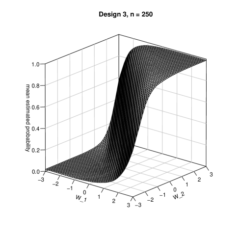
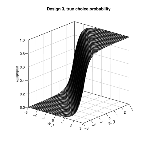
Figure 4: Average (over 500 simulations) estimated (first 3 figures) and true (bottom right) choice probabilities as functions of covariates in Design 3

Figure 2 in the present paper and Figure 4 in Khan, (2013) indicate that both procedures suffer from a substantial bias. Overall, the shape is reproduced better by the sieve procedure in Khan, (2013) which is expected since asymptotically the sieve should be able to consistently estimate the choice probabilities while this is not the case for our approach. Interestingly, the average MSE of our procedure is lower than that of Khan, (2013) for the sample sizes considered in this simulation. This indicates that sometimes completely non-parametric procedures can only develop their full advantage when the sample size is substantial.

In the final part of this simulation study, we analyse the effect of $a,b$ on estimated choice probabilities. To this end, we consider the three covariate values $(-0.5,-0.5),(0,0)$ and $(0.5,0.5)$ along with all combinations of $1-a\in\{0.01,0.15,0.25\},1-b\in\{0.75,0.85,0.99\}$. Results for Design 1 and 4 are reported in Table 2 and Table 3 while the corresponding results for Design 2 and 3 are deferred to Section B in the Appendix. A close look at both tables reveals that for all choices of $1-a,1-b$ considered there is no big impact on estimation of $p_{w}$ for $w=(0,0)^{T}$. Additionally, only the choice of $a$ has an impact on estimating $p_{w}$ for $w=(-0.5,-0.5)^{T}$ (in this case $p_{w}$ is smaller than $0.5$) and only the choice of $b$ impacts the estimation of $p_{w}$ for $w=(0.5,0.5)^{T}$ (in this case $p_{w}$ is greater than $0.5$). This is in line with the theory.

	n = 250	n = 500	n = 1000
Design 1	0.0097 (0.0062)	0.0057 (0.0065)	0.0032 (0.0031)
Design 2	0.0103 (0.0070)	0.0061 (0.0077)	0.0036 (0.0041)
Design 3	0.0082 (0.0081)	0.0050 (0.0085)	0.0028 (0.0057)
Design 4	0.0511 (0.0692)	0.0435 (0.0617)	0.0391 (0.0600)

Table 1: Average MSE for estimating choice probabilities. Average is taken over an equispaced $50$ by $50$ grid over $[-3,3]^{2}$. Values in brackets correspond to the average MSE of the sieve estimators considered in Khan, (2013) and are taken from that reference.

		1-a  1-b	1-a  1-b	1-a  1-b	1-a  1-b	1-a  1-b	1-a  1-b	1-a  1-b	1-a  1-b	1-a  1-b
		0.01 0.99	0.15 0.99	0.25 0.99	0.01 0.85	0.15 0.85	0.25 0.85	0.01 0.75	0.15 0.75	0.25 0.75
$p_{w}$		n = 250
0.14	RMSE	9.03	7.83	12.13	8.99	7.8	12.12	8.95	7.77	12.12
	bias	2.12	5.3	11.85	2.07	5.28	11.85	2.02	5.26	11.84
0.5	RMSE	10.06	10.03	9.89	9.99	9.95	9.79	9.73	9.67	9.48
	bias	0.33	0.49	0.68	0.15	0.31	0.52	-0.08	0.07	0.28
0.86	RMSE	6.47	6.43	6.39	6.16	6.13	6.1	11.35	11.34	11.34
	bias	-2.91	-2.85	-2.8	-4.49	-4.47	-4.46	-11.28	-11.28	-11.27
	n = 500
0.14	RMSE	7.11	6.08	11.39	7.07	6.06	11.39	7.04	6.03	11.39
	bias	1.69	4.24	11.32	1.64	4.23	11.32	1.6	4.21	11.32
0.5	RMSE	7.6	7.58	7.52	7.57	7.54	7.47	7.49	7.45	7.36
	bias	0.21	0.37	0.53	0.04	0.21	0.38	-0.12	0.03	0.2
0.86	RMSE	4.82	4.78	4.75	4.72	4.7	4.69	11.02	11.02	11.02
	bias	-2.46	-2.41	-2.36	-3.63	-3.62	-3.61	-11.01	-11.01	-11.01
	n = 1000
0.14	RMSE	5.37	5.07	11.07	5.34	5.05	11.07	5.3	5.03	11.07
	bias	2.23	3.78	11.06	2.18	3.76	11.06	2.14	3.75	11.06
0.5	RMSE	5.09	5.09	5.09	5.07	5.05	5.04	5.05	5.02	5
	bias	0.38	0.55	0.7	0.22	0.38	0.54	0.07	0.22	0.38
0.86	RMSE	3.63	3.59	3.56	3.65	3.64	3.63	10.99	10.99	10.99
	bias	-1.93	-1.88	-1.83	-2.88	-2.87	-2.86	-10.99	-10.99	-10.99

Table 2: Estimation quality of conditional choice probabilities for different values of $a,b$. Root mean squared error (RMSE) and bias are multiplied by $100$. Data are generated from Design 1.

		1-a  1-b	1-a  1-b	1-a  1-b	1-a  1-b	1-a  1-b	1-a  1-b	1-a  1-b	1-a  1-b	1-a  1-b
		0.01 0.99	0.15 0.99	0.25 0.99	0.01 0.85	0.15 0.85	0.25 0.85	0.01 0.75	0.15 0.75	0.25 0.75
$p_{w}$		n = 250
0.14	RMSE	6.99	6.72	11.48	6.9	6.64	11.44	6.85	6.59	11.43
	bias	3.32	4.96	11.38	3.24	4.91	11.35	3.18	4.89	11.34
0.5	RMSE	11.87	11.8	11.56	11.75	11.67	11.4	11.57	11.46	11.17
	bias	-0.06	0.11	0.38	-0.25	-0.08	0.2	-0.47	-0.31	-0.03
0.86	RMSE	11.92	11.84	11.77	12.13	12.08	12.03	13.35	13.33	13.32
	bias	-10.89	-10.81	-10.73	-11.22	-11.17	-11.12	-13.06	-13.05	-13.03
		n = 500
0.14	RMSE	5.46	5.55	11.08	5.41	5.53	11.08	5.37	5.51	11.07
	bias	3.61	4.39	11.06	3.55	4.37	11.06	3.5	4.35	11.06
0.5	RMSE	9.49	9.46	9.27	9.46	9.41	9.2	9.42	9.36	9.13
	bias	0.05	0.21	0.42	-0.12	0.05	0.26	-0.27	-0.12	0.1
0.86	RMSE	11.92	11.84	11.77	12.15	12.1	12.05	13.08	13.07	13.06
	bias	-11.31	-11.22	-11.15	-11.57	-11.52	-11.47	-12.89	-12.87	-12.86
		n = 1000
0.14	RMSE	5.02	5.22	10.99	4.97	5.2	10.99	4.92	5.18	10.99
	bias	4.03	4.45	10.99	3.97	4.44	10.99	3.92	4.42	10.99
0.5	RMSE	6.36	6.35	6.33	6.34	6.31	6.29	6.33	6.28	6.24
	bias	0.05	0.21	0.36	-0.12	0.05	0.21	-0.27	-0.11	0.05
0.86	RMSE	11.96	11.88	11.8	12.19	12.14	12.09	12.94	12.93	12.92
	bias	-11.57	-11.49	-11.41	-11.82	-11.77	-11.72	-12.82	-12.81	-12.8

Table 3: Estimation quality of conditional choice probabilities for different values of $a,b$. Root mean squared error (RMSE) and bias are multiplied by $100$. Data are generated from Design 4.

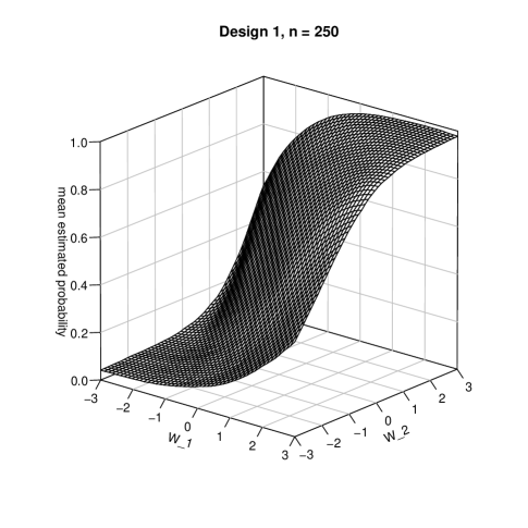
Figure 1: Average (over 500 simulations) estimated (first 3 figures) and true (bottom right) choice probabilities as functions of covariates in Design 1

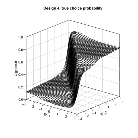
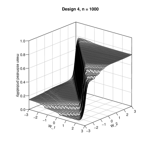
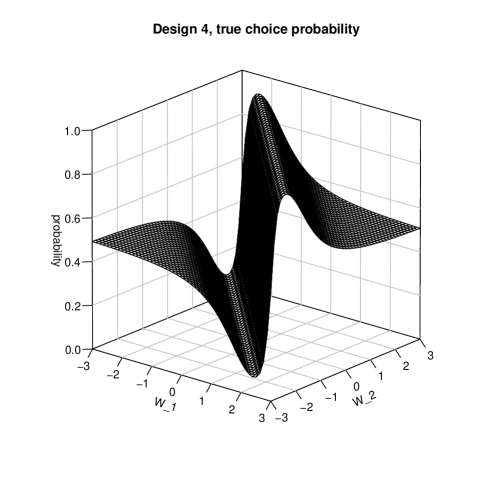
Figure 2: Average (over 500 simulations) estimated (first 3 figures) and true (bottom right) choice probabilities as functions of covariates in Design 4

5 Appendix: Proofs

5.1 Proofs for Section 2

We begin with some useful algebraic identities. First, we prove that under assumptions (A), (D1)-(D5), (M) and (Q)

$$\frac{\partial}{\partial u}\Big{(}F_{Y^{*}|X,Z}(0|x,s_{0}(-x^{T}\bar{b}_{\tau}+u))\Big{)}\Big{|}_{u=0}=-|\beta_{\tau,1}|f_{Y^{*}|X,Z}(0|x,-x^{T}s_{0}\bar{b}_{\tau}).$$ (5.1)

To this end, note that $y(u):=F_{Y^{*}|X,Z}(0|x,s_{0}(-x^{T}\bar{b}_{\tau}+u))$ satisfies the equation (for $u$ sufficiently small)

$$q_{y(u)}((s_{0}(-x^{T}\bar{b}_{\tau}+u),x^{T})^{T})=s_{0}(-x^{T}\bar{b}_{\tau}+u)\beta_{y(u),1}+x^{T}b_{y(u)}=us_{0}\beta_{y(u),1}+x^{T}b_{y(u)}-s_{0}\beta_{y(u),1}x^{T}\bar{b}_{\tau},$$

this follows from the linearity of the conditional quantile function $q_{\tau}(w)=w^{T}\beta_{\tau}$. Additionally $y(0)=\tau$. Thus by the implicit function theorem $u\mapsto y(u)$ is differentiable and its derivative is given by

$$-\frac{\frac{\partial}{\partial u}\Big{(}us_{0}\beta_{y,1}+x^{T}b_{y}-s_{0}\beta_{y,1}x^{T}\bar{b}_{\tau}\Big{)}\Big{|}_{y=\tau,u=0}}{\frac{\partial}{\partial y}\Big{(}us_{0}\beta_{y,1}+x^{T}b_{y}-s_{0}\beta_{y,1}x^{T}\bar{b}_{\tau}\Big{)}\Big{|}_{y=\tau,u=0}}=-s_{0}\beta_{\tau,1}f_{Y^{*}|X,Z}(0|x,-s_{0}x^{T}\bar{b}_{\tau}).$$

Here, the last step follows since

$$\frac{\partial}{\partial y}\Big{(}us_{0}\beta_{y,1}+x^{T}b_{y}-s_{0}\beta_{y,1}x^{T}\bar{b}_{\tau}\Big{)}\Big{|}_{y=\tau,u=0}=\frac{\partial}{\partial y}\Big{(}-s_{0}x^{T}\bar{b}_{\tau},x^{T}\Big{)}\beta_{y}\Big{|}_{y=\tau}=\frac{1}{f_{Y^{*}|X,Z}(0|x,-s_{0}x^{T}\bar{b}_{\tau})}$$

where we used the identities $(-s_{0}x^{T}\bar{b}_{\tau},x^{T})\beta_{y}=q_{y}((-s_{0}x^{T}\bar{b}_{\tau},x^{T})^{T})$ and $q_{\tau}((-s_{0}x^{T}\bar{b}_{\tau},x^{T})^{T})=0$, this shows (5.1). Equation (5.1) implies that, under assumptions (D1)-(D5) and (Q),

$$\frac{\partial}{\partial u}\Big{(}(\tau-F_{Y^{*}|X,Z}(0|x,s_{0}(-x^{T}\bar{b}_{\tau}+u)))f_{Z|X}(s_{0}(-x^{T}\bar{b}_{\tau}+u)|x)\Big{)}\Big{|}_{u=0}\\ =|\beta_{\tau,1}|f_{Y^{*}|X,Z}(0|x,-s_{0}x^{T}\bar{b}_{\tau})f_{Z|X}(-s_{0}x^{T}\bar{b}_{\tau}|x).$$ (5.2)

Proof of (A), (M) and (S) implies (D1) The proof is based on ideas from Manski, (1985). First, let us prove that under (A) and (S) we have for any fixed $\tau\in T$

$$S_{\tau}((s,b^{T})^{T})-S_{\tau}(\beta_{\tau})<0\quad\forall~{}b\in B,s\in\{-1,1\}:(b,s)\neq(\bar{b}_{\tau},s_{0}).$$ (5.3)

To this end, recall the decomposition $S_{\tau}((s,b^{T})^{T})-S_{\tau}(\beta_{\tau})=D_{1}((s,b^{T})^{T},\tau)+D_{2}((s,b^{T})^{T},\tau)$ where

$$D_{1}((s,b^{T})^{T},\tau) = \mathbb{E}[(Y-(1-\tau))I\{sZ+X^{T}b\geq 0>Zs_{0}+X^{T}\bar{b}_{\tau}\}],$$

$$D_{2}((s,b^{T})^{T},\tau) = -\mathbb{E}[(Y-(1-\tau))I\{sZ+X^{T}b<0\leq Zs_{0}+X^{T}\bar{b}_{\tau}\}].$$

Additionally, under (S) we have $E[Y-(1-\tau)|W=w]>0$ if $w^{T}\beta_{\tau}>0$ and $E[Y-(1-\tau)|W=w]<0$ if $w^{T}\beta_{\tau}<0$. This implies that $D_{1}((s,b^{T})^{T},\tau)\leq 0,D_{2}((s,b^{T})^{T},\tau)\leq 0$. Thus it suffices to prove that for $(s,b)\neq(s_{0},\bar{b}_{\tau})$ we have

$$P\Big{(}sZ+X^{T}b>0>Zs_{0}+X^{T}\bar{b}_{\tau}\Big{)}+P\Big{(}sZ+X^{T}b<0<Zs_{0}+X^{T}\bar{b}_{\tau}\Big{)}>0.$$ (5.4)

To see this, begin by observing that under (S) we have $P(X^{T}b\neq X^{T}\bar{b}_{\tau})>0$ if $b\neq\bar{b}_{\tau}$ [otherwise $P(X^{T}(b-\bar{b}_{\tau})=0)=1$ which contradicts the assumption that $X$ is not concentrated on a proper subspace]. Assume without loss of generality that $P(X^{T}b<X^{T}\bar{b}_{\tau})>0$. The assumptions on $Z$ imply that in this case also $P(sZ+X^{T}b<0<s_{0}Z+X^{T}\bar{b}_{\tau})>0$, this can be proved by considering the cases $s=s_{0},s=-s_{0}$ combined with the disjoint events $\{0\leq X^{T}b<X^{T}\bar{b}_{\tau}\}$, $\{X^{T}b<X^{T}\bar{b}_{\tau}\leq 0\}$, $\{X^{T}b<0<X^{T}\bar{b}_{\tau}\}$. For instance, if $s=s_{0}=1$ and $0\leq x^{T}b<x^{T}\bar{b}_{\tau}$ we have $sz+x^{T}b<0<sz+x^{T}\bar{b}_{\tau}$ for $z\in(-x^{T}\bar{b}_{\tau},-x^{T}b)$, which by construction is an interval of positive length for every fixed $x$ satisfying $0\leq x^{T}b<x^{T}\bar{b}_{\tau}$. Thus $P(0\leq X^{T}b<X^{T}\bar{b}_{\tau})>0$ implies $P\Big{(}Z+X^{T}b<0<Z+X^{T}\bar{b}_{\tau}\Big{)}>0$. All other cases are handled similarly. Summarizing we have established that for $b\neq\bar{b}_{\tau}$ (5.4) holds. It remains to consider the case $b=\bar{b}_{\tau},s\neq s_{0}$. From the conditions on $Z$, this case is obvious. This establishes (5.4), and (5.3) follows.

Next, we shall prove (D1) by contradiction. Assume that (D1) does not hold. In that case there exists $\varepsilon>0$ and sequences $(\tau_{n})_{n\in\mathbb{N}}$ in $T$, $(b_{n})_{n\in\mathbb{N}}$ in $B$, $(s_{n})_{n\in\mathbb{N}}$ in $\{-1,1\}$ such that $S_{\tau_{n}}((s_{n},b_{n}^{T})^{T})-S_{\tau_{n}}(\beta_{\tau_{n}})\to 0$ and $\|(s_{n},b_{n})-(s_{0},\bar{b}_{\tau_{n}})\|\geq\varepsilon$. By compactness of $T,B$ there exists a subsequence $n_{k}$ and values $b^{*}\in B,\tau^{*}\in T,s^{*}\in\{-1,1\}$ such that $b_{n_{k}}\to b^{*},s_{n_{k}}\to s^{*},\tau_{n_{k}}\to\tau^{*}$ and $\|(s^{*},b^{*})-(s_{0},\bar{b}_{\tau^{*}})\|\geq\varepsilon$. By continuity of $(s,b,\tau)\mapsto D_{1}((s,b^{T})^{T},\tau)+D_{2}((s,b^{T})^{T},\tau)$ [this follows under (S) by majorized convergence and continuity of the distribution of $sZ+X^{T}b$] we have

$$0=\lim_{n\to\infty}S_{\tau_{n}}((s_{n},b_{n}^{T})^{T})-S_{\tau_{n}}(\beta_{\tau_{n}})=S_{\tau^{*}}((s^{*},(b^{*})^{T})^{T})-S_{\tau^{*}}(\beta_{\tau^{*}}).$$

However, since $\|(s^{*},b^{*})-(s_{0},\bar{b}_{\tau^{*}})\|\geq\varepsilon$, this contradicts (5.3). Thus (D1) follows. $\Box$

Proof of Lemma 2.4 By Lemma 2.6.15 and Lemma 2.6.18 in van der Vaart and Wellner, (1996), the classes of functions $\{(y,w)\mapsto yI\{w^{T}\beta\geq 0\}|\beta\in\mathbb{R}^{d+1}\}$ and $\{w\mapsto I\{w^{T}\beta\geq 0\}|\beta\in\mathbb{R}^{d+1}\}$ are VC-subgraph classes of functions. Together with Theorem 2.6.7 and Theorem 2.4.3 in the same reference this implies

$$\sup_{\tau\in[0,1],\beta\in\mathbb{R}^{d+1}}|S_{\tau}(\beta)-\tilde{S}_{n,\tau}(\beta)|=o(1)\quad a.s.$$

To see this, note that by definition

$$\sup_{\tau\in[0,1],\beta\in\mathbb{R}^{d+1}}|S_{\tau}(\beta)-\tilde{S}_{n,\tau}(\beta)|\leq\sup_{\beta\in\mathbb{R}^{d+1}}\Big{|}\frac{1}{n}\sum_{i}(Y_{i}I\{\beta^{T}W_{i}\geq 0\}-\mathbb{E}[Y_{i}I\{\beta^{T}W_{i}\geq 0\}]\Big{|}\\ +\sup_{\beta\in\mathbb{R}^{d+1}}\Big{|}\frac{1}{n}\sum_{i}(I\{\beta^{T}W_{i}\geq 0\}-P(\beta^{T}W_{i}\geq 0)\Big{|}.$$

Next, observe that almost surely, for any $c>0$,

$$|\hat{S}_{n,\tau}(\beta)-\tilde{S}_{n,\tau}(\beta)|\leq\sup_{|v|\geq c}|\mathcal{K}(v/h_{n})-I\{v\geq 0\}|+(1+\sup_{v}|\mathcal{K}(v)|)\frac{1}{n}\sum_{i=1}^{n}I\{|\beta^{T}W_{i}|\leq ch_{n}\}.$$ (5.5)

Moreover,

$$I\{|\beta^{T}W_{i}|\leq ch_{n}\}=I\{\beta^{T}W_{i}\leq ch_{n}\}-I\{\beta^{T}W_{i}>-ch_{n}\},$$

and the classes of functions $\{w\mapsto I\{w^{T}\beta\leq c\}|\beta\in\mathbb{R}^{d+1},c\in\mathbb{R}\}$, $\{w\mapsto I\{w^{T}\beta>c\}|\beta\in\mathbb{R}^{d+1},c\in\mathbb{R}\}$ are VC-subgraph by Lemma 2.6.15 and Lemma 2.6.18 in van der Vaart and Wellner, (1996). In combination with Theorem 2.6.7 and Theorem 2.4.3 from the same reference this implies

$$\sup_{\beta\in\mathbb{R}^{d+1}}\sup_{c\in\mathbb{R}}\Big{|}\frac{1}{n}\sum_{i=1}^{n}I\{|\beta^{T}W_{i}|\leq ch_{n}\}-P(|\beta^{T}W_{i}|\leq ch_{n})\Big{|}\to 0\quad a.s.$$

Setting $c=c_{n}=h_{n}^{-1/2}$ in the bound for $|\hat{S}_{n,\tau}(\beta)-\tilde{S}_{n,\tau}(\beta)|$ we see that the first term in (5.5), which is independent of $\beta$, converges to zero by assumption (K1). Moreover, by assumption (F1) we have for $\beta=(1,b^{T})^{T}$

$$\sup_{b\in\mathbb{R}^{d}}P(|Z_{i}+b^{T}X_{i}|\leq c_{n}h_{n}) = \sup_{b\in\mathbb{R}^{d}}\int F_{Z|X}(-b^{T}x+h_{n}^{1/2}|x)-F_{Z|X}(-b^{T}x-h_{n}^{1/2}|x)dP_{X}(x)$$

$$= o(1)$$

almost surely. A similar result holds for $\beta=(-1,b^{T})^{T}$. Combining all the results so far we thus see that

$$k_{n}:=\sup_{b\in\mathbb{R}^{d},s=\pm 1}\Big{|}\hat{S}_{n,\tau}((s,b^{T})^{T})-S_{\tau}((s,b^{T})^{T})\Big{|}=o(1)\quad a.s.$$

Finally, observe that any $\beta:=(s_{0},b^{T})^{T}\in\{-1,1\}\times B$ fixed

$$\hat{S}_{n,\tau}(\beta)-\hat{S}_{n,\tau}(\bar{\beta}_{\tau})\leq S_{\tau}(\beta)-S_{\tau}(\bar{\beta}_{\tau})+2k_{n}\leq-d(\|\beta-\bar{\beta}_{\tau}\|)+2k_{n}.$$

Since by definition $\hat{S}_{n,\tau}((\hat{s}_{\tau},\hat{b}_{\tau}^{T})^{T})\geq\hat{S}_{n,\tau}((s,b^{T})^{T})$ for all $s\in\{-1,1\},b\in B$, it follows that $k_{n}<d(\varepsilon)/2$ implies $\sup_{\tau\in T}\|(\hat{s}_{\tau},\hat{b}_{\tau})-(s_{0},\bar{b}_{\tau})\|\leq\varepsilon$. This completes the proof. $\Box$

Proof of Theorem 2.5 Define

$$\tilde{S}_{n}(s,b,\tau) := \frac{1}{n}\sum_{i=1}^{n}(Y_{i}-(1-\tau))\mathcal{K}\Big{(}\frac{X_{i}^{T}b+sZ_{i}}{h_{n}}\Big{)}.$$ (5.6)

First, by uniform consistency of $\hat{\beta}_{\tau}$ and given the fact that $s_{0}\in\{-1,1\}$ we see that with probability tending to one $\hat{s}_{\tau}=s_{0}$ for all $\tau\in T$. Thus we see that with probability tending to one $\hat{b}_{\tau}$ will satisfy

$$\hat{b}_{\tau}=\mbox{argmax}_{b\in B}\hat{S}_{n}(s_{0},b,\tau).$$

Moreover, uniform consistency of $\hat{b}_{\tau}$ implies that with probability tending to one it will satisfy $\sup_{\tau\in T}\|\hat{b}_{\tau}-\bar{b}_{\tau}\|\leq\eta$, and continuous differentiability of $b\mapsto\tilde{S}_{n}(s,b,\tau)$ for $b$ with $\|b-\bar{b}_{\tau}\|\leq\eta$ implies that, with probability tending to one,

$$\tilde{T}_{n}(s_{0},\hat{b}_{\tau},\tau)=0\quad\forall\tau\in T.$$

A Taylor expansion now yields that with probability tending to one

$$\tilde{T}_{n}(s_{0},\bar{b}_{\tau},\tau)+\tilde{Q}_{n}(s_{0},b^{*}_{\tau},\tau)(\hat{b}_{\tau}-\bar{b}_{\tau})=0\quad\forall\tau\in T$$ (5.7)

where

$$\tilde{Q}_{n}(s,b,\tau):=\frac{\partial\tilde{T}_{n}(s,b,\tau)}{\partial b}=\frac{1}{nh_{n}^{2}}\sum_{i=1}^{n}(Y_{i}-(1-\tau))X_{i}X_{i}^{T}K^{\prime}\Big{(}\frac{X_{i}^{T}b+sZ}{h_{n}}\Big{)}$$ (5.8)

and $b^{*}_{\tau}=\xi_{n}(\tau)\bar{b}_{\tau}+(1-\xi_{n}(\tau))\hat{b}_{\tau}$ for some $\xi_{n}(\tau)\in[0,1]$. Define

$$Q(s,b,\tau):=\int\frac{\partial}{\partial u}\Big{(}(\tau-F_{Y^{*}|X,Z}(0|x,s(-x^{T}b+u)))f_{Z|X}(s(-x^{T}b+u)|x)\Big{)}\Big{|}_{u=0}xx^{T}dP_{X}(x).$$ (5.9)

Rearranging (5.7) we obtain

$$Q(s_{0},\bar{b}_{\tau},\tau)(\hat{b}_{\tau}-\bar{b}_{\tau})=-\tilde{T}_{n}(s_{0},\bar{b}_{\tau},\tau)-(\tilde{Q}_{n}(s_{0},b^{*}_{\tau},\tau)-Q(s_{0},\bar{b}_{\tau},\tau))(\hat{b}_{\tau}-\bar{b}_{\tau}).$$ (5.10)

Since $\|\hat{b}_{\tau}-\bar{b}_{\tau}\|_{\infty}=o_{P}(1)$ uniformly over $\tau\in T$ and since the same holds for $\tilde{T}_{n}(s_{0},\bar{b}_{\tau},\tau)$ [see Lemma 5.2], there exists a $\gamma_{n}\to 0$ such that

$$\sup_{\tau\in T}\Big{\|}-\tilde{T}_{n}(s_{0},\bar{b}_{\tau},\tau)-(\tilde{Q}_{n}(s_{0},b^{*}_{\tau},\tau)-Q(s_{0},\bar{b}_{\tau},\tau))(\hat{b}_{\tau}-\bar{b}_{\tau})\Big{\|}=o_{P}(\gamma_{n}).$$

By the conditions on $Q(s_{0},\bar{b}_{\tau},\tau)$ this implies $\sup_{\tau}\|\hat{b}_{\tau}-\bar{b}_{\tau}\|=o_{P}(\gamma_{n})$. By Lemma 5.1 this in turn implies [here, for matrix $A=(a_{ij})_{i,j}$ define $\|A\|_{max}:=\max_{i,j}|a_{ij}|$]

$$\sup_{\tau\in T}\Big{\|}\tilde{Q}_{n}(s_{0},b^{*}_{\tau},\tau)-Q(s_{0},\bar{b}_{\tau},\tau)\Big{\|}_{max}=O_{P}((nh_{n}^{3})^{-1/2}\log n)+O(h_{n}+\alpha_{n})+o_{P}(\gamma_{n}).$$

Finally, note that by (5.2) we have $Q(s_{0},\bar{b}_{\tau},\tau)=Q_{0}(\tau)$. Plugging this into (5.10) and repeating this argument [note that every application yields an improvement of the bound until $\gamma_{n}\sim\sup_{\tau}\|\tilde{T}_{n}(s_{0},\bar{b}_{\tau},\tau)\|$] yields the assertion (2.2).
For a proof of assertion (2.3) fix $1\leq j,j^{\prime}\leq d$. Observe that

$$\mbox{Cov}\Big{(}\sqrt{nh_{n}}(\tilde{T}_{n}(s_{0},\bar{b}_{\tau},\tau))_{j},\sqrt{nh_{n}}(\tilde{T}_{n}(s_{0},\bar{b}_{\kappa},\kappa))_{j^{\prime}}\Big{)}$$

$$= \frac{1}{nh_{n}}\sum_{i,i^{\prime}=1}^{n}\mbox{Cov}\Big{(}(Y_{i}-(1-\tau))X_{ij}K\Big{(}\frac{X_{i}^{T}\bar{b}_{\tau}+s_{0}Z_{i}}{h_{n}}\Big{)},(Y_{i^{\prime}}-(1-\kappa))X_{i^{\prime}j^{\prime}}K\Big{(}\frac{X_{i^{\prime}}^{T}\bar{b}_{\kappa}+s_{0}Z_{i^{\prime}}}{h_{n}}\Big{)}\Big{)}$$

$$= \frac{1}{h_{n}}\mbox{Cov}\Big{(}(Y_{1}-(1-\tau))X_{1j}K\Big{(}\frac{X_{1}^{T}\bar{b}_{\tau}+s_{0}Z_{1}}{h_{n}}\Big{)},(Y_{1}-(1-\kappa))X_{1j^{\prime}}K\Big{(}\frac{X_{1}^{T}\bar{b}_{\kappa}+s_{0}Z_{1}}{h_{n}}\Big{)}\Big{)}.$$

Now by the boundedness of the support of $\mathcal{X}$ and the assumptions on $K$

$$\mathbb{E}\Big{|}(Y_{1}-(1-\tau))X_{1j}K\Big{(}\frac{x^{T}\bar{b}_{\tau}+s_{0}z}{h_{n}}\Big{)}\Big{|}\leq C\int_{\mathcal{X}}\int_{\mathbb{R}}\Big{|}K\Big{(}\frac{X_{1}^{T}\bar{b}_{\tau}+s_{0}z}{h_{n}}\Big{)}\Big{|}f_{Z|X}(z|x)dzdP_{X}(x)=O(h_{n}).$$

Thus it follows that for any $\delta>0$

$$\Big{|}\mbox{Cov}\Big{(}\sqrt{nh_{n}}(\tilde{T}_{n}(s_{0},\bar{b}_{\tau},\tau))_{j},\sqrt{nh_{n}}(\tilde{T}_{n}(s_{0},\bar{b}_{\kappa},\kappa))_{j^{\prime}}\Big{)}\Big{|}$$

$$\leq~{} \frac{C}{h_{n}}\int\int\Big{|}K\Big{(}\frac{x^{T}\bar{b}_{\tau}+s_{0}z}{h_{n}}\Big{)}K\Big{(}\frac{x^{T}\bar{b}_{\kappa}+s_{0}z}{h_{n}}\Big{)}\Big{|}f_{Z|X}(z|x)dzdP_{X}(x)+O(h_{n})$$ (5.11)

$$\leq~{} \frac{C}{h_{n}}\int\Big{(}\sup_{|a|\geq\delta h_{n}^{-1}}|K(a)|+\|K\|_{\infty}I\{|w^{T}\beta_{\tau}|<|\beta_{\tau,1}|\delta\}\Big{)}$$

$$\quad\quad\quad\times\Big{(}\sup_{|a|\geq\delta h_{n}^{-1}}|K(a)|+\|K\|_{\infty}I\{|w^{T}\beta_{\kappa}|<|\beta_{\kappa,1}|\delta\}\Big{)}dP_{W}(w)+O(h_{n})$$

The assumptions on $K$ imply that for any $\delta>0$ we have $\sup_{|a|\geq\delta h_{n}^{-1}}|K(a)|=o(h_{n}^{k_{0}})$. Thus it remains to consider the integral

$$\frac{1}{h_{n}}\int_{\mathbb{R}}I\{|W^{T}\beta_{\kappa}|<|\beta_{\kappa,1}|\delta\}I\{|W^{T}\beta_{\tau}|<|\beta_{\tau,1}|\delta\}dP_{W}(w)\leq\frac{1}{h_{n}}P\Big{(}|W^{T}(\beta_{\tau}-\beta_{\kappa})|\leq 2\delta\max(|\beta_{\kappa,1}|,|\beta_{\tau,1}|)\Big{)}$$

By assumption $w^{T}\beta_{\tau}$ is the conditional $\tau$-quantile of $Y^{*}$ given $W=w$. Hence, for any fixed $w\in\mathcal{W}$, $w^{T}\beta_{\tau}=F_{Y^{*}|W}^{-1}(\tau|w)$. Under assumption (D6) we have $|F_{Y^{*}|W}(y_{1}|w)-F_{Y^{*}|W}(y_{2}|w)|\leq|y_{1}-y_{2}|\sup_{y,w}f_{Y^{*}|W}(y|w)=:f_{\infty}|y_{1}-y_{2}|$ for any $w\in\mathcal{W}$. Substituting $y_{1}=F_{Y^{*}|W}^{-1}(\tau|w)=w^{T}\beta_{\tau},y_{2}=F_{Y^{*}|W}^{-1}(\kappa|w)=w^{T}\beta_{\kappa}$ we find that $|w^{T}(\beta_{\tau}-\beta_{\kappa})|\geq f_{\infty}^{-1}|\tau-\kappa|$ for any $w\in\mathcal{W}$. Hence

$$P\Big{(}|W^{T}(\beta_{\tau}-\beta_{\kappa})|\leq 2\delta\max(|\beta_{\kappa,1}|,|\beta_{\tau,1}|)\Big{)}=0$$

provided that $2\max(|\beta_{\kappa,1}|,|\beta_{\tau,1}|)\delta<f_{\infty}^{-1}|\tau-\kappa|/2$. Since $\delta>0$ can be chosen to be arbitrarily small we obtain that

$$\mbox{Cov}\Big{(}\sqrt{nh_{n}}(\tilde{T}_{n}(s_{0},\bar{b}_{\tau},\tau))_{j},\sqrt{nh_{n}}(\tilde{T}_{n}(s_{0},\bar{b}_{\kappa},\kappa))_{j^{\prime}}\Big{)}=o(1)$$

for any $1\leq j,j^{\prime}\leq d$ and $\tau\neq\kappa$. The rest of the proof follows by standard arguments and is omitted. $\Box$

Lemma 5.1

Under assumptions (A), (M), (K1), (K2), (B), (D2), (D3), (D5) we have [$\alpha_{n}$ was defined in assumption (K2)]

$$\sup_{\tau\in T}\sup_{\|b-\bar{b}_{\tau}\|\leq\eta}\Big{\|}\mathbb{E}[\tilde{Q}_{n}(s_{0},b,\tau)]-Q(s_{0},b,\tau)\Big{\|}_{max}=O(h_{n}+\alpha_{n}),$$ (5.12)

$$\sup_{\tau\in T}\sup_{\|b-\bar{b}_{\tau}\|\leq\eta}\Big{\|}\tilde{Q}_{n}(s_{0},b,\tau)-\mathbb{E}[\tilde{Q}_{n}(s_{0},b,\tau)]\Big{\|}_{max}=O_{P}((nh_{n}^{3})^{-1/2}\log n),$$ (5.13)

where $\tilde{Q}_{n}(s,b,\tau)$ was defined in (5.8) and $Q(s_{0},b,\tau)$ in (5.9). Moreover, we have for any $a_{n}\to 0$

$$\sup_{\tau\in T}\sup_{\|b-\bar{b}_{\tau}\|\leq a_{n}}\Big{\|}Q(s_{0},\bar{b}_{\tau},\tau)-Q(s_{0},b,\tau)\Big{\|}_{max}\leq Ca_{n}$$ (5.14)

for $a_{n}$ small enough and some universal constant $C$.

Proof We begin by considering assertion (5.12). Observe that

$$\mathbb{E}[\tilde{Q}_{n}(s_{0},b,\tau)]=\frac{1}{h_{n}^{2}}\int\int(\tau-F_{Y^{*}|X,Z}(0|x,z))f_{Z|X}(z|x)xx^{T}K^{\prime}\Big{(}\frac{x^{T}b+s_{0}z}{h_{n}}\Big{)}dzdP_{X}(x)$$

$$= \frac{1}{h_{n}}\int\int\Big{(}\tau-F_{Y^{*}|X,Z}(0|x,s_{0}(vh_{n}-x^{T}b))\Big{)}f_{Z|X}(s_{0}(vh_{n}-x^{T}b)|x)xx^{T}K^{\prime}(v)dvdP_{X}(x).$$

The assertion now follows from a Taylor expansion, the assumptions on $K$, and standard arguments similar to those given in Horowitz, (2009). For a proof of (5.13) note that for $i,j=1,...,d$ we have

$$\sup_{\tau\in T}\sup_{\|b-\bar{b}_{\tau}\|\leq\eta}\Big{|}\Big{(}\tilde{Q}_{n}(s_{0},b,\tau)-\mathbb{E}[\tilde{Q}_{n}(s_{0},b,\tau)]\Big{)}_{i,j}\Big{|}\leq h_{n}^{-2}n^{-1/2}\sup_{f\in\mathcal{F}_{n}^{i,j}}|\mathbb{G}_{n}(f)|$$

where $\mathcal{F}_{n}^{i,j}$ denotes the $n-$dependent class of functions

$$\mathcal{F}_{n}^{i,j}:=\Big{\{}f_{n,b,\tau}(x,y,z)=K^{\prime}\Big{(}\frac{x^{T}(\bar{b}_{\tau}+b)+s_{0}z}{h_{n}}\Big{)}(y-(1-\tau))x_{i}x_{j}\Big{|}b\in\mathbb{R}^{d},\|b\|\leq\eta,\tau\in T\Big{\}}$$

and

$$\mathbb{G}_{n}(f):=n^{-1/2}\sum_{i=1}^{n}(f(X_{i},Y_{i},Z_{i})-\mathbb{E}[f(X_{i},Y_{i},Z_{i})]).$$

Now uniform Hölder continuity of $K^{\prime}$, uniform Hölder continuity of $\tau\mapsto b_{\tau}$, and uniform boundedness of $x$ implies that for every sufficiently small $\delta>0$ we have for all $|\tau-\tau^{\prime}|\leq\delta,\|b-b^{\prime}\|\leq\delta$ for some $\gamma>0$

$$\|f_{n,b,\tau}-f_{n,b^{\prime},\tau^{\prime}}\|_{\infty}\leq\frac{C}{h_{n}}(|\tau-\tau^{\prime}|^{\gamma}+\|b-b^{\prime}\|^{\gamma})$$

with $C$ denoting some constant independent of $n,\tau,\tau^{\prime},b,b^{\prime}$. This shows that for sufficiently small $\varepsilon$ the $\|\cdot\|_{\infty}$-bracketing number [see van der Vaart and Wellner, (1996), Chapter 2] of the class $\mathcal{F}_{n}^{i,j}$ is bounded by

$$\mathcal{N}_{[~{}]}(\varepsilon,\mathcal{F}_{n}^{i,j},\|\cdot\|_{\infty})\leq\tilde{C}h_{n}^{-(d+1)/\gamma}\varepsilon^{-(d+1)/\gamma}.$$

Next, observe that for any $\tau\in T,\|b\|\leq\eta$

$$\mathbb{E}[f_{n,b,\tau}^{2}(X,Y,Z)] \leq C\int\int_{\mathbb{R}}\Big{|}K^{\prime}\Big{(}\frac{x^{T}(\bar{b}_{\tau}+b)+s_{0}z}{h_{n}}\Big{)}\Big{|}^{2}dzdP_{X}(x)=C\int\int_{\mathbb{R}}|K^{\prime}(zh_{n}^{-1})|^{2}dzdP_{X}(x)$$

$$= h_{n}C\int_{\mathbb{R}}|K^{\prime}(z)|^{2}dz.$$

Combining this with Lemma A.1 yields

$$\sup_{f\in\mathcal{F}_{n}^{i,j}}|\mathbb{G}_{n}(f)|=O_{P}(h_{n}^{1/2}\log n),$$

and thus the proof of (5.13) is complete. Finally, assertion (5.14) follows by the smoothness properties of $F_{Y^{*}|X,Z}$ and $f_{Z|X}$. Thus the proof is complete. $\Box$

Lemma 5.2

Under assumptions (A), (M), (K1)-(K3), (B), (D2), (D4), (D5) we have

$$\sup_{\tau\in T}\Big{\|}\mathbb{E}[\tilde{T}_{n}(s_{0},\bar{b}_{\tau},\tau)]-T_{n}(s_{0},\bar{b}_{\tau},\tau)\Big{\|}=o(h_{n}^{k_{0}}),$$ (5.15)

$$\sup_{\tau\in T}\Big{\|}\tilde{T}_{n}(s_{0},\bar{b}_{\tau},\tau)-\mathbb{E}[\tilde{T}_{n}(s_{0},\bar{b}_{\tau},\tau)]\Big{\|}=O_{P}((nh_{n})^{-1/2}\log n).$$ (5.16)

Proof The proof of (5.16) follows by arguments very similar to those used to establish (5.13) and is therefore omitted. For the proof of (5.15), note that

$$\mathbb{E}[\tilde{T}_{n}(s_{0},\bar{b}_{\tau},\tau)]=\frac{1}{h_{n}}\int\int x(\tau-F_{Y^{*}|X,Z}(0|x,z))K\Big{(}\frac{s_{0}z+x^{T}\bar{b}_{\tau}}{h_{n}}\Big{)}f_{Z|X}(z|x)dzdP_{X}(x)$$

$$= |s_{0}|\int\int x\Big{(}\tau-F_{Y^{*}|X,Z}(0|x,s_{0}(vh_{n}-x^{T}\bar{b}_{\tau}))\Big{)}f_{Z|X}(s_{0}(vh_{n}-x^{T}\bar{b}_{\tau})|x)K(v)dvdP_{X}(x).$$

$$= \int\int_{|vh_{n}|>\eta}x\Big{(}\tau-F_{Y^{*}|X,Z}(0|x,s_{0}(vh_{n}-x^{T}\bar{b}_{\tau}))\Big{)}f_{Z|X}(s_{0}(vh_{n}-x^{T}\bar{b}_{\tau})|x)K(v)dvdP_{X}(x)$$

$$+\int\int_{|vh_{n}|\leq\eta}x\Big{(}\tau-F_{Y^{*}|X,Z}(0|x,s_{0}(vh_{n}-x^{T}\bar{b}_{\tau}))\Big{)}f_{Z|X}(s_{0}(vh_{n}-x^{T}\bar{b}_{\tau})|x)K(v)dvdP_{X}(x).$$

The order of the first integral is $o(h_{n}^{k_{0}})$ by the assumptions on $K$. The assertion now follows by a Taylor expansion of the function

$$u\mapsto\Big{(}\tau-F_{Y^{*}|X,Z}(0|x,s_{0}(u-x^{T}\bar{b}_{\tau}))\Big{)}f_{Z|X}(s_{0}(u-x^{T}\bar{b}_{\tau})|x),$$

which holds for $|u|\leq\eta$ the assumptions on $K$ and standard arguments. $\Box$

5.2 Proofs for Section 3

Proof of Theorem 3.2 We will prove the result by applying Theorem 3.4 with $Q=\mathcal{W}_{0}$, $g_{w}(\tau):=w^{T}\bar{\beta}_{\tau}I\{\tau\in(a_{w},b_{w})\}-MI\{\tau<a_{w}\}+MI\{\tau>b_{w}\}$, $g_{n,w}(\tau):=w^{T}\hat{\beta}_{\tau}I\{\tau\in(a_{w},b_{w})\}-MI\{\tau<a_{w}\}+MI\{\tau>b_{w}\}$ where $M>0$ is a fixed constant. Note that this definition ensures that $\hat{p}_{w}(a_{w},b_{w})=\Psi_{g_{n,w}}(0),p_{w}=\Psi_{g_{w}}(0)$. Since $g_{w}(\tau)=0$ is equivalent $w^{T}\beta_{\tau}=0$, $g_{w}$ has a unique zero in $u_{0,w}=\tau_{w}$. Next, observe that $\tau\mapsto g_{w}(\tau)$ is continuously differentiable on $T^{\delta}$. Its derivative is given by

$$\frac{\partial}{\partial\tau}w^{T}\bar{\beta}_{\tau}=\frac{s_{0}}{\beta_{\tau,1}}\Big{[}\frac{\partial}{\partial\tau}w^{T}\beta_{\tau}\Big{]}+w^{T}\beta_{\tau}\frac{\partial}{\partial\tau}\frac{s_{0}}{\beta_{\tau,1}}=\frac{s_{0}}{\beta_{\tau,1}f_{Y^{*}|W}(q_{\tau}(w)|w)}+w^{T}\beta_{\tau}\frac{\partial}{\partial\tau}\frac{s_{0}}{\beta_{\tau,1}}$$

where we used the fact that

$$\frac{\partial}{\partial\tau}w^{T}\beta_{\tau}=\frac{\partial}{\partial\tau}F_{Y^{*}|W}^{-1}(\tau|w)=\frac{1}{f_{Y^{*}|W}(q_{\tau}(w)|w)}.$$

This shows that the derivative of $\tau\mapsto g_{w}(\tau)$ is uniformly Hölder continuous with exponent and constant uniform in $w\in\mathcal{W}_{0}$. Additionally, the derivative of $\tau\mapsto g_{w}(\tau)$ in the point $\tau_{w}$ is given by $(|\beta_{\tau_{w},1}|f_{Y^{*}|W}(0|w))^{-1}$, and thus is bounded away from zero uniformly over $w\in\mathcal{W}_{0}$. Next, we show that for all $\varepsilon>0$ we have

$$\inf_{w\in\mathcal{W}_{0}}\inf_{|\tau-\tau_{w}|>\varepsilon,\tau\in T^{\delta}}|g_{w}(\tau)-g_{w}(\tau_{w})|>0.$$ (5.17)

This can be proved by contradiction. To this end, observe that for $w\in\mathcal{W}_{0}$ fixed we have $\inf_{|\tau-\tau_{w}|>\varepsilon,\tau\in T^{\delta}}|g_{w}(\tau)-g_{w}(\tau_{w})|>0$ for all $\varepsilon>0$, this follows by compactness of $T^{\delta}$ and since $\tau\mapsto g_{w}(\tau)$ has a unique zero on $T^{\delta}$. Moreover, under the assumptions made one can prove that $w\mapsto\tau_{w}$ and $(w,\tau)\mapsto g_{w}(\tau)$ are continuous. Now the proof by contradiction follows by the same arguments as given in the last paragraph of the proof that (D1) follows from (A) and (S). The details are omitted for the sake of brevity. To apply Theorem 3.4, it remains to establish that (3.5)-(3.7) hold. Here, (3.5) follows from Lemma 5.3 which we prove next while (3.6), (3.7) follow from the definition of $g_{w},g_{n,w}$, Theorem 2.4 and Lemma 5.2. This yields (3.4). The rest of the proofs follows by standard arguments and is omitted. $\hfill\Box$

Lemma 5.3

Under the assumptions of Theorem 3.2 we have for any $r_{n}=o(h_{n})$

$$\sup_{w\in\mathcal{W}_{0}}\sup_{|\tau-\tau_{w}|\leq r_{n}}\|\hat{\beta}_{\tau_{w}}-\hat{\beta}_{\tau}-(\bar{\beta}_{\tau_{w}}-\bar{\beta}_{\tau})\|=O_{P}(n^{-1/2}h_{n}^{-3/2}r_{n}\log n)+o_{P}(h_{n}^{k_{0}})+O_{P}(\kappa_{n})$$

where $\kappa_{n}$ is defined in Theorem 2.5.

Proof From Theorem 2.5 we know that $\hat{s}_{\tau}=s_{0}$ for all $\tau\in T^{\delta}$ with probability tending to one, and thus it suffices to find a bound for $\|\hat{b}_{\tau}-\bar{b}_{\tau}-(\hat{b}_{\tau_{w}}-\bar{b}_{\tau_{w}})\|$. Here we have for any $\tau,\tau_{w}\in T^{\delta}$

$$\hat{b}_{\tau}-\bar{b}_{\tau}-(\hat{b}_{\tau_{w}}-\bar{b}_{\tau_{w}})$$

$$= -Q_{0}(\tau)^{-1}\tilde{T}_{n}(s_{0},\bar{b}_{\tau},\tau)+Q_{0}(\tau_{w})^{-1}\tilde{T}_{n}(s_{0},\bar{b}_{\tau_{w}},{\tau_{w}})-Q_{0}(\tau)^{-1}R_{n}(\tau)+Q_{0}(\tau_{w})^{-1}R_{n}(\tau_{w})$$

$$= Q_{0}(\tau_{w})^{-1}\Big{(}\tilde{T}_{n}(s_{0},\bar{b}_{\tau_{w}},{\tau_{w}})-\tilde{T}_{n}(s_{0},\bar{b}_{\tau},\tau)\Big{)}$$

$$+\Big{(}Q_{0}(\tau_{w})^{-1}-Q_{0}(\tau)^{-1}\Big{)}\tilde{T}_{n}(s_{0},\bar{b}_{\tau},\tau)-Q_{0}(\tau)^{-1}R_{n}(\tau)+Q_{0}(\tau_{w})^{-1}R_{n}(\tau_{w})$$

with $R_{n}$ defined in (2.2). Combining conditions (D3) and (T) with the results from Theorem 2.5 and Lemma 5.2 we see that the term in the last line is of order $O_{P}(r_{n}(nh_{n})^{-1/2}\log n+\kappa_{n})+o_{P}(h_{n}^{k_{0}})$. For the first term, note that

$$\sup_{w\in\mathcal{W}_{0}}\sup_{|\tau-\tau_{w}|\leq r_{n}}\Big{\|}\tilde{T}_{n}(s_{0},\bar{b}_{\tau_{w}},{\tau_{w}})-\tilde{T}_{n}(s_{0},\bar{b}_{\tau},\tau)\Big{\|}\leq D_{1,n}+D_{2,n}$$

where

$$D_{1,n} := \Big{(}\sum_{j=1,...,d}\sup_{\|f-g\|_{2}\leq Ch_{n}^{-1/2}r_{n},f,g\in\mathcal{F}_{n,j}}h_{n}^{-1}n^{-1/2}|\mathbb{G}_{n}(f)-\mathbb{G}_{n}(g)|^{2}\Big{)}^{1/2},$$

$$D_{2,n} := \sup_{w\in\mathcal{W}_{0}}\sup_{|\tau-\tau_{w}|\leq r_{n}}\Big{\|}\mathbb{E}[\tilde{T}_{n}(s_{0},\bar{b}_{\tau_{w}},{\tau_{w}})-\tilde{T}_{n}(s_{0},\bar{b}_{\tau},\tau)]\Big{\|},$$

$$\mathbb{G}_{n}(f) := \frac{1}{n}\sum_{i=1}^{n}(f(Z_{i},X_{i},Y_{i})-\mathbb{E}[f(Z_{i},X_{i},Y_{i})]),$$

and the classes of functions $\mathcal{F}_{n,j}$ are given by

$$\mathcal{F}_{n,j}=\Big{\{}(z,x,y)\mapsto K\Big{(}\frac{x^{T}(\bar{b}_{\tau}+b)+s_{0}z}{h_{n}}\Big{)}x_{j}(y-(1-\tau))\Big{|}b\in\mathbb{R}^{d},\|b\|\leq\eta,\tau\in T^{\delta}\Big{\}}.$$

In order to see that the representation for $D_{1,n}$ is true, note that

$$\tilde{T}_{n}(s_{0},\bar{b}_{\tau_{w}},{\tau_{w}})-\tilde{T}_{n}(s_{0},\bar{b}_{\tau},\tau)$$

$$= \frac{1}{nh_{n}}\sum_{i=1}^{n}\Big{(}K\Big{(}\frac{X_{i}^{T}\bar{b}_{\tau}+s_{0}Z_{i}}{h_{n}}\Big{)}(Y_{i}-(1-\tau))-K\Big{(}\frac{X_{i}^{T}\bar{b}_{\tau_{w}}+s_{0}Z_{i}}{h_{n}}\Big{)}(Y_{i}-(1-\tau_{w}))\Big{)}X_{i}.$$

In particular we have for $|\tau-\tau_{w}|\leq r_{n}$ and $n$ large enough

$$\Big{|}K\Big{(}\frac{X_{i}^{T}\bar{b}_{\tau}+s_{0}Z_{i}}{h_{n}}\Big{)}(Y_{i}-(1-\tau))-K\Big{(}\frac{X_{i}^{T}\bar{b}_{\tau_{w}}+s_{0}Z_{i}}{h_{n}}\Big{)}(Y_{i}-(1-\tau_{w}))\Big{|}$$

$$\leq \sup_{|v|\leq 1}\Big{|}K^{\prime}\Big{(}v+\frac{X_{i}^{T}\bar{b}_{\tau}+s_{0}Z_{i}}{h_{n}}\Big{)}\Big{|}\frac{|X_{i}^{T}\bar{b}_{\tau}-X_{i}^{T}\bar{b}_{\tau_{w}}|}{h_{n}}+\sup_{v}|K(v)||\tau-\tau_{w}|.$$

This shows that for sufficiently small $\varepsilon$ the $\|\cdot\|_{\infty}$-bracketing number [see van der Vaart and Wellner, (1996), Chapter 2] of the class $\mathcal{F}_{n,j}$ is bounded by

$$\mathcal{N}_{[~{}]}(\varepsilon,\mathcal{F}_{n,j},\|\cdot\|_{\infty})\leq Ch_{n}^{-(d+1)/\gamma}\varepsilon^{-(d+1)/\gamma}.$$

Moreover, the above bound implies that for $|\tau-\tau_{w}|\leq r_{n}$ we have for $n$ large enough

$$\sup_{w\in\mathcal{W}_{0}}\sup_{|\tau-\tau_{w}|\leq r_{n}}\Big{\|}K\Big{(}\frac{X_{i}^{T}\bar{b}_{\tau}+s_{0}Z_{i}}{h_{n}}\Big{)}(Y_{i}-(1-\tau))-K\Big{(}\frac{X_{i}^{T}\bar{b}_{\tau_{w}}+s_{0}Z_{i}}{h_{n}}\Big{)}(Y_{i}-(1-\tau_{w}))\Big{\|}_{2,P}\leq Ch_{n}^{-1/2}r_{n}$$

where $\|f\|_{2,P}:=(\mathbb{E}[f^{2}(Z_{i},X_{i},Y_{i})])^{1/2}$. Applying Lemma A.1 to the classes of functions $\{f-g|f,g\in\mathcal{F}_{n,j},\|f-g\|_{2,P}\leq Ch_{n}^{-1/2}r_{n}\}$ thus shows that $D_{1,n}=O_{P}(n^{-1/2}h_{n}^{-3/2}r_{n}\log n).$
Next, consider $D_{2,n}$. By the results in Lemma 5.2 we have

$$|D_{2,n}|\leq h_{n}^{k_{0}}C_{k}\sup_{x\in\mathcal{X}}\sup_{w\in\mathcal{W}_{0}}\sup_{|\tau-\tau_{w}|\leq r_{n}}\Big{|}\frac{\partial^{k}}{\partial u^{k}}\Big{(}\Big{(}(\tau-F_{Y^{*}|X,Z}(0|x,s_{0}(-x^{T}\bar{b}_{\tau}+u)))f_{Z|X}(s_{0}(-x^{T}\bar{b}_{\tau}+u)|x)\\ -(\tau_{w}-F_{Y^{*}|X,Z}(0|x,s_{0}(-x^{T}\bar{b}_{\tau_{w}}+u)))f_{Z|X}(s_{0}(-x^{T}\bar{b}_{\tau_{w}}+u)|x)\Big{)}\Big{|}_{u=0}\Big{|}+o(h_{n}^{k_{0}}).$$

From condition (D4) we see that the left-hand side in the above expression is of order $o(h_{n}^{k_{0}})$. Thus the proof is complete. $\Box$

5.3 Proofs for Section 3.1

Proof of Theorem 3.4 The statement (3.8) is a direct consequence of the condition on the collection of functions $g_{q}$ and assumption (3.6).
The main technical ingredient for the remaining proof is the expansion in Lemma 5.4. By the assumptions on the collection $g_{q}$ and on $\chi$ there exists a constant $C_{\chi}<\infty$ such that

$$\inf_{q}\inf_{|u-u_{0,q}|>C_{\chi}R_{n}}|g_{q}(u)|>2R_{n}.$$

Together with conditions (3.6), (3.7) this implies that for sufficiently large $n$ the signs of $g_{q}$ and $g_{n,q}$ coincide of the set $\{u:\delta>|u-u_{0,q}|>C_{\chi}R_{n}\}$ for all $q\in Q$. Together with (3.8) this implies for sufficiently large $n$ and any $C\geq C_{\chi}$

$$\Psi_{g_{q}}(0)-\Psi_{g_{q,n}}(0)=\int_{u_{0,q}-CR_{n}}^{u_{0,q}+CR_{n}}I\{g_{q}(u)\leq 0\}-I\{g_{n,q}(u)\leq 0\}du.$$

Next observe that $\sup_{q}|g_{n,q}(u_{0,q})|\leq R_{n}$. Let $C_{0}:=\max\{C_{\chi},g_{min}^{-1}\}$. Then for all $q\in Q$ we have $g_{q}^{\prime}(u_{0,q})C_{0}R_{n}\geq R_{n}\geq|g_{n,q}(u_{0,q})|$. Hence Lemma 5.4 implies for any $q\in Q$

$$\Big{|}\int_{u_{0,q}-C_{0}R_{n}}^{u_{0,q}+C_{0}R_{n}}I\{g_{q}(u)\leq 0\}du-\int_{u_{0,q}-C_{0}R_{n}}^{u_{0,q}+C_{0}R_{n}}I\{g_{n,q}(u)\leq 0\}du-\frac{g_{n,q}(u_{0,q})}{g_{q}^{\prime}(u_{0,q})}\Big{|}\leq\frac{2\xi(C_{0}R_{n})+4C_{)}R_{n}\chi(C_{0}R_{n})}{g_{q}^{\prime}(u_{0,q})}.$$

Take a supremum over $q$ first on the right and then on the left to complete the proof. $\Box$

Lemma 5.4

Consider functions $g,h:[0,1]\to\mathbb{R}$ and assume that for some $u_{0}\in(0,1)$ we have $g(u_{0})=0$. Additionally, assume that $g$ is continuously differentiable in a neighborhood $U_{\delta}(u_{0})\subset(0,1)$ and that $g^{\prime}(u_{0})>0$. Define

$$\xi(\varepsilon):=\sup_{|u-u_{0}|\leq\varepsilon}|h(u_{0})-h(u)-(g(u_{0})-g(u))|,\quad\chi(\varepsilon):=\sup_{|u-u_{0}|\leq\varepsilon}|g^{\prime}(u)-g^{\prime}(u_{0})|.$$

Then for any $\varepsilon<\delta$ with $|h(u_{0})|\leq g^{\prime}(u_{0})\varepsilon$

$$\Big{|}\int_{u_{0}-\varepsilon}^{u_{0}+\varepsilon}I\{g(u)\leq 0\}du-\int_{u_{0}-\varepsilon}^{u_{0}+\varepsilon}I\{h(u)\leq 0\}du-\frac{h(u_{0})}{g^{\prime}(u_{0})}\Big{|}\leq\frac{2\xi(\varepsilon)+4\varepsilon\chi(\varepsilon)}{g^{\prime}(u_{0})}.$$

Proof. Rewrite

$$I\{h(u)\leq 0\}=I\{h(u_{0})-(g(u_{0})-g(u))-(h(u_{0})-h(u)-(g(u_{0})-g(u)))\leq 0\}$$

and observe that by the properties of $g$ we have

$$\sup_{|u-u_{0}|\leq\varepsilon}|g(u)-g(u_{0})-g^{\prime}(u_{0})(u-u_{0})|\leq\varepsilon\chi(\varepsilon).$$

Thus the indicators $I\{h(u_{0})+g^{\prime}(u_{0})(u-u_{0})\leq 0,|u-u_{0}|\leq\varepsilon\}$ and $I\{h(u_{0})-(g(u_{0})-g(u))-(h(u_{0})-h(u)-(g(u_{0})-g(u)))\leq 0,|u-u_{0}|\leq\varepsilon\}$ can only take different values on a set with Lebesgue measure at most $2(\xi(\varepsilon)+\varepsilon\chi(\varepsilon))/g^{\prime}(u_{0})$. This implies

$$\Big{|}\int_{u_{0}-\varepsilon}^{u_{0}+\varepsilon}I\{h(u)\leq 0\}du-\int_{u_{0}-\varepsilon}^{u_{0}+\varepsilon}I\{h(u_{0})+g^{\prime}(u_{0})(u-u_{0})\leq 0\}du\Big{|}\leq\frac{2(\xi(\varepsilon)+\varepsilon\chi(\varepsilon))}{g^{\prime}(u_{0})}.$$

Recalling that $g(u_{0})=0$, similar arguments yield the bound

$$\Big{|}\int_{u_{0}-\varepsilon}^{u_{0}+\varepsilon}I\{g(u)\leq 0\}du-\int_{u_{0}-\varepsilon}^{u_{0}+\varepsilon}I\{g^{\prime}(u_{0})(u-u_{0})\leq 0\}du\Big{|}\leq\frac{2\varepsilon\chi(\varepsilon)}{g^{\prime}(u_{0})}.$$

Finally, a simple computation shows that for $|h(u_{0})|\leq g^{\prime}(u_{0})\varepsilon$

$$\int_{u_{0}-\varepsilon}^{u_{0}+\varepsilon}I\{g^{\prime}(u_{0})(u-u_{0})\leq 0\}du-\int_{u_{0}-\varepsilon}^{u_{0}+\varepsilon}I\{h(u_{0})+g^{\prime}(u_{0})(u-u_{0})\leq 0\}du=\frac{h(u_{0})}{g^{\prime}(u_{0})}.$$

Thus the proof is complete. $\Box$

Appendix A Technical details

Lemma A.1

Assume that the classes of measurable functions $\mathcal{F}_{n}$ consist of uniformly bounded functions (by a constant not depending on $n$). If additionally

$$N_{[\,]}(\mathcal{F}_{n},\varepsilon,L^{2}(P))\leq Cn^{a}\varepsilon^{-a}$$

for every $\varepsilon\leq\delta_{n}$ and constants $C,a>0$ not depending on $n$, then we have for any $\delta_{n}\sim n^{-b}$ with $b<1/2$

$$\sqrt{n}\sup_{f\in\mathcal{F}_{n},\|f\|_{P,2}\leq\delta_{n}}\Big{(}\int fdP_{n}-\int fdP\Big{)}=O_{P}^{*}\Big{(}\delta_{n}(|\log\delta_{n}|+\log n)\Big{)}.$$

Here, the ^∗ denotes outer probability if the supremum is not measurable [see Chapter 1 in van der Vaart and Wellner, (1996) for a more detailed discussion].

Proof. Start by observing that the uniform boundedness of elements of $\mathcal{F}_{n}$ by $D$ implies that $F\equiv D$ is a measurable envelope function with $L_{2}$-norm $D$. Note that for $\eta_{n}$ sufficiently small

$$\gamma(\eta_{n}) := \eta_{n}D/\sqrt{1+\log N_{[]}(\eta_{n}D,\mathcal{F}_{n},L_{2}(P))}\geq D\eta_{n}/\sqrt{1+\log C+a\log n-a\log(D\eta_{n})}$$

$$\geq D\tilde{C}\eta_{n}/\sqrt{|\log\eta_{n}|+\log n}$$

for some finite constant $\tilde{C}$ depending only on $a,C,D$. Thus the bound in Theorem 2.14.2 in van der Vaart and Wellner, (1996) yields for $\delta_{n}$ sufficiently small [with $\mathbb{E}^{*}$ denoting outer expectation]

$$\mathbb{E}^{*}\Big{[}\sup_{f\in\mathcal{F}_{n}}\Big{|}\int fd\alpha_{n}\Big{|}\Big{]} \leq DJ_{[~{}]}(\delta_{n},\mathcal{F}_{n},L_{2}(P))+\sqrt{n}\int F(u)I\{F(u)>\sqrt{n}\gamma(\delta_{n})\}P(du)$$

$$\leq DC_{1}\int_{0}^{\delta_{n}}|\log\varepsilon|+\log nd\varepsilon+D\sqrt{n}I\Big{\{}D>\frac{D\tilde{C}\sqrt{n}\delta_{n}}{|\log\delta_{n}|+\log n}\Big{\}}$$

$$\leq DC_{2}\delta_{n}(|\log\delta_{n}|+\log n)+D\sqrt{n}I\Big{\{}1>\frac{\tilde{C}\sqrt{n}\delta_{n}}{|\log\delta_{n}|+\log n}\Big{\}}$$

where $\alpha_{n}:=\sqrt{n}(P_{n}-P)$, $P_{n}$ denotes the empirical measure, and $C_{1},C_{2}$ are some finite constants. Here, the second inequality follows by a straightforward calculation and the first inequality is due to the fact that for $\delta_{n}$ sufficiently small by definition

$$J_{[]}(\delta_{n},\mathcal{F}_{n},L_{2}(P))=\int_{0}^{\delta_{n}}\sqrt{1+\log N_{[]}(\varepsilon D,\mathcal{F}_{n},L_{2}(P))}d\varepsilon\leq C_{1}\int_{0}^{\delta_{n}}|\log\varepsilon|+\log nd\varepsilon.$$

Now under the assumption on $\delta_{n}$, the indicator $I\{|\log\delta_{n}|+\log n>\tilde{C}\sqrt{n}\delta_{n}\}$ will be zero for $n$ large enough and thus the proof is complete. $\Box$

Appendix B Additional simulation results

This section contains additional tables and figures for Design 2 and Design 3 in Section 4.

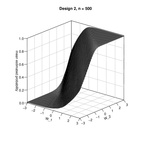
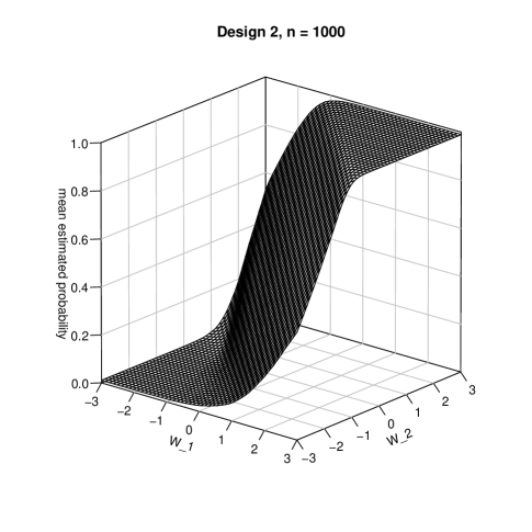
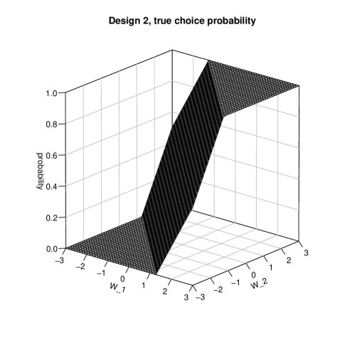
Figure 3: Average (over 500 simulations) estimated (first 3 figures) and true (bottom right) choice probabilities as functions of covariates in Design 2

		1-a  1-b	1-a  1-b	1-a  1-b	1-a  1-b	1-a  1-b	1-a  1-b	1-a  1-b	1-a  1-b	1-a  1-b
		0.01 0.99	0.15 0.99	0.25 0.99	0.01 0.85	0.15 0.85	0.25 0.85	0.01 0.75	0.15 0.75	0.25 0.75
$p_{w}$		n = 250
0.21	RMSE	9.95	8.2	8.12	9.91	8.15	8.09	9.87	8.11	8.06
	bias	0.7	2.44	6.51	0.63	2.4	6.5	0.57	2.36	6.48
0.5	RMSE	9.26	9.23	9.08	9.23	9.19	9.02	9.12	9.06	8.88
	bias	-0.05	0.11	0.3	-0.21	-0.05	0.15	-0.39	-0.24	-0.04
0.79	RMSE	6.08	6.05	6.01	5.79	5.76	5.72	6.04	6.02	6.01
	bias	-1.4	-1.33	-1.27	-1.88	-1.85	-1.81	-5.34	-5.33	-5.33
		n = 500
0.21	RMSE	7.84	6.58	6.59	7.8	6.54	6.57	7.77	6.5	6.55
	bias	0.82	1.93	5.76	0.75	1.89	5.75	0.68	1.86	5.74
0.5	RMSE	6.83	6.81	6.8	6.8	6.77	6.75	6.76	6.71	6.67
	bias	0.12	0.28	0.43	-0.05	0.12	0.28	-0.21	-0.05	0.11
0.79	RMSE	4.75	4.71	4.68	4.69	4.66	4.62	5.21	5.2	5.19
	bias	-1.5	-1.43	-1.36	-1.83	-1.8	-1.76	-4.82	-4.82	-4.81
		n = 1000
0.21	RMSE	5.67	5.2	5.53	5.64	5.17	5.51	5.61	5.14	5.5
	bias	1.18	1.73	5.04	1.11	1.69	5.04	1.04	1.66	5.03
0.5	RMSE	4.7	4.7	4.7	4.68	4.66	4.66	4.66	4.63	4.61
	bias	0.34	0.5	0.65	0.17	0.33	0.49	0.02	0.17	0.33
0.79	RMSE	3.47	3.44	3.41	3.52	3.49	3.47	4.46	4.45	4.45
	bias	-1.15	-1.08	-1.02	-1.43	-1.39	-1.36	-4.28	-4.28	-4.28

Table 4: Estimation quality of conditional choice probabilities for different values of $a,b$. Root mean squared error (RMSE) and bias are multiplied by $100$. Data are generated from Design 2.

		1-a  1-b	1-a  1-b	1-a  1-b	1-a  1-b	1-a  1-b	1-a  1-b	1-a  1-b	1-a  1-b	1-a  1-b
		0.01 0.99	0.15 0.99	0.25 0.99	0.01 0.85	0.15 0.85	0.25 0.85	0.01 0.75	0.15 0.75	0.25 0.75
$p_{w}$		n = 250
0.09	RMSE	7.53	8.13	16.05	7.5	8.12	16.05	7.47	8.1	16.05
	bias	1.49	7.46	16.03	1.46	7.46	16.03	1.43	7.45	16.03
0.5	RMSE	11.04	11.02	10.83	10.99	10.96	10.75	10.6	10.54	10.31
	bias	0.96	1.12	1.34	0.8	0.96	1.18	0.51	0.66	0.88
0.91	RMSE	5.13	5.1	5.07	6.78	6.77	6.77	15.92	15.92	15.92
	bias	-2.32	-2.28	-2.25	-6.56	-6.56	-6.56	-15.92	-15.92	-15.92
		n = 500
0.09	RMSE	5.7	6.96	15.92	5.68	6.96	15.92	5.65	6.95	15.92
	bias	1.48	6.68	15.92	1.45	6.67	15.92	1.42	6.67	15.92
0.5	RMSE	7.91	7.9	7.85	7.87	7.85	7.79	7.8	7.76	7.68
	bias	0.66	0.82	0.98	0.49	0.65	0.82	0.33	0.48	0.65
0.91	RMSE	3.96	3.93	3.9	6.24	6.24	6.24	15.92	15.92	15.92
	bias	-1.95	-1.92	-1.89	-6.15	-6.15	-6.15	-15.92	-15.92	-15.92
		n = 1000
0.09	RMSE	4.47	6.39	15.92	4.44	6.39	15.92	4.42	6.39	15.92
	bias	1.41	6.26	15.92	1.38	6.26	15.92	1.35	6.26	15.92
0.5	RMSE	5.51	5.51	5.51	5.47	5.46	5.46	5.45	5.42	5.4
	bias	0.54	0.71	0.86	0.38	0.54	0.7	0.23	0.38	0.53
0.91	RMSE	3.01	2.98	2.96	6	6	6	15.92	15.92	15.92
	bias	-1.48	-1.45	-1.42	-5.99	-5.99	-5.99	-15.92	-15.92	-15.92

Table 5: Estimation quality of conditional choice probabilities for different values of $a,b$. Root mean squared error (RMSE) and bias are multiplied by $100$. Data are generated from Design 3.

References

- Chaudhuri, (1991) Chaudhuri, P. (1991). Nonparametric estimates of regression quantiles and their local bahadur representation. The Annals of Statistics, 19(2):760–777.
- Chernozhukov et al., (2010) Chernozhukov, V., Fernández-Val, I., and Galichon, A. (2010). Quantile and probability curves without crossing. Econometrica, 78(3):1093–1125.
- Coppejans, (2001) Coppejans, M. (2001). Estimation of the binary response model using a mixture of distributions estimator (mod). Journal of Econometrics, 102(2):231–269.
- Cosslett, (1983) Cosslett, S. (1983). Distribution-free maximum likelihood estimator of the binary choice model. Econometrica, pages 765–782.
- Dette et al., (2006) Dette, H., Neumeyer, N., and Pilz, K. (2006). A simple nonparametric estimator of a strictly monotone regression function. Bernoulli, 12(3):469–490.
- Dette and Volgushev, (2008) Dette, H. and Volgushev, S. (2008). Non-crossing non-parametric estimates of quantile curves. Journal of the Royal Statistical Society: Series B (Statistical Methodology), 70(3):609–627.
- Florios and Skouras, (2008) Florios, K. and Skouras, S. (2008). Exact computation of max weighted score estimators. Journal of Econometrics, 146(1):86–91.
- Friedman et al., (2001) Friedman, J., Hastie, T., and Tibshirani, R. (2001). The elements of statistical learning, volume 1. Springer series in Statistics Springer, Berlin.
- Goffe et al., (1994) Goffe, W. L., Ferrier, G. D., and Rogers, J. (1994). Global optimization of statistical functions with simulated annealing. Journal of Econometrics, 60(1):65–99.
- Hardy et al., (1988) Hardy, G., Littlewood, J., and Polya, G. (1988). Inequalities. Cambridge University Press.
- Horowitz, (1992) Horowitz, J. (1992). A smoothed maximum score estimator for the binary response model. Econometrica, pages 505–531.
- Horowitz, (2009) Horowitz, J. L. (2009). Semiparametric and nonparametric methods in econometrics. Springer Series in Statistics. Springer, New York.
- Ichimura, (1993) Ichimura, H. (1993). Semiparametric least squares (SLS) and weighted SLS estimation of single-index models. Journal of Econometrics, 58(1):71–120.
- Khan, (2013) Khan, S. (2013). Distribution free estimation of heteroskedastic binary response models using probit/logit criterion functions. Journal of Econometrics, 172(1):168 – 182.
- Kim and Pollard, (1990) Kim, J. and Pollard, D. (1990). Cube root asymptotics. The Annals of Statistics, pages 191–219.
- Klein and Spady, (1993) Klein, R. and Spady, R. (1993). An efficient semiparametric estimator for binary response models. Econometrica, pages 387–421.
- Koenker and Bassett, (1978) Koenker, R. and Bassett, G. (1978). Regression quantiles. Econometrica, pages 33–50.
- Kordas, (2006) Kordas, G. (2006). Smoothed binary regression quantiles. Journal of Applied Econometrics, 21(3):387–407.
- Manski, (1975) Manski, C. (1975). Maximum score estimation of the stochastic utility model of choice. Journal of Econometrics, 3(3):205–228.
- Manski, (1985) Manski, C. (1985). Semiparametric analysis of discrete response: Asymptotic properties of the maximum score estimator. Journal of Econometrics, 27(3):313–333.
- Manski, (1988) Manski, C. (1988). Identification of binary response models. Journal of the American Statistical Association, 83(403):729–738.
- Neumeyer, (2007) Neumeyer, N. (2007). A note on uniform consistency of monotone function estimators. Statistics & Probability Letters, 77(7):693–703.
- Portnoy, (1998) Portnoy, S. (1998). Convergence rates for maximal score estimators in binary response regressions. Asymptotic Methods in Probability and Statistics, Editor: B. Szyszkowicz,Elsevier, Amsterdam, pages 775–783.
- Powell et al., (1989) Powell, J., Stock, J., and Stoker, T. (1989). Semiparametric estimation of index coefficients. Econometrica, pages 1403–1430.
- van der Vaart and Wellner, (1996) van der Vaart, A. W. and Wellner, J. A. (1996). Weak Convergence and Empirical Processes. Springer Series in Statistics. Springer, New York.
- Volgushev et al., (2013) Volgushev, S., Birke, M., Dette, H., and Neumeyer, N. (2013). Significance testing in quantile regression. Electronic Journal of Statistics, 7:105–145.