Stochastic bias of colour-selected BAO tracers by joint clustering-weak lensing analysis

Abstract

The baryon acoustic oscillation (BAO) feature in the two-point correlation function of galaxies supplies a standard ruler to probe the expansion history of the Universe. We study here several galaxy selection schemes, aiming at building an emission-line galaxy (ELG) sample in the redshift range $0.6<z<1.7$, that would be suitable for future BAO studies, providing a highly biased galaxy sample. We analyse the angular galaxy clustering of galaxy selections at the redshifts 0.5, 0.7, 0.8, 1 and 1.2 and we combine this analysis with a halo occupation distribution (HOD) model to derive the properties of the haloes these galaxies inhabit, in particular the galaxy bias on large scales. We also perform a weak lensing analysis (aperture statistics) to extract the galaxy bias and the cross-correlation coefficient and compare to the HOD prediction.

We apply this analysis on a data set composed of the photometry of the deep co-addition on Sloan Digital Sky Survey (SDSS) Stripe 82 (225 deg²), of Canda-France-Hawai Telescope/Stripe 82 deep i-band weak lensing survey and of the Wide-Field Infrared Survey Explorer infrared photometric band W1.

The analysis on the SDSS-III/constant mass galaxies selection at $z=0.5$ is in agreement with previous studies on the tracer, moreover we measure its cross-correlation coefficient $r=1.16\pm 0.35$. For the higher redshift bins, we confirm the trends that the brightest galaxy populations selected are strongly biased ($b>1.5$), but we are limited by current data sets depth to derive precise values of the galaxy bias. A survey using such tracers of the mass field will guarantee a high significance detection of the BAO.

Accepted 2013 May 3 by MNRAS.

1 Introduction

Working within the standard cosmological framework described by the Friedmann model, recent analyses of cosmic microwave background (CMB) and Type Ia supernovae (SNIa) data confirm the picture of our Universe as almost spatially flat, with an energy content known at the per cent level and dominated by dark components, and undergoing a phase of accelerated expansion since the last 7 Gyr (e.g. Komatsu et al. 2011; Suzuki et al. 2012). A confirmation of these results is provided by the use of the baryonic acoustic oscillations (BAO) signature in the clustering of galaxies (Frieman et al., 2008), which offers a standard ruler for the measurement of the angular distance–redshift relation. Current measurements of BAO have precision larger than 2 per cent, due to statistical errors. Beutler et al. (2011) provides the latest measurement at $z=0.106$ on the 6dF Galaxy Survey (Jones et al., 2009) with a precision of 4.5 per cent. Blake et al. (2011) and Anderson et al. (2012) made the latest measurements at $z\simeq 0.6$ using, the WiggleZ Dark Energy Survey (Drinkwater et al., 2010) and the Sloan Digital Sky Survey III Baryonic Oscillation Spectroscopic Survey (SDSS-III/BOSS hereafter Eisenstein et al. 2011; Dawson et al. 2013), respectively. At larger redshift $z=2.3$, using the BAO from the Ly$\alpha$ forest of quasars, $H(z=2.3)$ was measured at $\sim 3.5$ per cent (see Pâris et al. 2012; Busca et al. 2013; Lee et al. 2013; Kirkby et al. 2013; Slosar et al. 2013). Future galaxy surveys plan detections of the BAO at the sub-percent level in the redshift range, $0.7\lesssim z\lesssim 2$, to bridge the gap between the forementioned results. It constitutes the next step towards the investigation of the accelerated expansion of the Universe.

The measurement of BAO in the power spectrum of galaxies relies on the assumption that ‘galaxies are tracers of the underlying matter distribution’ (Kaiser, 1984). The validity and the limits of this assumption are not yet completely understood theoretically or observationally. To constrain cosmology with the measurement of the BAO feature in the galaxy clustering, it is necessary to understand the relation between the galaxy distribution and the dark matter field. Currently, to bridge the gap between dark matter haloes and galaxies, there are different methods.

The first approach is to use a model that provides how the galaxies are distributed in haloes (halo occupation distribution model, hereafter HOD; see Dekel & Lahav (1999); Ma & Fry (2000); Seljak (2000); Cooray & Sheth (2002)). The HOD model is fitted on the measure of the galaxy clustering to predict the properties of the haloes that the galaxies inhabit. In particular, HOD predicts the galaxy bias; see White et al. (2011); Zehavi et al. (2011); Parkinson et al. (2012) for the HOD applied to galaxies used in BAO surveys.

The alternative method is based on weak lensing (WL). With recent surveys, it has become possible to combine on small areas (a few deg²) different statistical measures of the galaxy distribution: the galaxy clustering, the cosmic shear, and the galaxy-galaxy lensing. Using Cosmic Evolution Survey (COSMOS) data (Capak et al., 2007; Scoville et al., 2007; Ilbert et al., 2009) Jullo et al. (2012) and Leauthaud et al. (2012) led the way in combining these measures to constrain the galaxy–halo relation and the evolution of the galaxy bias. Improved HOD models are being developed to interpret the combination of both measures (Leauthaud et al., 2011; Cacciato et al., 2012; More et al., 2013; van den Bosch et al., 2013).

The application of such analysis on thousands of square degrees by combining WL with galaxy clustering is however currently limited by the depth and the point spread function (PSF) characterization of the photometry (Huff et al., 2011).

Another possibility to determine the galaxy bias is the direct comparison with large simulations of dark matter using subhalo abundance matching technique (SHAM; Kravtsov et al. 2004; Vale & Ostriker 2004; Conroy et al. 2006; Trujillo-Gomez et al. 2011). Applied to the analysis of WiggleZ and SDSS-III/BOSS observations, this technique shows similar results as the HOD (see Nuza et al. 2013; Parkinson et al. 2012; Prada et al. 2012).

In this paper, we investigate the clustering amplitude of galaxies selected to be the BAO tracers of future large spectroscopic surveys as SDSS-IV/Extended Baryon Oscillation Spectroscopic Survey (eBOSS), BigBOSS, Dark Energy Spectrometer (DESpec), Prime Focus Spectrograph-Subaru Measurement of Image and Redshifts (PFS-SuMiRe), Euclid (Laureijs et al., 2011; Schlegel et al., 2011; Comparat et al., 2013). The clustering amplitude being proportional to $\propto(b\sigma_{8})^{2}$, we consider a constant $\sigma_{8}=0.81$ (value from CMB analysis 7-year Wlikinson Microwave Anisotropy Probe, WMAP7; Komatsu et al. 2011) in order to derive the value of the bias $b$. For this analysis, we combine an HOD approach with a WL analysis. We obtain rather quantitative rough estimates of the galaxy bias, that should not be taken at face value. We make the point for a high clustering amplitude (or a high bias), justifying target selection scheme of future BAO surveys and a more in depth investigation to make forecasts for these surveys accounting for biases at these levels. In fact signal-to-noise ratio (SNR) for BAO studies scales as the density of tracers times the clustering amplitude of these tracers, and hence BAO studies profit from highly clustered tracers.

In section 2 we examine the galaxy bias and the two different methods used to measure it: the HOD model and the WL aperture statistics method. We also discuss the limits of each measurement. In section 3 we describe the data on which our measurement is based. In section 4 we discuss the bias measurement from clustering and WL for each tracer and the associated errors. Finally, in section 5 we discuss the feasibility of future BAO studies using the described tracers.

Throughout this paper we assume a flat $\Lambda$ cold dark matter ($\Lambda$CDM) cosmology characterized by WMAP7 parameters $H_{0}=100\;{\rm km}\;{\rm s}^{-1}\;{\rm Mpc}^{-1}$, with h=0.71, $\Omega_{\mathrm{CDM}}=0.226$, $\Omega_{\mathrm{b}}=0.0455$, $\Omega_{\Lambda}=0.7285$, $\sigma_{8}=0.81$ and $n_{\mathrm{initial}}=0.966$ (Komatsu et al., 2011). Magnitudes are given in the AB system (Oke & Gunn, 1983).

2 Galaxy clustering–weak lensing joint analysis

Galaxy clustering and gravitational lensing probe, respectively, the galaxy overdensity field $\delta_{\mathrm{g}}(\mathbf{r},z)$, which is a discrete random variable function of position $\mathbf{r}$ and redshift $z$, and the matter overdensity field, $\delta_{\mathrm{m}}(\mathbf{r},z)$, which is a discrete random variable related to the latter by some functional form generically called ‘bias’, eventually allowing for stochasticity (Tegmark & Peebles, 1998; Dekel & Lahav, 1999; Tegmark & Bromley, 1999). As random variables, only the $N$-point correlation functions (or functions thereof) are meaningful and can be measured; by combining galaxy clustering and gravitational lensing one can measure the autocorrelation functions $\langle\delta_{\mathrm{g}}^{2}\rangle$ and $\langle\delta_{\mathrm{m}}^{2}\rangle$ and the cross-correlation $\langle\delta_{\mathrm{g}}\delta_{\mathrm{m}}\rangle$ and eventually define the (linear) bias, $b_{\mathrm{g}}$, and stochasticity, $r$, parameters, after Hoekstra et al. (2002)

$$b^{2}_{g}=\frac{\langle\delta_{\mathrm{g}}^{2}\rangle}{\langle\delta_{\mathrm{m}}^{2}\rangle}\;,\;\;r=\frac{\langle\delta_{\mathrm{g}}\delta_{\mathrm{m}}\rangle}{\sqrt{\langle\delta_{\mathrm{g}}^{2}\rangle\langle\delta_{\mathrm{m}}^{2}\rangle}}.$$ (1)

A positive (negative) value for $r$ indicates correlation (anticorrelation) between the galaxy and the matter fields, while $r=1$ ($r=-1$) indicates total correlation (total anticorrelation).

2.1 $b_{\mathrm{g}}$ by clustering, an HOD approach

To derive the galaxy bias, we need the autocorrelation of matter and of galaxies. The galaxy autocorrelation function $\langle\delta_{\mathrm{g}}^{2}\rangle$ is estimated with Landy & Szalay (1993) ‘minimum variance estimator’. Then we use a HOD to interpret the measure of autocorrelation, as it provides an insight into the relation between the galaxies and the haloes they inhabit.

The main ingredients of the model are the following. The halo mass function $n(M,z)$ gives the density of haloes of mass $M$ present at redshift $z$; it is defined as in Sheth & Tormen (1999). The large scale halo bias $b_{\mathrm{h}}(M,z)$ is taken from Sheth et al. (2001) with the parameters and scale dependence described in Tinker et al. (2005). We use the matter autocorrelation from Smith et al. (2003). The parameter of the model is a function that gives the number of galaxies present in a halo of mass $M$, denoted $N(M)$:

$$N(M)=\frac{1}{2}\left[1+\mathrm{erf}\left(\frac{\log M-\log M_{\mathrm{min}}}{\sigma_{\log M}}\right)\right]\left[1+\left(\frac{M-M_{0}}{M_{1}}\right)^{\alpha}\right],$$ (2)

where $\mathrm{erf}(x)=\frac{2}{\pi}\int_{0}^{x}\mathrm{e}^{-t^{2}}\mathrm{d}t$ is the ‘error function’. For a given $N(M)$ the HOD model outputs the corresponding autocorrelation function. A fit on the galaxy autocorrelation function is performed to derive the analytical form of $N(M)$. During the fit, the cosmological parameters are fixed at their fiducial value (WMAP 7). The large-scale galaxy bias of a volume-limited sample of galaxies described by $N(M)$ is obtained with

$$\langle b_{\mathrm{g}}\rangle=\frac{\int n(M,z)b_{\mathrm{h}}(M,z)N(M)\mathrm{d}M}{\int n(M,z)N(M)\mathrm{d}M}.$$ (3)

For more details about the implementation of the HOD we use in this study, see Cooray & Sheth (2002); Tinker et al. (2005); Coupon et al. (2012). We compute angular correlation functions with the software athena and the HOD fits are performed using CosmoPMC; see Kilbinger et al. (2011, 2009, 2010); Coupon et al. (2012).

The main limit of the model is the input autocorrelation of matter. This information is taken from Smith et al. (2003) and has errors of $\sim 8$ per cent at small scales and $<3$ per cent at large scales $k<10h\,\mathrm{Mpc}^{-1}$ in the $\Lambda$CDM paradigm. Also the HOD model is not valid in different cosmological paradigms and can therefore not be used to rule out cosmologies: it can only be used to replace galaxy samples in the galaxy clustering history, which is the aim of this paper.

2.2 $b_{\mathrm{g}}$ and $r$ by weak lensing

Using WL analysis, we derive both $b_{\mathrm{g}}$ and $r$. For this purpose, we need the three auto and cross-correlations mentioned before. The WL measurement is based on the analysis of the distribution of shapes of the galaxies located behind the BAO tracers. Their intrinsic shapes are distorted by the foreground mass around the BAO tracers. The autocorrelation of the ellipticities of the background galaxies contains the information of the matter clustering between the background galaxies and us, $\langle\delta^{2}_{m}\rangle$. The cross-correlation of the ellipticities with the position of the foreground galaxies contains the information of the cross-correlation $\langle\delta_{\mathrm{g}}\delta_{\mathrm{m}}\rangle$. The angular autocorrelation $\langle\delta^{2}_{g}\rangle$ of galaxies is the same as for the HOD.

To be able to compare the auto- and cross-correlation results, the measurements are convolved with Bessel kernels to transform the correlations in aperture correlations. This formalism is described in Schneider et al. (1998) and applied on RCS data in Hoekstra et al. (2002), GaBoDS data in Simon et al. (2007), and on COSMOS in Jullo et al. (2012). We use the same routines as in Jullo et al. (2012) to measure the aperture autocorrelation of galaxies, denoted $\langle\mathcal{N}_{\mathrm{ap}}^{2}(\theta)\rangle$, that of matter, denoted $\langle M_{\mathrm{ap}}^{2}(\theta)\rangle$, and the cross-correlation, denoted $\langle\mathcal{N}_{\mathrm{ap}}(\theta)M_{\mathrm{ap}}(\theta)\rangle$ defined from the power spectrum of the galaxies $P_{n}$, of the matter $P_{\kappa}$, and their cross-power spectrum $P_{n\kappa}$.

$$\langle\mathcal{N}_{\mathrm{ap}}^{2}(\theta)\rangle=2\pi\int_{0}^{\infty}\mathrm{d}l\,lP_{n}(l)\left[\frac{12J_{4}(l\theta)}{\pi(l\theta)^{2}}\right]^{2}$$ (4)

$$\langle M_{\mathrm{ap}}^{2}(\theta)\rangle=2\pi\int_{0}^{\infty}\mathrm{d}l\,lP_{\kappa}(l)\left[\frac{12J_{4}(l\theta)}{\pi(l\theta)^{2}}\right]^{2}$$ (5)

$$\langle\mathcal{N}_{\mathrm{ap}}(\theta)M_{\mathrm{ap}}(\theta)\rangle=2\pi\int_{0}^{\infty}\mathrm{d}l\,lP_{n\kappa}(l)\left[\frac{12J_{4}(l\theta)}{\pi(l\theta)^{2}}\right]^{2}$$ (6)

where $J_{4}$ is the Bessel function of order 4, see Schneider et al. (1998); Simon et al. (2007).
The first output is the galaxy bias in an aperture of an angular radius $\theta$; see equation (7). The second output is the cross-correlation coefficient $r$, that measures the randomness; see equation (8)

$$b(\theta)=f_{1}(\theta,\Omega_{\mathrm{m}},\Omega_{\Lambda})\sqrt{\frac{\langle\mathcal{N}_{\mathrm{ap}}^{2}(\theta)\rangle}{\langle M_{\mathrm{ap}}^{2}(\theta)\rangle}},$$ (7)

$$r(\theta)=f_{2}(\theta,\Omega_{\mathrm{m}},\Omega_{\Lambda})\frac{\langle\mathcal{N}_{\mathrm{ap}}(\theta)M_{\mathrm{ap}}(\theta)\rangle}{\sqrt{\langle\mathcal{N}_{\mathrm{ap}}^{2}(\theta)\rangle\langle M_{\mathrm{ap}}^{2}(\theta)\rangle}}.$$ (8)

The functions $f_{1}$ and $f_{2}$ are normalizations. They correct for the fact that different cosmological volumes are probed by the different statistics. The functions are computed assuming a Smith et al. (2003) non-linear power spectrum with unbiased foreground galaxies ($b=r=1$), that uses the Eisenstein & Hu (1998) transfer function, constrained by the WMAP7 cosmological parameters (Komatsu et al., 2011).

The WL also uses the Smith et al. (2003) non-linear power spectrum and has therefore the same precision limitations as the HOD. Moreover, an additional constraint is that, to be able to extract the WL signal, the sources must be behind the lenses. Because of this point, we are not able to have a significant measure of the matter galaxy cross-correlation by WL for the faintest galaxy samples (see section 3).

3 Data

In this section, we present the data sets that are used for this analysis. First, we explain the catalogues used to target galaxies tracing BAO, and we detail the selection functions for the BAO tracers. Then we describe the dark matter halo simulation we used. Finally, we describe the catalogues containing the galaxy shape measurements.

3.1 SDSS-Stripe 82 galaxy catalogue

The SDSS (York et al., 2000; Eisenstein et al., 2011), delivered under the Data Release 9 (DR9; Ahn et al. 2012), covers 14 555 deg² in the five photometric bands u, g, r, i, z. It is the largest volume multi-colour extragalactic photometric survey available today. The 3$\sigma$ magnitude depths are: $u=22.0$, $g=22.2$, $r=22.2$, $i=21.3$; see Fukugita et al. (1996) for the description of the filters, Gunn et al. (1998) for the characteristics of the camera, and Gunn et al. (2006) for the description of the 2.5m telescope located at Apache Point Observatory (New Mexico, USA).

The data set used here for the selection of the different BAO tracers is the SDSS deep Stripe 82 co-add (Annis et al., 2011). It covers an area of 225 deg² in one continuous stripe $-1^{\circ}.25<\delta_{\mathrm{J2000}}<1^{\circ}.25$, $-34^{\circ}<\alpha_{\mathrm{J2000}}<46^{\circ}$ with five photometric bands u, g, r, i, z. We also use the infrared counterpart of this area observed by Wide-field Infrared Survey Explorer (WISE) at 3.4$\mu$m (Wright et al., 2010). Table 1 gives an overview of the tracers selected in this analysis, see section 3.2.

Table 1: Samples of BAO tracers used in this analysis, ‘b’ stands for bright and ‘f’ for faint. $\bar{z}$ is the mean redshift of the sample, $\sigma_{z}$ is the dispersion of the redshift distribution, $N$ the total amount of tracers in the sample, $N_{S}$ the density of tracers per deg², ‘$\bot$ scale’ is the transverse scale in $h^{-1}$ Mpc corresponding to 1^∘ at $\bar{z}$.

sample	$\bar{z}$	$\sigma_{z}$	$N$	$N_{S}$	$\bot$ scale
				(deg-2)	($h^{-1}\,$Mpc deg-1)
CMASS	0.53	0.10	22k	98	16.0
LRG-WISE b	0.58	0.12	15k	70	17.8
LRG-WISE f	0.69	0.13	59k	275	18.5
ELG gri b	0.80	0.08	119k	530	19.2
ELG gri f	0.81	0.15	226k	1007	19.3
ELG ugri b	0.95	0.24	156k	693	20.3
ELG ugri f	0.94	0.22	436k	1938	20.2
ELG ugr b	1.28	0.36	77k	341	21.5
ELG ugr f	1.26	0.34	237k	1052	21.5

The photometric redshift distribution of the BAO tracers is obtained using the Canada-France-Hawai Telescope (CFHT)-LS Wide W4 field photometric redshift catalogue T0007. The photometric redshift accuracy is estimated to be $\sigma_{z}<0.08(1+z)$ for $i\leq 24$. The data and cataloguing methods are described in Ilbert et al. (2006) and Coupon et al. (2009), and the T0007 release document. The CFHT-LS W4 field overlaps the Stripe 82 on a few square degrees. Both data sets have similar depths in magnitude. From a position match of the targets selected on the stripe 82, we obtain a subcatalogue of the targets with photometric redshifts, from which we infer the redshift distribution of the selections. The redshift distributions are shown in Fig. 1.

With current data, it is not feasible to obtain a reliable photometric redshift on the complete Stripe 82. Therefore, we cannot construct clean volume-limited samples, as required by the HOD analysis. We can only make magnitude-limited samples. The impact of the galaxies located in the tails of redshift distribution on the angular clustering is discussed in Section 4.1.

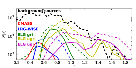
Figure 1: Redshift distributions of the samples. For each sample, solid (dashed) lines refer to the bright (faint) sample. 22 000 CMASS (red), 15 000 (59 000) LRG WISE (blue), 119 000 (226 000) gri ELG (green), 156 000 (436 000) ugri (yellow), 77 000 (237 000) ugr ELG (magenta). The dashed black line represents the redshift distribution of the background sources used in the WL analysis.

3.2 BAO tracer selections

The latest BAO tracers used at $z>0.5$ are SDSS-III Constant Mass galaxies (CMASS) at $z\simeq 0.53$ (Dawson et al., 2013) and WiggleZ emission-line galaxies at $z\simeq 0.6$ (Drinkwater et al., 2010). The next stage BAO experiments plan to use luminous red galaxies (LRG) and emission line galaxies (ELG) at $z>0.7$ (Schlegel et al., 2011). The target selection of ELG tracers is extensively discussed in Comparat et al. (2013).

The selection of the tracers used in this analysis is only based on photometric criteria, depth and colour. We do not use the photometric redshifts for the selection as their quality varies strongly across the stripe. The selection criteria target the most luminous galaxies in incremental redshift intervals to $z=2$; see Fig. 2 which compares all samples in absolute magnitude $M_{i}$ versus redshift or rest-frame $M_{u}-M_{g}$. The cleanest way to select BAO tracers would be to select by stellar mass, but with current data this is not possible.

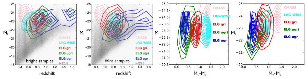
Figure 2: Absolute magnitude $M_{i}$ versus redshift and rest-frame $M_{u}-M_{g}$. All galaxies with $i<23.5$ (grey), CMASS (pink), LRG WISE (light blue), gri ELG (red), ugri ELG (green), ugr ELG (blue). First panel shows the bright selections are quite luminous with $M_{i}\sim-23$. The second panel shows the faint selections are less luminous than the bright selections with $M_{i}\sim-22$. The third panel shows the bright selections span the complete rest-frame colour range from ugr ELG (blue) to the CMASS (pink). The fourth panel shows the faint selections. Their rest frame colours are similar to that of the bright selections, except for the LRG-WISE faint galaxies that are bluer than the bright sample. The ugri ELG overlap with the gri and ugr ELG selections, which is expected as the selection encompasses galaxies from both other selections. This figure was made with the same CFHT W4 matched sample as for the redshift distributions.

3.2.1 CMASS at $z\simeq 0.5$

The CMASS tracer is the SDSS-III/BOSS experiment BAO tracer (Dawson et al., 2013). The current BAO detection using the Data Release 9 (Ahn et al., 2012) (a third of the observation plan) with the CMASS tracers has a $6.7\sigma$ significance (Anderson et al., 2012). Its selection is described in detail in Dawson et al. (2013). The parent catalogue of CMASS selection on Stripe 82 contains 22 034 tracers, i.e. $\sim 98$ deg^-2. We use the complete CMASS selection, not only the galaxies confirmed by spectroscopy, in order to avoid fibre collision issues. The redshift distribution is shown by the red solid line in Fig 1. The mean redshift is 0.53 with a dispersion of 0.1. We use snapshot number 62 of the multidark simulation. The density of the tracer at $\bar{z}$ is $2.64\times 10^{-4}h^{3}$Mpc^-3, which corresponds to a circular velocity cut of $V_{\mathrm{cir}}=384.1$ km s^-1. This value of $V_{cir}$ is consistent with the study done by Nuza et al. (2013). The halo mass distribution peaks at $\log_{10}{M_{200}/M\odot}=13.17_{-0.19}^{+0.34}$. The minimum satellite fraction expected is 5 per cent.

3.2.2 LRG-WISE at $z\simeq 0.65$

This selection is the extension in redshift of the red CMASS selection. We name this sample the ‘luminous red galaxies selected with WISE’ (LRG-WISE) (see Schlegel et al. 2011, Prakash et al., in preparation). On Stripe 82, it selects 15 643 galaxies, i.e. a density of 70 deg^-2 at a mean redshift of 0.58 for the bright sample with $i<20$ and $\sim 59000$ galaxies at a mean redshift of 0.69 for the faint sample with $i<21$, i.e. a density of 262 deg^-2. The selection is as follows:

• we use dereddened r, i, z and 3.4$\mu$m (WISE 1) magnitudes;

• SDSS $z$-band flag must be true, and WISE channel 1 flag must be 0;

• objects with extreme astrometric uncertainties were rejected;

• bright selection: ($i<20\;\mathrm{or}\;z<20$) $and$ $r-i>1$ $and$ $r-W1>2(r-i)-0.5$ $and$ $r>16$ $and$ $r<22.5$;

• faint selection: ($i<21\;\mathrm{or}\;z<21$) $and$ $r-i>1$ $and$ $r-W1>2(r-i)-0.5$ $and$ $r>16$ $and$ $r<22.5$.

The redshift distribution of the bright (faint) samples are shown with a solid (dashed) blue line in Fig. 1. Their densities are $1.57$ and $5.06\times 10^{-4}h^{3}$Mpc^-3, respectively. We use the multidark snapshot 58 for the bright and the faint samples SHAM. The samples correspond to cuts at $V_{\mathrm{cir}}=431.5$ and $323.6$ km s^-1, respectively. The halo mass distributions peak at $\log_{10}{M_{200}/M\odot}=13.28_{-0.17}^{+0.31}$ and $12.92_{-0.2}^{+0.36}$, respectively. They constitute an upper limit for the halo mass these tracer inhabit. The minimum satellite fractions expected are 4 and 7 per cent, respectively.

3.2.3 ELG gri at $z\simeq 0.8$

The gri ELG selection (Comparat et al., 2013) is an intermediate selection between the reddest galaxies selected in SDSS-III and the bluest ones selected by the $ugr$ and $ugri$ schemes (see below), identifies emission-line galaxies with emission lines a small Balmer break. On Stripe 82, it selects $\approx 119\,000$ and $226\,000$ galaxies for the bright and faint samples, which correspond to a projected density of about 530 and 1000 deg^-2 at mean redshift $z\simeq 0.8$ and 0.81, respectively. The bright sample is limited by $19<i<21.5$, and the faint sample by $19<i<22$. The densities are respectively 8.16 and 13.37 $\times 10^{-4}\,h^{3}$Mpc^-3. We use multidark snapshot number 56 to perform the SHAM. The samples match with a circular velocity cut of 292.2 and 250.7 km s^-1. The halo mass distributions peak at $\log_{10}{M_{200}/M\odot}=12.77_{-0.21}^{+0.37}$ and $12.34_{-0.25}^{+0.44}$, respectively. They constitute an upper limit for the halo mass these tracer inhabit. The minimum satellite fractions expected are 8 and 10 per cent, respectively.

3.2.4 ELG ugr at $z\simeq 1.2$

The ugr ELG selection (Comparat et al., 2013) selects the blue tail of the colour distribution aiming for galaxies with strong emission lines at higher redshift ($z\simeq 1.2$). The ugr redshift distribution is flatter and extends to higher redshifts. The bright sample is limited by $20<g<22.5$, and the faint sample by $20<g<23$. For the bright and faint sample it selects, $77\,000$ and $237\,000$ galaxies, corresponding to a density of 341 and 1052 deg^-2, respectively. Their mean redshift are at 1.28 and 1.26. We use multidark snapshot number 48. The bright sample density, $1.45\times 10^{-4}h^{3}$Mpc^-3, corresponds to a cut at 434.5 km s^-1, which gives an upper limit of $\log_{10}{M_{200}/M\odot}\lesssim 13.21_{-0.16}^{+0.29}$. The faint sample density, $5.76\times 10^{-4}h^{3}$Mpc^-3, corresponds to a cut at 315.0 km s^-1, which gives an upper limit of $\log_{10}{M_{200}/M\odot}\lesssim 12.81_{-0.19}^{+0.34}$. The minimum satellite fractions expected are 3 and 7 per cent, respectively.

3.2.5 ELG ugri at $z\simeq 0.95$: building SDSS-IV/eBOSS

The ugri ELG selection is designed to be the BAO tracer sample for SDSS-IV/eBOSS project (eBOSS collaboration, in preparation). It is a mix of the two previous gri and ugr ELG selections. The selection criteria are

• $20<g<22.5$ for the bright; $20<g<23$ for the faint

• $-0.5<u-r<0.7(g-i)+0.1$ and $g-i>-0.5$

The mean redshifts are 0.95 and 0.94. The bright sample contains $156\,000$ galaxies and the faint sample $436\,000$ (i.e. densities of 693 and 1938 deg^-2). We use multidark snapshot number 52 for the SHAM. The densities are respectively 5.44 and 16.45 $\times 10^{-4}h^{3}$Mpc^-3, corresponding to mass upper limits of $\log_{10}{M_{200}/M\odot}\lesssim 12.84_{-0.19}^{+0.35}$ and $\lesssim 12.48_{-0.23}^{+0.4}$. The minimum satellite fractions expected are 7 and 11 per cent, respectively.

3.3 Multidark-Stripe 82 halo catalogue

We use the Multidark dark matter simulation to characterize qualitatively our samples to the first order using SHAM. To perform the match, we use snapshots of the Multidark simulation corresponding to the mean redshift of our tracers. Every snapshot occupies a volume of 1 $h^{-3}$Gpc³ filled with haloes obtained with bound density maximum algorithm with a cut-off at 200 times the critical density ($\log_{10}{M_{\mathrm{200}}/M\odot}$). These data sets are taken from the data base Multidark (Riebe et al., 2011).

In each snapshot, we select the dark matter halo population that corresponds to the number density of galaxies with $\bar{z}-\sigma_{z}<z<\bar{z}+\sigma_{z}$ selected on the Stripe 82. This links each galaxy sample to a halo sample. The density, velocity cuts and characteristic masses and satellite fractions are given for each sample in Table 2.

The SHAM brings two components to this analysis. Under the hypothesis that the galaxy sample is complete in mass. The abundance matched subhalo sample has a mass distribution characterized by the three quartiles of $\log_{10}{M_{\mathrm{200}}/M\odot}$ and a satellite fraction $f_{\mathrm{sat}}$. If the galaxy sample is not complete in mass, the mass distribution of the subhaloes the galaxies live in will be shifted towards lower masses and the satellite fraction will increase. As we cannot demonstrate that the BAO tracers selected are complete in mass and that they are tracing the most massive structure at their redshift, we consider the subhalo mass scales obtained with the SHAM procedure are an upper boundary, and that the satellite fraction is a lower limit to the true values. Moreover, it provides the mass distribution of the subhaloes. Given that we measure clustering over $\sim 200$ deg² and WL on $\sim 150$ deg² and not the full sky, we check the mean halo mass deduced from the maximum likelihood HOD model is between the first and third quartile of the sub-halo mass distribution given by SHAM.

From the qualitative numbers obtained by the SHAM, the LRG-WISE faint sample appears to be located in massive subhaloes of $\sim 10^{13}M\odot$ with a low satellite fraction, similarly to the CMASS tracers. Concerning the ELG, the satellite fraction are higher and the subhalo masses are lower: $\lesssim 10^{12.8}M\odot$ for the bright samples and $\lesssim 10^{12.6}M\odot$ for the faint samples.

Table 2: Abundance matching of the samples of BAO tracers used in this analysis, ‘b’ stands for bright and ‘f’ for faint. The density of tracers is in units of $10^{-4}\,h^{3}$Mpc^-3. $V_{\mathrm{cir}}$ or $V_{\mathrm{max}}$ is the velocity cut applied to the multidark simulation snapshot to match the density $d$. The obtained sample is characterized by the three quartiles of its distributions given in the columns $\log_{10}{M_{\mathrm{200}}/M\odot}$. $f_{\mathrm{sat}}$ is the fraction of satellites in the halo catalogue.

Sample	Density	$V_{\mathrm{cir}}$	$\log_{10}{M_{\mathrm{200}}/M\odot}$	$f_{\mathrm{sat}}$
	$d$	(km s${}^{-1})$	$M_{d}$	(per cent)
CMASS	2.64	384	$13.17_{-0.19}^{+0.34}$	5
LRG-WISE b	1.57	431	$13.28_{-0.17}^{+0.31}$	4
LRG-WISE f	5.06	324	$12.92_{-0.2}^{+0.36}$	7
ELG gri b	8.16	292	$12.77_{-0.21}^{+0.37}$	8
ELG gri f	13.37	251	$12.59_{-0.23}^{+0.41}$	10
ELG ugri b	5.44	317	$12.84_{-0.19}^{+0.35}$	7
ELG ugri f	16.45	238	$12.48_{-0.23}^{+0.4}$	11
ELG ugr b	1.45	435	$13.21_{-0.16}^{+0.29}$	3
ELG ugr f	5.76	315	$12.81_{-0.19}^{+0.34}$	7

3.4 CFHT-Stripe 82 weak-lensing catalogue

The existing comprehensive data sets available on the SDSS Stripe-82 area were complemented with high-quality $i$’-band observations at CFHT. The main purpose of this one-band Megaprime@CFHT (see Boulade et al. 2003) follow-up survey is to enrich already existing multi-colour data with deep optical observations suitable for WL studies. The CFHT Stripe-82 program (CFHT/Stripe 82) is a large collaborative effort between the Canadian/French and Brazilian communities. The observations encompass 169 MegaPrime new pointings resulting in an effective survey area of about 150 deg². This area comprises 169 – 4(due to fringing) = 165 pointings CFHT/Stripe 82 and eight CFHT-LS Wide pointings, i.e. a total of 173 pointings. All the data were obtained under excellent seeing conditions, and the final co-added images show an image quality between 0.4 and 0.8 arcsec with a median of 0.59 arcsec. Each pointing was obtained in four dithered observations with an exposure time of 410s, each resulting in a 5-$\sigma$ limiting magnitude in a 2 arcsec diameter aperture of about 24.

The data processing, which starts with the Elixir preprocessed images obtained from CADC and ends with co-added images and all necessary quantities to perform weak gravitational lensing studies, follows closely the descriptions given in Erben et al. (2012).

We exploit the opportunity that the CFHTLS includes the Hubble Space Telescope HST COSMOS survey field, and verify the calibration of our shear measurement pipeline for ground-based data against an independent analysis of much higher resolution space-based data. We stack the subsets of the CFHTLS DEEP2 imaging to the same depth as the CFHT Stripe 82 survey and analyse it using KSB method (Kaiser et al., 1995). The KSB method is used to measure the shapes of all the selected galaxies. Our implementation of KSB is based on the KSBf90 pipeline (Heymans et al., 2006b). This has been generically tested on simulated images containing a known shear signal as part of the Shear Testing Programme (STEP; Heymans et al. (2006a); Massey et al. (2007)) and the Gravitational lensing Accuracy Testing challenge (GREAT08; Bridle et al. (2010); GREAT10: Kitching et al. (2012)). The systematic errors of this pipeline are well controlled in all cases. This pipeline has also been used on the shear measurement of CFHTLS-Wide W1 fields (Shan et al., 2012). Finally, we match galaxies in the CFHT/Stripe 82 catalogue to those of the HST COSMOS catalogue (Leauthaud et al., 2010) to calibrate the measurements.

Here is the description of the calibration tests we made on the lensing catalogue. The multiplicative calibration component is $(m_{1},m_{2})=(0.13,0.14)$ and the additive component is $(c_{1},c_{2})=(0.0003,0.0015)$. These coefficients are obtained from simulations and connect through the linear relation between the observed galaxy ellipticities and the true ones

$$e^{\mathrm{obs}}=(1+m)[\gamma+e^{\mathrm{true}}]+c$$ (9)

They mainly depend on the algorithm that measures the shapes. If the PSF anisotropy is small, the shear $\gamma$ can be recovered to first-order from the observed ellipticity $e^{\rm obs}$ of each galaxies via

$$\gamma=P_{\gamma}^{-1}\left(e^{\rm obs}-\frac{P^{\rm sm}}{P^{\rm sm*}}e^{*}\right),$$ (10)

where asterisks indicate quantities that should be measured from the PSF model interpolated to the position of the galaxy, $P^{\rm sm}$ is the smear polarisability, and $P_{\gamma}$ is the correction to the shear polarisability that includes the smearing with the isotropic component of the PSF. The ellipticities are constructed from a combination of an object weighted quadrupole moments, and the other quantities involve higher order shape moments. All definitions are taken from Luppino & Kaiser (1997) with the assumption $\kappa\sim 0$, i.e. the reduced shear reads $g=\frac{\gamma}{1-\kappa}\sim\gamma$.

In order to check for significant additive systematics we performed four tests.

1. We test the average shear $\langle\gamma\rangle$ across all 173 pointings of the CFHT/Stripe 82 field. Fig. 3 demonstrates that the average shear is almost consistent with zero as expected, for galaxies of all sizes, magnitudes and SNR. As in Heymans et al. (2012), $\langle g_{2}\rangle$ is clearly dependent on the SNR (red points). We quantify the additive component of the calibration correction with a simple relation $\langle g_{2}\rangle=a+b\,SNR$. We find a best fit reduced $\chi^{2}=0.54$ with $a=-0.002,b=0.000118$. The corrected average shear is almost consistent with zero for galaxies of all sizes, magnitudes and SNR. Furthermore, the average shear of each pointing has also been tested, see Fig. 4. We find that the mean shear $\langle g_{1}\rangle$ of pointing S82p24p is around $-0.0126\pm 0.0017$, which is far from zero compared to other observation pointings. Systematic error residual signal may exist in this pointing. We remove the related galaxies in the final catalogue.

   

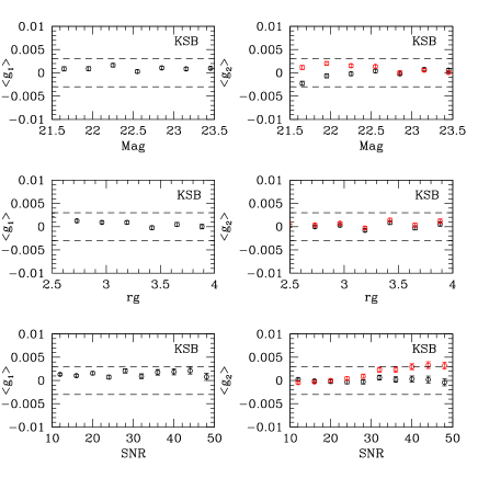
   Figure 3: Average shear measurements $\langle g_{1}\rangle$ (left) and $\langle g_{2}\rangle$ (right) of KSB from galaxies in $i^{\prime}$-band observations of the entire CFHT/Stripe 82 field. In the absence of additive systematics, these should be consistent with zero. In practice, they always remain within the dashed lines that indicate an order of magnitude lower than the $1$–$10$ per cent shear signal around clusters. Top, middle and bottom panels show trends as a function of galaxy magnitude, size and SNR. The black points denote the average shear from all the galaxies in the two shear catalogues. The red points denote $\langle g_{2}\rangle$ before the correction described in (i).

   

   Figure 4: Average shear $\langle g_{1}\rangle$ of $173$ pointings, in which S82p24p field is biased from zero.

2. Star–galaxy cross-correlation (residual systematics due to imperfect PSF). For the total 173 pointings, we find our PSF correction is well within requirements for our analysis. Fig. 5 shows the correlation $\xi_{\mathrm{sys}}$ between the corrected shapes of galaxies and the uncorrected shapes of the stars. We normalize the star-galaxy ellipticity correlation by the uncorrected star-galaxy ellipticity correlation to assess its impact on shear measurements (Bacon et al., 2003); see Fig. 6. Though, we find $\xi_{\mathrm{sys}}$ is obviously higher than $\xi_{+}$ in one pointing S82p35p at scale $\theta>3\rm arcmin$, which reveals the presence of a systematic error residual signal in this pointing. We remove the related galaxies in the final catalogue (only the field with $\delta_{\xi}<0$ is excluded).

   

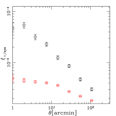
   Figure 5: The cross-correlation between shear measurements and stellar ellipticities as a function of the separation between galaxies and stars, averaged throughout the CFHTLS Stripe 82 field. The black and red points are shear correlation function and star-galaxy cross-correlation, respectively. If all residual influence of the observational PSF has been successfully removed from the galaxy shape measurements, the red points should be consistent with zero.

   

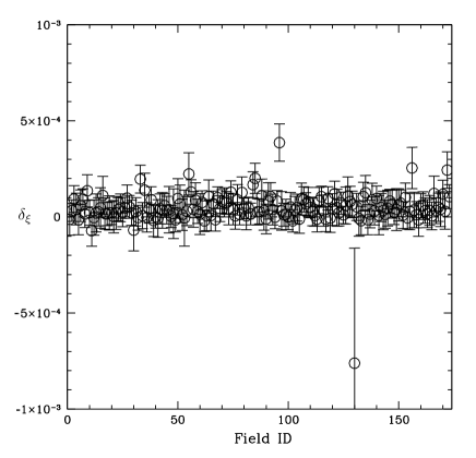
   Figure 6: Difference $\delta_{\xi}$ between shear autocorrelation $\xi_{+}$ and star–galaxy cross-correlation $\xi_{\rm sys}$ at scale $\theta=3\rm arcmin$. The difference delta of the S82p35p pointing is higher than others.

3. Two-point shear correlation functions. We calculate the two-point shear correlation functions of the shear catalogue and compare them to an analytical prediction. The comparison between the analytical prediction of halo model and the measured $\xi_{+}$ is good; see Fig. 7. Note the cross-correlation $\xi_{\rm tx}$ between the tangential and rotated shear should be zero. The theory appears to be systematically higher than the observation. This is due to the photometric redshift sample incompleteness.

   

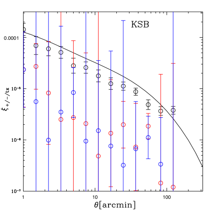
   Figure 7: The two-point shear correlation functions of the shear catalogue: $\xi_{+}$ (black points), $\xi_{-}$ (red points), and $\xi_{\rm tx}$ (blue points). Solid lines show the analytical predictions of $\xi_{+}$. Note the cross-correlation $\xi_{\rm tx}$ between the tangential and rotated shear should be zero. The solid line is the theoretical prediction for a WMAP7 cosmology.

4. $E,B$-mode signals. We test for the (nonphysical) $B$-mode signal. The $B$-mode signal corresponds to the imaginary component of $P_{\kappa}(\ell)$. We rotate all galaxy shears through $45^{\circ}$ and remeasure the $E$-mode signal. We measure that the $B$-mode signals are around zero except for small scales; see Fig. 8.

   

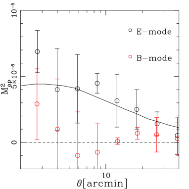
   Figure 8: The aperture mass from the entire CFHT/Stripe 82 field. Red points show the B-mode, black points show the E-mode. The error bars of the E-mode include statistical noise added in quadrature to the non-Gaussian cosmic variance. Only statistical uncertainty contributes to the error budget for the B-mode. The errorbars are $1\sigma$ confidence level. Within $2\sigma$ errors the B-modes are consistent with zero. The solid line is the theoretical prediction for a WMAP 7-cosmology.

For the lensing catalogue, we only select galaxies fainter than the foreground samples by 1 mag in $i$ band, so that we have no overlap between the two samples. The complete redshift distribution of the sources used for the WL analysis is displayed in Fig. 1 with a thick dashed black line labelled ‘background sources’.

4 Measurements

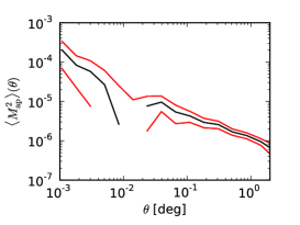
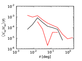
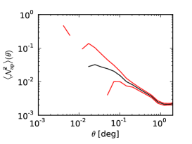
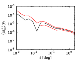
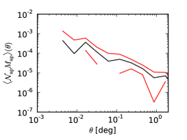
Figure 11: WL measurements for the LRG-WISE bright (top row) faint (bottom row) sample. From the left to the right the galaxy autocorrelation $\mathcal{N}^{2}(\theta)$, the matter autocorrelation $M_{\mathrm{ap}}^{2}(\theta)$, and the galaxy–matter cross-correlation $\mathcal{N}(\theta)M_{\mathrm{ap}}(\theta)$. The black line represents the mean value and the red lines the $1\sigma$ error contours. Measurements of $M_{\mathrm{ap}}^{2}(\theta)$ and $\mathcal{N}^{2}(\theta)$ are clean for $\theta>0.06^{\circ}$ for both samples. $\mathcal{N}(\theta)M_{\mathrm{ap}}(\theta)$ is not.

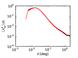
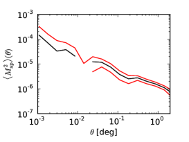
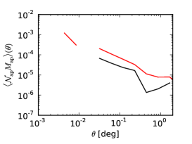
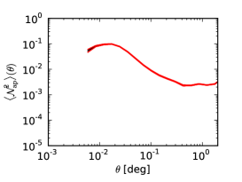
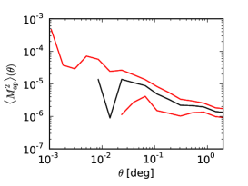
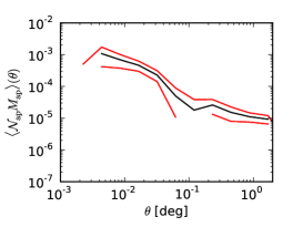
Figure 12: WL measurements for the gri ELG bright (top row) faint (bottom row) sample. From the left to the right the galaxy autocorrelation $\mathcal{N}^{2}(\theta)$, the matter autocorrelation $M_{\mathrm{ap}}^{2}(\theta)$, and the galaxy–matter cross-correlation $\mathcal{N}(\theta)M_{\mathrm{ap}}(\theta)$. The black line represents the mean value and the red lines the $1\sigma$ error contours. Measurements are clean between $0.1^{\circ}$ and $1^{\circ}$ for the $M_{\mathrm{ap}}^{2}(\theta)$ and $\mathcal{N}^{2}(\theta)$ of the bright sample and $\mathcal{N}^{2}(\theta)$ of the faint sample. The other lensing measurements are not robust.

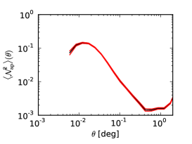
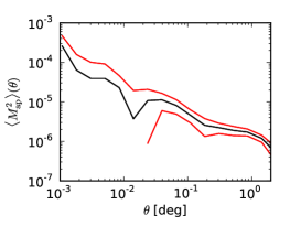
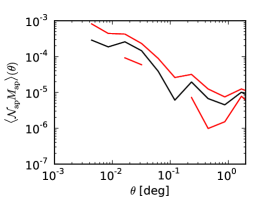
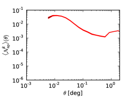
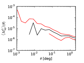
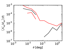
Figure 13: WL measurements for the ugri ELG bright (top row) faint (bottom row) sample. From the left to the right the galaxy autocorrelation $\mathcal{N}^{2}(\theta)$, the matter autocorrelation $M_{\mathrm{ap}}^{2}(\theta)$, and the galaxy–matter cross-correlation $\mathcal{N}(\theta)M_{\mathrm{ap}}(\theta)$. The black line represents the mean value and the red lines the $1\sigma$ error contours. Measurements are clean between $0.05^{\circ}$ and $1^{\circ}$ for the $M_{\mathrm{ap}}^{2}(\theta)$ and $\mathcal{N}^{2}(\theta)$ of the bright sample and $\mathcal{N}^{2}(\theta)$ of the faint sample. The other lensing measurements are not robust.

In this section, we present the measurements made through clustering and WL analysis of the data. The correlation function measurements are displayed in Figs 9-13. Figs 14 and 15 show the galaxy bias measurement. Table 3 summarizes the details of the measurements.

4.1 Angular clustering measure and HOD fits

We measure the angular clustering, denoted $w(\theta)$, for angles in the range 0.001^∘ to 1.5^∘. In this manner we avoid the signal due to blended sources. In the case of LRG-WISE, the clustering analysis starts at 0.01^∘. We use between 15 and 20 angular bins regularly log-spaced. The errors and the covariance matrix are issued from 112 bootstrap realizations of the angular clustering measure. Fig. 9 shows a comparison of the angular clustering of all previously defined samples.

The most precise estimations of the angular correlation functions are between 0.01^∘ and 0.1^∘, due to a balance between the density of BAO tracers and the geometry of the survey. For the sparse tracers (the bright selections at low redshift), below 0.01^∘, there are only a few pairs of tracers. For the densest tracers, the correlation function is precise down to 0.001^∘. For all tracers above 0.1^∘, given the geometry of the survey (a long stripe), the correlation function measurements are covariant. We correct from the integral constraint as in Wall & Jenkins (2012).

The main trends in the angular clustering measurements follow expectations. The lower redshift samples are more clustered than higher redshift samples. The bright samples are more clustered than the faint samples in particular at small scales.

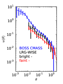
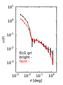
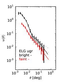
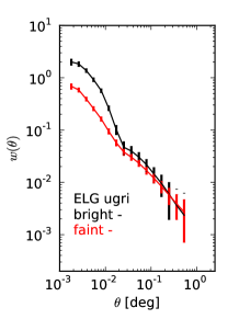
Figure 9: Angular clustering of the selected tracers. The wide angular span of the clustering allows the HOD analysis, except for the LRG-WISE, that are limited to $\theta>0.01^{\circ}$.

To interpret the angular clustering, we use the HOD parametrization given in (2). From $N(M)$ we deduce the angle averaged 3D correlation function, that we project using the Limber equation (Limber, 1954; Simon, 2007) to obtain the angular autocorrelation function $w_{\mathrm{HOD}}$. The $\chi^{2}$ accounting for the accuracy of the fit is defined by equation (11):

$$\chi^{2}=(w_{\mathrm{observed}}-w_{\mathrm{HOD}})^{\mathrm{T}}C^{-1}(w_{\mathrm{observed}}-w_{\mathrm{HOD}})+\frac{(N^{\mathrm{gal}}_{\mathrm{mes}}-N^{\mathrm{gal}}_{\mathrm{mes}})^{2}}{\sigma^{2}_{\mathrm{Ngal}}}.$$ (11)

The main source of error is the uncertainty on the number of galaxies representing the redshift distribution of each population. This uncertainty lies between 5 and 20 per cent for the bright tracers (CMASS and ELG bright). For the faint tracers it is between 30 and 40 per cent (error denoted $\sigma_{\mathrm{Ngal}}$). The second source of errors is the statistical errors on the measurement of $w(\theta)$, which is accounted for by the covariance matrix $C$. Another source of errors is the cosmic variance, but it is small compared to other uncertainty sources. The fractional error on the measured density due to cosmic variance is $\sigma_{\mathrm{cv}}<0.1$; see Newman & Davis (2002). We account for these when computing the error on the HOD derived parameters; see Table 3.

We perform additional tests to search for systematic errors. We test if the angular clustering measured is representative of the redshift distribution. We compute the angular clustering on only the tracers that have a reliable photoZ. We find a discrepancy on the angular clustering smaller by a factor of three than the statistical error on the angular clustering measurement. We therefore assume the angular clustering measurement is representative of the redshift distribution.

The validity of the use of an HOD model can be discussed. $N(M)$ is valid to predict the clustering when applied to a volume-limited sample. Current data does not allow us to construct a clean volume-limited sample, as we do not have good photometric redshifts for all the tracers. We cannot cut a clean sample with redshift $z\in\bar{z}\pm\sigma_{z}$. We quantify the impact of the wide redshift distribution on the angular clustering on large scale, where it matters for the determination of the galaxy bias, using the Multidark simulation. We compare the angular clustering of haloes SHAM selected with a top-hat redshift distribution (1 if $z\in\bar{z}\pm\sigma_{z}$, else 0) and the observed redshift distribution. The large-scale angular clustering $\theta>0.08^{\circ}$ is unchanged. The small-scale angular clustering does change. Therefore we assume the large-scale angular clustering measured on the full sample is representative of the sample located in $\bar{z}\pm\sigma_{z}$, and that the bias, within the error bars will be correct. The values of the galaxy bias derived by the HOD method are given in Table 3 and plotted in Figs 14 and 15. This shows the major flaw of this HOD parametrization that cannot account for a galaxy population with a wide redshift distribution. A hint to try and model this would be to introduce a redshift dependence for the parameters describing $N(M)$. We further discuss this issue in section 5.

4.2 Weak lensing measurements

We measure $\mathcal{N}(\theta)M_{\mathrm{ap}}(\theta)$, $\mathcal{N}^{2}(\theta)$, $M_{\mathrm{ap}}^{2}(\theta)$ with the same routines as in Jullo et al. (2012). The SNR obtained on the bias is $\sim 3$ for tracers with $z<1$ and of $\sim 1.5$ for $z>1$. Because of this low SNR measurement, we exclude the ugr ELG sample at $z\simeq 1.2$ from the WL analysis. The measurements are shown in Figs 10 (CMASS), 11 (LRG-WISE), 12 (gri ELG) and 13 (ugri ELG). We derive the galaxy bias for all these samples; see Table 3. The cross-correlation $\mathcal{N}(\theta)M_{\mathrm{ap}}(\theta)$ is measured with precision only for the lower redshift CMASS sample. Therefore $r$ is computed only for this sample.

The main source of error arises from the error on the shape measurement; see the data description section. The uncertainty on the redshift distribution can also potentially introduce some systematic errors. All statistical errors are propagated with bootstrap as described in Jullo et al. (2012). For each foreground and background galaxy catalogue, 100 samples are randomly drawn and processed to compute the aperture auto- and cross-correlation functions as well as the bias and correlation coefficient. The background source catalogues are cut at 1 mag fainter than the foreground. Systematic error on $M_{\mathrm{ap}}^{2}(\theta)$ on large scale due to the lack of information at small scale is below $1$ per cent (Kilbinger et al., 2006).

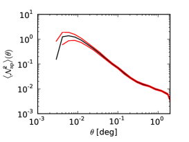
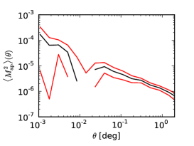
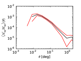
Figure 10: WL measurements for the BOSS-CMASS sample. From the left to the right the galaxy autocorrelation $\mathcal{N}^{2}(\theta)$, the matter autocorrelation $M_{\mathrm{ap}}^{2}(\theta)$, and the galaxy–matter cross-correlation $\mathcal{N}(\theta)M_{\mathrm{ap}}(\theta)$. The black line represents the mean value and the red lines the $1\sigma$ error contours. Measurements of $\mathcal{N}^{2}(\theta)$ and $M_{\mathrm{ap}}^{2}(\theta)$ are clean between $0.05^{\circ}$ and $1^{\circ}$. $\mathcal{N}(\theta)M_{\mathrm{ap}}(\theta)$ is clean between $0.02^{\circ}$ and $0.2^{\circ}$. We thus can deduce $b_{\mathrm{g}}$ and $r$.

4.3 Cross-correlation coefficient and galaxy bias

Measurements of the galaxy clustering as a function of the luminosity were performed in the local universe by (Coil et al., 2008), (Skibba & Sheth, 2009), (Zehavi et al., 2011) and (Guo et al., 2013). They showed the clustering amplitude is greater for more luminous samples. Thus we expect to measure high values of the galaxy bias for all samples. There is no straightforward existing relation that can predict the expected galaxy bias.

4.3.1 Cross-correlation coefficient

We measure the cross-correlation coefficient only for the CMASS sample, $r=1.16\pm 0.35$. This measurement is a first, and implies the CMASS galaxies are fully correlated with the matter field. This strongly supports current BAO analysis made on this sample (Anderson et al., 2012).

With current data, it is not possible to constrain the cross-correlation coefficient of the other galaxy samples.

4.3.2 Galaxy bias

For the CMASS, LRG-WISE bright, gri ELG bright, and ugri ELG bright samples, the measurements of the two methods are in agreement; see Fig. 14. We find the bias is above $1.5$ for the all ELG selections, which is consistent with the measurements made by Coupon et al. (2012) and Mostek et al. (2013) on their brightest samples. We consider both measurements give a trend about the size of dark matter haloes these galaxies inhabit; see Fig. 15. Comparing the values of the bias with the curves of the bias for a constant halo mass after Tinker et al. (2005) and with the mass distributions obtained via SHAM shows all these samples are tracing the most massive haloes at their respective redshifts. From Fig. 14 we note that the bias from the HOD seems systematically higher than that of WL. The bias of the HOD corresponds to the bias of a sample that is complete in mass (represented by $N(M)$). Though the assumption of completeness in mass does not really hold for clue colour-selected samples. The bias output by the WL does not need this assumption, and is thus lower than the value obtained via the HOD and probably closer to the reality for the bright samples where SNR is sufficient. We think this is the primary reason to this systematic discrepancy. With current data, it is not possible to estimate precisely stellar masses and understand this discrepancy in greater details.

For the LRG-WISE faint, gri ELG faint and ugri ELG faint samples, there is a systematic disagreement between the methods: the clustering analysis outputs a higher bias than the WL analysis; see Fig. 14. Thus for the LRG-WISE faint, gri ELG faint and ugri ELG faint samples, we find the combination of current surveys ”CFHT/Stripe 82 + CFHT-LS + SDSS-S82 deep co-add” is too shallow to derive a reliable value of the bias. We need a fair spectroscopic sample of such tracers to improve the photometric redshift distribution accuracy, and a deeper survey for the shape of background galaxies.

For the ugr ELG bright (and faint), with current data, the WL analysis is not feasible. The galaxy bias derived using only the clustering information is although of prime interest. It is consistent with the fact that the ugr ELG bright sample occupies the most massive haloes at $z\sim 1.2$.

4.3.3 Satellite fraction, halo mass and HOD

The shape of the angular clustering for the ELG samples suggests a high satellite fraction. Indeed there is a strong bump for $\theta<0.02^{\circ}$. The HOD models fail to reproduce trustworthy satellite fractions for the ELG samples; see Table 3. For the CMASS sample, that is approximately complete in mass and a volume-limited sample, HOD and SHAM methods are in agreement and obtain 5 per cent of satellites. For the $gri$ ELG sample, which is the reddest of the ELG samples, the HOD and SHAM satellite fractions are in agreement, but remain below 10 per cent. Given the observed small-scale bump, we expected satellite fraction of the order of 15-25 per cent. For the $ugri$ and the $ugr$ ELG samples, the satellite fractions do not really make sense. They are not consistent between the bright and the faint sample, which is puzzling. It shows the HOD models have a high degeneracy when they fit the small angular scales of a sample with a wide redshift distribution. A similar effect is seen for the mean halo mass predicted by the HOD; it is always 0.5 dex higher than the expectations set by the SHAM. The clustering curves of the brightest galaxies in each redshift bin therefore constitute a new challenge to halo occupation models.

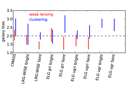
Figure 14: Large-scale galaxy bias of the different BAO tracers ordered by mean redshift. The bright samples are more biased than the faint samples. The HOD bias is not in agreement for the faint samples and tends to be greater than the WL estimation.

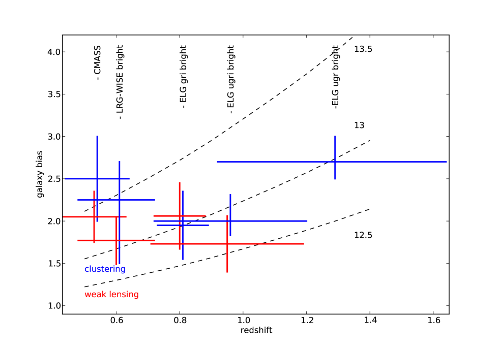
Figure 15: Large-scale galaxy bias of the different BAO tracers vs. redshift. The interquartile are shown as error bars (25 per cent - 75 per cent intervals). The dashed black lines correspond to the bias of haloes of mass $\log_{10}{M_{\mathrm{200}}/M\odot}$ of 12.5, 13 and 13.5 from bottom to the top, after Tinker et al. (2005). The figure shows the ELGs inhabit haloes of mass between $10^{12.5}$ and $10^{13}M\odot$. The comparison with the SHAM halo mass values (Table 2) shows these selections are tracing the most massive haloes at their mean redshift.

Table 3: Results from the clustering and the WL analysis. The number of degrees of freedom is $\sim 18$ for the HOD fits. The values of the $\chi^{2}$ show current HOD models fail in explaining angular clustering of the ELGs. The column $\leftrightarrow M_{\mathrm{d}}$ states the relation $M_{\mathrm{halo}}-M_{\mathrm{d}}$. $b_{\mathrm{clustering}}$ is the galaxy bias obtained with the HOD, $\langle b_{\mathrm{WL}}\rangle$ with the WL, and $\langle r_{\mathrm{WL}}\rangle$ is cross-correlation coefficient. The column satellite fraction compares the results from the SHAM and the HOD.

Sample	Maximum likelihood HOD parameter					$\chi^{2}/$dof	Halo mass		Satellite fraction		$b_{\mathrm{clustering}}$	$\langle b_{\mathrm{WL}}\rangle$	$\langle r_{\mathrm{WL}}\rangle$
	$log(\frac{M_{min}}{M\odot})$	$log(\frac{M_{1}}{M\odot})$	$log(\frac{M_{0}}{M\odot})$	$\sigma_{logM}$	$\alpha$		$\langle M_{halo}\rangle$	$\leftrightarrow M_{\mathrm{d}}$	HOD	SHAM
CMASS	13.433	14.576	10.73	0.242	1.790	0.3012	13.779	$>$	5	5	$2.5\pm 0.5$	$2.05\pm 0.3$	$1.16\pm 0.35$
LRG-WISE bright	-	-	-	-	-	-	-	-	-	4	$2.25^{+0.5}_{-0.7}$	$1.77\pm 0.28$	-
LRG-WISE faint	-	-	-	-	-	-	-	-	-	7	$2.0\pm 0.2$	$1.44\pm 0.22$	-
ELG gri bright	13.51	14.51	11.07	0.89	0.81	16.05	13.219	$=$	6	8	1.95$\pm 0.4$	$2.06\pm 0.39$	-
ELG gri faint	13.256	14.931	11.994	0.268	0.691	3.379	13.558	$>$	9	10	$2.5^{+0.7}_{-0.3}$	$1.57\pm 0.38$	-
ELG ugri bright	12.41	12.043	12.422	0.58	0.64	2.88	13.157	$=$	52	7	$2.0^{+0.31}_{-0.17}$	$1.73\pm 0.33$	-
ELG ugri faint	13.049	14.443	13.089	0.69	0.54	6.95	13.084	$>$	5	11	$2.1^{+0.5}_{-0.2}$	$1.56\pm 0.34$	-
ELG ugr bright	13.179	13.409	13.074	0.63	0.62	1.54	13.241	$<$	16	3	$2.7^{+0.3}_{-0.2}$	-	-
ELG ugr faint	13.103	14.386	12.928	0.592	0.779	6.53	13.126	$=$	4	7	$2.5^{+0.5}_{-0.2}$	-	-

5 Discussion

The measurements presented in this paper are meaningful only for the CMASS, LRG-WISE bright, gri ELG bright, ugri ELG bright, and ugr ELG bright (clustering only) samples. The following discussion is therefore restricted to these tracers unless otherwise stated (we set aside the ELG faint samples).

5.1 Are these selections suitable for future BAO studies ?

The SNR in BAO goes as the number density ($\bar{n}$) times the power spectrum, which amplitude scales as the square of the galaxy bias $b^{2}$ for a constant $\sigma_{8}$. Thus $\mathrm{SNR_{BAO}}\propto\bar{n}P\propto\bar{n}b^{2}$. Thus the higher the bias (or the amplitude, it is equivalent), the smaller is the number density required to a reach a given SNR, and thus the faster the survey. For the same SNR, the density required using tracers with $b=1.5$ (respectively $b=2$) is 2.25 (respectively 4) times smaller than using tracers with a bias $b=1$. A BAO survey using these tracers has thus a real advantage compared to selecting galaxies with lower absolute luminosity that have a lower clustering amplitude. These numbers constitute a zeroth order value of the galaxy bias that can be used in simulation to predict the accuracy of the detection and anticipate the requirements on geometry and density for surveys as SDSS-IV/eBOSS, DESspec, BigBOSS, PFS-SuMiRe, and Euclid. A check could be performed with n-body simulations by trying to reproduce the angular clustering measurements from this paper.

The primary role of the target selection, to select highly-biased galaxies, is here fulfilled. There is, however, a trade-off. The galaxy bias is the source of the dominating systematic on the BAO measurement; see Mehta et al. (2011) and references therein. With current reconstruction algorithms, and a knowledge of the bias better than 10 per cent, simulations show it is possible to reduce the systematic errors down to 0.15 per cent. This study enables to start calibrating simulations on observed data to understand how to cope with this systematic effect.

5.2 Sensitivity to input cosmological parameters

In this study, we use WMAP7 fiducial values for cosmological parameters, yet the latest parameters obtained by Planck differ slightly, see Planck Collaboration et al. (2013). The mean change of the angular correlation function of matter on linear scales (between $0.05^{\circ}$ and $0.5^{\circ}$) at $z\sim 0.8$ with the redshift distribution of the bright $gri$ ELG is of $\sim 7$ per cent. The WMAP parameters predict a matter clustering stronger by $\sim 7$ per cent than that of Planck. Therefore with Planck parameters, the galaxy bias would increase by $\sim 3.5$ per cent compared to the values we measure here.

5.3 Complementarity of the lower redshift selections

The redshift distribution of the CMASS, LRG-WISE and gri ELG are overlapping in $0.6<z<0.7$; see Fig. 1. The match between the catalogues shows that 20 per cent of the tracers are common between the LRG-WISE bright sample and the CMASS. There is no common tracers between the $gri$ ELG and the LRG-WISE bright or the CMASS. These three samples are therefore complementary to map the large scale structures in this redshift zone, and particularly to perform cross-correlation analysis.

5.4 ELG $ugri$ selection, an intermediate selection

The ugri ELG colour selection is a hybrid between the ugr and the gri selections. The clustering analysis shows the $w(\theta)$ of the ugri is located between that of the ugr and the $gri$ $w(\theta)$. It is thus consistent.

5.5 Hints on luminosity, stellar mass, halo mass, HOD modelling and $N$-body simulations

Wake et al. (2011) showed that stellar mass and halo mass are correlated for $1<z<2$, and Li et al. (2006) reported that on large scales the galaxy clustering amplitude dependence on stellar mass is positively correlated to the luminosity. Our selections target the most luminous galaxies (in their redshift range). We therefore expect to track high stellar masses and high halo masses. The combination of the clustering analysis from this work and of the estimates of stellar masses from Comparat et al. (2013) demonstrate that these galaxies trace haloes with large masses ($M_{halo}\sim 10^{12.5}-10^{13}M\odot$), i.e. we comply with the general picture.

This analysis is complementary to similar analyses based on faint and deep ‘pencil beam’ surveys, that investigate the clustering properties of average luminosity galaxies, see Leauthaud et al. (2012) and Mostek et al. (2013). In fact our target selections aim for galaxies that are not in large numbers in such surveys. Given the trends in these papers, our results are in good agreement with what galaxy bias is expected for the brightest galaxies at redshift $z=1$.

These clustering measurements are the first of its kind and are of prime interest to improve our knowledge of the halo occupation distribution of such galaxy populations. In this work, we assumed the angular clustering measured was representative of the clustering of a volume-limited sample at the mean redshift of the sample in order to derive its large scale bias. This assumption is not simple to test with current data, in particular with current photometric redshifts. Though this might be one of the reasons why the HOD model fails to describe in details the observed angular clustering at small scales, in particular the satellite fractions. In fact the properties of the selected galaxies evolve with redshift i.e. the lower redshift ones are less luminous than the higher redshift ones. The HOD model used here does not have parameters that evolve with redshift, it is a fixed halo population convolved with the redshift distribution. These considerations are oriented towards the construction of a mock catalogue.

6 Conclusion

We measured, for the first time, the angular clustering and the cosmic shear of the future samples selected for BAO studies. We have validated the use of this method on the CMASS sample as our measurement agrees with previous results. Moreover, we show that the CMASS sample is well correlated to the dark matter field.

We demonstrate that the bright ELG samples are highly biased and therefore suited to detect BAO. The galaxies to be targeted for the near future SDSS-IV/eBOSS BAO experiment will provide a high SNR in the galaxy power spectrum.

This work provides a strong basis to develop simulations and mock catalogues of these galaxy populations in order to understand the details of the relation ELG - dark matter haloes.

When pushing the method further in depth (ELG faint samples), we are limited by the knowledge of the redshift distribution of the tracers and by the depth of galaxy shape catalogues for WL. Both methods disagree when the redshift distribution is poorly known, i.e., with an uncertainty of about 40 per cent. Within the next few years, deeper observations and improved photometric redshifts should provide the necessary data to describe with precision the relation between galaxies and matter probed by the faint target selection schemes.

References

- Ahn et al. (2012) Ahn C. P. et al., 2012, ApJS, 203, 21
- Anderson et al. (2012) Anderson L. et al., 2012, MNRAS , 427, 3435
- Annis et al. (2011) Annis J. et al., 2011, ArXiv e-prints
- Bacon et al. (2003) Bacon D. J., Massey R. J., Refregier A. R., Ellis R. S., 2003, MNRAS , 344, 673
- Beutler et al. (2011) Beutler F. et al., 2011, MNRAS , 416, 3017
- Blake et al. (2011) Blake C. et al., 2011, MNRAS , 415, 2892
- Boulade et al. (2003) Boulade O. et al., 2003, in Society of Photo-Optical Instrumentation Engineers (SPIE) Conference Series, Vol. 4841, Society of Photo-Optical Instrumentation Engineers (SPIE) Conference Series, Iye M., Moorwood A. F. M., eds., pp. 72–81
- Bridle et al. (2010) Bridle S. et al., 2010, MNRAS , 405, 2044
- Busca et al. (2013) Busca N. G. et al., 2013, A&A , 552, A96
- Cacciato et al. (2012) Cacciato M., Lahav O., van den Bosch F. C., Hoekstra H., Dekel A., 2012, MNRAS , 426, 566
- Capak et al. (2007) Capak P. et al., 2007, ApJS, 172, 99
- Coil et al. (2008) Coil A. L. et al., 2008, Astrophys. J. , 672, 153
- Comparat et al. (2013) Comparat J. et al., 2013, MNRAS , 428, 1498
- Conroy et al. (2006) Conroy C., Wechsler R. H., Kravtsov A. V., 2006, Astrophys. J. , 647, 201
- Cooray & Sheth (2002) Cooray A., Sheth R., 2002, Physics Letters B, 372, 1
- Coupon et al. (2009) Coupon J. et al., 2009, A&A , 500, 981
- Coupon et al. (2012) Coupon J. et al., 2012, A&A , 542, A5
- Dawson et al. (2013) Dawson K. S. et al., 2013, AJ , 145, 10
- Dekel & Lahav (1999) Dekel A., Lahav O., 1999, Astrophys. J. , 520, 24
- Drinkwater et al. (2010) Drinkwater M. J. et al., 2010, MNRAS , 401, 1429
- Eisenstein & Hu (1998) Eisenstein D. J., Hu W., 1998, Astrophys. J. , 496, 605
- Eisenstein et al. (2011) Eisenstein D. J. et al., 2011, AJ , 142, 72
- Erben et al. (2012) Erben T. et al., 2012, ArXiv e-prints
- Frieman et al. (2008) Frieman J. A., Turner M. S., Huterer D., 2008, Annual Review of Astronomy and Astrophysics, 46, 385
- Fukugita et al. (1996) Fukugita M., Ichikawa T., Gunn J. E., Doi M., Shimasaku K., Schneider D. P., 1996, AJ , 111, 1748
- Gunn et al. (1998) Gunn J. E. et al., 1998, AJ , 116, 3040
- Gunn et al. (2006) Gunn J. E. et al., 2006, AJ , 131, 2332
- Guo et al. (2013) Guo H. et al., 2013, Astrophys. J. , 767, 122
- Heymans et al. (2006a) Heymans C. et al., 2006a, MNRAS , 368, 1323
- Heymans et al. (2012) Heymans C. et al., 2012, MNRAS , 427, 146
- Heymans et al. (2006b) Heymans C., White M., Heavens A., Vale C., van Waerbeke L., 2006b, MNRAS , 371, 750
- Hoekstra et al. (2002) Hoekstra H., van Waerbeke L., Gladders M. D., Mellier Y., Yee H. K. C., 2002, Astrophys. J. , 577, 604
- Huff et al. (2011) Huff E. M., Hirata C. M., Mandelbaum R., Schlegel D., Seljak U., Lupton R. H., 2011, ArXiv e-prints
- Ilbert et al. (2006) Ilbert O. et al., 2006, A&A , 457, 841
- Ilbert et al. (2009) Ilbert O. et al., 2009, Astrophys. J. , 690, 1236
- Jones et al. (2009) Jones D. H. et al., 2009, MNRAS , 399, 683
- Jullo et al. (2012) Jullo E. et al., 2012, Astrophys. J. , 750, 37
- Kaiser (1984) Kaiser N., 1984, ApJ, 284, L9
- Kaiser et al. (1995) Kaiser N., Squires G., Broadhurst T., 1995, Astrophys. J. , 449, 460
- Kilbinger et al. (2011) Kilbinger M. et al., 2011, ArXiv e-prints
- Kilbinger et al. (2009) Kilbinger M. et al., 2009, A&A , 497, 677
- Kilbinger et al. (2006) Kilbinger M., Schneider P., Eifler T., 2006, A&A , 457, 15
- Kilbinger et al. (2010) Kilbinger M. et al., 2010, MNRAS , 405, 2381
- Kirkby et al. (2013) Kirkby D. et al., 2013, JCAP , 3, 24
- Kitching et al. (2012) Kitching T. D. et al., 2012, MNRAS , 423, 3163
- Komatsu et al. (2011) Komatsu E. et al., 2011, ApJS, 192, 18
- Kravtsov et al. (2004) Kravtsov A. V., Berlind A. A., Wechsler R. H., Klypin A. A., Gottlöber S., Allgood B., Primack J. R., 2004, Astrophys. J. , 609, 35
- Landy & Szalay (1993) Landy S. D., Szalay A. S., 1993, Astrophys. J. , 412, 64
- Laureijs et al. (2011) Laureijs R. et al., 2011, ArXiv e-prints
- Leauthaud et al. (2010) Leauthaud A. et al., 2010, Astrophys. J. , 709, 97
- Leauthaud et al. (2011) Leauthaud A., Tinker J., Behroozi P. S., Busha M. T., Wechsler R. H., 2011, Astrophys. J. , 738, 45
- Leauthaud et al. (2012) Leauthaud A. et al., 2012, Astrophys. J. , 744, 159
- Lee et al. (2013) Lee K.-G. et al., 2013, AJ , 145, 69
- Li et al. (2006) Li C., Kauffmann G., Jing Y. P., White S. D. M., Börner G., Cheng F. Z., 2006, MNRAS , 368, 21
- Limber (1954) Limber D. N., 1954, Astrophys. J. , 119, 655
- Luppino & Kaiser (1997) Luppino G. A., Kaiser N., 1997, Astrophys. J. , 475, 20
- Ma & Fry (2000) Ma C.-P., Fry J. N., 2000, Astrophys. J. , 543, 503
- Massey et al. (2007) Massey R. et al., 2007, MNRAS , 376, 13
- Mehta et al. (2011) Mehta K. T., Seo H.-J., Eckel J., Eisenstein D. J., Metchnik M., Pinto P., Xu X., 2011, Astrophys. J. , 734, 94
- More et al. (2013) More S., van den Bosch F. C., Cacciato M., More A., Mo H., Yang X., 2013, MNRAS , 430, 747
- Mostek et al. (2013) Mostek N., Coil A. L., Cooper M., Davis M., Newman J. A., Weiner B. J., 2013, Astrophys. J. , 767, 89
- Newman & Davis (2002) Newman J. A., Davis M., 2002, Astrophys. J. , 564, 567
- Nuza et al. (2013) Nuza S. E. et al., 2013, MNRAS
- Oke & Gunn (1983) Oke J. B., Gunn J. E., 1983, Astrophys. J. , 266, 713
- Pâris et al. (2012) Pâris I. et al., 2012, A&A , 548, A66
- Parkinson et al. (2012) Parkinson D. et al., 2012, Phys. Rev. D , 86, 103518
- Planck Collaboration et al. (2013) Planck Collaboration et al., 2013, ArXiv e-prints
- Prada et al. (2012) Prada F., Klypin A. A., Cuesta A. J., Betancort-Rijo J. E., Primack J., 2012, MNRAS , 423, 3018
- Riebe et al. (2011) Riebe K. et al., 2011, ArXiv e-prints
- Schlegel et al. (2011) Schlegel D. et al., 2011, ArXiv e-prints
- Schneider et al. (1998) Schneider P., van Waerbeke L., Mellier Y., Jain B., Seitz S., Fort B., 1998, A&A , 333, 767
- Scoville et al. (2007) Scoville N. et al., 2007, ApJS, 172, 1
- Seljak (2000) Seljak U., 2000, MNRAS , 318, 203
- Shan et al. (2012) Shan H. et al., 2012, Astrophys. J. , 748, 56
- Sheth et al. (2001) Sheth R. K., Mo H. J., Tormen G., 2001, MNRAS , 323, 1
- Sheth & Tormen (1999) Sheth R. K., Tormen G., 1999, MNRAS , 308, 119
- Simon (2007) Simon P., 2007, A&A , 473, 711
- Simon et al. (2007) Simon P., Hetterscheidt M., Schirmer M., Erben T., Schneider P., Wolf C., Meisenheimer K., 2007, A&A , 461, 861
- Skibba & Sheth (2009) Skibba R. A., Sheth R. K., 2009, MNRAS , 392, 1080
- Slosar et al. (2013) Slosar A. et al., 2013, JCAP , 4, 26
- Smith et al. (2003) Smith R. E. et al., 2003, MNRAS , 341, 1311
- Suzuki et al. (2012) Suzuki N. et al., 2012, Astrophys. J. , 746, 85
- Tegmark & Bromley (1999) Tegmark M., Bromley B. C., 1999, ApJ, 518, L69
- Tegmark & Peebles (1998) Tegmark M., Peebles P. J. E., 1998, ApJ, 500, L79
- Tinker et al. (2005) Tinker J. L., Weinberg D. H., Zheng Z., Zehavi I., 2005, Astrophys. J. , 631, 41
- Trujillo-Gomez et al. (2011) Trujillo-Gomez S., Klypin A., Primack J., Romanowsky A. J., 2011, Astrophys. J. , 742, 16
- Vale & Ostriker (2004) Vale A., Ostriker J. P., 2004, MNRAS , 353, 189
- van den Bosch et al. (2013) van den Bosch F. C., More S., Cacciato M., Mo H., Yang X., 2013, MNRAS , 430, 725
- Wake et al. (2011) Wake D. A. et al., 2011, Astrophys. J. , 728, 46
- Wall & Jenkins (2012) Wall J. V., Jenkins C. R., 2012, Practical Statistics for Astronomers
- White et al. (2011) White M. et al., 2011, Astrophys. J. , 728, 126
- Wright et al. (2010) Wright E. L. et al., 2010, AJ , 140, 1868
- York et al. (2000) York D. G. et al., 2000, AJ , 120, 1579
- Zehavi et al. (2011) Zehavi I. et al., 2011, Astrophys. J. , 736, 59