A realistic distributed storage system: the rack model.

Abstract

In a realistic distributed storage environment, storage nodes are usually placed in racks, a metallic support designed to accommodate electronic equipment. It is known that the communication (bandwidth) cost between nodes which are in the same rack is much lower than between nodes which are in different racks.

In this paper, a new model, where the storage nodes are placed in two racks, is proposed and analyzed. Moreover, the two-rack model is generalized to any number of racks. In this model, the storage nodes have different repair costs depending on the rack where they are placed. A threshold function, which minimizes the amount of stored data per node and the bandwidth needed to regenerate a failed node, is shown. This threshold function generalizes the ones given for previous distributed storage models. The tradeoff curve obtained from this threshold function is compared with the ones obtained from the previous models, and it is shown that this new model outperforms the previous ones in terms of repair cost.

I Introduction

In a distributed storage environment, where the data is placed in nodes connected through a network, it is likely that one of these nodes fails. It is known that the use of erasure coding improves the fault tolerance and minimizes the amount of stored data per node [1], [2]. Moreover, the use of regenerating codes not only makes the most of the erasure coding improvements, but also minimizes the bandwidth needed to regenerate a failed node [3].

In realistic distributed storage environments, for example a storage cloud, the data is placed in storage devices which are connected through a network. These storage devices are usually organized in a rack, a metallic support designed to accommodate electronic equipment. The communication (bandwidth) cost between nodes which are in the same rack is much lower than between nodes which are in different racks. In fact, in [4] it is said that reading from a local disk is nearly as efficient as reading from the disk of another node in the same rack.

In [3], an optimal tradeoff given by a threshold function between the amount of stored data per node and the bandwidth needed to regenerate a failed node (repair bandwidth) in a distributed storage environment was claimed. This tradeoff was proved by using the mincut on information flow graphs, and it can be represented as a curve, where the two extremal points of the curve are called the Minimum Storage Regenerating (MSR) point and the Minimum Bandwidth Regenerating (MBR) point.

In [5], another model, where there is a static classification of the storage nodes in two sets: one with the “cheap bandwidth” nodes, and another one with the “expensive bandwidth” nodes, was presented and analyzed. This classification of the nodes is not based on racks, because the nodes in the expensive set are always expensive in terms of the cost of sending data to a newcomer, regardless of the specific newcomer. A description of this model is included in Subsection II-B. There are other models, usually called non-homogeneous, which are based on one or more nodes being able to store different amounts of data. Examples of these models are presented in [6] and [7].

This paper is organized as follows. In Section II, we review previous distributed storage models in order to present the new model in next section. In Section III, we start by describing this new model where the storage nodes are placed in two racks. We also provide a general threshold function, and we describe the extremal Minimum Storage and Minimum Bandwidth Regenerating points. In Section IV, we generalize the two-rack model to any number of racks. In Section V, we analyze the results obtained from this new model by comparing them with the previous models. Finally, in Section VI, we expose the conclusions of this study.

II Previous models

In this section, we describe the previous distributed storage models: the basic model and the static cost model introduced in [3] and [5], respectively.

II-A Basic model

In [3], Dimakis et al. introduced a first distributed storage model, where each storage node has the same repair bandwidth. Moreover, the fundamental tradeoff between the amount of stored data per node and the repair bandwidth was given from analyzing the mincut of an information flow graph.

Let $C$ be a $[n,k,d]$ regenerating code composed by $n$ storage nodes, each one storing $\alpha$ data units, and such that any $k$ of these $n$ storage nodes contain enough information to recover the file. In order to be able to recover a file of size $M$, it is necessary that $\alpha k\geq M$. When one node fails, $d$ of the remaining $n-1$ storage nodes send $\beta$ data units to the new node which replaces the failed one. The new node is called newcomer, and the set of $d$ nodes sending data to the newcomer are called helper nodes. The total amount of bandwidth used per node regeneration is $\gamma=d\beta$.

Figure 1: Information flow graph corresponding to a $[4,2,3]$ regenerating code.

Let $s_{i}$, where $i=1,\ldots,\infty$, be the $i$-th storage node. Let $G(V,E)$ be a weighted graph designed to represent the information flow. Then, $G$ is in fact a directed acyclic graph, with a set of vertices $V$ and a set of arcs $E$. The set $V$ is composed by three kinds of vertices:

• Source vertex $S$: it represents the file to be stored. There is only one source vertex in the graph.

• Data collector vertex $DC$: it represents the user who is allowed to access the data in order to reconstruct the file.

• Storage node vertices $v_{in}^{i}$ and $v_{out}^{i}$: each storage node $s_{i}$, where $i=1,\ldots,\infty$, is represented by one inner vertex $v_{in}^{i}$ and one outer vertex $v_{out}^{i}$.

In general, there is an arc $(v,w)\in E$ of weight $c$ from vertex $v\in V$ to vertex $w\in V$ if $v$ can send $c$ data units to $w$.

At the beginning of the life of a distributed storage environment, there is a file to be stored in $n$ storage nodes $s_{i}$, $i=1,\ldots,n$. This can be represented by a source vertex $S$ with outdegree $n$ connected to vertices $v_{in}^{i}$, $i=1,\ldots,n$. Since we are interested in analyzing the information flow graph $G$ in terms of $\alpha$ and $\beta$, and these $n$ arcs are not significant to find the mincut of $G$, their weight is set to infinite. Moreover, to represent that each one of the storage nodes $s_{i}$, $i=1,\ldots,n$, stores $\alpha$ data units, each vertex $v_{in}^{i}$ is connected to the vertex $v_{out}^{i}$ with an arc of weight $\alpha$.

When the first storage node fails, the first newcomer $s_{n+1}$ connects to $d$ existing storage nodes sending, each one of them, $\beta$ data units. This can be represented by adding one arc from $v_{out}^{i}$, $i=1,\ldots,n$, to $v_{in}^{n+1}$ of weight $\beta$ if $s_{i}$ sends $\beta$ data units to $s_{n+1}$ in the regenerating process. The new vertex $v_{in}^{n+1}$ is also connected to its associated vertex $v_{out}^{n+1}$ with an arc of weight $\alpha$. This process can be repeated for every failed node. Let the newcomers be denoted by $s_{j}$, where $j=n+1,\ldots,\infty$.

Finally, after some failures, a data collector wants to reconstruct the file. Therefore, a vertex $DC$ is added to $G$ along with one arc from vertex $v_{out}^{i}$ to $DC$ if the data collector connects to the storage node $s_{i}$. Note that if $s_{i}$ has been replaced by $s_{j}$, the vertex $DC$ can not connect to $v_{out}^{i}$, but it can connect to $v_{out}^{j}$. The vertex $DC$ has indegree $k$ and each arc has weight infinite, because they have no relevance in finding the mincut of $G$.

If the mincut from vertex $S$ to $DC$, denoted by $\mbox{mincut}(S,DC)$, achieves that $\mbox{mincut}(S,DC)\geq M$, the data collector can reconstruct the file, since there is enough information flow from the source to the data collector. In fact, the data collector can connect to any $k$ nodes, so $\min(\mbox{mincut}(S,DC))\geq M$, which is achieved when the data collector connects to $k$ storage nodes that have been already replaced by a newcomer [3]. From this scenario, the mincut is computed and lower bounds on the parameters $\alpha$ and $\gamma$ are given. Let $\alpha^{*}(d,\gamma)$ be the threshold function, which is the function that minimizes $\alpha$. Since $\alpha\geq\alpha^{*}(d,\gamma)$, if $\alpha^{*}(d,\gamma)$ can be achieved, then any $\alpha\geq\alpha^{*}(d,\gamma)$ is also achieved.

Figure 1 illustrates the information flow graph $G$ associated to a $[4,2,3]$ regenerating code. Note that $\mbox{mincut}(S,DC)=\min(3\beta,\alpha)+\min(2\beta,\alpha)$ which is the minimum mincut for this information flow graph. In general, it can be claimed that $\mbox{mincut}(S,DC)\geq\sum_{i=0}^{k-1}\min((d-i)\beta,\alpha)\geq M$, which after an optimization process leads to the following threshold function $\alpha^{*}(d,\gamma)$ also shown in [3]:

$$\alpha^{*}(d,\gamma)=\left\{\begin{array}[]{ll}\frac{M}{k},&\gamma\in[f(0),+\infty)\\ \\ \frac{M-g(i)\gamma}{k-i},&\gamma\in[f(i),f(i-1))\\ &i=1,\ldots,k-1,\end{array}\right.$$ (1)

where

$$f(i)=\frac{2Md}{(2k-i-1)i+2k(d-k+1)}\text{ and }g(i)=\frac{(2d-2k+i+1)i}{2d}.$$

Using the information flow graph $G$, we can see that there are exactly $k$ points in the tradeoff curve, or equivalently, $k$ intervals in the threshold function $\alpha^{*}(d,\gamma)$, which represent $k$ newcomers. In the mincut equation, the $k$ terms in the summation are computed as the minimum between two parameters: the sum of the weights of the arcs that we have to cut to isolate the corresponding $v^{j}_{in}$ from $S$, and the weight of the arc that we have to cut to isolate the corresponding $v^{j}_{out}$ from $S$. Let the first parameter be called the income of the corresponding newcomer $s_{j}$. Note that the income of the newcomer $s_{j}$ depends on the previous newcomers.

It can be seen that the newcomers can be ordered according to their income from the highest to the lowest. In this model, this order is only determined by the order of replacement of the failed nodes. Moreover, the MSR point corresponds to the lowest income, which is given by the last newcomer added to the information flow graph; and the MBR point corresponds to the highest, which is given by the first newcomer. It is important to note also that, in this model, the order of replacement of the nodes does not affect to the final result, since the mincut is always the same independently of the specific set of $k$ failed nodes.

II-B Static cost model

In [5], Akhlaghi et al. presented another distributed storage model, where the storage nodes are partitioned into two sets $V^{1}$ and $V^{2}$. Let $V^{1}$ be the set of “cheap bandwidth” nodes, from where each data unit sent costs $C_{c}$, and $V^{2}$ be the set of “expensive bandwidth” nodes, from where each data unit sent costs $C_{e}$ such that $C_{e}>C_{c}$. This means that when a newcomer replaces a lost storage node, the cost of downloading data from a node in $V^{1}$ will be lower than the cost of downloading the same amount of data from a node in $V^{2}$.

Consider the same situation as in the model described in Subsection II-A. Now, when a storage node fails, the newcomer node $s_{j}$, $j=n+1,\ldots,\infty$, connects to $d_{c}$ existing storage nodes from $V^{1}$ sending each one of them $\beta_{c}$ data units to $s_{j}$, and to $d_{e}$ existing storage nodes from $V^{2}$ sending each one of them $\beta_{e}$ data units to $s_{j}$. Let $d=d_{c}+d_{e}$ be the number of helper nodes. Assume that $d$, $d_{c}$, and $d_{e}$ are fixed, that is, they do not depend on the newcomer $s_{j}$, $j=n+1,\ldots,\infty$. In terms of the information flow graph $G$, there is one arc from $v_{out}^{i}$ to $v_{in}^{j}$ of weight $\beta_{c}$ or $\beta_{e}$, depending on whether $s_{i}$ sends $\beta_{c}$ or $\beta_{e}$ data units, respectively, in the regenerating process. This new vertex $v_{in}^{j}$ is also connected to its associated vertex $v_{out}^{j}$ with an arc of weight $\alpha$.

Let the repair cost be $C_{T}=d_{c}C_{c}\beta_{c}+d_{e}C_{e}\beta_{e}$ and the repair bandwidth $\gamma=d_{c}\beta_{c}+d_{e}\beta_{e}$. To simplify the model, we can assume, without loss of generality, that $\beta_{c}=\tau\beta_{e}$ for some real number $\tau\geq 1$. This means that we can minimize the repair cost $C_{T}$ by downloading more data units from the set of “cheap bandwidth” nodes $V^{1}$ than from the set of “expensive bandwidth” nodes $V^{2}$. Note that if $\tau$ is increased, the repair cost is decreased and vice-versa.

Again, it must be satisfied that $\min(\mbox{mincut}(S,DC))\geq M$. Moreover, the newcomers can also be ordered according to their income from the highest to the lowest. However, in this model, the order is not only determined by the order of replacement of the failed nodes, as it happened in the model described in Subsection II-A. It is important to note that, in this model, the order of replacement of the nodes affects to the final result. The mincut is not always the same, since it depends on the specific set of failed nodes.

The goal is also to find the $\min(\mbox{mincut}(S,DC))$, so the next problem arises: which is the set of $k$ newcomers that minimize the mincut between $S$ and $DC$? The minimum mincut is given by the set of $k$ newcomers with the minimum sum of incomes. As it is shown in [5], this set is composed by any $d_{c}+1$ newcomers from $V^{1}$ plus the remaining newcomers from $V^{2}$. Moreover, the MSR point corresponds to the lowest income, which is given by the last newcomer; and the MBR point corresponds to the highest income, which is given by the first newcomer. Depending on $k$ and $d_{c}$, it is necessary to distinguish between two cases.

II-B1 Case $k\leq d_{c}+1$

This case corresponds to the situation when the data collector connects to $k$ newcomers from the set $V^{1}$. With this scenario shown in the information flow graph of Figure 2 left, the mincut analysis leads to

$$\sum_{i=0}^{k-1}\min({d_{c}\beta_{c}+d_{e}\beta_{e}-i\beta_{c},\alpha})\geq M.$$ (2)

After applying $\beta_{c}=\tau\beta_{e}$ and an optimization process, the mincut equation (2) leads to the following threshold function:

$$\alpha^{*}(d_{c},d_{e},\beta_{e})=\left\{\begin{array}[]{ll}\frac{M}{k},&\beta_{e}\in[f(0),+\infty)\\ \\ \frac{2M-g(i)\beta_{e}}{2(k-i)},&\beta_{e}\in[f(i),f(i-1))\\ &i=1,\ldots,k-1,\end{array}\right.$$ (3)

where

$$f(i)=\frac{2M}{2k(d_{c}\tau+d_{e}-\tau k)+\tau(i+1)(2k-i)}\;\text{ and}$$

$$g(i)=i(2d_{c}\tau+2d_{e}-2k\tau+(i+1)\tau).$$

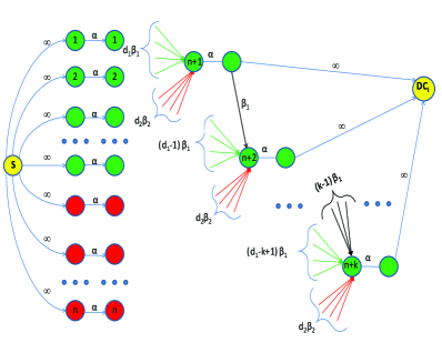
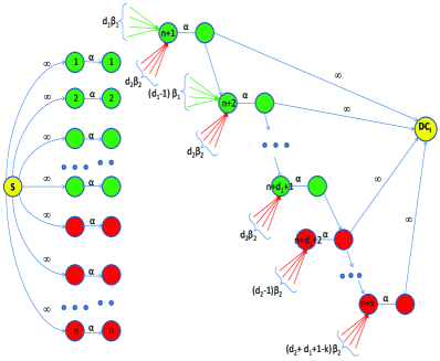
Figure 2: General information flow graphs corresponding to the cases $k\leq d_{c}+1$ (left) and $k>d_{c}+1$ (right).

II-B2 Case $k>d_{c}+1$

This case corresponds to the situation when the data collector connects to $d_{c}+1$ replaced nodes from the set $V^{1}$ and to $k-d_{c}-1$ replaced nodes from the set $V^{2}$. With this scenario shown in the information flow graph of Figure 2 right, the mincut analysis leads to

$$\sum_{i=0}^{d_{c}}\min({d_{c}\beta_{c}+d_{e}\beta_{e}-i\beta_{c},\alpha})+\sum_{i=d_{c}+1}^{k-1}\min({(d_{c}+d_{e}-i)\beta_{e},\alpha})\geq M.$$ (4)

After applying $\beta_{c}=\tau\beta_{e}$ and an optimization process, the mincut equation (4) leads to the following threshold function:

$$\alpha^{*}(d_{c},d_{e},\beta_{e})=\left\{\begin{array}[]{ll}\frac{M}{k},&\beta_{e}\in[f_{1}(0),+\infty)\\ \\ \frac{2M-g(i)\beta_{e}}{2(k-i)},&\beta_{e}\in[f_{1}(i),f_{1}(i-1))\\ &i=1,\ldots,k-d_{c}-1\\ \\ \frac{2M-(g_{1}(i)(k-d_{c}-1)g_{2}(i))\beta_{e}}{2(d_{c}-i)},&\beta_{e}\in[f_{2}(i),f_{2}(i-1)),\\ &i=k-d_{c},\ldots,k-1,\end{array}\right.$$ (5)

where

$$f_{1}(i)=\frac{2M}{2k(d-k)+(i+1)+(2k-1)},$$

$$f_{2}(i)=\frac{2M}{(2kd-k^{2}-d_{c}^{2}-d_{c}+k+2d_{c}\tau)+i\tau(2d_{c}-i-1)},$$

$$g_{1}(i)=i(2d-2k+i+1),\text{ and}$$

$$g_{2}(i)=(i+1)(2d_{e}+i\tau).$$

III Two-rack model

In this model, the cost of sending data to a newcomer in a different rack is higher than the cost of sending data to a newcomer in the same rack. Note the difference of this rack model compared with the static cost model described in Subsection II-B. In that model, there is a static classification of the storage nodes between the ones having “cheap bandwidth” and the ones having “expensive bandwidth”. In our new model, this classification depends on each newcomer. When a storage node fails and a newcomer enters into the system, nodes from the same rack are in the “cheap bandwidth” set, while nodes in other racks are in the “expensive bandwidth” set. In this section, we analyze the case when there are only two racks. Let $V_{1}$ and $V_{2}$ be the sets of $n_{1}$ and $n_{2}$ storage nodes from the first and second rack, respectively.

Consider the same situation as in Subsection II-B, but now the sets of “cheap bandwidth” and “expensive bandwidth” nodes depend on the specific replaced node. Again, we can assume, without loss of generality, that $\beta_{c}=\tau\beta_{e}$ for some real number $\tau\geq 1$. Let the newcomers be the storage nodes $s_{j}$, $j=n+1,\ldots,\infty$. Let $d=d_{c}^{1}+d_{e}^{1}=d_{c}^{2}+d_{e}^{2}$ be the number of helper nodes for any newcomer, where $d_{c}^{1}$, $d_{e}^{1}$ and $d_{c}^{2}$, $d_{e}^{2}$ are the number of cheap and expensive bandwidth helper nodes of a newcomer in the first and second rack, respectively. We can always assume that $d_{c}^{1}\leq d_{c}^{2}$, by swapping racks if it is necessary.

In the model described in Subsection II-A, the repair bandwidth $\gamma$ is the same for any newcomer. In the rack model, it depends on the rack where the newcomer is placed. Let $\gamma^{1}=\beta_{e}(d_{c}^{1}\tau+d_{e}^{1})$ be the repair bandwidth for any newcomer in the first rack with repair cost $C_{T}^{1}=\beta_{e}(C_{c}d_{c}^{1}\tau+C_{e}d_{e}^{1})$, and let $\gamma^{2}=\beta_{e}(d_{c}^{2}\tau+d_{e}^{2})$ be the repair bandwidth for any newcomer in the second rack with repair cost $C_{T}^{2}=\beta_{e}(C_{c}d_{c}^{2}\tau+C_{e}d_{e}^{2})$. Note that if $d_{c}^{1}=d_{c}^{2}$ or $\tau=1$, then $\gamma^{1}=\gamma^{2}$, otherwise $\gamma^{1}<\gamma^{2}$. As it is mentioned in [3], in order to represent a distributed storage system, the information flow graph is restricted to $\gamma\geq\alpha$. In the rack model, it is necessary that $\gamma^{1}\geq\alpha$, which means that $\gamma^{2}\geq\alpha$.

Moreover, unlike the models described in Section II, where it is straightforward to establish which is the set of nodes which minimize the mincut, in the rack model, this set of nodes may change depending on the parameters $k$, $d_{c}^{1}$, $d_{c}^{2}$, $n_{1}$ and $\tau$. We call to this set of newcomers, the minimum mincut set. Recall that the income of a newcomer $s_{j}$, $j=n+1,\ldots,\infty$, is the sum of the weights of the arcs that should be cut in order to isolate $v_{in}^{j}$ from $S$. Let $I$ be the indexed multiset containing the incomes of $k$ newcomers which minimize the mincut. It is easy to see that in the model described in Subsection II-A, $I=\{(d-i)\beta\;|\;i=0,\ldots,k-1\}$, and in the one described in Subsection II-B, $I=\{((d_{c}-i)\tau+d_{e})\beta_{e}\;|\;i=0,\ldots,\min(d_{c},k-1)\}\cup\{(d_{e}-i)\beta_{e}\;|\;i=1,\ldots,k-d_{c}-1\}$. Note that when $k\leq d_{c}+1$, $\{(d_{e}-i)\beta_{e}\;|\;i=1,\ldots,k-d_{c}-1\}$ is empty.

In order to establish $I$ in the rack model, the set of $k$ newcomers which minimize the mincut must be found. First, note that since $d_{c}^{1}\leq d_{c}^{2}$, the income of the newcomers is minimized by replacing first $d_{c}^{1}+1$ nodes from the rack with less number of helper nodes, which in fact minimizes the mincut. Therefore, the indexed multiset $I$ always contains the incomes of a set of $d_{c}^{1}+1$ newcomers from $V_{1}$. Define $I_{1}=\{((d_{c}^{1}-i)\tau+d_{e}^{1})\beta_{e}\;|\;i=0,\ldots,\min(d_{c}^{1},k-1)\}$ as the indexed multiset where $I_{1}[i]$, $i=0,\ldots,\min(d_{c}^{1},k-1)$, are the incomes of this set of $d_{c}^{1}+1$ newcomers from $V^{1}$. If $k\leq d_{c}^{1}+1$, then $I=I_{1}$, otherwise $I_{1}\subset I$ and $k-d_{c}^{1}-1$ more newcomers which minimize the mincut must be found.

When $k>d_{c}^{1}+1$, we will see that there are two possibilities, either the remaining nodes from $V_{1}$ are in the set of newcomers which minimize the mincut or not. Define $I_{2}=\{d_{e}^{1}\beta_{e}\;|\;i=1,\ldots,\min(k-d_{c}^{1}-1,n_{1}-d_{c}^{1}-1)\}\cup\{(d_{c}^{2}-i)\tau\beta_{e}\;|\;i=0,\ldots,\min(d_{c}^{2},k-n_{1}-1)\}$ as the indexed multiset where $I_{2}[i]$, $i=0,\ldots,k-d_{c}^{1}-2$, are the incomes of a set of $k-d_{c}^{1}-1$ newcomers, including the remaining $n_{1}-d_{c}^{1}-1$ newcomers from $V_{1}$ and newcomers from $V_{2}$. Note that if $n_{1}-d_{c}^{1}-1>k-d_{c}^{1}-1$, it only contains newcomers from $V_{1}$. Define $I_{3}=\{(d_{c}^{2}-i)\tau\beta_{e}\;|\;i=0,\ldots,\min(d_{c}^{2},k-d_{c}^{1}-2)\}$ as the indexed multiset where $I_{3}[i]$, $i=0,\ldots,k-d_{c}^{1}-2$, are the incomes of a set of $k-d_{c}^{1}-1$ newcomers from $V_{2}$. When $d_{c}^{2}<k-d_{c}^{1}-1$ or $d_{c}^{2}<k-n_{1}$, according to the information flow graph, the remaining incomes necessary to complete the set of $k-d_{c}^{1}-1$ newcomers are zero. Therefore, it can be assumed that $d_{c}^{2}\geq k-d_{c}^{1}-1\geq k-n_{1}$, since the mincut equation does not change when $d_{c}^{2}<k-d_{c}^{1}-1$ or $d_{c}^{2}<k-n_{1}$.

Proposition 1.

If $k>d_{c}^{1}+1$, we have that $|I_{2}|=|I_{3}|=k-d_{c}^{1}-1$. Moreover, if $\sum_{i=0}^{k-d_{c}^{1}-2}I_{2}[i]<\sum_{i=0}^{k-d_{c}^{1}-2}I_{3}[i]$, then $I=I_{1}\cup I_{2}$; otherwise $I=I_{1}\cup I_{3}$.

Proof:    We need to prove that $I_{2}$ and $I_{3}$ are the only possible sets of incomes which minimize the mincut. We will see that it is not possible to find a set of incomes such that the sum of all its elements is less than $\min(\sum_{i=0}^{|I_{2}|-1}I_{2}[i],\sum_{i=0}^{|I_{3}|-1}I_{3}[i])$.

Let $A=I_{2}-(I_{2}\cap I_{3})=\{a_{1},a_{2},\ldots,a_{n}\;|\;a_{i}=a_{j},i<j\}$ and $B=I_{3}-(I_{2}\cap I_{3})=\{b_{1},b_{2},\ldots,b_{n}\;|\;b_{i}>b_{j},i<j\}$. Let $D=A\cup B=\{d_{1},d_{2},\ldots,d_{2n}\;|\;d_{i}\geq d_{j},i<j\}$. Then, $\sum_{i=1}^{n}d_{i}\geq\sum_{i=1}^{n}b_{i}$ and $\sum_{i=1}^{n}d_{i}\geq\sum_{i=1}^{n}a_{i}$. Note that $A$, $B$ and $D$ are incomes of an information flow graph, which means that one can not add $d_{2}$ without having added $d_{1}$ to the sum. The same happens with $A$ or $B$, so the elements must be included in order from the highest to the lowest. ∎

If $k\leq d_{c}^{1}+1$, $I=I_{1}$ and the corresponding mincut equation is

$$\sum_{i=0}^{|I_{1}|-1}\min(I_{1}[i],\alpha)\geq M.$$ (6)

On the other hand, if $k>d_{c}^{1}+1$ and $I=I_{1}\cup I_{2}$, the corresponding mincut equation is

$$\sum_{i=0}^{|I_{1}|-1}\min(I_{1}[i],\alpha)+\sum_{i=0}^{|I_{2}|-1}\min(I_{2}[i],\alpha)\geq M,$$ (7)

and if $I=I_{1}\cup I_{3}$, the equation is

$$\sum_{i=0}^{|I_{1}|-1}\min(I_{1}[i],\alpha)+\sum_{i=0}^{|I_{3}|-1}\min(I_{3}[i],\alpha)\geq M.$$ (8)

In the previous models described in Section II, the decreasing behavior of the incomes included in the mincut equation is used to find the threshold function which minimizes the parameters $\alpha$ and $\gamma$. In the rack model, the incomes included in the mincut equations may not have a decreasing behavior as the newcomers enter into the system, so it is necessary to find the threshold function in a different way.

Let $L$ be the increasing ordered list of values such that for all $i,\;i=0,\ldots,k-1$, $I[i]/\beta_{e}\in L$ and $|I|=|L|$. Note that any of the information flow graphs, which represent the rack model or any of the two models from Section II, can be described in terms of $I$, so they can be represented by $L$. Therefore, once $L$ is found, it is possible to find the parameters $\alpha$ and $\beta_{e}$ (and then $\gamma$ or $\gamma^{1}$ and $\gamma^{2}$) using the threshold function given in the next theorem. Note that the way to represent this threshold function for the rack model can be seen as a generalization, since it also represents the behavior of the mincut equations for the previous given models.

Theorem 1.

The threshold function $\alpha^{*}(\beta_{e})$ (which also depends on $d$, $d_{c}^{1}$, $d_{c}^{2}$, $k$ and $\tau$) is the following:

$$\alpha^{*}(\beta_{e})=\left\{\begin{array}[]{ll}\frac{M}{k},&\beta_{e}\in[f(0),+\infty)\\ &\\ \frac{M-g(i)\beta_{e}}{k-i},&\beta_{e}\in[f(i),f(i-1))\\ &i=1,\ldots,k-1,\end{array}\right.$$ (9)

subject to $\gamma^{1}=(d_{c}^{1}\tau+d_{e}^{1})\beta_{e}\geq\alpha$, where

$$f(i)=\frac{M}{L[i](k-i)+g(i)}\;\text{ and }\;g(i)=\sum_{j=0}^{i-1}L[j].$$

Note that $f(i)$ is a decreasing function and $g(i)$ is an increasing function.

Proof:    We want to obtain the threshold function which minimizes $\alpha$, that is,

$$\begin{array}[]{ll}\alpha^{*}(\beta_{e})=&\min\alpha\\ &\text{subject to: }\sum_{i=0}^{k-1}\min(L[i]\beta_{e},\alpha)\geq M.\end{array}$$ (10)

Therefore, we are going to show the optimization of (10) which leads to the threshold function (9).

Define $M^{*}$ as

$$M^{*}=\sum_{i=0}^{k-1}\min(L[i]\beta_{e},\alpha).$$

Note that $M^{*}$ is a piecewise linear function of $\alpha$. Since $L$ is a sorted list of $k$ values, if $\alpha$ is less than the lowest value $L[0]$, then $M^{*}=k\alpha$. As $\alpha$ grows, the values from $L$ are added to the equation, so

$$M^{*}=\left\{\begin{array}[]{ll}k\alpha,&\alpha\in[0,L[0]\beta_{e}]\\ \\ (k-i)\alpha+\sum_{j=0}^{i-1}L[j]\beta_{e},&\alpha\in(L[i-1]\beta_{e},L[i]\beta_{e}]\\ &i=1,\ldots,k-1\\ \\ \sum_{j=0}^{k-1}L[j]\beta_{e},&\alpha\in(L[k-1]\beta_{e},\infty).\end{array}\right.$$ (11)

Using that $M^{*}\geq M$, we can minimize $\alpha$ depending on $M$. Note that the term $\sum_{j=0}^{k-1}L[j]\beta_{e}$ of the previous equation has no significance in the minimization of $\alpha$, so it can be ignored. Therefore, we obtain the function

$$\alpha^{*}=\left\{\begin{array}[]{ll}\frac{M}{k},&M\in[0,kL[0]\beta_{e}]\\ \\ \frac{M-\sum_{j=0}^{i-1}L[j]\beta_{e}}{k-i},&M\in(L[i-1]\beta_{e}(k-i)+\sum_{j=0}^{i-1}L[j]\beta_{e},\\ &L[i]\beta_{e}(k-i)+\sum_{j=0}^{i-1}L[j]\beta_{e}]\\ &i=1,\ldots,k-1.\end{array}\right.$$ (12)

Finally, define $g(i)=\sum_{j=0}^{i-1}L[j]$ and $f(i)=\frac{M}{L[i](k-i)+g(i)}$. Then, the above expression of $\alpha^{*}$ can be defined over $\beta_{e}$ instead of over $M$, and the threshold function (9) follows. ∎

Figure 3: Information flow graph corresponding to the rack model when $k>d_{c}^{1}+1$, with $k=4$, $d_{c}^{1}=1$, $d_{c}^{2}=2$, $d=4$ and $n_{1}=n_{2}=3$.

Example III.1.

Figure 3 shows the example of an information flow graph corresponding to a regenerating code with $k=4$, $d_{c}^{1}=1$, $d_{c}^{2}=2$, $d=4$ and $n_{1}=n_{2}=3$. Taking for example $\tau=2$, we have that $I_{1}=\{5\beta_{e},3\beta_{e}\}$, $I_{2}=\{3\beta_{e},4\beta_{e}\}$ and $I_{3}=\{4\beta_{e},2\beta_{e}\}$. By Proposition 1, since $\sum_{i=0}^{1}I_{2}[i]>\sum_{i=0}^{1}I_{3}[i]$, $I=I_{1}\cup I_{3}=\{5\beta_{e},3\beta_{e},4\beta_{e},2\beta_{e}\}$, and then $L=[2,3,4,5]$. The corresponding mincut equation is (8) and applying $L$ to the threshold function (9), we obtain

$$\alpha^{*}(\beta_{e})=\left\{\begin{array}[]{ll}\frac{M}{4},&\beta_{e}\in[\frac{M}{8},+\infty)\\ &\\ \frac{M-2\beta_{e}}{3},&\beta_{e}\in[\frac{M}{11},\frac{M}{8})\\ &\\ \frac{M-5\beta_{e}}{2},&\beta_{e}\in[\frac{M}{13},\frac{M}{11})\\ &\\ M-9\beta_{e},&\beta_{e}\in[\frac{M}{14},\frac{M}{13}).\\ \end{array}\right.$$ (13)

It can happen that two consecutive values in $L$ are equal, that is $L[i]=L[i-1]$, so $f(i)=f(i-1)$. In this case, we consider that the interval $[f(i),f(i-1))$ is empty and it can be deleted.

Example III.2.

Figure 4 shows the same example as Figure 3 with an information flow graph corresponding to a regenerating code with $d_{c}^{1}=1$, $d_{c}^{2}=2$, $d=4$ and $n_{1}=n_{2}=3$, but taking $k=3$ instead of $k=4$. If for example $\tau=2$, we have that $I_{1}=\{5\beta_{e},3\beta_{e}\}$, $I_{2}=\{3\beta_{e}\}$ and $I_{3}=\{4\beta_{e}\}$. By Proposition 1, since $\sum_{i=0}^{0}I_{2}[i]<\sum_{i=0}^{0}I_{3}[i]$, $I=I_{1}\cup I_{2}=\{5\beta_{e},3\beta_{e},3\beta_{e}\}$, and then $L=[3,3,5]$. The corresponding mincut equation is (7) and applying $L$ to the threshold function (9), we obtain

$$\alpha^{*}(\beta_{e})=\left\{\begin{array}[]{ll}\frac{M}{3},&\beta_{e}\in[\frac{M}{9},+\infty)\\ \\ \frac{M-3\beta_{e}}{2},&\beta_{e}\in[\frac{M}{9},\frac{M}{9})\\ \\ M-6\beta_{e},&\beta_{e}\in[\frac{M}{11},\frac{M}{9}).\end{array}\right.$$ (14)

Note that the second interval is empty and it can be deleted.

Figure 4: Information flow graph corresponding to the rack model when $k>d_{c}^{1}+1$, with $k=3$, $d_{c}^{1}=1$, $d_{c}^{2}=2$, $d=4$ and $n_{1}=n_{2}=3$.

Finally, note that when $k\leq d_{c}^{1}+1$, the mincut equations and the threshold function (9) for the rack model are exactly the same as the ones shown in [5] for the model described in Subsection II-B. Actually, it can be seen that $d_{c}^{1}$ of the rack model is equivalent to $d_{c}$ of the static cost model. Indeed, it can be seen that when $k\leq d_{c}^{1}+1$, the rack model and the static cost model have the same behavior because $I=I_{1}$.

III-A MSR and MBR points

The threshold function (9) leads to a tradeoff curve between $\alpha$ and $\beta_{e}$. Note that, like in the static cost model, since there is a different repair bandwidth $\gamma^{1}$ and $\gamma^{2}$ for each rack, this curve is based on $\beta_{e}$ instead of $\gamma^{1}$ and $\gamma^{2}$.

At the MSR point, the amount of stored data per node is $\alpha_{MSR}=M/k$. Moreover, at this point, the minimum value of $\beta_{e}$ is $\beta_{e}=f(0)=\frac{M}{L[0]k}$, which leads to

$$\gamma^{1}_{MSR}=\frac{(d_{c}^{1}\tau+d_{e}^{1})M}{L[0]k}\quad\textrm{and}\quad\gamma^{2}_{MSR}=\frac{(d_{c}^{2}\tau+d_{e}^{2})M}{L[0]k}.$$

On the other hand, at the MBR point, as $f(i)$ is a decreasing function, the parameter $\beta_{e}$ which leads to the minimum repair bandwidths is $\beta_{e}=f(|L|-1)=\frac{M}{L[|L|-1](k-|L|+1)+g(|L|-1)}$. Then, the corresponding amount of stored data per node is $\alpha_{MBR}=\frac{ML[|L|-1]}{(k-|L|+1)L[|L|-1]+g(|L|-1)}$, and the repair bandwidths are

$$\gamma^{1}_{MBR}=\frac{(d_{c}^{1}\tau+d_{e}^{1})M}{L[|L|-1](k-|L|+1)+g(|L|-1)}\quad\textrm{and}$$

$$\gamma^{2}_{MBR}=\frac{(d_{c}^{2}\tau+d_{e}^{2})M}{L[|L|-1](k-|L|+1)+g(|L|-1)}.$$

III-B Non-feasible situation

As we have seen, the threshold function (9) is subject to $\gamma^{1}=(d_{c}^{1}\tau+d_{e}^{1})\beta_{e}\geq\alpha$.

Proposition 2.

If the inequality $\gamma^{1}\geq\alpha$ is achieved, then $\max(L)=I_{1}[0]/\beta_{e}$.

Proof:    Since $L$ is an increasing ordered list, for $i=0,\ldots,k-1$, $\max(L)=L[k-1]$. As $I_{1}[0]$ is the income of the first newcomer, then $I_{1}[0]/\beta_{e}=d_{c}^{1}\tau+d_{e}^{1}\in L$. Actually, $L$ is constructed from all elements in $I$ and $I_{1}\subseteq I$, by Proposition 1.

If $\gamma^{1}\geq\alpha$, then taking $\beta_{e}=f(k-1)$ in Theorem 1, we have that $\gamma^{1}=(d_{c}^{1}\tau+d_{e}^{1})\beta_{e}=(d_{c}^{1}\tau+d_{e}^{1})f(k-1)\geq M-g(k-1)f(k-1)$. After some operations, we obtain that $\frac{(d_{c}^{1}\tau+d_{e}^{1})M}{\sum_{j=0}^{k-1}L[j]}\geq\frac{L[k-1]M}{\sum_{j=0}^{k-1}L[j]}$, so $d_{c}^{1}\tau+d_{e}^{1}\geq L[k-1]$. Since $I_{1}[0]/\beta_{e}=d_{c}^{1}\tau+d_{e}^{1}\in L$ and $\max(L)=L[k-1]$, $d_{c}^{1}\tau+d_{e}^{1}=L[k-1]=I_{1}[0]/\beta_{e}$. ∎

Since any distributed storage system satisfies that $\gamma^{1}\geq\alpha$, we have that $\max(L)=I_{1}[0]/\beta_{e}$, by Proposition 2. In order to have this situation, we need to remove from $L$ any value $L[i]$ such that $L[i]>I_{1}[0]/\beta_{e}$, $i=0,\ldots,k-1$. After that, we can assume that $L[|L|-1]=I_{1}[0]/\beta_{e}$. In terms of the tradeoff curve, this means that there is no point in the curve that outperforms the MBR point.

Example III.3.

In order to illustrate this situation, we can consider the example of a regenerating code with $k=3$, $d_{c}^{1}=1$, $d_{c}^{2}=4$, $d=6$, $n_{1}=2$ and $n_{2}=5$, and the information flow graph given in Figure 5. Taking $\tau=2$, the incomes of the newcomers $s_{n+1}$, $s_{n+2}$ and $s_{n+3}$ are $7\beta_{e}$, $5\beta_{e}$ and $8\beta_{e}$, respectively. Actually, we have that $I=I_{1}\cup I_{2}$, where $I_{1}=\{7\beta_{e},5\beta_{e}\}$ and $I_{2}=\{8\beta_{e}\}$. Then, $L=[5,7,8]$, so $\max{(L)}=8>I[0]/\beta_{e}=7$. Applying $L$ to the threshold function (9), the resulting minimization of $\alpha$ and $\beta_{e}$ is

$$\alpha^{*}(\beta_{e})=\left\{\begin{array}[]{ll}\frac{M}{3},&\beta_{e}\in[\frac{M}{15},+\infty)\\ \\ \frac{M-5\beta_{e}}{2},&\beta_{e}\in[\frac{M}{19},\frac{M}{15})\\ \\ M-12\beta_{e},&\beta_{e}\in[\frac{M}{20},\frac{M}{19}).\end{array}\right.$$

Note that considering the last interval, we have that for $\beta_{e}=f(k-1)=\frac{M}{20}$, $\alpha_{MBR}=\frac{8M}{20}$ and $\gamma^{1}_{MBR}=(d_{c}^{1}\tau+d_{e}^{1})f(k-1)=\frac{7M}{20}$. Applied to the information flow graph, we obtain that $\mbox{mincut}(S,DC)=\frac{7M}{20}+\frac{5M}{20}+\frac{8M}{20}=M$ which is true. However, since $\alpha_{MBR}>\gamma^{1}_{MBR}$, it gives a non-feasible situation for a distributed storage scheme. Note also that if we delete this non-feasible interval, then $\gamma^{1}_{MBR}=\frac{7M}{19}$ and $\alpha_{MBR}=\frac{7M}{19}$ which corresponds to the MBR point because $\gamma^{1}_{MBR}=\alpha_{MBR}$.

It is important to note that more than one element from $I$ can be greater than any element from $I_{1}$, which will result in more impossible intervals. In conclusion, any value from $I$ greater than the greatest value from $I_{1}$, must be deleted because otherwise it would lead to a non-feasible situation.

Figure 5: Information flow graph with $k=3$, $n_{1}=2$, $n_{2}=5$, $d_{c}^{1}=1$, $d_{c}^{2}=4$ and $d=6$.

III-C Case $d_{e}^{1}\beta_{e}\geq d_{c}^{2}\tau\beta_{e}$

In this case, the mincut equation has a decreasing behavior as $i$ increases for $i=0,\ldots,k-1$. Therefore, it is possible to define an injective function with a decreasing behavior, which will be used to determine the intervals of the threshold function. Basically, it is possible to use the same procedure shown in [3] and [5] to find the threshold function. Moreover, it can be seen that the set of incomes which minimize the mincut is always the same, it does not depend on any parameter.

It is easy to see that if $d_{e}^{1}\beta_{e}\geq d_{c}^{2}\tau\beta_{e}$ and $k\leq d_{c}^{1}+1$, the mincut equations (and so the threshold functions) corresponding to the model explained in this section and the model explained in Subsection II-B are exactly the same. Therefore, we will focus on the situation that $d_{e}^{1}\beta_{e}\geq d_{c}^{2}\tau\beta_{e}$ and $k>d_{c}^{1}+1$. Note that this is in fact a particular case of the general threshold function (9), where it is possible to create a decreasing function for any feasible $i$, and then find the threshold function giving more details.

Theorem 2.

When $d_{e}^{1}\geq d_{c}^{2}\tau$ and $k>d_{c}^{1}+1$, the threshold function $\alpha^{*}(\beta_{e})$ (which also depends on $d$, $d_{c}^{1}$, $d_{c}^{2}$, $k$ and $\tau$) is the following:

$$\alpha^{*}(\beta_{e})=\left\{\begin{array}[]{ll}\frac{M}{k},&\beta_{e}\in[f_{1}(0),+\infty)\\ \\ \frac{M-g_{1}(i)\tau\beta_{e}}{k-i},&\beta_{e}\in[f_{1}(i),f_{1}(i-1))\\ &i=1,\ldots,k-d_{c}^{1}-2\\ \\ \frac{M-g_{1}(k-d_{c}^{1}-1)\tau\beta_{e}}{k-i},&\beta_{e}\in[f_{2}(k-d_{c}^{1}-1),f_{1}(k-d_{c}^{1}-2))\\ \\ \frac{M-g_{1}(k-d_{c}^{1}-1)\tau\beta_{e}-g_{2}(i-k+d_{c}^{1}+1)\beta_{e}}{k-i},&\beta_{e}\in[f_{2}(i),f_{2}(i-1))\\ &i=k-d_{c}^{1},\ldots,k-1,\end{array}\right.$$ (15)

where

$$g_{1}(i)=\frac{i}{2}(2d-2k+i+1),$$

$$g_{2}(i)=\frac{i}{2}(2d_{e}^{1}+\tau i-\tau),$$

$$f_{1}(i)=\frac{2M}{\tau(2k(d-k)+(i+1)(2k-i))},\text{ and }$$

$$f_{2}(i)=\frac{2M}{2d_{e}^{1}+2d_{e}^{1}d_{c}^{1}-\tau(i(i-2k+1)+2(k^{2}-k-kd+d_{e}^{1}+d_{e}^{1}d_{c}^{1}))}.$$

Note that $f_{1}(i)$ and $f_{2}(i)$, $i=0,\ldots,k-1$, are decreasing functions, and $g_{1}(i)$ and $g_{2}(i)$, $i=1,\ldots,k-1$, are increasing functions.

Proof:    Note that $d_{e}^{1}=d_{c}^{2}+1$ and $d_{e}^{2}=d_{c}^{1}+1$. We consider the mincut equation (8) of the rack model, since if $d_{e}^{1}\geq d_{c}^{2}\tau$, then we have that $I=I_{1}\cup I_{3}$, by Proposition 1. In other words, the $n_{1}-d_{c}^{1}-1$ remaining newcomers from $V^{1}$ are not in the set of newcomers which minimizes the mincut. Assume that $k\leq d=d_{c}^{1}+d_{e}^{1}$ because if $d<k$, requiring any $d$ storage nodes to have a flow of $M$ will lead to the same condition as requiring any $k$ storage nodes to have a flow of $M$ [3]. We want to obtain the threshold function which minimizes $\alpha$, that is,

$$\begin{array}[]{ll}\alpha^{*}(\beta_{e})=&\min\alpha\\ &\text{subject to: }\sum_{i=0}^{d_{c}^{1}}\min(d_{c}^{1}\beta_{c}+d_{e}^{1}\beta_{e}-i\beta_{c},\alpha)+\\ &\sum_{i=d_{c}^{1}+1}^{k-1}\min((d_{c}^{1}+d_{e}^{1}-i)\beta_{c},\alpha)\geq M.\end{array}$$ (16)

Therefore, we are going to show the optimization of (16) which leads to (15).

Applying that $\beta_{c}=\tau\beta_{e}$, we can define the minimum $M$ as $M^{*}$, so

$$M^{*}=\sum_{i=0}^{d_{c}^{1}}\min((d_{c}^{1}\tau+d_{e}^{1}-i\tau)\beta_{e},\alpha)+\sum_{i=d_{c}^{1}+1}^{k-1}\min((d_{c}^{1}+d_{e}^{1}-i)\tau\beta_{e},\alpha).$$

In order to change the order of the above summation, we define

$$b(i_{1},i_{2})=d_{c}^{1}+d_{e}^{1}-k+1+i_{1}+i_{2}\tau.$$

Note that $M^{*}$ is a piecewise linear function of $\alpha$. The minimum value of $\{(d_{c}^{1}\tau+d_{e}^{1}-i\tau)\beta_{e}\;|\;i=0,\ldots,d_{c}^{1}\}\cup\{(d_{c}^{1}+d_{e}^{1}-i)\tau\beta_{e}\;|\;i=d_{c}^{1}+1,\ldots,k-1\}$ is when $i=k-1$. Therefore, if $\alpha$ is less than this value, then $M^{*}=k\alpha$. Since $d_{e}^{1}=d_{c}^{2}+1$ and $d_{e}^{2}=d_{c}^{1}+1$ the lowest value of $\{(d_{c}^{1}\tau+d_{e}^{1}-i\tau)\beta_{e}\;|\;i=0,\ldots,d_{c}^{1}\}$ which is $d_{e}^{1}\beta_{e}$, is higher than or equal to the highest value of $\{(d_{c}^{1}+d_{e}^{1}-i)\tau\beta_{e}\;|\;i=d_{c}^{1}+1,\ldots,k-1\}$, which is $(d_{e}^{1}-1)\tau\beta_{e}$. This means that as $\alpha$ increases, the term $(d_{c}^{1}+d_{e}^{1}-i)\tau\beta_{e}$ is added more times in $M^{*}$ while $i=k-1,\ldots,d_{c}^{1}$. When $i=d_{c}^{1},\ldots,0$, the term $(d_{c}^{1}\tau+d_{e}^{1}-i\tau)\beta_{e}$ is added more times in $M^{*}$.

$$M^{*}=\left\{\begin{array}[]{ll}k\alpha,&\alpha\in[0,b(0,0)\tau\beta_{e}]\\ &\\ \\ (k-i)\alpha+\sum_{j=0}^{i-1}b(j,0)\tau\beta_{e},&\alpha\in(b(i-1,0)\tau\beta_{e},b(i,0)\tau\beta_{e}]\\ &i=1,\ldots,k-d_{c}^{1}-2\\ \\ (d_{c}^{1}+1)\alpha+\sum_{j=0}^{k-d_{c}^{1}-2}b(j,0)\tau\beta_{e},&\alpha\in(b(k-d_{c}^{1}-2,0)\tau\beta_{e},\\ &b(k-d_{c}^{1}-1,0)\beta_{e}]\\ &\\ \\ (k-i)\alpha+\sum_{j=0}^{k-d_{c}^{1}-2}b(j,0)\tau\beta_{e}+\\ \sum_{j=0}^{i-k+d_{c}^{1}}b(k-d_{c}^{1}-1,j)\beta_{e},&\alpha\in(b(k-d_{c}^{1}-1,i-k+d_{c}^{1})\beta_{e},\\ &b(k-d_{c}^{1}-1,i-k+d_{c}^{1}+1)\beta_{e}]\\ &i=k-d_{c}^{1},\ldots,k-1\\ \sum_{j=0}^{k-d_{c}^{1}-2}b(j,0)\tau\beta_{e}+\\ \sum_{j=0}^{d_{c}^{1}}b(k-d_{c}^{1}-1,j)\beta_{e},&\alpha\in(b(k-d_{c}^{1}-1,d_{c}^{1})\beta_{e},\infty).\\ &\end{array}\right.$$ (17)

Using that $M\geq M^{*}$, we can minimize $\alpha$ depending on $M$. Note that the last term of (17) does not affect in the minimization of $\alpha$, so it is ignored. Therefore, we obtain the function

$$\alpha^{*}=\left\{\begin{array}[]{ll}\frac{M}{k},&M\in[0,kb(0,0)\tau\beta_{e}]\\ \\ \frac{M-\sum_{j=0}^{i-1}b(j,0)\tau\beta_{e}}{k-i},&M\in(A(i-1),A(i)]\\ &i=1,\ldots,k-d_{c}^{1}-2\\ \frac{M-\sum_{j=0}^{i-1}b(j,0)\tau\beta_{e}}{k-i},&M\in(A(i-1),B(i)]\\ \\ \frac{M-\sum_{j=0}^{k-d_{c}^{1}-2}b(j,0)\tau\beta_{e}-\sum_{j=0}^{i-k+d_{c}^{1}}b(k-d_{c}^{1}-1,j)\beta_{e}}{k-i},&M\in(B(i-1),B(i)]\\ &i=k-d_{c}^{1},\ldots,k-1,\end{array}\right.$$ (18)

where $A(i)=\tau\beta_{e}(b(i,0)(k-i-1)+\sum_{j=0}^{i}b(j,0))$ and $B(i)=\beta_{e}(b(k-d_{c}^{1}-1,i-k+d_{c}^{1}+1)(k-i-1)+\sum_{j=0}^{k-d_{c}^{1}-2}b(j,0)\tau+\sum_{j=0}^{i-k+d_{c}^{1}+1}b(k-d_{c}^{1}-1,j))$.

From the definition of $b(i_{1},i_{2})$,

$$\sum_{j=0}^{i-1}b(j,0)=\frac{i}{2}(2d-2k+i+1)=g_{1}(i),$$

$$\sum_{j=0}^{i-1}b(k-d_{c}^{1}-1,j)=\frac{i}{2}(2d_{e}^{1}+\tau i-\tau)=g_{2}(i),$$

$$\tau((k-i-1)b(i,0)+\sum_{j=0}^{i}b(j,0))=\frac{2M}{\tau(2k(d-k)+(i+1)(2k-i))}=\frac{M}{f_{1}(i)}$$

and

$$b(k-d_{c}^{1}-1,i-k+d_{c}^{1}+1)(k-i-1)+\sum_{j=0}^{k-d_{c}^{1}-2}b(j,0)\tau+\sum_{j=0}^{i-k+d_{c}^{1}+1}b(k-d_{c}^{1}-1,j)=\frac{M}{f_{2}(i)}.$$

The function (18) for $\alpha^{*}$ can be defined over $\beta_{e}$ instead of over $M$, and then function (15) follows. ∎

IV General rack model

Let $r\geq 2$ be the number of racks of a distributed storage system. Let $n_{j}$, $j=1,\ldots,r$, be the number of storage nodes in the $j$-th rack. Let $d_{c}^{j}$ be the number of helper nodes providing cheap bandwidth and $d_{e}^{j}$ be the number of helper nodes providing expensive bandwidth to any newcomer in the $j$-th rack. We assume that the total number of helper nodes $d$ is fixed, so it is satisfied that $d=d_{c}^{j}+d_{e}^{j}$ for $j=1,\ldots,r$. Moreover, it can be seen that $d_{e}^{j}=\sum_{z=1,z\neq j}^{r}(d_{c}^{z}+1)$. Let the racks be increasingly ordered by number of cheap bandwidth nodes, so $i\leq j$ if and only if $d_{c}^{i}\leq d_{c}^{j}$. First, we consider the case when $d=n-1$, and then the general case, that is, when $d\leq n-1$

IV-A When $d=n-1$

In this case, we impose that any available node in the system is a helper node, that is, $d=n-1$. If one node fails in the $j$-th rack, $d_{c}^{j}=n_{j}-1$ nodes from the same rack and $d_{e}^{j}=n-n_{j}$ nodes from other racks help in the regeneration process.

The indexed multiset $I$ containing the incomes of the $k$ newcomers which minimize the mincut is

$$I=\bigcup_{j=1}^{r}\{((d_{c}^{j}-i)\tau+d_{e}^{j}-\sum_{z=1}^{j-1}(d_{c}^{z}-j+1)\beta_{e}\;|\;i=0,\ldots,\min(d_{c}^{j},k-\sum_{z=1}^{j-1}d_{c}^{z}-j)\},$$ (19)

where $\sum_{z=1}^{0}x=0$ for any value $x$. Therefore, the resulting mincut equation is $\sum_{i=0}^{k-1}\min(I[i],\alpha)\geq M$.

Finally, the threshold function (9) can be applied, so $\alpha$ and $\beta_{e}$ can be minimized. Note that the set of $k$ newcomers which minimize the mincut is fixed independently of $\tau$, so there is only one candidate set to be the minimum mincut set.

IV-B When $d\leq n-1$

In this case, there may exist nodes in the system that, after a node failure, do not help in the regeneration process. These kind of systems introduce the difficulty of finding the minimum mincut set in the information flow graph. Note that in the two-rack model, after including the first $d_{c}^{1}+1$ nodes from the first rack, we need to known whether the remaining $n_{1}-d_{c}^{1}-1$ are included in the minimum mincut set or not. In order to solve this point, we create two candidate sets to be the minimum mincut set, one with these nodes and another one without them.

Define the indexed multiset $I^{\prime}=\bigcup_{j=1}^{r}\{((d_{c}^{j}-i)\tau+d_{e}^{j}-\sum_{z=1}^{j-1}d_{c}^{z}-j+1)\beta_{e}\;|\;i=0,\ldots,d_{c}^{j}\}\cup I^{j}$, where $I^{j}=\{(d_{e}^{j}-\sum_{z=1}^{j-1}d_{c}^{z}-j+1)\beta_{e}\;|\;i=1,\ldots,n_{j}-d_{c}^{j}-1\}$ contains the incomes of the remaining $n_{j}-d_{c}^{j}-1$ newcomers once the first $d_{c}^{j}+1$ storage nodes have already been replaced. Note that $I^{\prime}$ represents the incomes of all the $n$ newcomers. Also note that in the $r$-th rack, $(d_{e}^{r}-\sum_{z=1}^{r-1}d_{c}^{z}-r+1)\beta_{e}=0$, and that Subsection IV-A describes the particular case when $n_{j}-d_{c}^{j}-1=0$ for all $j=1,\ldots,r$.

We say that a rack is involved in the minimum mincut if at least one of its nodes is in a candidate set to be the minimum mincut set. The involved racks are always the first $s$ racks, where $s$ is the minimum number such that $\sum_{j=1}^{s}(d_{c}^{j}+1)\geq k$. Since the newcomers corresponding to the incomes from $I^{s}$ are never included in the minimum mincut set, the number of candidate sets to be the minimum mincut set is $2^{s-1}$. However, as the goal is to find the set having the minimum sum of its corresponding incomes, it is possible to design a linear algorithm with complexity $O(s-1)$ to solve this problem. This algorithm is described in the next paragraph.

For all $j=1,\ldots,s-1$, if $\sum_{i=0}^{k-1}I^{\prime}[i]>\sum_{i=0}^{k-1}(I^{\prime}-I^{j})[i]$, where $I^{\prime}-I^{j}$ means removing the elements of $I^{j}$ inside $I^{\prime}$, the new $I^{\prime}$ becomes $I^{\prime}-I^{j}$. This process is repeated for every $j$. Finally, after $s-1$ comparisons, we obtain that $I=I^{\prime}$. Then, we can assure that $I$ contains the incomes of the minimum mincut set of newcomers. Once $I$ is found, we can define $L$ as in the two-rack model and apply the threshold function (9) in order to minimize $\alpha$ and $\beta_{e}$.

Example IV.1.

Let the number of racks be $r=3$ with $n_{1}=3$, $n_{2}=4$, $n_{3}=4$ and $k=7$. Let the number of helper nodes for any newcomer be $d=8$ with $d_{c}^{1}=1$, $d_{c}^{2}=2$ and $d_{c}^{3}=3$, so with $d_{e}^{1}=7$, $d_{e}^{2}=6$ and $d_{e}^{3}=5$. Note that $d_{c}^{1}\leq d_{c}^{2}\leq d_{c}^{3}$. The information flow graph corresponding to these parameters is shown in Figure 6.

Since $s=3$, the three racks are involved in the minimum mincut and the incomes in $I$ depend on whether the sets $I^{1}$ and $I^{2}$ are included or not:

• Including $I^{1}$ and $I^{2}$: $I_{\{1,2\}}^{\prime}=\{(\tau+7)\beta_{e},7\beta_{e},7\beta_{e},(2\tau+4)\beta_{e},(\tau+4)\beta_{e},4\beta_{e},4\beta_{e}\}$.

• Including $I^{1}$ but not $I^{2}$: $I_{\{1\}}^{\prime}=\{(\tau+7)\beta_{e},7\beta_{e},7\beta_{e},(2\tau+4)\beta_{e},(\tau+4)\beta_{e},4\beta_{e},3\tau\beta_{e}\}$.

• Including $I^{2}$ but not $I^{1}$: $I_{\{2\}}^{\prime}=\{(\tau+7)\beta_{e},7\beta_{e},(2\tau+4)\beta_{e},(\tau+4)\beta_{e},4\beta_{e},4\beta_{e}\,3\tau\beta_{e}\}$.

• Excluding $I^{1}$ and $I^{2}$: $I_{\emptyset}^{\prime}=\{(\tau+7)\beta_{e},7\beta_{e},(2\tau+4)\beta_{e},(\tau+4)\beta_{e},4\beta_{e},3\tau\beta_{e},2\tau\beta_{e}\}$.

Then, if for example $\tau=2.2$, the sum of the elements of the above multisets are $45.8\beta_{e}$, $48.4\beta_{e}$, $45.4\beta_{e}$ and $45.8\beta_{e}$, respectively. So $I=I^{\prime}_{\{2\}}$ contains the incomes corresponding to the minimum mincut set.

We can obtain the same result by using the algorithm proposed in this section, that is, following these steps:

1. Create $I^{\prime}=\{(\tau+7)\beta_{e},7\beta_{e},7\beta_{e},(2\tau+4)\beta_{e},(\tau+4)\beta_{e},4\beta_{e},4\beta_{e}\,3\tau\beta_{e},2\tau\beta_{e},\tau\beta_{e},0\}$.

2. Create $I^{1}=\{7\beta_{e}\}$. Since $\sum_{i=0}^{6}I^{\prime}[i]=45.8\beta_{e}>\sum_{i=0}^{6}(I^{\prime}-I^{1})[i]=45.4\beta_{e}$, the new $I^{\prime}$ becomes $I^{\prime}=I^{\prime}-I^{1}=I_{\{2\}}$.

3. Create $I^{2}=\{4\beta_{e}\}$. Since $\sum_{i=0}^{6}I^{\prime}[i]=45.4\beta_{e}\leq\sum_{i=0}^{6}(I^{\prime}-I^{2})[i]=45.8\beta_{e}$, $I=I^{\prime}=I_{\{2\}}^{\prime}$ and $\sum_{i=0}^{6}I[i]=45.4\beta_{e}$.

Figure 6: Information flow graph corresponding to the rack model with $k=7$, $d_{c}^{1}=1$, $d_{c}^{2}=2$, $d_{c}^{3}=3$ and $d=8$.

V Analysis

Figure 7: Chart comparing the rack model with the static cost model for $M=1$, $k=10$, $d_{c}^{1}=5$, $d_{c}^{2}=6$, $d=11$, $n_{1}=n_{2}=6$ and $\tau=2$.

When $\tau=1$, we have that $\beta_{e}=\beta_{c}$, so $\gamma^{j}=\gamma=d\beta_{e}$ for any $j$. This corresponds to the case when the three models mentioned in this paper coincide in terms of the threshold function, since we can assume that $\beta_{c}=\beta_{e}=\beta$. When $\tau>1$ and $k\leq d_{c}^{1}+1$, the rack model coincides with the static cost model described in Subsection II-B.

In order to compare the rack model with the static cost model when $\tau>1$ and $k>d_{c}^{1}+1$, it is enough to consider the case $r=2$. Moreover, it only makes sense to consider the equation $C_{T}^{1}=\beta_{e}(C_{c}d_{c}^{1}\tau+C_{e}d_{e}^{1})$. Using the definitions given for the static cost model and the rack model, note that $d_{c}=d_{c}^{1}$ and $d_{e}=d_{e}^{1}$. When comparing both models using $C_{T}^{1}$, all the parameters are the same except for $\beta_{e}=f(i)=\frac{M}{L[i](k-i)+g(i)}$. Now, we are going to prove that the resulting $L$ will always be greater in the rack model, so both $\beta_{e}$ and $C_{T}^{1}$ will be less.

Figure 8: Chart showing the tradeoff curves between $\alpha$ and $\beta_{e}$ for $M=1$, $k=10$, $d_{c}^{1}=5$, $d_{c}^{2}=6$, $d=11$ and $n_{1}=n_{2}=6$, so with $k>d_{c}^{1}+1$.

Assume that the incomes are in terms of $I$. For the static cost model, $I=\{((d_{c}^{1}-i)\tau+d_{e}^{1})\beta_{e}\;|\;i=0,\ldots,d_{c}^{1}\}\cup\{(d_{e}^{1}-i)\beta_{e}\;|\;i=1,\ldots,k-d_{c}^{1}-1\}$. Note that $\{(d_{e}^{1}-i)\beta_{e}\;|\;i=1,\ldots,k-d_{c}^{1}-1\}=\{(d_{c}^{2}-i)\beta_{e}\;|\;i=0,\ldots,k-d_{c}^{1}-2\}$. In this case, both models are equal for the first $d_{c}^{1}+1$ newcomers, and different for the remaining $k-d_{c}^{1}-1$ newcomers. If $I=I_{1}\cup I_{3}$ for the rack model, the incomes of the remaining $k-d_{c}^{1}-1$ newcomers from the second rack are $(d_{c}^{2}-i)\tau\beta_{e}$, which are greater than $(d_{c}^{2}-i)\beta_{e}$ of the static cost model. If $I=I_{1}\cup I_{2}$, it can also be seen that $d_{e}^{1}\beta_{e}>(d_{e}^{1}-i)\beta_{e}$. Finally, we can say that the repair cost in the rack model is less than the repair cost in the static cost model. The comparison between both models is shown in Figure 7 for an specific example. The decreasing behavior of $\beta_{e}$ as $\tau$ increases is shown in Figure 8 by giving several tradeoff curves for different values of $\tau$. In Figure 9, we show that the repair cost is determined by $\beta_{e}$, both are directly proportional.

Figure 9: Chart showing the repair cost in the rack model for $M=1$, $k=5$, $d_{c}^{1}=5$, $d_{c}^{2}=6$, $d=11$, $n_{1}=n_{2}=6$, $C_{c}=1$ and $C_{e}=10$. The points correspond to the $k=5$ values given by $f(i)$, $i=0,\ldots,4$.

VI Conclusions

In this paper, a new mathematical model for a distributed storage environment where the storage nodes are placed in racks is presented and analyzed. In this new model, the cost of downloading data units from nodes in different racks is introduced. That is, the cost of downloading data units from nodes located in the same rack is much lower than the cost of downloading data units from nodes located in a different rack. The rack model is an approach to a more realistic distributed storage environment like the ones used in companies dedicated to the task of storing information over a network.

Firstly, the rack model is deeply analyzed in the case that there are two racks. The differences between this model and previous models are shown. Due to it is a less simplified model compared to the ones presented previously, the rack model introduces more difficulties in order to be analyzed. The main contribution in this case is the generalization of the process to find the threshold function of a distributed storage system. This new generalized threshold function fits in the previous models and allows to represent the information flow graphs considering different repair costs. We also provide the tradeoff curve between the repair bandwidth and the amount of stored data per node and compare it with the ones found in previous models. We analyze the repair cost of this new model, and we conclude that the rack model outperforms previous models in terms of repair cost.

Finally, in this paper, we also study the general rack model where there are $r\geq 2$ racks. This generalization represents two main contributions: the modelation of a distributed storage system using any number of racks, and the description of the algorithm to find the minimum mincut set of newcomers (which is a new problem compared to the previous models). Once the minimum mincut set is found, we can apply the same found generalized threshold function for two racks, which is used to minimize the amount of stored data per node and the repair bandwidth needed to regenerate a failed node.

It is for further research the case where there are three different costs: one for nodes within the same rack, another for nodes within different racks but in the same data center, and a third one for nodes within different data centers. It would be also important to give some constructions that achieve the optimal bounds. Finally, it is also interesting to study the possible locality of codes within a rack.

References

- [1] R. Rodrigues and B. Liskov, “High availability in dhts: Erasure coding vs. replication,” in IPTPS, 2005, pp. 226–239.
- [2] H. Weatherspoon and J. D. Kubiatowicz, “Erasure coding vs. replication: A quantitative comparison,” in In Proceedings of the First International Workshop on Peer-to-Peer Systems (IPTPS) 2002, 2002, pp. 328–338.
- [3] A. Dimakis, P. Godfrey, M. Wainwright, and K. Ramchandran, “Network coding for distributed storage systems,” IEEE Trans. Inf. Theory, vol. 56, no. 9, pp. 4539–4551, 2010.
- [4] G. Ananthanarayanan, A. Ghodsi, S. Shenker, and I. Stoica, “Disk-locality in datacenter computing considered irrelevant,” in USENIX HotOS, 2011, p. 12.
- [5] S. Akhlaghi, A. Kiani, and M. Ghanavati, “A fundamental trade-off between the download cost and repair bandwidth in distributed storage systems,” IEEE Int. Symp. on Network Coding NetCod, pp. 1–6, 2010.
- [6] Q. Yu, K. Shum, and C. Sung, “Minimization of storage cost in distributed storage systems with repair consideration,” in Proceedings of the IEEE GLOBECOM, 2011, pp. 1–5.
- [7] V. Van, C. Yuen, and J. Li, “Non-homogeneous distributed storage systems,” in Proceedings of the 50th Annual Allerton Conference on Communication, Control, and Computing, 2012.