Landau gauge ghost propagator and running coupling
in $SU(2)$ lattice gauge theory

Abstract

We study finite (physical) volume and scaling violation effects of the Landau gauge ghost propagator as well as of the running coupling $\alpha_{s}(p)$ in the $SU(2)$ lattice gauge theory. We consider lattices with physical linear sizes between $aL\simeq 3$ and $aL\simeq 7$ fm and values of lattice spacing between $a=0.2$ and $a=0.07$ fm. To fix the gauge we apply an efficient gauge fixing method aimed at finding extrema as close as possible to the global maximum of the gauge functional. We find finite volume effects to be small for the lattice size $aL\simeq 3$ fm at momenta $|p|\,\mbox{}_{\textstyle\sim}^{\textstyle>}\,0.6$ GeV. For the same lattice size we study extrapolations to the continuum limit of the ghost dressing function as well as for the running coupling with momenta chosen between $|p|=0.41$ GeV and $|p|=3.2$ GeV. We present fit formulae for the continuum limit of both observables in this momentum range. Our results testify in favor of the decoupling behavior in the infrared limit.

I Introduction

The infrared (IR) behavior of Landau gauge gluon and ghost propagators is believed to be closely related to gluon and quark confinement. The celebrated Gribov–Zwanziger/Kugo–Ojima (GZKO) color confinement scenario  Gribov (1978); Kugo and Ojima (1979); Zwanziger (1991, 2002, 2009) has prescribed that the gluon propagator $D(p)$ should vanish in the IR limit $p\to 0$ (the so-called infrared suppression), while the ghost dressing function $p^{2}G(p)$ was expected to become singular in this limit (infrared enhancement).

The search for gluon and ghost propagator solutions of Dyson-Schwinger (DS) and functional renormalization group (FRG) equations showed the existence of infrared solutions exhibiting a power-like scaling behavior von Smekal et al. (1997, 1998); Alkofer and von Smekal (2001); Alkofer et al. (2003); Fischer and Alkofer (2002); Fischer et al. (2002); Pawlowski et al. (2004); Alkofer et al. (2005); Fischer and Pawlowski (2007). Later also regular so-called decoupling solutions providing an IR-finite limit of both the gluon propagator and the ghost dressing function Boucaud et al. (2007); Boucaud et al. (2008a, b); Aguilar et al. (2008); Pennington and Wilson (2011) have been found. Both kinds of solutions can be realized by different IR boundary conditions for the ghost dressing function as it has been argued in Fischer et al. (2009). As one understood immediately, both of them can support quark confinement Braun et al. (2010), and the gluon propagator breaks reflection positivity. The decoupling solution cannot be reconciled with the GZKO scenario. However, it is in agreement with the refined Gribov-Zwanziger formalism developed in Refs. Dudal et al. (2008a, b).

From the phenomenological point of view the propagators can serve as input to bound state equations as there are Bethe-Salpeter or Faddeev equations for hadron phenomenology Alkofer and von Smekal (2001); Alkofer (2007); Eichmann et al. (2009). In the ultraviolet limit they allow a determination of phenomenogically relevant parameters such as $~{}\Lambda_{\overline{MS}}~{}$ or condensates $\langle\overline{\psi}\psi\rangle,~{}\langle A^{2}\rangle,\ldots$, by fitting ab-initio lattice data to continuum expressions (see e.g.  Sternbeck et al. (2012); Burger et al. (2013) and references therein) obtained from operator product expansion and perturbation theory Chetyrkin (2005); Chetyrkin and Maier (2009).

What concerns the solution of DS and/or FRG equations it is well-known that in practice the system of those equations is truncated. The details of truncation influence the behavior of the Green functions especially in the non-perturbative momentum range around $~{}1\,\mathrm{GeV}$, where the Landau gauge gluon dressing function exhibits a pronounced maximum. Therefore, reliable results from ab-initio lattice computations to compare with or even used as an input for DS or FRG equations are highly welcome.

On the lattice, over almost twenty years extensive studies of the Landau gauge gluon and - in the present paper discussed again - ghost propagators have been carried out (see, e.g., Mandula and Ogilvie (1987); Suman and Schilling (1996); Leinweber et al. (1999); Becirevic et al. (1999, 2000); Bonnet et al. (2000, 2001); Bloch et al. (2003, 2004); Furui and Nakajima (2004a); Boucaud et al. (2005); Sternbeck et al. (2005); Bowman et al. (2007); Cucchieri and Mendes (2007); Cucchieri and Mendes (2008a); Cucchieri et al. (2007); Sternbeck et al. (2007); Cucchieri and Mendes (2008b); Oliveira and Silva (2009); Bogolubsky et al. (2009); Oliveira and Silva (2012); Maas (2015)). A serious problem in these calculations represents the ambiguity of Landau gauge fixing (the Gribov copy problem) Cucchieri (1997); Bakeev et al. (2004); Furui and Nakajima (2004b); Silva and Oliveira (2004); Furui and Nakajima (2004c); Bogolubsky et al. (2006); Bornyakov et al. (2009); Maas (2009); Maas et al. (2010); Hughes et al. (2013). As long as the latter is solved by extremizing the Landau gauge functional (for alternative approaches see Maas (2010); Sternbeck and Müller-Preussker (2013)) numerical lattice results clearly support the decoupling-type of solutions in the IR limit and the lack of IR enhancement of the ghost propagator  Cucchieri and Mendes (2007); Cucchieri and Mendes (2008a, b); Bornyakov et al. (2009); Bogolubsky et al. (2009); Maas (2015). For the gluon propagator D. Zwanziger recently has derived a strict bound $\lim_{p\to 0}~{}p^{d-2}D(p)=0$ also allowing $D(0)\neq 0$ for $d>2$ Zwanziger (2013), i.e. a decoupling behavior (see also Cucchieri et al. (2012)). Note, that for such a behavior it became more and more evident that BRST symmetry is broken von Smekal et al. (2008); Burgio et al. (2010); Cucchieri et al. (2014a, b).

However, most of the lattice computations dealing with the IR limit were relying on rather coarse lattices in order to reach large enough volumes. A systematic investigation of lattice discretization artifacts or scaling violations and an extrapolation to the continuum was missing for quite a long time.

In this paper we present an investigation for the ghost dressing function and – employing previous gluon propagator results Bornyakov et al. (2010) – obtain the running coupling within the so-called minimal MOM scheme von Smekal et al. (2009). We restrict ourselves to the $SU(2)$ case of pure gauge theories, having in mind the close similarity to the more realistic $SU(3)$ case as observed in Cucchieri et al. (2007); Sternbeck et al. (2007).

We shall use the same lattice field configurations as in Bornyakov et al. (2010) which were gauge fixed with an improved method taking into account many copies over all $Z(2)$ Polyakov loop sectors and applying simulated annealing with subsequent overrelaxation. We separately discuss the case of fixed lattice spacing and varying volume (from $aL\simeq 3$ fm to $aL\simeq 7$ fm) and the case of fixed physical volume and varying lattice spacing (between $a=0.21$ fm and $a=0.07$ fm). In the range of IR momenta achieved in this setting, finite-size effects are shown to be negligibly small. But relative finite-discretization effects in the infrared (for a renormalization scale chosen at $\mu=2.2$ GeV) turn out to be more sizable and can be quantified to reach a 10 percent variation level at $p\simeq 0.4$ GeV in the approximate scaling region explored between $\beta=2.3$ and $\beta=2.55$. A similar observation can be made for the running coupling. Therefore, a careful analysis of the lattice artifacts is mandatory. We carry out such an analysis by taking the continuum limit extrapolations (for the first time to our knowledge) for the ghost propagator as well as for the running coupling for selected physical momentum values in the range from $|p|=0.41$ GeV to $|p|=3.2$ GeV. The continuum extrapolated values can then be fitted with appropriate formulae describing a smooth continuum behavior of the observables in the given momentum range.

In Section II we introduce the lattice Landau gauge and the corresponding Faddeev-Popov operator and the ghost propagator. In Section III some details of the simulation and of the improved gauge fixing are repeatedly given for the convenience of the reader. In Section IV we present our numerical results for the ghost propagator and the running coupling. Conclusions will be drawn in Section V.

II Lattice Landau gauge and the ghost propagator

Let us briefly recall how the $SU(2)$ gauge field configurations used in Ref. Bornyakov et al. (2010) for measuring the gluon propagator have been created and gauge fixed.

The non-gauge-fixed $SU(2)$ gauge field configurations were generated with a standard Monte Carlo routine using the standard plaquette Wilson action

$$S = \beta{\sum}_{x}{\sum}_{\mu>\nu}\left[1-\frac{1}{2}~{}\operatorname{Tr}\Bigl{(}U_{x\mu}U_{x+\hat{\mu};\nu}U_{x+\hat{\nu};\mu}^{\dagger}U_{x\nu}^{\dagger}\Bigr{)}\right],$$

$$\beta = 4/g_{0}^{2},$$ (1)

where $g_{0}$ denotes the bare coupling constant. The link variables $U_{x\mu}\in SU(2)$ transform under local gauge transformations $g_{x}$ as follows

$$U_{x\mu}\stackrel{{\scriptstyle g}}{{\mapsto}}U_{x\mu}^{g}=g_{x}^{\dagger}U_{x\mu}g_{x+\hat{\mu}}\,,\qquad g_{x}\in SU(2)\,.$$ (2)

The standard (linear) definition Mandula and Ogilvie (1987) for the dimensionless lattice gauge vector potential ${\cal A}_{x+\hat{\mu}/2,\mu}$ is

$${\cal A}_{x+\hat{\mu}/2,\mu}=\frac{1}{2i}~{}\Bigl{(}U_{x\mu}-U_{x\mu}^{\dagger}\Bigr{)}\equiv A_{x+\hat{\mu}/2;\mu}^{a}\frac{\sigma_{a}}{2}\,.$$ (3)

The definition of the gluon field is not unique at finite $a$, which may influence the propagator results in the IR region, where the continuum limit is more difficult to control.

In lattice gauge theory the most natural choice of the Landau gauge condition is by transversality Mandula and Ogilvie (1987)

$$(\partial{\cal A})_{x}={\sum}_{\mu=1}^{4}\left({\cal A}_{x+\hat{\mu}/2;\mu}-{\cal A}_{x-\hat{\mu}/2;\mu}\right)=0\,,$$ (4)

which is equivalent to finding a local extremum of the gauge functional

$$F_{U}(g)=~{}\frac{1}{4V}{\sum}_{x\mu}~{}\frac{1}{2}~{}\operatorname{Tr}~{}U^{g}_{x\mu}$$ (5)

with respect to gauge transformations $~{}g_{x}~{}$. $V=L^{4}~{}$ denotes the $4d$ lattice size.The Gribov ambiguity is reflected by the existence of multiple local extrema. The manifold consisting of Gribov copies providing local maxima of the functional (5) and a semi-positive Faddeev-Popov operator (see below) is called the Gribov region $~{}\Omega$, while the global maxima form what is called the fundamental modular region (FMR) $~{}\Lambda\subset\Omega$. Our gauge fixing procedure is aiming to approach $~{}\Lambda$ by finding higher and higher maxima. This is achieved by use of the effective optimization algorithm and finding a large number of local maxima of which the highest is picked up.

The lattice expression of the Faddeev-Popov operator $M^{ab}$ corresponding to $M^{ab}=-\partial_{\mu}D^{ab}_{\mu}$ in the continuum theory (where $D^{ab}_{\mu}$ is the covariant derivative in the adjoint representation) is given by Zwanziger (1994); Suman and Schilling (1996)

$$M^{ab}_{xy}={\sum}_{\mu}~{}\Bigl{\{}\left(\bar{S}^{ab}_{x\mu}+\bar{S}^{ab}_{x-\hat{\mu};\mu}\right)~{}\delta_{x;y}\Bigr{.}$$

$$\Bigl{.}-\left(\bar{S}^{ab}_{x\mu}-\bar{A}^{ab}_{x\mu}\right)~{}\delta_{y;x+\hat{\mu}}\Bigr{.}$$ (6)

$$\Bigl{.}-\left(\bar{S}^{ab}_{x-\hat{\mu};\mu}+\bar{A}^{ab}_{x-\hat{\mu};\mu}\right)~{}\delta_{y;x-\hat{\mu}}\Bigr{\}}$$

where

$$\bar{S}^{ab}_{x\mu}=\delta^{ab}~{}\frac{1}{2}~{}\operatorname{Tr}~{}U_{x\mu},~{}~{}\bar{A}^{ab}_{x\mu}=-\frac{1}{2}~{}\epsilon^{abc}~{}A_{x+\hat{\mu}/2;\mu}^{c}.$$ (7)

From the form (II) it follows that a trivial zero eigenvalue is always present, such that at the Gribov horizon $\partial\Gamma$ the first non-trivial zero eigenvalue appears. For configurations with a constant field, with $b^{0}_{x\mu}=\bar{b}^{0}_{\mu}$ and $b^{a}_{x\mu}=\bar{b}^{a}_{\mu}$ independent of $x$, there exist eigenmodes of $M$ with a vanishing eigenvalue. Thus, if the Landau gauge is properly implemented, $M[U]$ is a symmetric and semi-positive definite matrix.

The ghost propagator $G^{ab}(x,y)$ is defined as Zwanziger (1994); Suman and Schilling (1996)

$$G^{ab}(x,y)=\delta^{ab}~{}G(x-y)\equiv\Bigl{<}\,\left(\,M^{-1}\,\right)^{a\,b}_{x\,y}[U]\,\Bigl{>}\;,$$ (8)

where $M[U]$ is the Faddeev-Popov operator, on the sector orthogonal to the strict zero modes. Note that the ghost propagator becomes translationally invariant (i.e., dependent only on $x-y$) and diagonal in color space only in the result of averaging over the ensemble of gauge-fixed representatives of the original gauge-unfixed Monte Carlo gauge ensemble.

$M[U]$ can be inverted with a conjugate-gradient method, provided that both the source $\psi^{a}(y)$ and the initial guess for the solution are orthogonal to the zero modes. For the source we adopt the one proposed in Cucchieri (1997) and also used in Bakeev et al. (2004):

$$\psi^{a}(y)\,=\,\delta^{ac}\,e^{2\pi i\,p\cdot y}\qquad p\neq(0,0,0,0)\;,$$ (9)

for which the condition ${\sum}_{y}\,\psi^{a}(y)\,=\,0$ is automatically imposed. Only the scalar product of $M^{-1}\psi$ with the source $\psi$ itself has to be evaluated. The inversion of $M$ is done on sources for fixed $c=1,..,3$ and the (adjoint) color averaging will be explicitely performed.

The ghost propagator in momentum space can be written as

$$G(p)\,=\,\frac{1}{3V}{\sum}_{x\mbox{,}\,y}e^{-2\pi i\,p\cdot(x-y)}\Bigl{<}\,\left(\,M^{-1}\,\right)^{a\,a}_{x\,y}[U]\,\Bigl{>}\;,$$ (10)

where the coefficient $\frac{1}{3V}$ is taken for a full normalization, including the indicated color average over $a=1,..,3$. In what follows we will denote the (bare) ghost dressing function as

$$J(p)\equiv p^{2}G(p)\;.$$ (11)

III Details of the computation

The Monte Carlo (MC) simulations had been carried out at several $\beta$-values between $\beta=2.2$ and $\beta=2.55$ for various lattice sizes $L$. Consecutive configurations (considered to be statistically independent) were separated by 100 sweeps, each sweep consisting of one local heatbath update followed by $L/2$ microcanonical updates. In Table 1 we provide the full information about the field ensembles used in this investigation. The corresponding results concerning the gluon propagator have been published in Bornyakov et al. (2010).

$\beta$	$a^{-1}$ [GeV]	$a$ [fm]	$~{}L~{}$	$aL$ [fm]	$~{}N_{conf}~{}$	$N_{copy}$
2.20	0.938	0.210	14	2.94	400	48
2.30	1.192	0.165	18	2.97	200	48
2.40	1.654	0.119	26	3.09	200	48
2.50	2.310	0.085	36	3.06	400	80
2.55	2.767	0.071	42	2.98	200	80
2.20	0.938	0.210	24	5.04	400	48
2.30	1.192	0.165	30	4.95	400	48
2.40	1.654	0.119	42	5.00	200	80
2.30	1.192	0.165	44	7.26	200	80

Table 1: Values of $\beta$, lattice sizes, number of configurations and number of gauge copies used throughout Ref. Bornyakov et al. (2010) and this paper. The lattice spacing was fixed to its physical value using the string tension $\sqrt{\sigma}=440$ MeV (see Fingberg et al. (1993); Lucini and Teper (2001)).

The gauge fixing is completed by the $Z(2)$ flip operation as discussed in Bogolubsky et al. (2006, 2008). For the convenience of the reader we briefly recall the main features. The method consists in flipping all link variables $U_{x\mu}$ attached and orthogonal to a selected $3d$ plane by multiplying them with $-1\in Z(2)$. Such global flips are equivalent to non-periodic gauge transformations. They represent an exact symmetry of the pure gauge action. The Polyakov loops in the direction of the chosen links and averaged over the orthogonal $3d$ plane (base space) obviously change their sign. Therefore, the flip operations combine the $2^{4}$ distinct gauge orbits (or Polyakov loop sectors) related to strictly periodic gauge transformations into a single large gauge orbit.

The second ingredient is the simulated annealing (SA) method, which has been investigated independently and found computationally more efficient than the exclusive use of standard overrelaxation (OR) Schemel (2006); Bogolubsky et al. (2007, 2008). The SA algorithm generates gauge transformations $~{}g(x)~{}$ by MC iterations with a statistical weight proportional to $~{}\exp{(4V~{}F_{U}[g]/T)}~{}$. The “gauge temperature” $~{}T~{}$ is an auxiliary parameter which is gradually decreased (during gauge fixing a configuration) in order to guide the gauge functional $~{}F_{U}[g]~{}$ towards a maximum, despite its fluctuations. In the beginning, $~{}T~{}$ has to be chosen sufficiently large in order to allow rapidly traversing the configuration space of $~{}g(x)~{}$ fields in large steps. As in Ref. Bogolubsky et al. (2008) we have chosen $~{}T_{init}=1.5$. After each quasi-equilibrium sweep (that includes both heatbath and microcanonical updates) $~{}T~{}$ has been decreased in equidistant steps. The final SA temperature has been chosen according to the requirement that during the subsequent execution of the OR algorithm the violation of the transversality condition

$$\max_{x\mbox{,}\,a}\,\Big{|}{\sum}_{\mu=1}^{4}\left(A_{x+\hat{\mu}/2;\mu}^{a}-A_{x-\hat{\mu}/2;\mu}^{a}\right)\Big{|}\,<\,\epsilon_{lor}$$ (12)

decreases in a monotonous manner for the majority of gauge fixing trials, until finally the transversality condition (12) becomes uniformly satisfied with an $\epsilon_{lor}=10^{-7}$. Such a monotonous OR behavior is reasonably satisfied for a lower gauge temperature value $~{}T_{final}=0.01~{}$ Schemel (2006), to be reached in the last step of SA. The number of temperature steps of SA interpolating between $~{}T_{init}$ and $~{}T_{final}$ has been chosen to be $1000$ for the smaller lattice sizes and has been increased to $2000$ for the lattice sizes $30^{4}$ and bigger. The finalizing OR algorithm using the Los Alamos type overrelaxation with the overrelaxation parameter value $\omega=1.7$ requires typically a number of iterations varying from $O(10^{2})$ to $O(10^{3})$ before the configuration can be considered as gauge-fixed with the above mentioned precision $\epsilon_{lor}$.

In what follows we call the combined algorithm employing SA (with finalizing OR) and $Z(2)$ flips the ‘FSA’ algorithm. By repeated starts of the FSA algorithm we explore each $Z(2)$ Polyakov loop sector several times in order to find there the best (“bc ”) copy . The total number of copies per configuration $N_{copy}$ for each $\beta$-value and lattice size, generated and inspected for selecting the optimal $F_{U}(g)$, is indicated in Table 1.

Some more details suitable to speed up the gauge fixing procedure are described in Bornyakov et al. (2009).

In order to suppress lattice artifacts in the propagators we followed Ref. Leinweber et al. (1999) and selected the allowed lattice momenta as surviving the cylinder cut

$${\sum}_{\mu}k^{2}_{\mu}-\frac{1}{4}({\sum}_{\mu}k_{\mu})^{2}\leq 1\,.$$ (13)

Moreover, we have applied the “$\alpha$-cut” Nakagawa et al. (2009) $p_{\mu}\leq(2/a)\alpha$ for every component, in order to keep close to a linear behavior of the lattice momenta $p_{\mu}=(2\pi k_{\mu})/(aL),~{}~{}k_{\mu}\in(-L/2,L/2]$. We have chosen $\alpha=0.5$. Obviously, this cut influences large momenta only.

We define the renormalized ghost dressing function according to momentum subtraction schemes (MOM) by

$$J_{ren}(p,~{}\mu)~{} = {\cal Z}(\mu,1/a)~{}J(p,1/a)\,,$$ (14)

$$J_{ren}(p=\mu) = 1.$$ (15)

In practice, we have fitted the bare dressing function $J(p,1/a)$ with an appropriate function (see Eq. (16) below) and then used the fits for renormalizing $J$. Assuming that lattice artifacts are sufficiently suppressed it has to be seen, whether multiplicative renormalizability really holds in the non-perturbative regime. For this it is sufficient to prove that ratios of the renormalized (or unrenormalized) propagators obtained from different cutoff values $1/a(\beta)$ will not depend on $p$ at least within a certain momentum interval $[p_{min},p_{max}]$, where $p_{max}$ should be the maximal momentum surviving all the cuts applied.

In what follows the subtraction momentum has been chosen as $\mu=2.2$ GeV.

IV Results

IV.1 Ghost dressing function

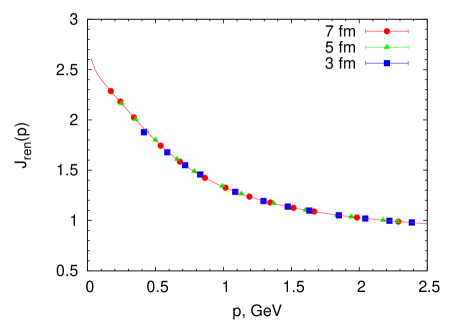
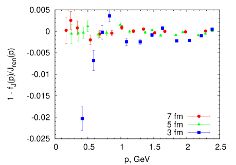
Figure 1: Left: The momentum dependence of the renormalized ghost dressing function $J_{ren}(p)$ for three different lattice sizes at $\beta=2.3$. The curve shows the fit applying Eq. (16) to the case $aL\simeq 7$ fm. Right: The relative deviation of the data for the ghost dressing function $J_{ren}(p)$ from the applied fitting curve.

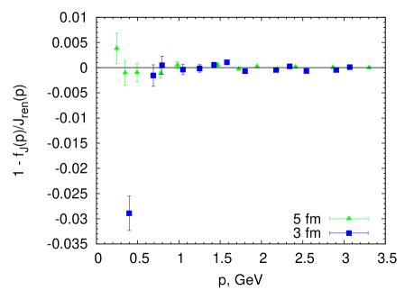
Figure 2: The same as in Fig. 1 but for two lattice sizes at $\beta=2.4$. The curve shows the fit applying Eq. (16) to the case $aL\simeq 5$ fm.

First let us discuss the finite volume effects for the renormalized ghost dressing function $J_{ren}(p,\mu)$. The data for various volumes are presented in Fig. 1 for $\beta=2.3$ and in Fig. 2 for $\beta=2.4$. To present the finite volume effects in more detail we fitted the data at $\beta=2.3$ for $aL\simeq 7$ fm and at $\beta=2.4$ for $aL\simeq 5$ fm with a fitting function of the form

$$f_{J}(p)=\frac{b_{1}}{\hat{p}^{2\kappa}}+\frac{b_{2}\hat{p}^{2}}{1+\hat{p}^{2}}$$ (16)

with the dimensionless rescaled momentum $\hat{p}\equiv p/m_{gh}$ (see Table 2). This ansatz, while describing the data reasonably well within the given momentum range, will not be applicable in the IR limit, when we assume that $J(p)$ exhibits an inflection point and bends to a finite value $J(0)$.

In the right panels of Fig. 1 and Fig. 2, respectively, the relative deviations from the fit function are shown for $\beta=2.3$ and $\beta=2.4$, respectively. One can see that for both $\beta$ values finite volume effects for lattices even with $aL\simeq 3$ fm are small (less than 1%) for momenta $|p|\,\mbox{}_{\textstyle\sim}^{\textstyle>}\,0.6$ GeV.

Now let us come to the discussion of lattice artifacts. In Fig. 3 (left) we show the momentum dependence of the renormalized ghost dressing function $J_{ren}(p)$ for five different lattice spacings but for (approximately) the same physical size $aL\simeq 3$ fm (for the exact values see Table 1). Finite-spacing effects for $\beta=2.2,2.3,2.4$ in comparison with $\beta=2.55$ are evident. The curve shows the fit function Eq. (16) for $\beta=2.55$ (see Table 2).

For every $\beta$ value we computed the ghost propagator for chosen values of the momentum in the range $0.41$ GeV $\leq p\leq 3.2$ GeV by interpolating the data using the function Eq. (16). For the interpolation 4 or 5 adjacent data points were used. For the purpose of this interpolation the choice of the function Eq. (16) was not really important. We then computed the ghost propagator in the continuum limit for these values of the momentum using a linear in $a^{2}$ extrapolation as shown in the right panel of Fig. 3. The data for the (comparably strong) coupling value $\beta=2.2$ were not used for the extrapolation and are not shown in this figure.

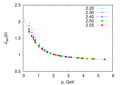
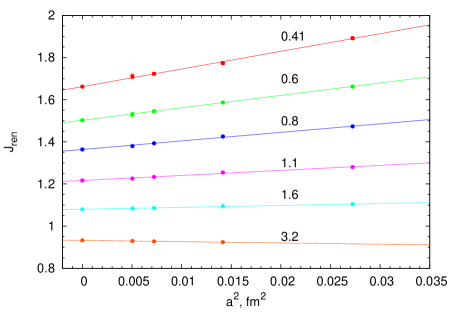
Figure 3: Left: The momentum dependence of the renormalized ghost dressing function $J_{ren}(p)$ for five different $\beta$-values or lattice spacings. The physical linear box size is $aL\simeq 3$ fm. The fitting curve belongs to the smallest available lattice spacing ($\beta=2.55$). Right: The continuum limit extrapolation for the ghost dressing function $J_{ren}(p)$. The lines show fits linear in $a^{2}$. The numbers indicate the momentum values $p$ in GeV. Corresponding points related to $\beta=2.2$ are not taken into account for the linear fit and, thus, not shown. The left most data points show the continuum extrapolated results.

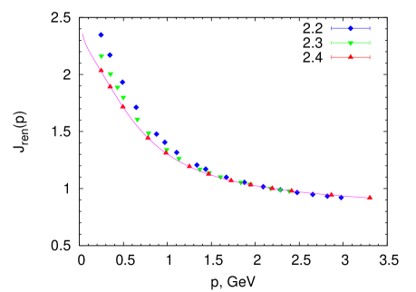
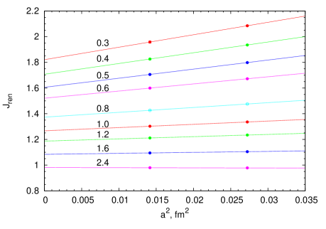
Figure 4: Left: Same as in Fig. 3 but for a linear box size of $aL\simeq 5$ fm and three different $\beta$-values. The fitting curve belongs to $\beta=2.40$. Right: Dressing function $J_{ren}(p)$ for few selected momenta as function of $a^{2}$. Data points related to the stronger coupling value $\beta=2.2$ are again discarded. The straight lines are only to guide the eye.

Related to our choice of the (re)normalization momentum $\mu=2.2$ GeV and due to the rather small statistical errors for the ghost dressing function we see clear scaling violations especially in the IR region but also for $p>\mu$. At the lowest (here accessible) momenta the violations at $\beta=2.3$ ($\beta=2.55$) relative to the continuum limit value are staying below $14\%$ ($3\%$).

Thus, in comparison with corresponding estimates for the gluon propagator (see Fig. 13 in Bornyakov et al. (2010)) which were more noisy, we can say that the relative scaling violations of the ghost dressing function turn out to be somewhat larger.

Similar to the case $aL\simeq 3$ fm we observe analogous lattice spacing effects on volumes with linear size $aL\simeq 5$ fm. The respective results are depicted in Fig. 4. As for the smaller volume we discard the data for $\beta=2.2$. Under these circumstances a real extrapolation to the continuum limit cannot be done. Nevertheless, Fig. 4 (right) clearly demonstrates finite lattice effects of a strength similar to the smaller volume case.

$\beta$	$L$	$m_{gh}~{}[GeV]$	$\kappa$	$b_{1}$	$b_{2}$	$\chi^{2}_{df}$
2.30	44	0.64(1)	0.026(1)	2.20(1)	-1.15(1)	1.8
2.40	42	0.67(1)	0.0232(4)	2.05(1)	-1.03(1)	1.9
2.55	42	0.696(15)	0.0215(4)	1.90(2)	-0.89(2)	2.27
c.l.1		0.743(5)	0.016(1)	1.827(5)	-0.85(1)	0.07
c.l.2		0.708(5)	0.027(1)	1.898(5)	-0.930(4)	0.04

Table 2: Values of the fit parameters according to Eq. (16) and the corresponding $\chi^{2}_{df}$. The last two lines correspond to fits of the extrapolated continuum limit values of the renormalized ghost dressing function in accordance with Eq. (16) and Eq. (17), respectively, for lattice size $aL\simeq 3$ fm.

Finally, let us present the continuum extrapolated result for the smaller volume of $aL\simeq 3$ fm in Fig. 5. We show the extracted points together with two fit curves: one with the ansatz Eq. (16) and the other with the alternative ansatz

$$f_{J}^{(2)}(p)=b_{1}+\frac{b_{2}\hat{p}^{2}}{(1+\hat{p}^{2})^{(1-\kappa)}},\qquad\hat{p}\equiv p/m_{gh}.$$ (17)

This function takes a nonzero value at $p=0$. We obtained good $\chi^{2}_{df}$ in both cases, 0.07 and 0.04, respectively. The parameters for both fitting curves are provided in the last two lines of Table 2.

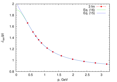
Figure 5: The momentum dependence of the renormalized ghost dressing function $J_{ren}(p)$ extracted in the continuum limit for selected momenta for $aL\simeq 3$ fm. The curves show fits with the ansatzes Eq. (16) and Eq. (17), respectively.

IV.2 Running coupling

Taking the gluon dressing function results from Bornyakov et al. (2010) into account we can compute the minimal MOM scheme running coupling von Smekal et al. (2009) via

$$\alpha_{s}(p)=\frac{g_{0}^{2}}{4\pi}Z(p)J(p)^{2}\,,$$ (18)

where $Z(p)$ and $J(p)$ are the bare gluon and ghost dressing functions, respectively.

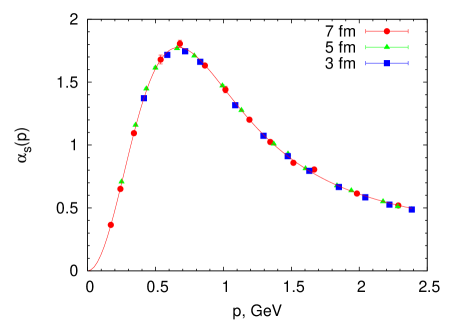
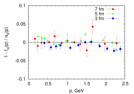
Figure 6: Left: The momentum dependence of the running coupling for three different lattice sizes at $\beta=2.3$. The curve shows a fit with Eq. (19) for $aL\simeq 7$ fm. Right: The relative deviation of the data for the running coupling $\alpha_{s}(p)$ from the fitting curve.

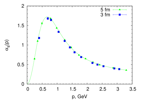
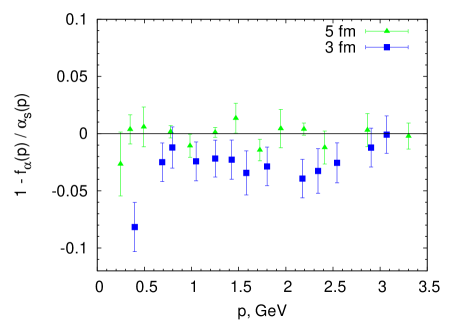
Figure 7: Same as in Fig. 6 but for two lattice sizes at $\beta=2.4$. The curve shows the fit result with Eq. (19) for $aL\simeq 5$ fm.

For the running coupling we use the following dimensionless fitting function:

$$f_{\alpha}(p)=\frac{c_{1}\hat{p}^{2}}{1+\hat{p}^{2}}+\frac{c_{2}\hat{p}^{2}}{(1+\hat{p}^{2})^{2}}+\frac{c_{3}\hat{p}^{2}}{(1+\hat{p}^{2})^{4}}\,,\quad\hat{p}\equiv p/m_{\alpha}\,.$$ (19)

The fit results for the same combinations of values $(\beta,~{}L)$ as for the ghost dressing function (see Table 2) are collected in Table 3.

Finite volume effects for the running coupling are shown in Fig. 6 for $\beta=2.3$ and in Fig. 7 for $\beta=2.4$. In both cases one can see the finite volume effects to be reasonably small (less than 5%) at a linear physical lattice extension $aL\simeq 3$ fm and for momenta $|p|\,\mbox{}_{\textstyle\sim}^{\textstyle>}\,0.6$ GeV.

Results for the scaling check of $\alpha_{s}(p)$ taking into account four lattice spacings for the same extent of $aL\simeq 3$ fm are presented in Fig. 8. We see relative deviations for $\beta=2.3$ in comparison with $\beta=2.55$ up to a $10\%$-level within the momentum range explored. Similar to the ghost dressing function we made extrapolations to the continuum limit for selected momenta. The running coupling for these selected momenta as a linear function of $a^{2}$ is shown in the right panel of Fig. 8 together with extrapolations to the $a=0$ limit. One can see that finite lattice spacing effects are very strong at $\beta=2.3$. The respective data were not included into the continuum extrapolation. Another feature seen from this figure is that the sign of the scaling violation effects changes twice: it is negative to the left from the maximum of $\alpha_{s}(p)$ ($p=0.41$ GeV and $0.6$ GeV), becomes positive right above it ($p=0.8$ MeV and $1.0$ MeV) and then again turns negative. In the range of momenta $p>1.2$ GeV the effect is rather stable in strength up to our maximal momentum value.

In Fig. 9 we present our results for the continuum values of the running coupling $\alpha_{s}(p)$ for linear size $aL\simeq 3$ fm. For the fit the same ansatz according to Eq. (19) was used. The fit parameters are included in Table 3 (as the last line).

Since the running coupling $\alpha_{s}$ seems to tend to zero in the IR limit, our results obtained within the framework of Landau gauge fixing as described above are fully compatible with the IR-decoupling scenario discussed in the context of the Dyson-Schwinger and functional renormalization group approach Fischer et al. (2009); Boucaud et al. (2012).

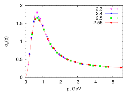
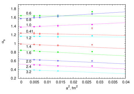
Figure 8: Left: The momentum dependence of the running coupling for four different $\beta$-values or lattice spacings at lattice extent $aL\simeq 3$ fm. The curve shows the fit result with Eq. (19) for $\beta=2.55$. Right: The extrapolation to the continuum limit with a function linear in $a^{2}$ for selected momenta (in GeV).

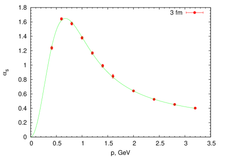
Figure 9: The momentum dependence of the running coupling $\alpha_{s}(p)$ extracted in the continuum limit for selected momenta and $aL\simeq 3$ fm. The curve shows a fit corresponding to the ansatz Eq. (19).

$\beta$	$L$	$m_{\alpha}$ [GeV]	$c_{1}$	$c_{2}$	$c_{3}$	$\chi^{2}_{df}$
2.30	44	1.03(1)	0.19(4)	2.3(2)	12(2)	0.95
2.40	42	1.01(1)	0.16(1)	2.63(5)	11.0(7)	0.81
2.55	42	1.04(1)	0.205(3)	2.29(3)	11.0(7)	1.3
c.l.		1.01(2)	0.199(15)	2.56(8)	10.0(1.1)	0.57

Table 3: Values of the fit parameters for $\alpha_{s}$ (Eq. (19)) and the corresponding $\chi^{2}_{df}$. The last line collects the corresponding fit parameter values in the continuum limit extrapolated case for a linear lattice size of $3$ fm.

V Conclusions

Completing an earlier work Bornyakov et al. (2010) we have computed the Landau gauge ghost dressing function for lattice $SU(2)$ pure gauge theory. In combination with the former results for the gluon propagator we have now presented the running coupling in the minimal MOM scheme. We have employed the same sets of gauge-fixed field configurations as analysed in Bornyakov et al. (2010). They had been obtained with a gauge fixing method consisting of a combined application of $Z(2)$-flips and repeated simulated annealing with subsequent overrelaxation for the gauge functional. This method was used in order to get as close as possible to the fundamental modular region i.e. to the global extremum of the gauge functional, by choosing among ${\cal O}(50-80)$ copies. It previously was suggested to provide a possible solution for the Gribov problem with suppressed finite size effects Bogolubsky et al. (2008, 2007).

Assuming that the Gribov problem is kept under control to the best of our present knowledge, we concentrated ourselves on systematic effects like finite size and lattice spacing dependences. While finite size effects were confirmed to be rather small, the lattice spacing artifacts turned out to be non-negligible as well for the renormalized ghost dressing function as for the running coupling. In both cases for a linear lattice size of approximately $aL\simeq 3$ fm (and for the ghost dressing function with a subtraction momentum of $\mu=2.2$ GeV) we have seen relative deviations at $\beta=2.30$ from the results obtained at our largest $\beta=2.55$ reaching a ten percent level at the lowest accessible momentum values and still around five percent in the non-perturbative region around 1 GeV. This tells us that lattice results for Landau gauge gluon and ghost propagators in this momentum range have still to be taken with some caution what concerns the Gribov problem and the continuum limit.

Consequently we tried an extrapolation to the continuum limit for the $aL\simeq 3$ fm volume, where we could rely on several values of the lattice spacing. We did this with fixed physical momenta chosen between $0.41$ GeV and $3.2$ GeV. We presented fit formulae for the continuum limit of the ghost dressing function as well as of the running coupling valid in this range. For momenta above $0.6$ GeV we have seen that also finite volume effects are under control.

Although the ghost dressing function in the restricted momentum range has been equally well fitted by a weakly IR singular behavior (see Eq. (16)) or with an IR regular ansatz Eq. (17), thus leaving open an IR finite limit, the result for the running coupling $\alpha_{s}(p)$ turned out to be robust, what emphasizes the compatibility with the infrared decoupling solution of Dyson-Schwinger and functional renormalization group equations.

Acknowledgments

This investigation has been partly supported by the Heisenberg-Landau program of collaboration between the Bogoliubov Laboratory of Theoretical Physics of the Joint Institute for Nuclear Research Dubna (Russia) and German institutes and partly by the DFG grant Mu 932/7-1. V.G.B. acknowledges support by RFBR grant 11-02-01227-a and jointly with V.K.M. by RFBR grant 13-02-01387-a.

References

- Gribov (1978) V. N. Gribov, Nucl. Phys. B139, 1 (1978).
- Kugo and Ojima (1979) T. Kugo and I. Ojima, Prog. Theor. Phys. Suppl. 66, 1 (1979).
- Zwanziger (1991) D. Zwanziger, Nucl. Phys. B364, 127 (1991).
- Zwanziger (2002) D. Zwanziger, Phys. Rev. D65, 094039 (2002), eprint hep-th/0109224.
- Zwanziger (2009) D. Zwanziger (2009), eprint 0904.2380.
- von Smekal et al. (1997) L. von Smekal, R. Alkofer, and A. Hauck, Phys. Rev. Lett. 79, 3591 (1997), eprint hep-ph/9705242.
- von Smekal et al. (1998) L. von Smekal, A. Hauck, and R. Alkofer, Ann. Phys. 267, 1 (1998), eprint hep-ph/9707327.
- Alkofer and von Smekal (2001) R. Alkofer and L. von Smekal, Phys. Rept. 353, 281 (2001), eprint hep-ph/0007355.
- Alkofer et al. (2003) R. Alkofer, C. S. Fischer, and L. von Smekal, Eur. Phys. J. A17, 773 (2003), eprint hep-ph/0209366.
- Fischer and Alkofer (2002) C. S. Fischer and R. Alkofer, Phys. Lett. B536, 177 (2002), eprint hep-ph/0202202.
- Fischer et al. (2002) C. S. Fischer, R. Alkofer, and H. Reinhardt, Phys. Rev. D65, 094008 (2002), eprint hep-ph/0202195.
- Pawlowski et al. (2004) J. M. Pawlowski, D. F. Litim, S. Nedelko, and L. von Smekal, Phys. Rev. Lett. 93, 152002 (2004), eprint hep-th/0312324.
- Alkofer et al. (2005) R. Alkofer, C. S. Fischer, and F. J. Llanes-Estrada, Phys. Lett. B611, 279 (2005), eprint hep-th/0412330.
- Fischer and Pawlowski (2007) C. S. Fischer and J. M. Pawlowski, Phys. Rev. D75, 025012 (2007), eprint hep-th/0609009.
- Boucaud et al. (2007) P. Boucaud, J. P. Leroy, A. Le Yaouanc, A. Y. Lokhov, J. Micheli, O. Pene, J. Rodriguez-Quintero, and C. Roiesnel, Eur. Phys. J. A31, 750 (2007), eprint hep-ph/0701114.
- Boucaud et al. (2008a) P. Boucaud, J.-P. Leroy, A. L. Yaouanc, J. Micheli, O. Pene, and J. Rodriguez-Quintero, JHEP 06, 012 (2008a), eprint 0801.2721.
- Boucaud et al. (2008b) P. Boucaud, J. P. Leroy, A. Le Yaouanc, J. Micheli, O. Pene, and J. Rodriguez-Quintero, JHEP 06, 099 (2008b), eprint 0803.2161.
- Aguilar et al. (2008) A. C. Aguilar, D. Binosi, and J. Papavassiliou, Phys. Rev. D78, 025010 (2008), eprint 0802.1870.
- Pennington and Wilson (2011) M. Pennington and D. Wilson, Phys.Rev. D84, 119901 (2011), eprint 1109.2117.
- Fischer et al. (2009) C. S. Fischer, A. Maas, and J. M. Pawlowski, Annals Phys. 324, 2408 (2009), eprint 0810.1987.
- Braun et al. (2010) J. Braun, H. Gies, and J. M. Pawlowski, Phys. Lett. B684, 262 (2010), eprint 0708.2413.
- Dudal et al. (2008a) D. Dudal, S. P. Sorella, N. Vandersickel, and H. Verschelde, Phys. Rev. D77, 071501 (2008a), eprint 0711.4496.
- Dudal et al. (2008b) D. Dudal, J. A. Gracey, S. P. Sorella, N. Vandersickel, and H. Verschelde, Phys. Rev. D78, 065047 (2008b), eprint 0806.4348.
- Alkofer (2007) R. Alkofer, Braz. J. Phys. 37, 144 (2007), eprint hep-ph/0611090.
- Eichmann et al. (2009) G. Eichmann, I. C. Cloet, R. Alkofer, A. Krassnigg, and C. D. Roberts, Phys. Rev. C79, 012202 (2009), eprint 0810.1222.
- Sternbeck et al. (2012) A. Sternbeck, K. Maltman, M. Müller-Preussker, and L. von Smekal, PoS LATTICE2012, 243 (2012), eprint 1212.2039.
- Burger et al. (2013) F. Burger, V. Lubicz, M. Müller-Preussker, S. Simula, and C. Urbach, Phys. Rev. D87, 034514 (2013), eprint 1210.0838.
- Chetyrkin (2005) K. G. Chetyrkin, Nucl. Phys. B710, 499 (2005), eprint hep-ph/0405193.
- Chetyrkin and Maier (2009) K. G. Chetyrkin and A. Maier (2009), eprint 0911.0594.
- Mandula and Ogilvie (1987) J. E. Mandula and M. Ogilvie, Phys. Lett. B185, 127 (1987).
- Suman and Schilling (1996) H. Suman and K. Schilling, Phys. Lett. B373, 314 (1996), eprint hep-lat/9512003.
- Leinweber et al. (1999) D. B. Leinweber, J. I. Skullerud, A. G. Williams, and C. Parrinello (UKQCD), Phys. Rev. D60, 094507 (1999), eprint hep-lat/9811027.
- Becirevic et al. (1999) D. Becirevic, P. Boucaud, J. P. Leroy, J. Micheli, O. Pene, J. Rodriguez-Quintero, and C. Roiesnel, Phys. Rev. D60, 094509 (1999), eprint hep-ph/9903364.
- Becirevic et al. (2000) D. Becirevic, P. Boucaud, J. P. Leroy, J. Micheli, O. Pene, J. Rodriguez-Quintero, and C. Roiesnel, Phys. Rev. D61, 114508 (2000), eprint hep-ph/9910204.
- Bonnet et al. (2000) F. D. R. Bonnet, P. O. Bowman, D. B. Leinweber, and A. G. Williams, Phys. Rev. D62, 051501 (2000), eprint hep-lat/0002020.
- Bonnet et al. (2001) F. D. R. Bonnet, P. O. Bowman, D. B. Leinweber, A. G. Williams, and J. M. Zanotti, Phys. Rev. D64, 034501 (2001), eprint hep-lat/0101013.
- Bloch et al. (2003) J. C. R. Bloch, A. Cucchieri, K. Langfeld, and T. Mendes, Nucl. Phys. Proc. Suppl. 119, 736 (2003), eprint hep-lat/0209040.
- Bloch et al. (2004) J. C. R. Bloch, A. Cucchieri, K. Langfeld, and T. Mendes, Nucl. Phys. B687, 76 (2004), eprint hep-lat/0312036.
- Furui and Nakajima (2004a) S. Furui and H. Nakajima, Phys. Rev. D69, 074505 (2004a), eprint hep-lat/0305010.
- Boucaud et al. (2005) P. Boucaud, J. P. Leroy, A. Le Yaouanc, A. Y. Lokhov, J. Micheli, O. Pene, J. Rodriguez-Quintero, and C. Roiesnel, Phys. Rev. D72, 114503 (2005), eprint hep-lat/0506031.
- Sternbeck et al. (2005) A. Sternbeck, E.-M. Ilgenfritz, M. Müller-Preussker, and A. Schiller, Phys. Rev. D72, 014507 (2005), eprint hep-lat/0506007.
- Bowman et al. (2007) P. O. Bowman, U. M. Heller, D. B. Leinweber, M. B. Parappilly, A. Sternbeck, L. von Smekal, A. G. Williams, and J. Zhang, Phys. Rev. D76, 094505 (2007), eprint hep-lat/0703022.
- Cucchieri and Mendes (2007) A. Cucchieri and T. Mendes, PoS LAT2007, 297 (2007), eprint 0710.0412.
- Cucchieri and Mendes (2008a) A. Cucchieri and T. Mendes, Phys.Rev.Lett. 100, 241601 (2008a), eprint 0712.3517.
- Cucchieri et al. (2007) A. Cucchieri, T. Mendes, O. Oliveira, and P. Silva, Phys.Rev. D76, 114507 (2007), eprint 0705.3367.
- Sternbeck et al. (2007) A. Sternbeck, L. von Smekal, D. B. Leinweber, and A. G. Williams, PoS LAT2007, 340 (2007), eprint 0710.1982.
- Cucchieri and Mendes (2008b) A. Cucchieri and T. Mendes, Phys.Rev. D78, 094503 (2008b), eprint 0804.2371.
- Oliveira and Silva (2009) O. Oliveira and P. J. Silva, Phys. Rev. D79, 031501 (2009), eprint 0809.0258.
- Bogolubsky et al. (2009) I. L. Bogolubsky, E.-M. Ilgenfritz, M. Müller-Preussker, and A. Sternbeck, Phys. Lett. B676, 69 (2009), eprint 0901.0736.
- Oliveira and Silva (2012) O. Oliveira and P. J. Silva, Phys. Rev. D86, 114513 (2012), eprint 1207.3029.
- Maas (2015) A. Maas, Phys.Rev. D91, 034502 (2015), eprint 1402.5050.
- Cucchieri (1997) A. Cucchieri, Nucl. Phys. B508, 353 (1997), eprint hep-lat/9705005.
- Bakeev et al. (2004) T. D. Bakeev, E.-M. Ilgenfritz, V. K. Mitrjushkin, and M. Müller-Preussker, Phys. Rev. D69, 074507 (2004), eprint hep-lat/0311041.
- Furui and Nakajima (2004b) S. Furui and H. Nakajima, AIP Conf. Proc. 717, 685 (2004b), [,685(2003)], eprint hep-lat/0309166.
- Silva and Oliveira (2004) P. J. Silva and O. Oliveira, Nucl. Phys. B690, 177 (2004), eprint hep-lat/0403026.
- Furui and Nakajima (2004c) S. Furui and H. Nakajima, Phys. Rev. D70, 094504 (2004c).
- Bogolubsky et al. (2006) I. L. Bogolubsky, G. Burgio, V. K. Mitrjushkin, and M. Müller-Preussker, Phys. Rev. D74, 034503 (2006), eprint hep-lat/0511056.
- Bornyakov et al. (2009) V. G. Bornyakov, V. K. Mitrjushkin, and M. Müller-Preussker, Phys. Rev. D79, 074504 (2009), eprint 0812.2761.
- Maas (2009) A. Maas, Phys. Rev. D79, 014505 (2009), eprint 0808.3047.
- Maas et al. (2010) A. Maas, J. M. Pawlowski, D. Spielmann, A. Sternbeck, and L. von Smekal, Eur. Phys. J. C68, 183 (2010), eprint 0912.4203.
- Hughes et al. (2013) C. Hughes, D. Mehta, and J.-I. Skullerud, Annals Phys. 331, 188 (2013), eprint 1203.4847.
- Maas (2010) A. Maas, Phys. Lett. B689, 107 (2010), eprint 0907.5185.
- Sternbeck and Müller-Preussker (2013) A. Sternbeck and M. Müller-Preussker, Phys.Lett. B726, 396 (2013), eprint 1211.3057.
- Zwanziger (2013) D. Zwanziger, Phys.Rev. D87, 085039 (2013), eprint 1209.1974.
- Cucchieri et al. (2012) A. Cucchieri, D. Dudal, and N. Vandersickel, Phys.Rev. D85, 085025 (2012), eprint 1202.1912.
- von Smekal et al. (2008) L. von Smekal, A. Jorkowski, D. Mehta, and A. Sternbeck, PoS CONFINEMENT8, 048 (2008), eprint 0812.2992.
- Burgio et al. (2010) G. Burgio, M. Quandt, and H. Reinhardt, Phys. Rev. D81, 074502 (2010), eprint 0911.5101.
- Cucchieri et al. (2014a) A. Cucchieri, D. Dudal, T. Mendes, and N. Vandersickel, Phys.Rev. D90, 051501 (2014a), eprint 1405.1547.
- Cucchieri et al. (2014b) A. Cucchieri, D. Dudal, T. Mendes, and N. Vandersickel, PoS LATTICE2014, 347 (2014b), eprint 1410.8410.
- Bornyakov et al. (2010) V. G. Bornyakov, V. K. Mitrjushkin, and M. Müller-Preussker, Phys. Rev. D81, 054503 (2010), eprint 0912.4475.
- von Smekal et al. (2009) L. von Smekal, K. Maltman, and A. Sternbeck, Phys. Lett. B681, 336 (2009), eprint 0903.1696.
- Zwanziger (1994) D. Zwanziger, Nucl. Phys. B412, 657 (1994).
- Fingberg et al. (1993) J. Fingberg, U. M. Heller, and F. Karsch, Nucl. Phys. B392, 493 (1993), eprint hep-lat/9208012.
- Lucini and Teper (2001) B. Lucini and M. Teper, JHEP 0106, 050 (2001), eprint hep-lat/0103027.
- Bogolubsky et al. (2008) I. L. Bogolubsky, V. G. Bornyakov, G. Burgio, E.-M. Ilgenfritz, V. K. Mitrjushkin, and M. Müller-Preussker, Phys. Rev. D77, 014504 (2008), eprint 0707.3611.
- Schemel (2006) P. Schemel, Diploma thesis, Humboldt University Berlin, Germany, see http://pha.physik.hu-berlin.de - Theses (2006).
- Bogolubsky et al. (2007) I. L. Bogolubsky, V. G. Bornyakov, G. Burgio, E.-M. Ilgenfritz, V. K. Mitrjushkin, M. Müller-Preussker, and P. Schemel, PoS LAT2007, 318 (2007), eprint 0710.3234.
- Nakagawa et al. (2009) Y. Nakagawa, A. Voigt, E.-M. Ilgenfritz, M. Müller-Preussker, A. Nakamura, T. Saito, A. Sternbeck, and H. Toki, Phys. Rev. D79, 114504 (2009), eprint 0902.4321.
- Boucaud et al. (2012) P. Boucaud, J. P. Leroy, A. L. Yaouanc, J. Micheli, O. Pene, and J. Rodriguez-Quintero, Few Body Syst. 53, 387 (2012), eprint 1109.1936.