Delta and Omega electromagnetic form factors in a three-body covariant Bethe-Salpeter approach

Abstract

The electromagnetic form factors of the $\Delta$ and $\Omega$ baryons are calculated in the framework of Poincaré-covariant bound-state equations. The quark-quark interaction is truncated to a single dressed-gluon exchange where for the dressings we use two different models and compare the results. The calculation predicts an oblate shape for the electric charge distribution and a prolate shape for the magnetic dipole distribution. We also identify the necessity of including pion-cloud corrections at low photon-momentum transfer.

I Introduction

The spatial distribution of hadrons’ extensive properties, such as mass or electric charge, is of especial relevance in the understanding of low-energy QCD dynamics, since they probe the details of the quark-quark and gluon-quark interactions.

The electromagnetic properties of the proton have been widely studied experimentally, providing a good picture of its internal structure. This is not the case, however, for the lightest baryonic resonance, the $\Delta(1232)$. Its short lifetime makes the study of its properties difficult and only the magnetic moments of $\Delta^{++}$ Nefkens:1977eb ; Heller:1986gn ; Wittman:1987kb ; Lin:1991tx ; Lin:1991qk ; Bosshard:1990ys ; Bosshard:1991zp ; LopezCastro:2000cv ; LopezCastro:2000ep ; Beringer:1900zz and $\Delta^{+}$ Beringer:1900zz ; Kotulla:2002cg are known, albeit with large errors. An indirect estimation of the $\Delta^{+}$ electric quadrupole moment from the $\gamma N\rightarrow\Delta$ transition quadrupole moment was given in Blanpied:2001ae . The $\Omega(1672)$ decays weakly, instead, and this has allowed for a precise measurement of its magnetic dipole moment Beringer:1900zz .

For finite values of the photon momentum the only information available comes from lattice QCD calculations Alexandrou:2009hs ; Alexandrou:2009nj ; Alexandrou:2010jv ; Aubin:2008qp ; Boinepalli:2009sq . Although constantly improving, these calculations suffer from the usual problem of not yet being able to work at the physical pion mass. Moreover, the limit of vanishing photon momentum is unreachable for technical reasons. The calculation of the electromagnetic properties of the Delta and Omega baryons has also been tackled from a number of constituent quark models Ramalho:2008dc ; Ramalho:2009vc ; Ramalho:2010xj ; Ramalho:2010rr , chiral quark-soliton model Ledwig:2008es , chiral perturbation theory Geng:2009ys ; Ledwig:2011cx and QCD sum rules Azizi:2008tx .

In this paper, we investigate the electromagnetic properties of the Delta and Omega baryon in the framework of covariant Bethe-Salpeter equations. In section II we introduce the general formalism of Bethe-Salpeter equations (BSE) and Dyson-Schwinger equations (DSE). This is followed by a presentation of the truncation used in section III. In section IV the results of our calculation are discussed. Finally, we conclude in section V.

II Baryon Bethe-Salpeter equation and coupling to an external field

The evolution of a three-quark system in quantum field theory is described through the six-quark Green’s function $G^{(3)}(p_{1},p_{2},p_{3})$ (in momentum space) or, equivalently, its amputated version the scattering matrix $T^{(3)}(p_{1},p_{2},p_{3})$. This function can be obtained by solving a Dyson equation

$$T=-iK-iKG_{0}T~{},$$ (1)

or, equivalently,

$$T^{-1} =iK^{-1}-G_{0}\,\,,$$ (2)

$$\mathbb{1} =iTK^{-1}-TG_{0}\,\,,$$ (3)

where $G_{0}$ is the disconnected product of three full quark propagators and $-iK$ is the three-quark interaction kernel. The latter includes three- and two-particle irreducible interactions

$$K\equiv\widetilde{K}^{(3)}+\sum_{a=1}^{3}\widetilde{K}^{(2)}_{a}S^{-1}_{a}\,\,,$$ (4)

with $a$ denoting the spectator quark (see e.g. Fig. 2). The full quark propagator $S$ is obtained by solving the quark propagator DSE (see Fig. 1)

$$S^{-1}(p)=S^{-1}_{0}(p)+Z_{1f}\int_{q}\gamma^{\mu}D_{\mu\nu}(p-q)\Gamma^{\nu}_{gqq}(p,q)S(q)\,\,,$$ (5)

where $S_{0}$ is the (renormalized) bare propagator

$$S^{-1}_{0}(p)=Z_{2}\left(i\ooalign{\hfil/\hfil\crcr$p$}+m\right)\,\,,$$ (6)

$\Gamma^{\nu}_{gqq}$ is the full quark-gluon vertex and $D^{\mu\nu}$ is the full gluon propagator and $Z_{1f}$ and $Z_{2}$ are renormalization constants. In the Landau gauge the gluon propagator takes the form

$$D^{\mu\nu}(k)=T^{\mu\nu}(k)\frac{Z(k^{2})}{k^{2}}~{},$$ (7)

with $Z(k^{2})$ a dressing function to be determined and $T^{\mu\nu}$ the transverse projector

$$T_{\mu\nu}(k)=\delta_{\mu\nu}-\frac{k_{\mu}k_{\nu}}{k^{2}}\,\,.$$ (8)

The bare quark mass $m$ in (6) must be provided as a parameter.

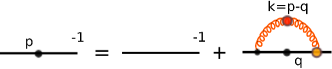
Figure 1: Diagrammatic representation of the quark Dyson-Schwinger equation (5). Blobs represent fully dressed propagators or vertices.

When the three-quark system forms a bound state, the Green’s function $T^{(3)}$ develops a pole at $P^{2}=-M^{2}$, with $P$ the total quark momentum

$$P=p_{1}+p_{2}+p_{3}\,\,,$$ (9)

and $p_{i}$ the quark momenta, with $M$ the bound-state mass. At the bound state pole one defines

$$T^{(3)}\sim\mathcal{N}\frac{\Psi\bar{\Psi}}{P^{2}+M^{2}}~{},$$ (10)

where $\mathcal{N}$ is a normalization factor which, in the case of spin-$\nicefrac{{3}}{{2}}$ particles is $2M$. The function $\Psi$ is the bound-state Bethe-Salpeter amplitude and $\bar{\Psi}$ its charge conjugate. They are expressed as tensor products of flavor, color and spin parts which describe a baryon in terms of its constituent quarks. For spin-$\nicefrac{{3}}{{2}}$ baryons the spin part is itself a mixed tensor with four Dirac indices and one Lorentz index SanchisAlepuz:2010in ; SanchisAlepuz:2011jn ; SanchisAlepuz:2012vb . Substituting (10) in (2) or in (3), and keeping only the singular terms, we arrive at the Bethe-Salpeter equation for the three-quark bound state

$$\Psi=-iKG_{0}\Psi\,\,,$$ (11)

or

$$i\bar{\Psi}K^{-1}=\bar{\Psi}G_{0}\,\,.$$ (12)

A systematic procedure to couple an external gauge field to the constituents of a three-particle system described by integral equations is the so-called gauging of the equations, introduced in Haberzettl:1997jg ; Kvinikhidze:1998xn ; Kvinikhidze:1999xp ; Oettel:1999gc . It ensures that the resulting equations are gauge invariant and that there is no over-counting of diagrams. For our purposes it suffices to say that the gauging of equations acts as a derivative on the integral equation. That is, (1) becomes

$$T^{\mu}= ~{}-iK^{\mu}-iK^{\mu}G_{0}T$$

$$~{}-iKG^{\mu}_{0}T-iKG_{0}T^{\mu}\,\,,$$ (13)

where the superindex $\mu$ denotes a gauged function (that is, coupled to the gauge field). This equation can be rewritten, using (1), as

$$T^{\mu}= ~{}(1+iKG_{0})^{-1}\times$$

$$\left(-iK^{\mu}-iK^{\mu}G_{0}T-iKG^{\mu}_{0}T\right)$$

$$= ~{}T\left(iK^{-1}K^{\mu}K^{-1}+G^{\mu}_{0}\right)T~{}.$$ (14)

To have an expression for $K^{\mu}$ one needs to specify the interaction kernel. In the next section we shall obtain the gauged kernel in the case of the Rainbow-Ladder truncation. The gauged quark propagator allows the introduction of the proper vertex $\Gamma^{\mu}$ through the definition

$$S^{\mu}=S\Gamma^{\mu}S\,\,,$$ (15)

which, in the case that concerns us in this paper, represents the fully dressed quark-photon vertex.

The bound-state electromagnetic current $J^{\mu}$ can be introduced at the bound-state pole by

$$T^{(3),\mu}\sim\mathcal{N}_{i}\mathcal{N}_{f}\frac{\Psi_{f}}{P_{f}^{2}+M_{f}^{2}}J^{\mu}\frac{\bar{\Psi}_{i}}{P_{i}^{2}+M_{i}^{2}}\,\,.$$ (16)

Substituting in (II) and using (11) and (12) we arrive at

$$J^{\mu}= ~{}\bar{\Psi}_{f}\left(-iG_{0}K^{\mu}G_{0}+G^{\mu}_{0}\right)\Psi_{i}\,\,.$$ (17)

The electromagnetic form factors are calculated via the identification of (17) with the expression of the current imposed by symmetry principles (see Appendix A).

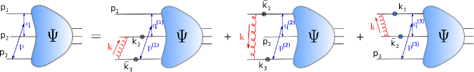
Figure 2: Diagrammatic representation of the covariant Faddeev equation in the Rainbow-Ladder truncation (III.1).

III Rainbow-Ladder truncation

To solve (11) one needs to specify the interaction kernel $K$. An exact expression for this kernel is in general not available and one has to resort to some truncation scheme. The simplest consistent scheme is known as Rainbow-Ladder (RL) truncation. This truncation preserves the axial-vector Ward-Takahashi identity, which relates the quark-antiquark interaction kernel and the quark-gluon vertex in the quark DSE Munczek:1994zz ; Bender:1996bb . In the meson sector this identity ensures that pions are the Goldstone bosons of spontaneous chiral symmetry breaking Maris:1997hd . The RL truncation reduces the quark-antiquark kernel to a single dressed-gluon exchange. The full quark-gluon vertex is projected onto the tree-level Lorentz structure $\gamma^{\mu}$ and the non-perturbative dressing is restricted to depend on the gluon momentum only and has to be modelled. It is customary to include this dressing and the gluon propagator dressing $Z(k^{2})$ in a single effective interaction $\alpha(k^{2})$.

III.1 Three-quark bound state equations

Interactions in the baryon sector are not restricted, in principle, by the axial-vector Ward-Takahashi identity. However, we adopt here for the quark-quark interaction kernel the same truncation scheme and neglect the three-particle irreducible interactions. The three-body BSE (11) in the RL truncation, which is also known as covariant Faddeev equation (and, correspondingly, the Bethe-Salpeter amplitudes $\Psi$ are called Faddeev amplitudes), reads (see Fig. 2)

$$\Psi_{\alpha\beta\gamma\mathcal{I}}(p,q,P)={} \int_{k}\left[\widetilde{K}_{\beta\beta^{\prime}\gamma\gamma^{\prime}}(k)~{}S_{\beta^{\prime}\beta^{\prime\prime}}(k_{2})S_{\gamma^{\prime}\gamma^{\prime\prime}}(\tilde{k}_{3})~{}\Psi_{\alpha\beta^{\prime\prime}\gamma^{\prime\prime}\mathcal{I}}(p^{(1)},q^{(1)},P)\right.$$

$$\quad\left.+\widetilde{K}_{\alpha\alpha^{\prime}\gamma\gamma^{\prime}}(-k)~{}S_{\gamma^{\prime}\gamma^{\prime\prime}}(k_{3})S_{\alpha^{\prime}\alpha^{\prime\prime}}(\tilde{k}_{1})~{}\Psi_{\alpha^{\prime\prime}\beta\gamma^{\prime\prime}\mathcal{I}}(p^{(2)},q^{(2)},P)\right.$$

$$\quad\left.+\widetilde{K}_{\alpha\alpha^{\prime}\beta\beta^{\prime}}(k)~{}S_{\alpha^{\prime}\alpha^{\prime\prime}}(k_{1})S_{\beta^{\prime}\beta^{\prime\prime}}(\tilde{k}_{2})~{}\Psi_{\alpha^{\prime\prime}\beta^{\prime\prime}\gamma\mathcal{I}}(p^{(3)},q^{(3)},P)\right]\,\,,$$ (18)

where we have absorbed the $-i$ factor into the definition of $\widetilde{K}$, so that it is defined as

$$\widetilde{K}_{\alpha\alpha^{\prime}\beta\beta^{\prime}}(k)=-4\pi C~{}Z_{2}^{2}~{}\frac{\alpha_{\textrm{eff}}(k^{2})}{k^{2}}~{}T_{\mu\nu}(k)~{}\gamma^{\mu}_{\alpha\alpha^{\prime}}\gamma^{\nu}_{\beta\beta^{\prime}}\,\,,$$ (19)

with $Z_{2}$ the quark renormalization constant. We have used the generic index $\mathcal{I}$ to refer to the bound state (as opposed to the first three Greek indices in the Faddeev amplitude which denote the valence quarks); for the case of a spin-$\nicefrac{{3}}{{2}}$ baryon $\mathcal{I}$ consists of a Dirac and a Lorentz index. In (III.1), the flavor part of the Faddeev amplitudes has been factored out because the interaction kernel is flavor-independent and the factor $C=-2/3$  stems from the traces of the color structures. The Faddeev amplitudes depend on the quark momenta $p_{1}$, $p_{2}$ and $p_{3}$, but this dependence can be reexpressed in terms of the total momentum $P$ and two relative momenta $p$ and $q$

$$p =(1-\zeta)\,p_{3}-\zeta(p_{1}+p_{2})\,, p_{1} =-q-\dfrac{p}{2}+\dfrac{1-\zeta}{2}P\,,$$

$$q =\dfrac{p_{2}-p_{1}}{2}\,, p_{2} =q-\dfrac{p}{2}+\dfrac{1-\zeta}{2}P\,,$$

$$P =p_{1}+p_{2}+p_{3}\,, p_{3} =p+\zeta P\,\,,$$

with $\zeta$ a free momentum partitioning parameter, which we choose $\zeta=1/3$ for numerical convenience. The internal quark propagators depend on the internal quark momenta $k_{i}=p_{i}-k$ and $\tilde{k}_{i}=p_{i}+k$, with $k$ the gluon momentum. The internal relative momenta, for each of the three terms in the Faddeev equation, are

$$p^{(1)} =p+k, p^{(2)} =p-k, p^{(3)} =p,$$

$$q^{(1)} =q-k/2, q^{(2)} =q-k/2, q^{(3)} =q+k\,\,.$$

The quark DSE in the RL truncation reduces to

$$S^{-1}_{\alpha^{\prime}\beta^{\prime}}(p)=S_{0,\alpha^{\prime}\beta^{\prime}}(p)+\int_{q}\widetilde{K}_{\alpha\alpha^{\prime}\beta\beta^{\prime}}(k)S_{\alpha^{\prime}\beta^{\prime}}(q)\,\,,$$ (22)

where now in $\widetilde{K}$, see (19), we have $C=4/3$ and $k=p-q$.

III.2 Bound state electromagnetic current and quark-photon vertex

The expression for the current (17) simplifies considerably in the RL truncation. Since $\widetilde{K}^{(3)}$ is absent and $\widetilde{K}^{(2)}$ is reduced to the exchange of a neutral particle, the photon can only couple to the quark propagator through the term $S^{-1}$ in (4). Defining $\mathbb{1}^{\mu}=(SS^{-1})^{\mu}=0$ we obtain

$$\left(S^{-1}\right)^{\mu}=-S^{-1}S^{\mu}S^{-1}=-\Gamma^{\mu}\,\,,$$ (23)

where we used (15). Thus (17) becomes (cf. Fig. 3)

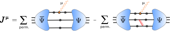
Figure 3: Diagrammatic representation of the current (17) in the Rainbow-Ladder truncation, see Eq. (III.2).

$$J_{\mathcal{I}^{\prime}\mathcal{I}}^{\mu}=\int_{p}\int_{q}\bar{\Psi}_{\beta^{\prime}\alpha^{\prime}\mathcal{I}^{\prime}\gamma^{\prime}}(p_{f}^{\{1\}},q^{\{1\}}_{f},P_{f})\left[\left(S(p_{1}^{f})\Gamma^{\mu}(p_{1},Q)S(p_{1}^{i})\right)_{\alpha^{\prime}\alpha}S_{\beta^{\prime}\beta}(p_{2})S_{\gamma^{\prime}\gamma}(p_{3})\right]\times$$

$$~{}~{}~{}~{}~{}~{}~{}~{}~{}~{}~{}~{}~{}~{}~{}~{}~{}~{}~{}~{}~{}~{}~{}~{}~{}~{}~{}~{}~{}~{}\left(\Psi_{\alpha\beta\gamma\mathcal{I}}(p^{\{1\}}_{i},q^{\{1\}}_{i},P_{i})-\Psi^{\{1\}}_{\alpha\beta\gamma\mathcal{I}}(p^{\{1\}}_{i},q^{\{1\}}_{i},P_{i})\right)$$

$$+\int_{p}\int_{q}\bar{\Psi}_{\beta^{\prime}\alpha^{\prime}\mathcal{I}^{\prime}\gamma^{\prime}}(p^{\{2\}}_{f},q^{\{2\}}_{f},P_{f})\left[S_{\alpha^{\prime}\alpha}(p_{1})\left(S(p_{2}^{f})\Gamma^{\mu}(p_{2},Q)S(p_{2}^{i})\right)_{\beta^{\prime}\beta}S_{\gamma^{\prime}\gamma}(p_{3})\right]\times$$

$$~{}~{}~{}~{}~{}~{}~{}~{}~{}~{}~{}~{}~{}~{}~{}~{}~{}~{}~{}~{}~{}~{}~{}~{}~{}~{}~{}~{}~{}~{}\left(\Psi_{\alpha\beta\gamma\mathcal{I}}(p^{\{2\}}_{i},q^{\{2\}}_{i},P_{i})-\Psi^{\{2\}}_{\alpha\beta\gamma\mathcal{I}}(p^{\{2\}}_{i},q^{\{2\}}_{i},P_{i})\right)$$

$$+\int_{p}\int_{q}\bar{\Psi}_{\beta^{\prime}\alpha^{\prime}\mathcal{I}^{\prime}\gamma^{\prime}}(p^{\{3\}}_{f},q^{\{3\}}_{f},P_{f})\left[S_{\alpha^{\prime}\alpha}(p_{1})S_{\beta^{\prime}\beta}(p_{2})\left(S(p_{3}^{f})\Gamma^{\mu}(p_{3},Q)S(p_{3}^{i})\right)_{\gamma^{\prime}\gamma}\right]\times$$

$$~{}~{}~{}~{}~{}~{}~{}~{}~{}~{}~{}~{}~{}~{}~{}~{}~{}~{}~{}~{}~{}~{}~{}~{}~{}~{}~{}~{}~{}~{}\left(\Psi_{\alpha\beta\gamma\mathcal{I}}(p^{\{3\}}_{i},q^{\{3\}}_{i},P_{i})-\Psi^{\{3\}}_{\alpha\beta\gamma\mathcal{I}}(p^{\{3\}}_{i},q^{\{3\}}_{i},P_{i})\right)~{},$$ (24)

where we defined

$$\Psi^{\{1\}}_{\alpha\beta\gamma\mathcal{I}}=\int_{k}\widetilde{K}_{\beta\beta^{\prime}\gamma\gamma^{\prime}}(k)~{}S_{\beta^{\prime}\beta^{\prime\prime}}(p_{2}-k)S_{\gamma^{\prime}\gamma^{\prime\prime}}(p_{3}+k)~{}\Psi_{\alpha\beta^{\prime\prime}\gamma^{\prime\prime}\mathcal{I}}(p+k,q-k/2,P)\,\,,$$ (25)

as a result of the first term in the Faddeev equation (III.1) and in a similar fashion we define $\Psi^{\{2\}}$ and $\Psi^{\{3\}}$. The injected momentum $Q$ is introduced via the final and initial momenta of the interacting quark $\kappa$

$$p_{\kappa}^{\nicefrac{{f}}{{i}}}=p_{\kappa}\pm\frac{Q}{2}~{}.$$ (26)

The relative momenta in the respective terms of (III.2) are, using the definitions in (III.1),

$$p_{\nicefrac{{f}}{{i}}}^{\{1\}} =p\mp\zeta\frac{Q}{2}~{}, q_{\nicefrac{{f}}{{i}}}^{\{1\}} =q\mp\frac{Q}{4}~{},$$

$$p_{\nicefrac{{f}}{{i}}}^{\{2\}} =p\mp\zeta\frac{Q}{2}~{}, q_{\nicefrac{{f}}{{i}}}^{\{2\}} =q\pm\frac{Q}{4}~{},$$ (27)

$$p_{\nicefrac{{f}}{{i}}}^{\{3\}} =p\pm(1-\zeta)\frac{Q}{2}~{}, q_{\nicefrac{{f}}{{i}}}^{\{3\}} =q~{},$$

and since the initial and final states are on-shell, the total momenta are constrained to be $P_{i}^{2}=P_{f}^{2}=-M^{2}$, with $M$ the mass of the bound-state. As is the case for the Faddeev equation, the three terms in (III.2) are formally the same when the momentum partitioning parameter is chosen to be $\zeta=1/3$.

The quark-photon vertex $\Gamma^{\mu}$ can naturally be incorporated in the framework of covariant bound-state equations by calculating it from an inhomogenous Bethe-Salpeter equation

$$\Gamma^{\mu}(p,Q) =iZ_{2}\gamma^{\mu}$$

$$+\int_{k}K_{q\bar{q}}\left(S(k+Q/2)\Gamma^{\mu}(k,Q)S(k-Q/2)\right)~{},$$ (28)

and using for $K_{q\bar{q}}$ the RL kernel (19) with $C=4/3$ and for the quark propagator $S$ the solutions of the RL-truncated quark DSE (22). We calculate this in the appropriate moving frame following Ref. Bhagwat:2006pu .

III.3 Effective interactions

The appearance of the effective interaction in (19) will a priori introduce a model dependence on our results. In fact, this is the only model input of the approach. To assess how strong is this dependence and to identify the possible model-independent features, we use two different models for the effective interaction in our calculations.

The first model we use is known as the Maris-Tandy model Maris:1997tm ; Maris:1999nt and has dominated hadron studies within Rainbow-Ladder. This dominance is well-earned since this ansatz performs very well when it comes to the purely phenomenological calculation of ground-state meson and baryon properties. However, this model has no clear connection to QCD in the intermediate- and low-momentum regime and is, therefore, not entirely satisfactory to gain understanding of the formation of hadronic bound-states in QCD. On the other hand, with the rapid improvement in our knowledge of QCD Green’s functions from both lattice and functional approaches, it is possible to define different effective interactions which, presumably, capture more faithfully some of QCD’s features. Based on this, an effective interaction has been proposed in Ref. Alkofer:2008et .

Note that the fact that an effective interaction captures more features of QCD does not necessarily mean that it will perform better phenomenologically. This is because the interaction is used within a given truncation scheme and, therefore, if one wants to reproduce hadron properties the model has to be tuned to account for the effect of the missing contributions. In particular, it has been shown in Alkofer:2008tt that dynamical quark-mass generation is accompanied by the appearance of scalar components in the quark-gluon vertex. An application of this beyond Rainbow-Ladder has been pursued in Refs. Fischer:2009jm ; Williams:2009wx with a non-diagrammatic means provided in Ref. Chang:2009zb . In addition, unquenching effects in the form of a pion back coupling to the quark propagator and two-body kernel have been investigated in Refs. Fischer:2007ze ; Fischer:2008wy . However, none of these methods have yet been extended to the covariant three-body problem presented here and so we restrict ourselves to Rainbow-Ladder. Since we lose many components of the quark-gluon vertex we therefore construct an effective interaction that attempts to mimic their contribution.

In this respect, both models described below are designed to correctly reproduce dynamical chiral-symmetry breaking as well as pion properties at the physical $u/d$ mass. This means that they account for missing effects in the bound-state pseudoscalar meson sector and at this quark mass. As a consequence, both interactions have similar strength at the intermediate momentum region $\sim 0.5~{}-~{}1~{}$GeV (see Fig. 4). These two interactions have previously been compared in Ref. SanchisAlepuz:2011aa .

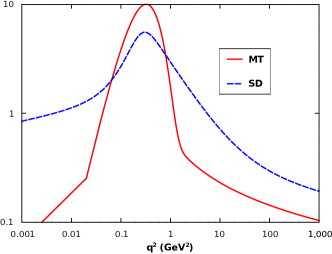
Figure 4: Comparison of the Maris-Tandy (MT) (III.3.1), with $\eta=1.8$, and the soft-divergence (SD) (III.3.2) effective interactions.

III.3.1 Maris-Tandy model

In the Maris-Tandy (MT) model Maris:1997tm ; Maris:1999nt the effective running coupling is given by

$$\alpha_{\textrm{eff}}(q^{2}){}= \pi\eta^{7}\left(\frac{q^{2}}{\Lambda^{2}}\right)^{2}e^{-\eta^{2}\frac{q^{2}}{\Lambda^{2}}}$$

$$+{}\frac{2\pi\gamma_{m}\big{(}1-e^{-q^{2}/\Lambda_{t}^{2}}\big{)}}{\textnormal{ln}[e^{2}-1+(1+q^{2}/\Lambda_{QCD}^{2})^{2}]}\,,$$ (29)

which reproduces the one-loop QCD behavior in the UV and features a Gaussian distribution in the intermediate momentum region (see Fig. 4) that provides dynamical chiral symmetry breaking. The scale $\Lambda_{t}=1$ GeV is introduced for technical reasons and has no impact on the results. Therefore, the interaction strength is characterized by an energy scale $\Lambda$, fixed to $\Lambda=0.74$ GeV to reproduce correctly the pion decay constant from the RL-truncated meson-BSE. The dimensionless parameter $\eta$ controls the width of the interaction. For the anomalous dimension we use $\gamma_{m}=12/(11N_{C}-2N_{f})=12/25$, corresponding to $N_{f}=4$ flavors and $N_{c}=3$ colors. For the QCD scale $\Lambda_{QCD}=0.234$ GeV. Many ground-state hadron observables have been found to be almost insensitive to the value of $\eta$ around $\eta=1.8$ (see, e.g. Krassnigg:2009zh ; Eichmann:2011vu ; Nicmorus:2010mc ). This has been used as an argument in favor of the model independence of Rainbow-Ladder results. Instead of pursuing this line of research, we prefer to introduce a new, non-related model to evaluate the validity of those assertions.

Note that in the numerical resolution of the quark DSE we employ the Pauli-Villars regularization method of the integrals, with a mass scale of $200$ GeV. Moreover, for this model, we fit the quark masses, at the renormalization scale $\mu=19$ GeV, to be $3.7$, $85.2$, $869$ and $3750$ MeV for the $u/d$, $s$, $c$, and $b$ quarks, respectively.

III.3.2 Soft-divergence model

The model of Ref. Alkofer:2008et , called soft-divergence or SD model from here on, is motivated by the desire to account for the $U_{A}(1)$-anomaly by the Kogut-Susskind mechanism Kogut:1973ab ; vonSmekal:1997dq . The effective coupling is constructed as the product of the gluon dressing Alkofer:2003jk ; Alkofer:2003jj and a model for the non-perturbative behavior of the quark-gluon vertex Alkofer:2008tt ,

$$\alpha_{\textrm{eff}}(q^{2}){}= \mathcal{C}\left(\frac{x}{1+x}\right)^{2\kappa}\left(\frac{y}{1+y}\right)^{-\kappa-1/2}$$

$$\times{}\left(\frac{\alpha_{0}+a_{UV}\,x}{1+x}\right)^{-\gamma_{0}}\left(\lambda+\frac{a_{UV}\,x}{1+x}\right)^{-2\delta_{0}}\,\,.$$ (30)

The four terms in parentheses are: the IR scaling of the gluon propagator; IR scaling of the quark-gluon vertex; logarithmic running of the gluon propagator; and the logarithmic running of the quark-gluon vertex. Additionally, the last two are constructed to interpolate between the IR and UV behavior. The remaining terms are defined as

$$\lambda=\frac{\lambda_{S}}{1+y}+\frac{\lambda_{B}\,y}{1+(y-1)^{2}}\,,\quad a_{UV}=\pi\gamma_{m}\left(\frac{1}{\ln{z}}-\frac{1}{z-1}\right),\quad$$ (31)

where

$$x =q^{2}/\Lambda_{YM}^{2}\,,$$ (32)

$$y =q^{2}/\Lambda_{IR}^{2}\,,$$ (33)

$$z =q^{2}/\Lambda_{MOM}^{2}\,,$$ (34)

and $\alpha_{0}=8.915/N_{C}$. Here, $\Lambda_{YM}=0.71$ GeV is the dynamically generated Yang-Mills scale, while $\Lambda_{MOM}\simeq 0.5$ GeV corresponds to the one-loop perturbative running. The IR scaling exponent is $\kappa=0.595353$, and the one-loop anomalous dimensions are related via $1+\gamma_{0}=-2\delta_{0}=\frac{3}{8}\,N_{C}\,\gamma_{m}$, with $\gamma_{m}=12/(11N_{C}-2N_{f})$. We choose $N_{f}=5$ active quark flavors at the renormalization point $\mu=19$ GeV. The constant $\mathcal{C}=0.968$ is chosen such that $\alpha_{\textrm{eff}}$ runs appropriately in the UV. Finally, $\Lambda_{IR}=0.42$ GeV, $\lambda_{S}=6.25$, and $\lambda_{B}=21.83$ determine the IR properties of the quark-gluon vertex and are fitted such that the properties of $\pi$, $K$ and $\rho$ mesons are all reasonably well reproduced. The quark masses at $\mu=19$ GeV are $2.76$, $55.3$, $688$ and $3410$ MeV for the $u/d$, $s$, $c$, and $b$ quarks, respectively.

III.3.3 A remark on missing mesonic effects

The MT and SD model both rely upon the phenomenology of dynamical chiral symmetry breaking in the light quark sector to determine their parameters. Therefore effects we might consider to be beyond RL are absorbed into the model parameterisation. In particular, since these are determined in the light-quark sector we implicitly include those contributions due to interactions at the hadronic level. Here the pion as the lightest hadron plays a special role in the dressing of baryons. Amongst these contributions, non-perturbative pionic effects – also sometimes called pion-cloud effects, see e.g. Ref. Thomas:2007bc and references therein – are expected to have a sizeable influence on hadron properties like the masses or the decay constants. Consequently when fixing the model parameters in the light-quark sector, large parts of these so-called pion-cloud contributions are “parameterised” in cf., the discussion in Ref. Eichmann:2008ae . According to Zweig’s rule the meson-cloud around the triple-strange $\Omega$ will be mostly constituted of kaons. Due to their higher mass as compared to pions, perturbative as well as non-perturbative mesonic effects are significantly smaller for the ground state properties of the $\Omega$ than for the ground state properties of the $\Delta$. However, as we do not change the parameters of the model for the $\Omega$ we expect to find larger deviations from experimental values. This is because we actually then overestimate the beyond RL effects; they look larger despite being actually smaller. This should be kept in mind when comparing our results to lattice data and experimental observations.

IV Results

We computed the electromagnetic current of the Delta and the Omega baryons and extracted the corresponding form factors using (50). As explained in previous sections, the interaction parameters and bare quark masses are fitted to reproduce meson properties. In the baryon sector, therefore, there are no further parameters to be fixed.

Of the four $\Delta(1232)$ isospin partners, we restrict the discussion to the $\Delta^{+}$ since, due to the assumption of isospin symmetry, the form factors of the remaining iso-partners can be obtained by multiplying with the corresponding baryon charge. This, in particular, implies that all $\Delta^{0}$ form factors are identically zero in our approach.

The solution of the Faddeev equation, (III.1), and the subsequent calculation of the electromagnetic current via (III.2) is a numerically complicated task, chiefly as a consequence of the expansion of the Faddeev amplitudes in 128 Lorentz covariants and in a number of Chebyshev polynomials for the angular dependence, which entails that one must solve for an equal number of coefficients. Due to CPU-time and memory limitations, the number of quadrature points used in the numerical integrations must be kept small. Moreover, the presence of inverse powers of $Q$ in the equations for the extraction of the form factors (50) implies that, to obtain reliable results at low $Q$ and even finite results in the limit $Q\rightarrow 0$, very delicate cancelations among the many terms that contribute to the current must take place. For these reasons, that limit is difficult to reach with our current resources, especially for the electric quadrupole, see also Ref. SanchisAlepuz:2012ej , and magnetic octupole form factors.

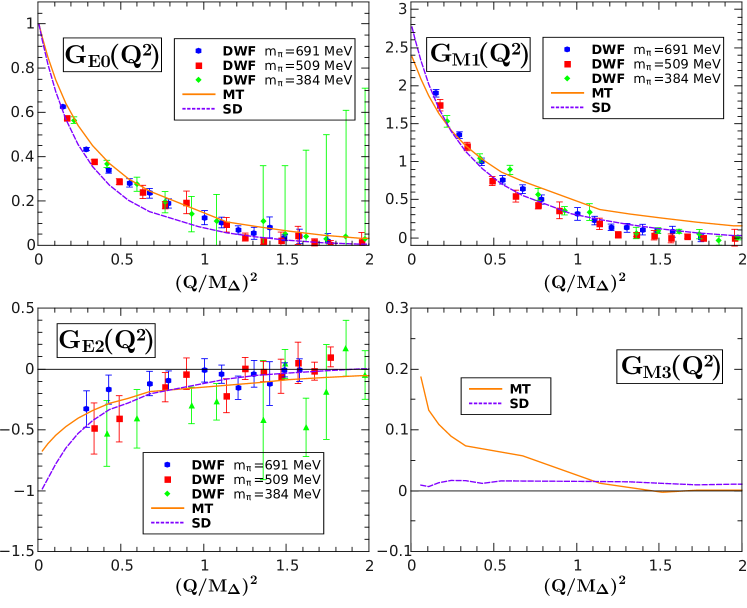
Figure 5: Electromagnetic form factors for the $\Delta^{+}$ using the Maris-tandy (MT) and the soft-divergence (SD) models. We compare with unquenched lattice data (DWF) at three different pion masses Alexandrou:2009hs ; Alexandrou:2009nj

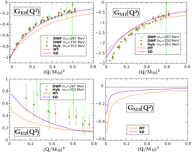
Figure 6: Electromagnetic form factors for the $\Omega^{-}$ using the Maris-tandy (MT) and the soft-divergence (SD) models. We compare with unquenched (DWF) and mixed (Hyb.) lattice data at three different pion masses Alexandrou:2010jv

IV.1 Electric monopole form factor and charge radius

The calculated electric monopole form factor $G_{E0}(Q^{2})$ for the $\Delta^{+}$ is shown in the upper-left panel of Fig. 5 and compared to lattice calculations using dynamical Wilson fermions at three different pion masses Alexandrou:2009hs ; Alexandrou:2009nj . The natural scale associated to the problem is the Delta mass; since MT and SD models, as well as lattice calculations, give different values for this mass, we plot the evolution of the form factors in terms of the dimensionless quantity $Q^{2}/M^{2}$ to remove the scale ambiguity that appears in the comparison of results using different approaches/models. We stress again that, since we assume isospin symmetry, the form factors for the $\Delta^{++}$, $\Delta^{0}$ and $\Delta^{-}$ are obtained by multiplying the former by the corresponding charge.

We see from Fig. 5 that both the MT and the SD models show good agreement with lattice calculations. The $Q^{2}$-evolution of $G_{E0}$ differs slightly for the two models we considered. However, one must bear in mind that we are working here with the simplest chiral-symmetry-preserving interaction kernel (namely, the RL kernel). Since the effective couplings are tailored to reproduce meson observables, we consider it sufficient if they reproduce baryon properties at the level of a few percent. From this point of view, we can say that the behavior of $G_{E0}(Q^{2})$ is qualitatively model independent in our approach.

The charge radius is calculated using the equation

$$<r_{E0}^{2}>=-\frac{6}{G_{E0}(0)}\frac{dG_{E0}(Q^{2})}{dQ^{2}}$$ (35)

and the results are shown in Table 1 for the MT and SD models as well as for lattice calculations. As before, we can suppress the scale dependence of the charge radius by calculating the dimensionless quantity $<r_{E0}^{2}>M_{\Delta}^{2}$. This quantity shows a better agreement with the lattice data than the dimensionful charge radius does, although the value for the SD model is significantly larger.

It is worth mentioning that chiral perturbation theory shows that, when the $\Delta\to N\pi$ decay channel opens, the charge radius changes abruptly to a lower value Ledwig:2011cx . Since in our calculation we do not provide a mechanism for the Delta to decay, it is therefore reasonable that in a full calculation this would lead to a lower result for ${<r_{E0}^{2}>}$. This effect, nevertheless, would be compensated partly by the inclusion of mesonic effects.

	F-MT	F-SD	DW1	DW2	DW3	Exp.
$M_{\Delta}(\textnormal{GeV})$	1.22	1.22	1.395 (18)	1.559 (19)	1.687 (15)	1.232 (2)
$<r_{E0}^{2}>(\textnormal{fm}^{2})$	0.50	0.61	0.373 (21)	0.353 (12)	0.279 (6)
$<r_{E0}^{2}>M_{\Delta}^{2}$	0.75	0.91	0.726 (36)	0.858 (25)	0.794 (14)
$G_{M1}(0)$	2.38	2.77	2.35 (16)	2.68 (13)	2.589 (78)	3.54${}^{+4.59}_{-4.72}$

Table 1: Comparison of results for the $\Delta^{+}$ mass, charge radius $<r_{E0}^{2}>$ and for $G_{M1}(0)~{}~{}(\propto\mu)$. We compare our results for the MT model (F-MT) and for the SD model (F-SD) with a lattice calculation with dynamical Wilson fermions at $m_{\pi}=384$ MeV (DW1), $m_{\pi}=509$ MeV (DW2) and $m_{\pi}=691$ MeV (DW3) Alexandrou:2009hs ; Alexandrou:2009nj . For $G_{M1}(0)$ we also compare with the experimental value Kotulla:2002cg ; Beringer:1900zz .

Since we asume isospin symmetry, in our framework the $\Omega$ baryon is identical to the $\Delta$ but evaluated at a different current-quark mass. We show the evolution of the electromagnetic form factors for the $\Omega^{-}$ in Fig. 6. The calculation shows good agreement with lattice data for both models and, as before, a qualitative agreement between them. The electric charge radius is shown in Table 2. In this case the calculated charge radius is smaller than the lattice values. However, the dimensionless quantity $<r_{E0}^{2}>M_{\Omega}^{2}$ shows good agreement between our results and lattice. Also, our result for this quantity shows little quark-mass dependence, as can be seen by comparing the values for the $\Omega$ and the $\Delta$; presumably, the inclusion of pion-cloud effects, or indeed other flavor dependent contributions beyond that of Rainbow-Ladder, would account for the quark-mass dependence of the charge radius.

	F-MT	F-SD	DW1	DW2	Hyb.	Exp.
$M_{\Omega}(\textnormal{GeV})$	1.65	1.80	1.76 (2)	1.77 (3)	1.78 (3)	1.672
$<r_{E0}^{2}>(\textnormal{fm}^{2})$	0.27	0.27	0.355 (14)	0.353 (8)	0.338 (9)
$<r_{E0}^{2}>M_{\Omega}^{2}$	0.74	0.89	0.726 (36)	0.858 (25)	0.794 (14)
$G_{M1}(0)$	-2.41	-2.71	-3.443 (173)	-3.601 (109)	-3.368 (80)	-3.52 (9)

Table 2: Comparison of results for the $\Omega^{-}$ mass, charge radius $<r_{E0}^{2}>$ and for $G_{M1}(0)~{}~{}(\propto\mu)$. We compare our results for the MT model (F-MT) and for the SD model (F-SD) with a lattice calculation with dynamical Wilson fermions at $m_{\pi}=297$ MeV (DW1), $m_{\pi}=330$ MeV (DW2) and with a hybrid action at $m_{\pi}=353$ MeV (Hyb) Alexandrou:2010jv . For $G_{M1}(0)$ we also compare to the experimental value Beringer:1900zz .

IV.2 Magnetic dipole form factor

As already mentioned above, the magnetic moments of the $\Delta^{+}$ and $\Delta^{++}$ are two of the few electromagnetic properties of the Delta for which we have experimental input. The value at $Q^{2}=0$ of the magnetic dipole form factor $G_{M1}(0)$ for the $\Delta^{+}$, which is related to the magnetic moment via the relation

$$\mu_{\Delta}=\frac{e}{2M_{\Delta}}G_{M1}(0)\,\,,$$ (36)

is given in Table 1. We find good agreement between our results and the lattice data at different pion masses. The value of $G_{M1}(0)$ for the $\Omega^{-}$ is shown in Table 2. Here the comparison with lattice is less favorable, and we clearly underestimate the experimental value which, in this case, is very accurately measured. This is a signature of missing meson-cloud effects whose relevance is, as discussed in the last section, somewhat obscured at the $u/d$ quark mass region since the effective interactions are fitted for that sector, thus in a sense incorporating pion-cloud effects in the parameters of the model.

The evolution of $G_{M1}$ with the photon momentum also compares favorably with lattice results in the case of the $\Delta$. Again, this is not the case for the $\Omega$ as now both models differ significantly from lattice calculations at low-$Q^{2}$, where pion- and kaon-cloud effects are expected to be more relevant.

IV.3 Electric quadrupole form factor

A non-vanishing value for the electric quadrupole moment signals the deformation of the electric charge distribution from sphericity. It would be identically zero if the baryon were formed only by s-wave components. In our approach, the presence of higher angular-momentum components is a natural consequence of requiring Poincaré covariance SanchisAlepuz:2011jn . Nevertheless, the relative importance of these components is dictated by the dynamics and we could still obtain a non-trivial vanishing value for this moment.

We show our calculations for the electric quadrupole form factor and its evolution with $Q^{2}$ in the bottom-right panel of Fig. 5. Although the precise vale of $G_{E2}(0)$ is very sensitive to numerical accuracy (due to the presence of an $1/Q^{4}$ factor when extracting the form factor from the electromagnetic current; see (50)), we clearly see that for both the MT and SD models it is non-vanishing and negative. In the Breit frame (and for positively charged baryons), a negative value of the electric quadrupole moment can be interpreted as an oblate distribution of electric charge. This result agrees with lattice estimations, albeit in this case lattice gives very noisy results and only for relatively high $Q$-values.

As expected, we obtain similar results for the $\Omega^{-}$, although with a different sign coming from the $\Omega$ charge. The electric quadrupole form factor is non-vanishing and negative, and therefore the charge distribution in this case also features an oblate shape. This result agrees as well with the available lattice data.

IV.4 Magnetic octupole form factor

Similar to the electric quadrupole moment, in the Breit frame the magnetic octupole moment measures the deviation from sphericity of the magnetic dipole distribution.

In the case of the magnetic octupole, we have to face an $1/Q^{6}$ factor when extracting the form factor from the electromagnetic current. This entails that, with our current accuracy, we cannot give a reliable value for $G_{M3}(0)$, as is clearly seen in the bottom-right panels of Figs. 5 and 6. However, in both cases and for both the MT and the SD models, we can unambiguously say that the magnetic octupole moment is non-vanishing but small, and positive (negative for the $\Omega^{-}$). We therefore predict a prolate distribution of the magnetic dipole. Unfortunately, for the magnetic octupole form factor there are no reliable lattice calculations to compare with, although a quenched calculation Boinepalli:2009sq suggests a negative sign for the $\Delta^{+}$, in contradiction to our findings. It is very well possible that a more elaborate truncation would change the sign of our results. However, it is for us very difficult to estimate a priori how the inclusion of, for instance, a pion-, resp., kaon-cloud would modify them.

V Summary

We have shown the calculation of the electromagnetic form factors of the $\Delta$ and $\Omega$ baryons in the Poincaré-covariant BSE and DSE framework. This framework has as a goal to provide an unified and systematically improvable approach to hadron physics from continuum QCD. The calculation presented here uses the Rainbow-Ladder truncation of the complete interaction kernel and within this truncation scheme we solved self-consistently for all the elements in the equations, namely the full quark propagator and quark-photon vertex. We have performed the calculations using two different models for the dressings required in the RL truncation, as an attempt to provide results which are qualitatively model-independent.

Our results at $u/d$ quark mass show good agreement with lattice calculations and are compatible with the few experimental data available for the $\Delta$. We obtain a negative value of the electric quadrupole moment, indicating an oblate charge distribution. The sign of the magnetic octupole moment is, however, positive, which would correspond to a prolate magnetic dipole distribution. In the absence of a proper treatment of the current-quark mass dependence of mesonic effects or the quark-gluon interaction in our calculations, we find a weak dependence of the electromagnetic properties on the current-quark mass. It is, therefore, reasonable that we observe discrepancies between our results and lattice calculations for the $\Omega$ form factors.

This calculation, and especially the magnetic octupole form factor, is very sensitive to numerical artefacts and for this reason the inaccuracy of the results is sometimes significant. Improvements on our algorithms and the employment of more elaborate interaction kernels are thus desirable in order to verify, in particular, the sign of the magnetic octupole moment.

Appendix A Extraction of the form factors

In Section II we derived an expression for the electromagnetic current in terms of the photon interaction with the quarks forming a baryon. On the other hand, the form of the current is constrained by Lorentz invariance and current conservation to be a linear combination of a finite numbers of Lorentz covariants with scalar coefficients. These coefficients are the form factors.

The electromagnetic current for a spin-$\nicefrac{{3}}{{2}}$ particle is characterized by four form factors $F_{i}(Q^{2})$ Nozawa:1990gt ; Nicmorus:2010sd . Its expression reads

$$J^{\mu,\alpha\beta}(P,Q)={} \mathbb{P}^{\alpha\alpha^{\prime}}(P_{f})\left[\left((F_{1}+F_{2})i\gamma^{\mu}-F_{2}\frac{P^{\mu}}{M}\right)\delta^{\alpha^{\prime}\beta^{\prime}}\right.$$

$$+\left.\left((F_{3}+F_{4})i\gamma^{\mu}-F_{4}\frac{P^{\mu}}{M}\right)\frac{Q^{\alpha^{\prime}}Q^{\beta^{\prime}}}{4M^{2}}\right]$$

$$~{}\hskip 110.96574pt\mathbb{P}^{\beta^{\prime}\beta}(P_{i})$$ (37)

where $\mathbb{P}$ is the Rarita-Schwinger projector

$$\Lambda^{+}(\hat{P})= \frac{1}{2}\left(\mathbb{1}+\ooalign{\hfil/\hfil\crcr$\hat{P}$}\right)~{},$$ (40)

$$\mathbb{P}_{+}^{\mu\nu}(\hat{\textnormal{P}})= ~{}\Lambda_{+}(\hat{\textnormal{P}})\left(T_{P}^{\mu\nu}-\frac{1}{3}\gamma^{\mu}_{T}\gamma^{\nu}_{T}\right)~{},$$ (41)

with $\gamma^{\mu}_{T}=T_{P}^{\mu\nu}\gamma^{\nu}$, $T_{P}^{\mu\nu}$ the transverse projector (8) and the hat denotes a unit vector. $P_{i}$ and $P_{f}$ are the initial and final baryon total momenta, respectively, $Q=P_{f}-P_{i}$ is the photon momentum, $M$ is the baryon mass and $P=(P_{f}+P_{i})/2$. The form factors that are measured experimentally are the electric monopole ($G_{E_{0}}(Q^{2})$), magnetic dipole ($G_{M_{1}}(Q^{2})$), electric quadrupole ($G_{E_{2}}(Q^{2})$) and magnetic octupole ($G_{M_{3}}(Q^{2})$) form factors. They are related to the $F_{i}^{\prime}s$ via Nozawa:1990gt

$$G_{E_{0}} =\left(1+\frac{2\tau}{3}\right)(F_{1}-\tau F_{2})-\frac{\tau}{3}(1+\tau)\,(F_{3}-\tau F_{4})\,,$$ (42)

$$G_{M_{1}} =\left(1+\frac{4\tau}{5}\right)(F_{1}+F_{2})-\frac{2\tau}{5}(1+\tau)\,(F_{3}+F_{4})\,,$$ (43)

$$G_{E_{2}} =(F_{1}-\tau F_{2})-\frac{1}{2}\,(1+\tau)\,(F_{3}-\tau F_{4})\,,$$ (44)

$$G_{M_{3}} =(F_{1}+F_{2})-\frac{1}{2}\,(1+\tau)\,(F_{3}+F_{4})\,,$$ (45)

with $\tau=Q^{2}/4M^{2}$. It is shown in Nozawa:1990gt that if charge and magnetic dipole distribution in the baryon is spherically symmetric then $G_{E_{2}}$ and $G_{M_{3}}$ must vanish, respectively; therefore they measure the deformation of the object. At $Q^{2}=0$ the form factors define the electric charge ($e_{\nicefrac{{3}}{{2}}}$), magnetic dipole moment ($\mu_{\nicefrac{{3}}{{2}}}$), electric quadrupole moment ($\mathcal{Q}_{\nicefrac{{3}}{{2}}}$) and magnetic octupole moment ($\mathcal{O}_{\nicefrac{{3}}{{2}}}$) of a spin-$\nicefrac{{3}}{{2}}$ particle,

$$e_{\nicefrac{{3}}{{2}}} =G_{E_{0}}(0)\,,$$ (46)

$$\mu_{\nicefrac{{3}}{{2}}} =\frac{e}{2M}G_{M_{1}}(0)\,,$$ (47)

$$\mathcal{Q}_{\nicefrac{{3}}{{2}}} =\frac{e}{M^{2}}G_{E_{2}}(0)\,,$$ (48)

$$\mathcal{O}_{\nicefrac{{3}}{{2}}} =\frac{e}{2M^{3}}G_{M_{3}}(0)\,.$$ (49)

Once the electromagnetic current is calculated from (III.2), the form factors can be extracted using the expressions Nicmorus:2010sd

$$G_{E_{0}} =\frac{s_{2}-2s_{1}}{4i\sqrt{1+\tau}}\,,$$ (50)

$$G_{M_{1}} =\frac{9i}{40\,\tau}\left(s_{4}-2s_{3}\right)\,,$$ (51)

$$G_{E_{2}} =\frac{3}{8i\,\tau^{2}\sqrt{1+\tau}}\left[2s_{1}\left(\tau+\frac{3}{2}\right)-\tau s_{2}\right],$$ (52)

$$G_{M_{3}} =\frac{3i}{16\,\tau^{3}}\left[2s_{3}\left(\tau+\frac{5}{4}\right)-\tau s_{4}\right]~{},$$ (53)

where

$$s_{1} =\textnormal{Tr}\left\{J^{\mu,\alpha\beta}\hat{P}^{\mu}\hat{P}^{\alpha}\hat{P}^{\beta}\right\}~{},$$ (54)

$$s_{2} =\textnormal{Tr}\left\{J^{\mu,\alpha\alpha}\hat{P}^{\mu}\right\}~{},$$ (55)

$$s_{3} =\textnormal{Tr}\left\{J^{\mu,\alpha\beta}\,\gamma^{\mu}_{T}\hat{P}^{\alpha}\hat{P}^{\beta}\right\}~{},$$ (56)

$$s_{4} =\textnormal{Tr}\left\{J^{\mu,\alpha\alpha}\,\gamma^{\mu}_{T}\right\}\,.$$ (57)

References

- (1) B. M. K. Nefkens, M. Arman, H. C. Ballagh, Jr., P. F. Glodis, R. P. Haddock, K. C. Leung, D. E. A. Smith and D. I. Sober, Phys. Rev. D 18 (1978) 3911.
- (2) L. Heller, S. Kumano, J. C. Martinez and E. J. Moniz, Phys. Rev. C 35 (1987) 718.
- (3) R. Wittman, Phys. Rev. C 37 (1988) 2075.
- (4) D. Lin and M. K. Liou, Phys. Rev. C 43 (1991) 930.
- (5) D. H. Lin, M. K. Liou and Z. M. Ding, Phys. Rev. C 44 (1991) 1819.
- (6) A. Bosshard, C. Amsler, J. A. Bistirlich, B. van den Brandt, K. M. Crowe, M. Doebeli, M. Doser and R. P. Haddock et al., Phys. Rev. Lett. 64 (1990) 2619.
- (7) A. Bosshard, C. Amsler, M. Doebeli, M. Doser, M. Schaad, J. Riedlberger, P. Truoel and J. A. Bistirlich et al., Phys. Rev. D 44 (1991) 1962.
- (8) G. Lopez Castro and A. Mariano, Phys. Lett. B 517 (2001) 339 [nucl-th/0006031].
- (9) G. Lopez Castro and A. Mariano, Nucl. Phys. A 697 (2002) 440 [nucl-th/0010045].
- (10) J. Beringer et al. [Particle Data Group Collaboration], Phys. Rev. D 86 (2012) 010001.
- (11) M. Kotulla, J. Ahrens, J. R. M. Annand, R. Beck, G. Caselotti, L. S. Fog, D. Hornidge and S. Janssen et al., Phys. Rev. Lett. 89 (2002) 272001 [nucl-ex/0210040].
- (12) G. Blanpied, M. Blecher, A. Caracappa, R. Deininger, C. Djalali, G. Giordano, K. Hicks and S. Hoblit et al., Phys. Rev. C 64 (2001) 025203.
- (13) C. Alexandrou, T. Korzec, G. Koutsou, C. Lorce, J. W. Negele, V. Pascalutsa, A. Tsapalis and M. Vanderhaeghen, Nucl. Phys. A 825 (2009) 115 [arXiv:0901.3457 [hep-lat]].
- (14) C. Alexandrou, T. Korzec, G. Koutsou, C. Lorce, V. Pascalutsa, M. Vanderhaeghen, J. W. Negele and A. Tsapalis, PoS CD 09 (2009) 092 [arXiv:0910.3315 [hep-lat]].
- (15) C. Alexandrou, T. Korzec, G. Koutsou, J. W. Negele and Y. Proestos, Phys. Rev. D 82 (2010) 034504 [arXiv:1006.0558 [hep-lat]].
- (16) C. Aubin, K. Orginos, V. Pascalutsa and M. Vanderhaeghen, Phys. Rev. D 79 (2009) 051502 [arXiv:0811.2440 [hep-lat]].
- (17) S. Boinepalli, D. B. Leinweber, P. J. Moran, A. G. Williams, J. M. Zanotti and J. B. Zhang, Phys. Rev. D 80 (2009) 054505 [arXiv:0902.4046 [hep-lat]].
- (18) G. Ramalho and M. T. Pena, J. Phys. G G 36 (2009) 085004 [arXiv:0807.2922 [hep-ph]].
- (19) G. Ramalho, M. T. Pena and F. Gross, Phys. Lett. B 678 (2009) 355 [arXiv:0902.4212 [hep-ph]].
- (20) G. Ramalho, M. T. Pena and F. Gross, Phys. Rev. D 81 (2010) 113011 [arXiv:1002.4170 [hep-ph]].
- (21) G. Ramalho and M. T. Pena, Phys. Rev. D 83 (2011) 054011 [arXiv:1012.2168 [hep-ph]].
- (22) T. Ledwig, A. Silva and M. Vanderhaeghen, Phys. Rev. D 79 (2009) 094025 [arXiv:0811.3086 [hep-ph]].
- (23) L. S. Geng, J. Martin Camalich and M. J. Vicente Vacas, Phys. Rev. D 80 (2009) 034027 [arXiv:0907.0631 [hep-ph]].
- (24) T. Ledwig, J. Martin-Camalich, V. Pascalutsa and M. Vanderhaeghen, Phys. Rev. D 85 (2012) 034013 [arXiv:1108.2523 [hep-ph]].
- (25) K. Azizi, Eur. Phys. J. C 61 (2009) 311 [arXiv:0811.2670 [hep-ph]].
- (26) H. Sanchis-Alepuz, R. Alkofer, G. Eichmann and S. Villalba-Chavez, PoS LC 2010 (2010) 018 [arXiv:1010.6183 [hep-ph]].
- (27) H. Sanchis-Alepuz, G. Eichmann, S. Villalba-Chavez and R. Alkofer, Phys. Rev. D 84 (2011) 096003 [arXiv:1109.0199 [hep-ph]].
- (28) H. Sanchis-Alepuz, arXiv:1206.5190 [hep-ph].
- (29) H. Haberzettl, Phys. Rev. C 56 (1997) 2041 [nucl-th/9704057].
- (30) A. N. Kvinikhidze and B. Blankleider, Phys. Rev. C 60 (1999) 044003 [nucl-th/9901001].
- (31) A. N. Kvinikhidze and B. Blankleider, Phys. Rev. C 60 (1999) 044004 [nucl-th/9901002].
- (32) M. Oettel, M. Pichowsky and L. von Smekal, Eur. Phys. J. A 8 (2000) 251 [nucl-th/9909082]; M. Oettel, R. Alkofer and L. von Smekal, Eur. Phys. J. A 8 (2000) 553 [nucl-th/0006082].
- (33) H. J. Munczek, Phys. Rev. D 52 (1995) 4736 [hep-th/9411239].
- (34) A. Bender, C. D. Roberts and L. Von Smekal, Phys. Lett. B 380 (1996) 7 [nucl-th/9602012].
- (35) P. Maris, C. D. Roberts and P. C. Tandy, Phys. Lett. B 420 (1998) 267 [nucl-th/9707003].
- (36) M. S. Bhagwat and P. Maris, Phys. Rev. C 77 (2008) 025203 [nucl-th/0612069].
- (37) P. Maris and C. D. Roberts, Phys. Rev. C 56 (1997) 3369 [nucl-th/9708029].
- (38) P. Maris and P. C. Tandy, Phys. Rev. C 60 (1999) 055214 [nucl-th/9905056].
- (39) R. Alkofer, C. S. Fischer and R. Williams, Eur. Phys. J. A 38 (2008) 53 [arXiv:0804.3478 [hep-ph]].
- (40) R. Alkofer, C. S. Fischer, F. J. Llanes-Estrada and K. Schwenzer, Annals Phys. 324 (2009) 106 [arXiv:0804.3042 [hep-ph]].
- (41) C. S. Fischer and R. Williams, Phys. Rev. Lett. 103 (2009) 122001 [arXiv:0905.2291 [hep-ph]].
- (42) R. Williams, EPJ Web Conf. 3 (2010) 03005 [arXiv:0912.3494 [hep-ph]].
- (43) L. Chang and C. D. Roberts, Phys. Rev. Lett. 103 (2009) 081601 [arXiv:0903.5461 [nucl-th]].
- (44) C. S. Fischer, D. Nickel and J. Wambach, Phys. Rev. D 76 (2007) 094009 [arXiv:0705.4407 [hep-ph]].
- (45) C. S. Fischer and R. Williams, Phys. Rev. D 78 (2008) 074006 [arXiv:0808.3372 [hep-ph]].
- (46) H. Sanchis-Alepuz, R. Alkofer, G. Eichmann and R. Williams, PoS QCD-TNT-II (2011) 041 [arXiv:1112.3214 [hep-ph]].
- (47) A. Krassnigg, Phys. Rev. D 80 (2009) 114010 [arXiv:0909.4016 [hep-ph]].
- (48) G. Eichmann, Phys. Rev. D 84 (2011) 014014 [arXiv:1104.4505 [hep-ph]].
- (49) D. Nicmorus, G. Eichmann, A. Krassnigg and R. Alkofer, Few Body Syst. 49 (2011) 255 [arXiv:1008.4149 [hep-ph]].
- (50) J. B. Kogut and L. Susskind, Phys. Rev. D 10 (1974) 3468.
- (51) L. von Smekal, A. Mecke and R. Alkofer, In *Big Sky 1997, Intersections between particle and nuclear physics* 746-749 [hep-ph/9707210].
- (52) R. Alkofer, W. Detmold, C. S. Fischer and P. Maris, Nucl. Phys. Proc. Suppl. 141 (2005) 122 [hep-ph/0309078].
- (53) R. Alkofer, W. Detmold, C. S. Fischer and P. Maris, Phys. Rev. D 70 (2004) 014014 [hep-ph/0309077].
- (54) A. W. Thomas, Prog. Theor. Phys. 168 (2007) 614 [arXiv:0711.2259 [nucl-th]].
- (55) G. Eichmann et al., Phys. Rev. C 77 (2008) 042202 [arXiv:0802.1948 [nucl-th]].
- (56) H. Sanchis-Alepuz, R. Alkofer and R. Williams, PoS QNP 2012 (2012) 112 [arXiv:1206.6599 [hep-ph]]; PoS Confinement X (2013) 101.
- (57) S. Nozawa and D. B. Leinweber, Phys. Rev. D 42 (1990) 3567.
- (58) D. Nicmorus, G. Eichmann and R. Alkofer, Phys. Rev. D 82 (2010) 114017 [arXiv:1008.3184 [hep-ph]].