Threshold-Coloring and Unit-Cube Contact Representation of Graphs

Abstract

In this paper we study threshold coloring of graphs, where the vertex colors represented by integers are used to describe any spanning subgraph of the given graph as follows. Pairs of vertices with near colors imply the edge between them is present and pairs of vertices with far colors imply the edge is absent. Not all planar graphs are threshold-colorable, but several subclasses, such as trees, some planar grids, and planar graphs without short cycles can always be threshold-colored. Using these results we obtain unit-cube contact representation of several subclasses of planar graphs. Variants of the threshold coloring problem are related to well-known graph coloring and other graph-theoretic problems. Using these relations we show the NP-completeness for two of these variants, and describe a polynomial-time algorithm for another.

1 Introduction

Graph coloring is among the fundamental problems in graph theory. Typical applications of the problem and its generalizations are in job scheduling, channel assignments in wireless networks, register allocation in compiler optimization and many others [15]. In this paper we consider a new graph coloring problem in which we assign colors (integers) to the vertices of a graph $G$ in order to define a spanning subgraph $H$ of $G$. In particular, we color the vertices of $G$ so that for each edge of $H$, the two endpoints are near, i.e., their distance is within a given “threshold”, and for each edge of $G\setminus H$, the endpoints are far, i.e., their distance greater than the threshold; see Fig 1.

The motivation of the problem is twofold. First, such coloring can be used for the Frequency Assignment Problem [10], which asks for assigning frequencies to transmitters in radio networks so that only specified pairs of transmitters can communicate with each other. Second, such coloring can be used in the context of the geometric problem of unit-cube contact representation of planar graphs. In such a representation of a graph, each vertex is represented by a unit-size cube and each edge is realized by a common boundary with non-zero area between the two corresponding cubes. Finding classes of planar graphs with unit-cube contact representation was recently posed as an open question by Bremner et al. [2]. In this paper we partially address this problem as an application of our coloring problem in the following way. Suppose a planar graph $G$ has a unit-cube contact representation where one face of each cube is co-planar; see Fig. 1(a). Assume that we can define a spanning subgraph $H$ of $G$ by our particular vertex coloring. We show that it is possible to compute a unit-cube contact representation of $H$ by lifting the cube for each vertex $v$ by the amount equal to the color of $v$ (where the size or side-length of the cubes are roughly equal to the threshold); see Fig. 1(b).

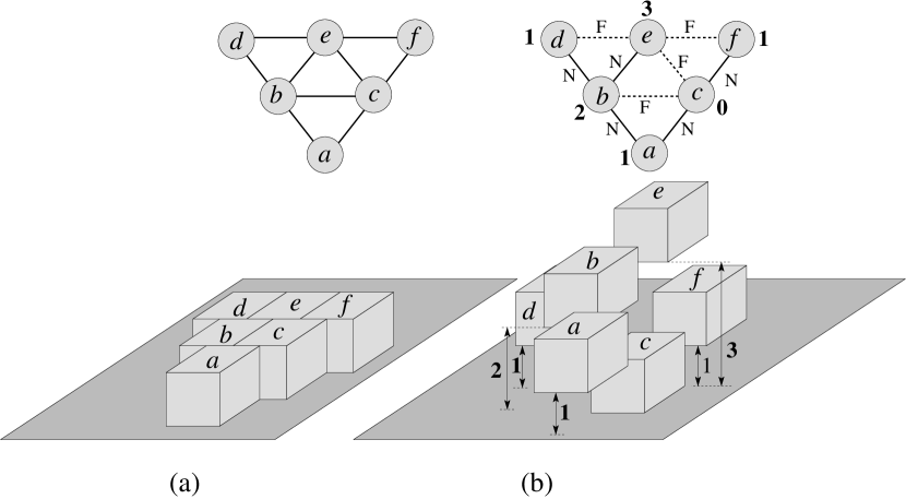
Figure 1: (a) A planar graph $G$ and its unit-cube contact representation where the bottom faces of all cubes are co-planar, (b) a spanning subgraph $H$ of $G$ with a $(4,1)$-threshold-coloring and its unit-cube contact representation. Far edges are shown dashed, near edges are shown solid.

1.1 Problem Definition

An edge-labeling of graph $G=(V,E)$ is a mapping $\ell:E\rightarrow\{N,F\}$ assigning labels $N$ or $F$ to each edge of the graph; we informally name edges labeled with $N$ as the near edges, and edges labeled with $F$ as the far edges. Note that such an edge labeling of $G$ defines a partition of the edges $E$ into near and far edges. By abuse of notation the pair $\{N,F\}$ also denotes this partition.

Let $r\geq 1$ and $t\geq 0$ be two integers and let $[1\dots r]$ denote a set of $r$ consecutive integers. For a graph $G=(V,E)$ and an edge-labeling $\ell:E\rightarrow\{N,F\}$ of $G$, a $(r,t)$-threshold-coloring of $G$ with respect to $\ell$ is a coloring $c:V\rightarrow[1\dots r]$ such that for each edge $e=(u,v)\in E$, $e\in N$ if and only if $|c(u)-c(v)|\leq t$. We call $r$ and $t$ the range and the threshold. Note that the set of near edges defines a spanning subgraph $H=(V,N)$ of $G$, where $H$ is a spanning subgraph of graph $G$ if it contains all vertices of $G$. $H$ is a threshold subgraph of $G$ if there exists such a threshold-coloring.

A graph $G$ is total-threshold-colorable if for every edge-labeling $\ell$ of $G$ there exists an $(r,t)$-threshold-coloring of $G$ with respect to $\ell$ for some $r\geq 1,t\geq 0$. Informally speaking, for every partition of edges of $G$ into near and far edges, we can produce vertex colors so that endpoints of near edges receive near colors, and endpoints of far edges receive colors that are far apart. A graph $G$ is $(r,t)$-total-threshold-colorable if it is total-threshold-colorable for the range $r$ and threshold $t$. In this paper we focus on the following problem variants:

Problem 1

(Total-Threshold-Coloring Problem) Given a graph $G$, is $G$ total-threshold-colorable, that is, is every spanning subgraph of $G$ a threshold subgraph of $G$?

The problem is closely related to the question about whether a particular spanning graph $H$ of $G$ is threshold-colorable.

Problem 2

(Threshold-Coloring Problem) Given a graph $G$ and a spanning subgraph $H$, is $H$ a threshold subgraph of $G$ for some integers $r\geq 1,t\geq 0$?

Another interesting variant of the threshold-coloring is the one in which we specify that the graph $G$ is the complete graph. In this case we call $H$ an exact-threshold graph if $H$ is a threshold subgraph of the complete graph $G$ for some integers $r\geq 1,t\geq 0$.

Problem 3

(Exact-Threshold-Coloring Problem) Given a graph $H$, is $H$ an exact-threshold graph?

In the final variant of the problem we assume that the threshold and the range are the part of the input:

Problem 4

(Fixed-Threshold-Coloring Problem) Given a graph $G$, a spanning subgraph $H$, and integers $r\geq 1,t\geq 0$, is $H$ $(r,t)$-threshold-colorable?

1.2 Related Work

Many problems in graph theory deal with coloring or assigning labels to the vertices of a graph; many graph classes are defined based on such coloring and labeling; see [1] for an excellent survey. To the best of our knowledge, total-threshold-colorability defines a new class of graphs. Here we mention two closely related classes: threshold graphs and difference graphs. Threshold graphs are ones for which there is a real number $S$ and for every vertex $v$ there is a real weight $a_{v}$ such that $(v,w)$ is an edge if and only if $a_{v}+a_{w}\geq S$ [14]. A graph is a difference graph if there is a real number $S$ and for every vertex $v$ there is a real weight $a_{v}$ such that $|a_{v}|<S$ and $(v,w)$ is an edge if and only if $|a_{v}-a_{w}|\geq S$ [11]. Note that for both classes the threshold (real number $S$) defines edges between all pairs of vertices, while in our setting the threshold defines only the edges of a graph $G$, which is not necessarily a complete graph. Both threshold and difference graphs can be characterized in terms of forbidden induced subgraphs. For our problem such a characterization is unknown. For details on threshold and difference graphs, see [14].

Another related graph coloring problem is the distance constrained graph labeling. Here the goal is to find $L(p_{1},\dots,p_{k})$-labeling of the vertices of a graph so that for every pair of vertices at distance at most $i\leq k$ we have that the difference of their labels is at least $p_{i}$. The most studied variant is $L(2,1)$-labeling [9, 6]. In [9] it was shown that minimizing the number of labels in $L(2,1)$-labeling is NP-complete, even for graphs with diameter 2. Further, it shown that it is also NP-complete to determine whether a labeling exists with at most $k$ labels for every fixed integer $k\geq 4$ [5].

A threshold-coloring of a planar graph can be used to find a contact representation of the graph with cuboids (axis aligned boxes) in 3D. Thomassen [16] shows that any planar graph has a proper contact representation by cuboids in 3D. In a contact representation of a graph, the vertices are represented by cuboids (or other polygonal shapes) and the edges are realized by a common boundary of the two corresponding cuboids. A contact representation is proper if for each edge the corresponding common boundary has non-zero area. Felsner and Francis [4] prove that any planar graph has a (non-proper) contact representation by cubes.

Bremner et al. [2] proves that the same result does not hold when using only unit cubes. Our results on threshold-coloring of planar graphs translates to results on classes of planar graphs that can be represented by contact of unit cubes.

1.3 Our Contribution

1. We study the Total-Threshold-Coloring Problem for various subclasses of planar graphs. In particular, we show that several subclasses of planar graphs are threshold-colorable (e.g., trees, hexagonal grids, planar graphs without any cycles of length $\leq 9$) and several subclasses are not (e.g., triangular grid, 4-3 grid). Our results are summarized in Table 1.

   graph classes	Cycle	Tree	Fan	Triangular Grid	Square Grid	Hexagonal Grid	Octagonal-Square Grid	Square-Triangle Grid	Planar Graph w/o Cycles of size $\leq 9$
   threshold coloring	$r=5$, $t=1$	$r=2$, $t=0$	$r=5$, $t=1$	No	Open	$r=5$, $t=1$	$r=5$, $t=1$	No	$r=8$, $t=2$
   unit-cube contact	Yes	No	No	Open	Yes	Yes	Yes	Open	No

   Table 1: Results on the Total-Threshold-Coloring Problem. “No” entries in the last row follow from the fact that graphs with vertices of high degrees cannot have unit-cube representation [2].

2. As an application of the threshold-coloring problem, we address the problem of contact representation of planar graphs with unit cubes. Given a planar graph, we investigate whether each of its subgraphs has a contact representation with unit cubes. We show how we can use the threshold-coloring for computing unit-cube contact representations for some subclasses of planar graphs. For some other subclasses, we gave algorithms to directly compute unit-cube contact representation without using threshold-coloring. Thus we answer some of the open problems from [2] for some subclasses of planar graphs. The last column of Table 1 summarizes these results.

3. Finally we study the relation of the various threshold-coloring problems with other graph-theoretic problems. Specifically, we show that the Threshold-Coloring Problem and the Fixed-Threshold-Coloring Problem are NP-complete by reductions from a graph sandwich problem and the classical vertex coloring problem, respectively. We also show that the Exact-Threshold-Coloring Problem can be solved in linear time since it is equivalent to the proper interval graph recognition problem.

2 Threshold-Coloring and Other Graph Problems

We begin by showing the connections between threshold-colorability and some classical graph-theoretical and graph coloring problems.

2.1 Vertex Coloring Problem

Let $G=(V,E)$ be a graph. We call $G$ $k$-vertex-colorable if there exists a coloring $c:V\rightarrow[1\dots k]$ such that for any edge $(u,v)\in E$, $c(u)\neq c(v)$, that is, $u$ and $v$ have different colors. Given an input graph $G$ and an integer $k>0$, the vertex coloring problem asks whether there exists a $k$-vertex-coloring of $G$.

Lemma 1

Let $G=(V,E)$ be a graph and let $k$ be a positive integer. Define an edge-labeling $\ell:E\rightarrow\{N,F\}$ that assigns each edge the label $F$, that is, for each edge $e\in E$, $\ell(e)=F$. Then $G$ has a $k$-vertex-coloring if and only if there exists a $(k,0)$-threshold-coloring of $G$ with respect to $\ell$.

Proof

Let $c:V\rightarrow[1\dots k]$ define a mapping of the vertices of $G$ to the colors $[1\dots k]$. Then $c$ is a $k$-vertex-coloring of $G$ $\Leftrightarrow$ for each edge $e=(u,v)\in E$, $c(u)\neq c(v)$ $\Leftrightarrow$ for each edge $e=(u,v)\in E$, $|c(u)-c(v)|>0$ $\Leftrightarrow$ $c$ is a $(k,0)$-threshold-coloring of $G$ with respect to $\ell$.

Corollary 1

The Fixed-Threshold-Coloring Problem is NP-complete.

2.2 Proper Interval Representation Problem

An interval representation [1] for a graph $G=(V,E)$ is one where each vertex $v$ of $G$ is represented by an interval $I(v)$ of $\mathbb{R}$ such that for any edge $(u,v)\in E$, the intervals $I(u)$ and $I(v)$ have a non-empty intersection, that is, $I(u)\cap I(v)\neq\emptyset$. A proper interval representation [1] for $G$ is an interval representation of $G$ where no interval properly contains another. A proper interval graph is one that has a proper interval representation. Equivalently, a proper interval graph is one that has an interval representation with unit intervals. The problem of proper interval representation for a graph $G$ asks whether $G$ has a proper interval representation. The problem has been studied extensively [3, 12], and it still attracts attention [13].

Lemma 2

A graph is an exact-threshold graph if and only if it is a proper interval graph.

Proof

Let graph $H=(V,E)$ be an exact-threshold graph. This implies that there are integers $r\geq 1,t\geq 0$ and a mapping $c:V\rightarrow[1\dots r]$ such that for any pair $u,v\in V$, $(u,v)\in E\Leftrightarrow|c(u)-c(v)|\leq t$ $\Leftrightarrow|c(u)-c(v)|<t+\epsilon$ with $0<\epsilon<1$ since $c(u)$ and $c(v)$ are integers. We can find an interval representation of $H$ with unit intervals as follows. Choose an arbitrary $\epsilon$ such that $0<\epsilon<1$. Define for each vertex $v$ of $H$ an interval $I(v)$ of unit length where the left-end has $x$-coordinate $c(v)/(t+\epsilon)$. Then for any two vertices $u$ and $v$ of $H$, $I(u)$ and $I(v)$ has a non-empty intersection if and only if $|\frac{c(u)}{t+\epsilon}-\frac{c(v)}{t+\epsilon}|\leq 1$ $\Leftrightarrow|c(u)-c(v)|\leq(t+\epsilon)\Leftrightarrow|c(u)-c(v)|\leq t$ since $c(u)$ and $c(v)$ are integers. Then $l(u)$ and $l(v)$ has non-empty intersection if and only if $(u,v)$ is an edge of $H$. Thus these intervals yield an interval representation of $H$.

Conversely, if $H$ has an interval representation $\Gamma$ with unit intervals, we can find an exact $(r,t)$-threshold-coloring of $H$ for some integers $r\geq 1,t\geq 0$. Scale $\Gamma$ by a sufficiently large factor $t$ such that each end-point of some interval in $\Gamma$ has a positive integer $x$-coordinate (after possible translation in the positive $x$ direction). Let $r$ be the $x$-coordinate of the right end-point of the rightmost interval in this scaled representation. Define a coloring $c:V\rightarrow[1\dots r]$ where for each vertex $v$ of $H$, $c(v)$ equals the $x$-coordinate of the left end-point of the interval for $v$. Also define the threshold as the scaling factor $t$. It is easy to verify that $c$ is indeed an $(r,t)$-threshold-coloring.

Since recognition of proper interval graphs can be done in linear time [12, 3, 13], we have

Corollary 2

The Exact-Threshold-Coloring Problem can be solved in linear time.

2.3 Graph Sandwich Problem

The graph sandwich problem is defined in [8] as follows.

Problem 5

Given two graphs $G_{1}=(V,E_{1})$ and $G_{2}=(V,E_{2})$ on the same vertex set $V$, where $E_{2}\subseteq E_{1}$, and a property $\Pi$, does there exist a graph $H=(V,E)$ on the same vertex set such that $E_{2}\subseteq E\subseteq E_{1}$ and $H$ satisfies property $\Pi$?

Here $E_{1}$ and $E_{2}$ can be thought of as universal and mandatory sets of edges, with $E$ sandwiched between the two sets. We are interested in a particular property for the graph sandwich problem: “proper interval representability”. A graph satisfies proper interval representability if it admits a proper interval representation.

Lemma 3

Let $G=(V,E_{G})$ and $H=(V,E_{H})$ be two graphs on the same vertex set $V$ such that $E_{H}\subseteq E_{G}$. Then the threshold-coloring problem for $G$ with respect to the edge partition $\{E_{H},E_{G}-E_{H}\}$ is equivalent to the graph sandwich problem for the vertex set $V$, mandatory edge set $E_{H}$, universal edge set $E_{H}\cup(V\times V-E_{G})$ and proper interval representability property.

Proof

Let $E_{U}$ denote the universal edge set $E_{H}\cup(V\times V-E_{G})$ for the graph sandwich problem. Suppose there exists a graph $H^{*}=(V,E^{*})$ such that $E_{H}\subseteq E^{*}\subseteq E_{U}$ and $H^{*}$ has a proper interval representation. Then by Lemma 2, there exist two integers $r\geq 0$ and $t\geq 0$ and a coloring $c:V\rightarrow[1\dots r]$ such that for any pair $u,v\in V$, $|c(u)-c(v)|\leq t$ if and only if $(u,v)\in E^{*}$. We now show that $c$ is in fact a desired threshold-coloring for $G$. Consider an edge $e=(u,v)\in E_{G}$. If $e\in E_{H}$ then $e\in E^{*}$ since $E_{H}\subseteq E^{*}$ and hence $|c(u)-c(v)|\leq t$. On the other hand if $e\in(E_{G}-E_{H})$, $e\notin E_{U}=E_{H}\cup(V\times V-E_{G})$ and therefore $e\notin E^{*}$ since $E^{*}\subseteq E_{U}$. Hence $|c(u)-c(v)|>t$.

Conversely, if there exists integers $r\geq 1$ and $t\geq 0$ such that there is an $(r,t)$-threshold-coloring $c:V\rightarrow[1\dots r]$ of $G$ with respect to the edge partition $\{E_{H},E_{G}-E_{H}\}$, then define an edge set $E^{*}$ as follows. For any pair $u,v\in V$, $(u,v)\in E^{*}$ if and only if $|c(u)-c(v)|\leq t$. Clearly the graph $H^{*}=(V,E^{*})$ has an exact $(r,t)$-threshold-coloring and hence by Lemma 2, $H^{*}$ has a proper interval representation. Furthermore for any edge $e=(u,v)\in E_{H}$, $|c(u)-c(v)|\leq t$ and hence $e\in E^{*}$. Thus $E_{H}\subseteq E^{*}$. Again if $e\in E^{*}$ then $|c(u)-c(v)|let$. Therefore either $e\in E_{H}$ or $e\notin E_{G}\Rightarrow e\in(V\times V-E_{G})$. Hence $e\in(E_{H}\cup(V\times V-E_{G}))=E_{U}$. Thus $E^{*}\subseteq E_{U}$. Therefore $E^{*}$ is sandwiched between the mandatory and the universal set of edges and $H^{*}$ has a proper interval representation.

Golumbic et al. [7] proved that the graph sandwich problem is NP-complete for the proper-interval-representability property. Hence we have

Corollary 3

The Threshold-Coloring Problem is NP-complete.

Summarizing the results in this section, we have the following theorem.

Theorem 2.1

The Threshold-Coloring Problem and the Fixed-Threshold-Coloring Problem are NP-complete while the Exact-Threshold-Coloring Problem can be solved in linear time.

3 Total-Threshold-Coloring of Graphs

In this section we address the Total-Threshold-Coloring Problem: is a given graph $G$ total-threshold-colorable, that is, can every spanning subgraph of $G$ be represented by appropriately coloring the vertices of $G$?

First note that not every graph (not even every planar graph) is total-threshold-colorable. Suppose that $G=K_{4}$, and we would like to represent a subgraph where four of the edges remain and span a $4$-cycle, while the other two edges are removed (edge-partitioning $\{N,F\}$). Assume that there exists an $(r,t)$-threshold-coloring with colors $c_{1},c_{2},c_{3},c_{4}$ for vertices $v_{1},v_{2},v_{3},v_{4}$ respectively. Without loss of generality assume $c_{4}$ is the highest color and $(v_{1},v_{4})\in F$, hence also $(v_{2},v_{3})\in F$. Also assume $c_{3}\geq c_{2}$ and consequently $c_{4}-c_{2}\geq c_{3}-c_{2}$. The left side of the inequality should be at most $t$, and the right side strictly greater than $t$, which cannot be accomplished by any choice of the range and the threshold.

Next we investigate several subclasses of planar graphs. For each of them we either give an algorithm to find an $(r,t)$-threshold-coloring of any graph in that class with respect to each edge-partition for some $r\geq 1,t\geq 0$; or we give an example of a graph in that class and the edge-partition for which there is no threshold-coloring.

3.1 Paths, Cycles, Trees, Fans

For paths and trees there is a trivial coloring with threshold $t=0$ and two colors. Choose an arbitrary vertex as the root and color it $0$. Color $1$ all vertices with an odd number of far edges on the shortest path to the root. Color $0$ all vertices with an even number of far edges to the root. Then all vertices connected by a near edge of $G$ get the same color, and vertices connected by a far edge get different colors; see Fig. 2(a).

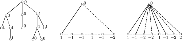
Figure 2: Threshold-coloring of trees, cycles, and fans.

For cycles and fans there is a coloring scheme with threshold $t=1$ and five colors. A fan is obtained from a path $P$ by adding a new vertex $v$ connected to all vertices of the path. We use colors $\{-2,-1,0,1,2\}$ to color a fan. The vertices of $P$ are colored by $-1$ and $1$, and $v$ is colored by $0$. After this initial coloring some of the far edges $(u,v),u\in P$ might have $|c(u)-c(v)|=1$. We fix it by changing the color of $u$ from $1$ to $2$ or from $-1$ to $-2$; see Fig. 2(c). It is easy to see that the same algorithm can be applied to color a cycle; see Fig. 2(b).

3.2 Triangular Grid

In a triangular grid (planar weak dual of a hexagonal grid) all faces are triangles and internal vertices have degree 6. It is easy to show that a triangular grid is not total-threshold-colorable. Consider the graph with vertices $v_{0},v_{1},v_{2},u_{0},u_{1},u_{2}$, where each vertex $u_{i}$ is adjacent to $v_{i+1}$ and $v_{i+2}$ (mod 3); see Fig. 3. Let $F=\{(v_{0},v_{1})$, $(v_{1},v_{2})$, $(v_{2},v_{0})\}$, and let $N$ contain the remaining $6$ edges. Assume that there exists a $(r,t)$-threshold-coloring $c$. Without loss of generality, let $c(v_{0})<c(v_{1})<c(v_{2})$. Now on one hand $c(v_{2})-c(v_{0})>2t$ and on the other $c(v_{2})-c(v_{0})\leq|c(v_{2})-c(u_{1})|+|c(u_{1})-c(v_{0})|\leq 2t$, which is impossible. This also proves that outerplanar graphs are not total-threshold-colorable in general.

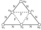
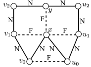
Figure 3: Graphs which are not total-threshold-colorable.

3.3 Hexagonal Grid

In a hexagonal grid all faces are 6-sided and internal vertices have degree 3 (planar weak dual of the triangular grid). Here we show that the hexagonal grid is total-threshold-colorable with $r=5$ and $t=1$. We begin with a simple lemma about (5,1) color space. For convenience, we use colors $\{-2,-1,0,1,2\}$.

Lemma 4

Let $P_{2}=\{v_{0},v_{1},v_{2}\}$ be a path of length 2. Then for any edge-labeling of $P_{2}$ and a fixed color $k\in\{-2,-1,1,2\}$, there is a threshold-coloring $c$ of $P_{2}$ with threshold $t=1$, where $c(v_{0})=0$, $c(v_{2})=k$ and $c(v_{1})\in\{-2,-1,1,2\}$.

Proof

Depending on whether the edge $(v_{0},v_{1})$ is near or far, choose $c(v_{1})$ to be $1$ or $2$. If the label of $(v_{1},v_{2})$ disagrees with the colors of $v_{1}$ and $v_{2}$ then we change the sign of $c(v_{1})$.

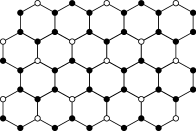
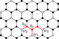
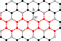
Figure 4: Total-threshold-coloring of the hexagonal grid. (a) White vertices get color 0, black vertices get one of the colors $-2,-1,1,2$. (b) A color assignment to $b_{1}$ can be extended to vertices $w_{2}$ and $w_{3}$ based on the labels of the red dashed edges. (c) The process assigns colors for the red vertices.

Lemma 5

Any hexagonal grid is $(5,1)$-total-threshold-colorable.

Proof

The coloring is done in two steps. In the first step we assign color $0$ for a set of independent vertices of $G$ as shown in Fig. 4, where the colored vertices are white. Note that no two white vertices have a shortest path of length less than $3$.

In the second step we find a coloring of the remaining black vertices, using only four colors $\{-2,-1,1,2\}$. Let $w_{1}$ be a white vertex. We randomly choose one of its black neighbors $b_{1}$, and assign a color for $b_{1}$ based on the label of edge $(w_{1},b_{1})$. Now vertex $b_{1}$ has two white vertices $w_{2}$ and $w_{3}$ within distance $2$. Using Lemma 4 we can (uniquely) extend the coloring of $b_{1}$ to $w_{2}$ (symmetrically, to $w_{3}$) so that additional black vertex $b_{2}$ gets a color. Again, the coloring of $b_{2}$ can be extended to its nearest white neighbor. We continue such a propagation of colors, see Figs. 4 and 4 where processed black vertices and edges are shown dashed red. One can easily see that the process will color a row of hexagons with alternate upper and lower legs.

To complete the coloring of $G$ we choose a white vertex in the next row of hexagons and initiate a similar propagation process. For example, one can use vertices $w$ and $b$ shown in Fig. 4.

3.4 Octagonal-Square Grid

Lemma 6

Any octagonal-square grid is $(5,1)$-total-threshold-colorable.

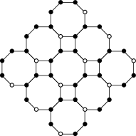
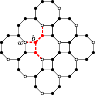
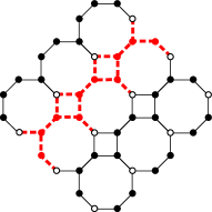
Figure 5: Total-threshold-coloring of the octagonal-square grid.

Proof

We use colors $\{-2,-1,0,1,2\}$ and threshold $t=1$ to find a coloring; the proof is similar to the proof of Lemma 5. We start by partitioning the vertices of the graph into white and black as shown in Fig. 5, and we assign color $0$ to the white ones. Then we choose a white vertex $w$ and its black neighbor $b$ as in Fig. 5, and we assign colors $\{-2,-1,1,2\}$ to the “row” of black vertices. It is easy to see that the coloring of rows can be done independently; see Fig. 5.

3.5 Square-Triangle Grid

We prove that the graph in Fig. 3 is not total-threshold-colorable. Assume to the contrary that $c$ is a $(r,t)$-threshold-coloring. Without loss of generality let $c(v_{0})<c(u_{0})$. Since $(v_{1},u_{0})$ is a far edge and $(v_{0},x),(u_{0},x)$ are near we have $c(v_{0})<c(x)<c(u_{0})$. Similar argument shows that $c(v_{1})<c(v_{0})<c(x)<c(u_{0})<c(u_{1})$. Then if $x<y$, we have $c(v_{1})+t<c(x)$ and $c(x)+t<c(y)$, which implies $c(v_{1})+2t<c(y)$. This makes it impossible to find a color for $v_{2}$ near to both $v_{1}$ and $y$. Similarly if $x>y$ then it is impossible to color $u_{2}$.

Theorem 3.1 summarizes the results in this section.

Theorem 3.1

Paths, cycles, trees, fans, the hexagonal grid and the octagonal-square grid are total-threshold-colorable. The triangular grid and triangle-square grid are not total-threshold-colorable.

4 Planar Graphs without Short Cycles

In the cases where we have counter-examples of total-threshold-colorability (e.g., $K_{4}$ and the triangular grid) we have short cycles, which can be used to force groups of vertices to be simultaneously near and far. In this section we show that if we consider graphs without short cycles, we can prove total-threshold-colorability.

Theorem 4.1

Let $G$ be a planar graph without cycles of length $\leq 9$. Then $G$ is $(8,2)$-total-threshold-colorable.

The outline of our proof for Theorem 4.1 is as follows. We first find some small tree structures $T$ that are “reducible”, in the sense that for any edge-labeling of $T$ and any given fixed coloring of the leaves of $T$ to the colors $\{0,1,\ldots,7\}$, there is a $(8,2)$-threshold-coloring of $T$. For a contradiction assume that there is a planar graph with girth $\geq 10$ having no $(8,2)$-threshold-coloring. We consider the minimal such graph $G$, and by a discharging argument prove that $G$ contains at least one of these reducible tree structures. This contradicts the minimality of $G$. We start with some technical claims.

Extending a coloring.

Let $P_{n}$ be a path with vertices $v_{0},\dots,v_{n}$. Given an edge-labeling of $P_{n}$ and the color $c_{0}$ of $v_{0}$ we call a color $c_{n}$ legal if there exists a $(8,2)$-threshold-coloring $c$ of $P_{n}$, so that $c(v_{0})=c_{0}$ and $c(v_{n})=c_{n}$.

Claim 1

Let $P_{1}$ be a path of length $1$. Then at least one of the colors $1$ or $6$ is legal (irrespective of the edge label and the color $c_{0}$).

Proof

One only needs to observe that color $1$ is close to $0,1,2,3$, and is far from $4,5,6,7$, i.e. the distance between colors is at most 2 or strictly more than 2, respectively. The result follows by symmetry.

Claim 2

Let $P_{2}$ be a path of length $2$. Then $3$ is legal unless $c_{0}=3$ and $\{N,F\}=\{\{e_{1}\},\{e_{2}\}\}$, i.e. the edges $e_{1}$ and $e_{2}$ are labeled differently. Symmetrically, $4$ is legal unless $c_{0}=4$ and $\{N,F\}=\{\{e_{1}\},\{e_{2}\}\}$.

Proof

By symmetry we only give the proof for the case $c_{2}=3$. If $N=\{e_{1},e_{2}\}$ then we choose $c(v_{1})$ to be the average of $c_{0}$ and $c_{2}$, rounding if necessary. If $F=\{e_{1},e_{2}\}$, then one of $0,7$ is a good choice for $c(v_{1})$, as both 0,7 are far from $c_{2}=3$, and at least one is far from $c_{0}$. In the remaining case we may assume that $c_{0}\neq 3$. If $c_{0}<3$, then set $c(v_{1})=0$ or $c(v_{1})=5$ in case $e_{2}\in F$ or $e_{2}\in N$, respectively. If $c_{0}>3$, then set $c(v_{1})=6$ or $c(v_{1})=1$ in case $e_{2}\in F$ or $e_{2}\in N$, respectively.

Claim 3

Let $P_{3}$ be a path of length $3$. Then $1,3,4,$ and $6$ are all legal (irrespective of the edge label and the color $c_{0}$).

Proof

By symmetry it is enough to find appropriate coloring extensions for which $c(v_{3})=1$ and $c(v_{3})=3$. For the latter, choose $c_{1}=c(v_{1})\neq 3$, according to $c_{0}$ and the label of $e_{1}$. Now by Claim 2 this choice of $c_{1}$ can be extended to the remaining part of $P_{3}$, so that $c(v_{3})=3$. The goal $c(v_{3})=1$ splits into two subcases. If $c_{0}\neq 3,4$, then by Claim 2 both $3$ and $4$ are possible color choices for $c(v_{2})$. One is close and the other is far from $1$. In case $c_{0}$ is either $3$ or $4$, then again by Claim 2 both $1$ and $6$ are possible choices for $c(v_{2})$. Again, the former is close and the latter is far from $1$.

A star is a subdivision of the graph $K_{1,n}$, and its center is the single vertex of degree $\geq 3$. Let $T$ be a star. A prong of $T$ is a path from a leaf to the center of $T$, and a prong with $k$ edges is called a $k$-prong, we say that it has length $k$.

Claim 4

Let $T$ be a subdivision of $K_{1,3}$ with prongs of length $1,2,$ and $3$, respectively. Assume that the leaves of $T$ are assigned colors, so that the leaf $u$ on the $1$-prong is colored with either $1$ or $6$. Then we can extend this partial coloring to the whole $T$.

Proof

Let $v$ be the center of $T$. Given $c(u)$, we can choose $c(v)\in\{3,4\}$ so that the labeling condition on the $1$-prong is satisfied. If this choice cannot be extended to the longer prongs, then the leaf of the 2-prong is also colored with either $3$ or $4$, see Claim 2. But then the choice $c(v)\in\{1,6\}$ which satisfies the labeling condition on the $1$-prong can be extended to the remaining prongs.

Reducible configurations.

A configuration is a tree $T$, and is reducible if every assignment of colors to the leaves of $T$ can be, for every possible edge-labeling of $T$, extended to a $(8,2)$-threshold-coloring $c$ of the whole $T$.

Claim 5

A path $P_{4}$ of length 4 is a reducible configuration.

Proof

Let $v$ be a neighbor of a leaf in $P_{4}$. By Claim 1 and Claim 3 either $c(v)=1$ or $c(v)=6$ extends to the remaining uncolored vertices.

Now Claim 5 implies that longer paths are reducible as well. Let us turn our attention to stars.

Claim 6

1. Let $T$ be a star with at most 1 prong of length $1$ and the remaining prongs have length $3$. Then $T$ is reducible.

2. Let $T$ be a star with at most 3 prongs of length $2$ and the remaining prongs have length $3$. Then $T$ is reducible.

Proof

In both cases let $v$ denote the center of the star. In order to establish (A) let $c(v)$ be either $1$ or $6$, which is appropriate for the 1-prong (such a choice exists by Claim 1). By Claim 3 the coloring $c(v)$ can be extended to the remaining 3-prongs. For (B) we may assume that neither $3$ nor $4$ can be extended to all three $2$-prongs. By Claim 2 both colors $3$ and $4$ are used at leaves of the $2$-prongs. Now, by Claim 1 at least one of $c(v)=1$ or $c(v)=6$ extends to the third 2-prong, and hence also to the remaining 2- and 3-prongs, by Claim 2 and Claim 3.

Claim 7

There exist two additional types T1 and T2 of reducible configurations shown in Fig. 6.

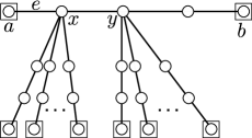
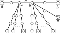
Figure 6: Two additional types of reducible configurations, T1 and T2.

Proof

Let us first consider the T1 configuration. By Claim 1 one of 1,6 is appropriate for the color of $x$, with respect to color $a$ and type of edge $e$. If $b\in\{3,4\}$, then choose $c(y)$ from $1,6$, and if $b\not\in\{3,4\}$ then choose $c(y)$ from $\{3,4\}$. By Claim 2 this works.

Let us now turn to T2. If $e$ is a near edge, we might as well contract $e$ (which implies both $x$ and $y$ will receive the same color), and reduce to Claim 6(B).

Hence we shall assume $e$ is a far edge. Assume first that coloring vertex $x$ with both $1$ and $6$ extends to the left 2-prong at $x$. If $c(x)=1$ and $c(y)=4$ does not extend to the right $2$-prongs at $y$, we may assume $b=4$. If $c(x)=6$ and $c(y)=3$ does not extend to the right $2$-prongs at $y$, we may assume $c=3$. In this case setting $c(x)=1$ and $c(y)=6$ extends to the right.

By Claim 1 we may assume that only one of $c(x)=1$ or $c(x)=6$ extends to the left 2-prong at $x$, without loss of generality the former. Now $a\neq 3$ and $a\neq 4$, and both $c(x)=3$ and $c(x)=4$ extend left. A choice of $c(x)=1,c(y)=4$ does not extend to the right $2$-prongs at $y$ only if, say, $b$ is equal to $4$. But now at least one of $c(y)=1$ or $c(y)=6$ extends to the right 2-prongs, and such a choice can be complemented with $c(x)=4$ or $c(x)=3$, respectively.

Discharging.

A minimal counterexample is the smallest possible (in terms of order) planar graph $G$ without cycles of length $\leq 9$ which is not $(8,2)$-total-threshold-colorable. A minimal counterexample $G$ does not contain reducible configurations. Further $G$ is connected and has no vertices of degree $1$. As $G$ is also not a cycle (such a cycle should be of length $\geq 9$ and should not contain a $P_{4}$), and is therefore homeomorphic to a (multi)graph of minimal degree $\geq 3$.

Let us fix its planar embedding determining its set of faces $F(G)$. Let us define initial charges: initial charge of a vertex $v$, $\gamma_{0}(v)$, is equal to $4\deg(v)-10$, and the initial charge of a face $f$, $\gamma_{0}(f)$, is equal to $\deg(f)-10$. A routine application of Euler formula shows that the total initial charge is $-20$.

As all faces have length $\geq 10$, every face is initially non-negatively charged. We shall not alter the charges of faces.

The following table shows initial charges of vertices according to their degree:

degree $\deg(v)$	2	3	4	5	6	7	$\cdots$
initial charge $\gamma_{0}(v)$	$-2$	$2$	$6$	$10$	$14$	$18$	$\cdots$

The discharging procedure will run in two phases, by $\gamma_{i}(v)$ we shall denote the charge of vertex $v$ after Phase $i$ of discharging. Informally, Phase 1 shall see that vertices of degree 2 do not have negative charges, and Phase 2 will leave only vertices of degree 3 with a possible negative charge.

Let $u,v$ be vertices of $G$. We say that $u$ and $v$ are $2$-adjacent, if $G$ contains a $u-v$-path whose (possible) internal vertices all have degree $2$. In Phase 1 we redistribute charge according to the following rule:

Rule 1: every vertex $v$ of degree $\geq 3$ sends charge $1$ to every vertex $u$ of degree $2$, for which $v$ and $u$ are $2$-adjacent.

In Phase 2 we shall apply the following rule:

Rule 2: If $u$ and $v$ are adjacent with $\gamma_{1}(u)>0,\gamma_{1}(v)<0$ then $u$ sends charge $1$ to $v$.

As every vertex $u$ of degree 2 (we also call them 2-vertices) is 2-adjacent to exactly two vertices of bigger degree, we have $\gamma_{1}(u)=0$ in this case. For a vertex $v$ of degree $\geq 3$, the discharging in Phase 1 decreases the charge of $v$ by the number of 2-vertices which are 2-adjacent to $v$.

Let $v$ be a vertex of degree $\geq 3$. A prong at $v$ is a $v-x$-path whose other end-vertex $x$ is of degree $\geq 3$ and has internal vertices of degree 2.

Claim 8

Let $v$ be a vertex of degree $\geq 3$. Then the number of 2-vertices that are 2-adjacent to $v$ is at most $2\cdot\deg(v)-3$.

Proof

By Claim 5 each prong at $v$ contains at most two vertices of degree $2$. If the shortest prong at $v$ has length $1$, then Claim 6 implies that at least one other prong has length $\leq 2$. If the shortest prong at $v$ has length $2$, then by Claim 6 we have at least four prongs that are of length $\leq 2$, and the result follows.

Now Claim 8 serves as the lower bound for vertex charges after Phase 1, and in turn prepares us for the Phase 2 of discharging.

Claim 9

1. Let $v$ be a vertex of degree $3$. If $\gamma_{1}(v)<0$, then $\gamma_{1}(v)=-1$ and the prongs at $v$ have lengths $1,2$ and $3$, respectively.

2. Let $v$ be a vertex of degree $3$. If $\gamma_{1}(v)=0$, then the prongs at $v$ have either lengths $1,1,3$ or $1,2,2$.

3. Let $v$ be a vertex of degree $3$ with its prongs of length $1,1,$ and $2$. Then $\gamma_{1}(v)=1$.

4. Let $v$ be a vertex of degree $3$ with all $3$ prongs of length $1$. Then $\gamma_{1}(v)=2$.

5. If $v$ is a vertex of degree $\geq 4$, then $\gamma_{2}(v)\geq 0$, and also $\gamma_{2}(v)$ is not smaller than the number of $1$-prongs at $v$.

Proof

Let us first prove (E). Choose a vertex $v$ with $\deg(v)\geq 4$. For every prong of length $3$, $v$ sends 2 units of charge in Phase $1$. For every shorter prong $v$ sends at most $1$ unit of charge in either Phase 1 or Phase 2. The total charge sent out of $v$ in both of the phases is by Claim 6 and Claim 8 at most $2\deg(v)-2$. Hence $\gamma_{2}(v)\geq(4\deg(v)-10)-(2\deg(v)-2)=2\deg(v)-8\geq 0$.

The other cases merely stratify vertices of degree $3$ according to the number of their $2$-neighbors of degree $2$.

Now Claim 9(E) states that every vertex $v$ of degree $\geq 4$ satisfies $\gamma_{2}(v)\geq 0$. Similarly, if a $3$-vertex $u$ is adjacent to a vertex $v$ whose degree is at least $4$, then also $\gamma_{2}(u)\geq 0$. This fact follows from either Claim 9(A) and (E) (in case $\gamma_{1}(u)<0$), or from either Claim 9(C) or (D) (if $\gamma_{1}(v)>0$) as in this case $u$ cannot send excessive charge in Phase 2.

Claim 10

No vertex $v$ has $\gamma_{2}(v)<0$ and $\gamma_{1}(v)<0$.

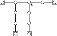
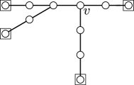
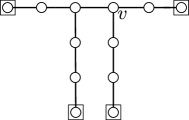
Figure 7: Negatively charged vertex $v$ after both phases induces a reducible configuration.

Proof

Let $v$ be a vertex satisfying both $\gamma_{2}(v)<0$ and $\gamma_{1}(v)<0$. By Claim 9 $\deg(v)=3$ and $v$ has prongs of length $1,2,3$. Let $u$ be the only neighbor of $v$ of degree $\neq 2$. Since $v$ has received no charge from $u$ in Phase 2 we have both $\deg(u)=3$ and $\gamma_{1}(u)\leq 0$. By Claim 9 the prongs of $u$ are of lengths $1,2,3$ or $1,1,3$ or $1,2,2$. Hence $G$ contains one of configurations shown in Fig. 7.

Now observe that these are reducible, as each matches one of T1 or T2 types of reducible configurations Claim 7.

Claim 11

No vertex $v$ has $\gamma_{2}(v)<0$ and $\gamma_{1}(v)\geq 0$.

Proof

If $\gamma_{1}(v)=0$, then also $\gamma_{2}(v)=0$, as Rule 2 does not reduce charge of a discharged vertex. By Claim 9(E) vertices of degree $\geq 4$ do not have negative charge after Phase 2.

Hence we may assume that $v$ has degree $3$, $\gamma_{1}(v)>0$, and $\gamma_{2}(v)<0$. By Claim 9(C) and (D) every neighbor $u$ of $v$ satisfies either $\deg(u)=2$ or $\deg(u)=3$ and $\gamma_{1}(u)<0$. There are exactly two possible cases and they are shown in Fig. 8.

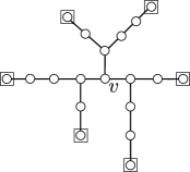
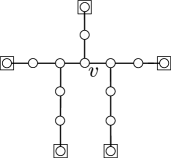
Figure 8: Negatively charged vertex $v$ after Phase 2, its charge was positive after Phase 1.

It is enough to see that there exists a color choice $c(v)$ which can be extended in the 2-prong and/or stars centered at neighbors of $v$.

Let us first settle the option shown in the right. By Claim 1 at least one of $c(v)=1$ or $c(v)=6$ extends to the top $2$-prong, and this choice also extends to the two copies of $T$, see Claim 4. The left case is even easier, as both choices $c(v)=1$ and $c(v)=6$ extend to the three copies of $T$, again by Claim 4.

Now Claim 10 and Claim 11 imply that no vertex has negative charge after Phase 2 of the discharging procedure. As the total charge remains negative and the faces cannot have negative charges we have a contradiction, which completes the proof of Theorem 4.1.

5 Unit-Cube Contact Representations of Graphs

Lemma 7

If $G$ has a unit-cube contact representation $\Gamma$ so that one face of each cube is co-planar in $\Gamma$, then any threshold subgraph of $G$ also has a unit-cube representation.

Proof

Let $H=(V,E_{H})$ be a threshold subgraph of $G=(V,E_{G})$ and let $c:V\rightarrow[1\dots r]$ be an $(r,t)$-threshold-coloring of $G$ with respect to the edge-partition $\{E_{H},E_{G}-E_{H}\}$. We now compute a unit-cube contact representation of $H$ from $\Gamma$ using $c$.

Assume (after possible rotation and translation) that the bottom face for each cube in $\Gamma$ is co-planar with the plane $z=0$; see Fig. 1(a). Also assume (after possible scaling) that each cube in $\Gamma$ has side length $t+\epsilon$, where $0<\epsilon<1$. Then we can obtain a unit-cube contact representation of $H$ from $\Gamma$ by lifting the cube for each vertex $v$ by an amount $c(v)$ so that its bottom face is at $z=c(v)$; see Fig. 1(b). Note that for any edge $(u,v)\in E_{H}$, the relative distance between the bottom faces of the cubes for $u$ and $v$ is $|c(u)-c(v)|\leq t<(t+\epsilon)$; thus the two cubes maintain contact. On the other hand, for each pair of vertices $u,v$ with $(u,v)\notin E_{H}$, one of the following two cases occurs: (i) either $(u,v)\notin E_{G}$ and their corresponding cubes remain non-adjacent as they were in $\Gamma$; or (ii) $(u,v)\in(E_{G}-E_{H})$ and the relative distance between the bottom faces of the two cubes is $|c(u)-c(v)|\geq(t+1)>(t+\epsilon)$, making them non-adjacent.

Corollary 4

Any subgraph of hexagonal and octagonal-square grid has a unit-cube contact representation.

Proof

This follows from the fact that each of these grids has a unit-cube contact representation [Fig. 9(c)–(d)] and is total-threshold-colorable [Lemmas 5, 6].

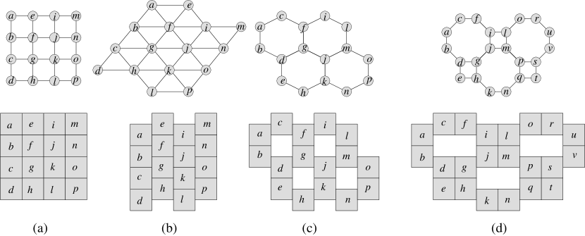
Figure 9: Unit-cube contact representations for square, triangular, hexagonal and octagonal-square grids (top-view).

Unfortunately, triangular grids are not always threshold-colorable, while for square grids, the status of the threshold-colorability is unknown. Thus we cannot use the result of Lemma 7 to find unit-cube contact representations for the subgraphs of square and triangular grids, although there are nice unit-cube contact representations for these grids with co-planar faces; see 9(a)–(b). Instead of using the threshold-coloring approach, we next show how to directly compute a unit-cube contact representation via geometric algorithms. Specifically, we describe such geometric algorithms for unit-cube contact representations for any subgraph of hexagonal and square grids.

Lemma 8

Any subgraph of a hexagonal grid has a unit-cube contact representation.

Proof

This claim follows from Corollary 4. Furthermore since hexagonal grids are subgraphs of square grids, this result can also be proven as a corollary of Lemma 9. However here we give an alternative proof by designing a geometric algorithm to construct unit-cube contact representation for subgraphs of hexagonal grids.

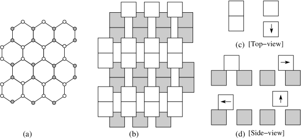
Figure 10: Construction of unit-cube representation for any subgraph of a hexagonal grid.

Let $G$ be a subgraph of a hexagonal grid $G^{*}$, as in Fig. 10(a). We first construct a unit-cube representation of $G^{*}$, where the base of each gray cube has $z$-coordinate 0 and the base of each white cube has $z$-coordinate 1; see Fig. 10(b). Call this representation $\Gamma^{*}$. We now obtain a representation of $G$ from $\Gamma^{*}$ as follows. First, we delete the cubes corresponding to the vertices of $G^{*}$ that are not in $G$. Now to delete the edges in $G^{*}$ not in $G$, we note that $G^{*}$ is bipartite. Let $A$ be a partite set of $G$. Then we can delete a set of edges by only removing the contact from cubes corresponding to vertices in $A$. Suppose $v$ is a vertex in $A$ and $R$ is the corresponding cube. Without loss of generality, assume that $R$ is a white cube. Then $R$ has (at most) three contacts: one with a white cube $w$ and two other with two gray cubes $g_{1}$, $g_{2}$. To get rid of the contact with $w$, we just shift $R$ a small distance $0<\epsilon<0.5$ away from $w$; see Fig. 10(c). On the other hand, to get rid of the contact with exactly one of $g_{1}$ and $g_{2}$, we shift $R$ away from that cube until it looses the contact, while to get rid of both the adjacencies, we shift $R$ a small distance $0<\epsilon<0.5$ upward; see Fig. 10(d).

Lemma 9

Any subgraph of a square grid has a unit-cube contact representation.

Proof

Let $G$ be a subgraph of a square grid $G^{*}$. We first construct a unit-cube representation of $G^{*}$. Note that $G^{*}$ is a bipartite graph and suppose $A$ and $B$ are its two partite sets; see Fig. 11(a). We first place cubes for the vertices of the set $A$ (white and gray vertices in the figure). Consider the $(i,j)$ coordinate system on these vertices, as illustrated in Fig. 11(a), with the center $(0,0)$ taken arbitrarily. Consider a vertex $v$ of $A$ with the coordinate $(i,j)$ in this coordinate system. We call $v$ a white vertex when $i+j$ is even; otherwise $v$ is a gray vertex. We place the cube for $v$ in the range $[x(i,j),x(i,j)+1]\times[y(i,j),y(i,j)+1]\times[z(i,j),z(i,j)+1]$; where $x(i,j)=[\delta i+(2-\delta)j]$, $y(i,j)=[(2-\delta)i-\delta j]$, $0<\delta<0.5$ and $z(i,j)=0.5$ if $v$ is a white vertex, otherwise $z(i,j)=0$. Each black vertex has two adjacent white and two adjacent gray vertices and we place its unit cube between the cubes for four adjacent vertices with $z$-coordinate 0.25; see Fig. 11(b).

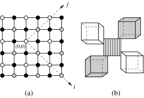
Figure 11: Construction of unit-cube representation for any subgraph of a square grid.

We now modify this representation of $G^{*}$ to compute a representation for $G$. First we delete the cubes for the vertices of $G^{*}$ not in $G$. Then to remove contacts corresponding to the edges of $G^{*}$ not in $G$, we move cubes for the black vertices. Suppose $v_{b}$ is such a black vertex and its two adjacent white vertices are at coordinates $(i,j)$, $(i+1,j+1)$; while its two adjacent gray vertices are at coordinates $(i,j+1)$, $(i+1,j)$. Call the cube for the black vertex $R_{b}$ and let $R(x,y)$ denote the cubes for the white or gray vertex at coordinate $(x,y)$. If $v_{b}$ has degree $4$ in $G$, we don’t have to move $R_{b}$. Again if $v_{b}$ has degree 0 in $G$, we move $R_{b}$ outside the boundary of $\Gamma$. Otherwise depending on the incident edges of $v_{b}$ present in $G$, we need to get rid of some of the contacts with $R_{b}$. We show how to do this in cases.

Case 1: $v_{b}$ has degree 3 in $G$. Assume that the incident edge of $v_{b}$ in $G^{*}$ missing in $G$ is with $v(i,j)$. Then we shift $R_{b}$ downward until its topmost plane has $z$-coordinate 0.5 and then we shift $R_{b}$ in the $xy$-plane by a small amount $\epsilon$ away from $R(i,j)$, where $0<\epsilon<\delta$.

Case 2: $v_{b}$ has degree 2 in $G$. If the two incident edges of $v_{b}$ missing in $G$ are both with white (gray) vertices, then we shift $R_{b}$ downwards (upwards) until it looses contacts with both its white (gray) neighbors. Otherwise, assume that the two incident edges of $v_{b}$ missing in $G$ are with $v(i,j)$ and $v(i,j+1)$. In this case, we shift $R_{b}$ downward until its topmost plane has $z$-coordinate 0.5 and then we shift $R_{b}$ in the $xy$-plane away from both $R(i,j)$ and $R(i,j+1)$ until it looses contact with both of them.

Case 3: $v_{b}$ has degree 1 in $G$. Suppose the incident edges of $v_{b}$ missing from $G$ are with $v(i,j)$, $v(i,j+1)$ and $v(i+1,j)$. We then first shift $R_{b}$ upward until its bottommost plane has $z$-coordinate is in the open interval $(1,1.5)$ so that it looses contacts with both $R(i,j+1)$ and $R(i+1,j)$. Finally we move $R_{b}$ away from $R(i,j)$ until it looses the contact with $R(i,j)$.

To summarize the results in this section:

Theorem 5.1

Any subgraph of the square, hexagonal and octagonal-square grid has a unit-cube contact representation.

6 Conclusion and Open Problems

We introduced a new graph coloring problem, called threshold-coloring, that generates spanning subgraphs from an input graph where the edges of the subgraph are implied by small absolute value difference between the colors of the endpoints. We showed that any spanning subgraph of trees, some planar grids, and planar graphs without cycles of length $\leq 9$ can be generated in this way; for other classes like triangular and square-triangle grids, we showed that this is not possible. We also considered different variants of the problem and noted relations with other well-known graph coloring and graph-theoretic problems. Finally we use the threshold-coloring problem to find unit-cube contact representation for all the subgraphs of some planar grids. The following is a list of some interesting open problems and future work.

1. Some classes of graphs are total-threshold-colorable, while others are not. There are many classes for which the problem remains open; see Table 1 for some examples. A particularly interesting class is the square grid: does any subgraph of a square grid have a threshold-coloring?

2. Theorem 4.1 implies that any planar graph without cycles of length $\leq 9$ is total-threshold-colorable. On the other hand, all our examples of non-threshold-colorable in Fig. 3 contain triangles. Can we reduce this gap by identifying the minimum cycle-length (girth) in a planar graph that guarantees total-threshold-colorability?

3. Can we efficiently recognize graphs that are threshold-colorable?

4. Is there a good characterization of threshold-colorable graphs?

5. The triangular and square-triangular grid are not total-threshold-colorable and we cannot use threshold-colorability to find unit-cube contact representations; can we give a geometric algorithm (such as those in Section 5 for square and hexagonal grids) to directly compute such representations?

Acknowledgments: We thank Torsten Ueckerdt, Carola Winzen and Michael Bekos for discussions about different variants of the threshold-coloring problem.

References

- [1] A. Brandstädt, V. B. Le, and J. P. Spinrad. Graph classes: a survey. Society for Industrial and Applied Mathematics, 1999.
- [2] D. Bremner, W. Evans, F. Frati, L. Heyer, S. Kobourov, W. Lenhart, G. Liotta, D. Rappaport, and S. Whitesides. On representing graphs by touching cuboids. In Graph Drawing, pages 187–198, 2012.
- [3] C. M. H. de Fegueiredo, J. Meidanis, and C. P. de Mello. A linear-time algorithm for proper interval graph recognition. Information Processing Letter, 56(3):179–184, 1995.
- [4] S. Felsner and M. C. Francis. Contact representations of planar graphs with cubes. In Symposium on Computational geometry, pages 315–320, 2011.
- [5] J. Fiala, T. Kloks, and J. Kratochvíl. Fixed-parameter complexity of -labelings. Discrete Applied Mathematics, 113(1):59–72, 2001.
- [6] J. Fiala, J. Kratochvíl, and A. Proskurowski. Systems of distant representatives. Discrete Applied Mathematics, 145(2):306 – 316, 2005.
- [7] M. C. Golumbic, H. Kaplan, and R. Shamir. On the complexity of DNA physical mapping. Advances in Applied Mathematics, 15(3):251–261, 1994.
- [8] M. C. Golumbic, H. Kaplan, and R. Shamir. Graph sandwich problems. Journal of Algorithms, 19(3):449–473, 1995.
- [9] J. R. Griggs and R. K. Yeh. Labelling graphs with a condition at distance 2. SIAM Journal on Discrete Mathematics, 5(4):586–595, 1992.
- [10] W. Hale. Frequency assignment: Theory and applications. Proceedings of the IEEE, 68(12):1497–1514, 1980.
- [11] P. L. Hammer, U. N. Peled, and X. Sun. Difference graphs. Discrete Applied Mathematics, 28(1):35–44, 1990.
- [12] P. Hell, R. Shamir, and R. Sharan. A fully dynamic algorithm for recognizing and representing proper interval graphs. In European Symposium on Algorithms, pages 527–539, 1999.
- [13] V. B. Le and D. Rautenbach. Integral mixed unit interval graphs. In Computing and Combinatorics, pages 495–506, 2012.
- [14] N. V. R. Mahadev and U. N. Peled. Threshold Graphs and Related Topics. North Holland, 1995.
- [15] F. Roberts. From garbage to rainbows: Generalizations of graph coloring and their applications. Graph Theory, Combinatorics, and Applications, 2:1031–1052, 1991.
- [16] C. Thomassen. Interval representations of planar graphs. Journal of Combinatorial Theory, Series B, 40(1):9 – 20, 1986.