Anisotropic universes in the ghost-free bigravity

Abstract

We study Bianchi cosmologies in the ghost-free bigravity theory assuming both metrics to be homogeneous and anisotropic, of the Bianchi class A, which includes types I,II,VI₀,VII₀,VIII, and IX. We assume the universe to contain a radiation and a non-relativistic matter, with the cosmological term mimicked by the graviton mass. We find that, for generic initial values leading to a late-time self-acceleration, the universe approaches a state with non-vanishing anisotropies. The anisotropy contribution to the total energy density decreases much slower than in General Relativity and shows the same falloff rate as the energy of a non-relativistic matter. The solutions show a singularity in the past, and in the Bianchi IX case the singularity is approached via a sequence of Kasner-like steps, which is characteristic for a chaotic behavior.

I Introduction

The recent discovery of the ghost-free massive gravity theory de Rham et al. (2011) and its bigravity generalization Hassan and Rosen (2012a) has revived the old idea that gravitons can have a small mass Fierz and Pauli (1939). Theories with massive gravitons were for a long time considered as pathological, mainly because they exhibit the Boulware-Deser (BD) ghost – an unphysical negative norm state in the spectrum Boulware and Deser (1972). However, it turns out that the presence of the BD ghost is not mandatory, and the theories of de Rham et al. (2011); Hassan and Rosen (2012a) are free of this pathology. A careful analysis shows that the number of propagating degrees of freedom in these theories agrees with the number of graviton polarizations Hassan and Rosen (2012b); *Golovnev:2011aa; *Kluson:2012wf; *Hassan:2012qv; *Hassan:2011ea. This does not mean that all solutions are stable, since there could be other instabilities, which should be checked in each particular case. However, since the most dangerous BD ghost instability is absent, the ghost-free theories of bigravity and massive gravity can be considered as healthy physical models for interpreting the observational data.

Theories with massive gravitons can be used in order to explain the observed acceleration of our universe Riess et al. (1998); *0004-637X-517-2-565. This effect can be accounted for by introducing a cosmological term to the Einstein equations, however, this poses the problem of explaining the origin and value of this term. An alternative possibility is to consider modifications of General Relativity, and theories with massive gravitons are natural candidates for this, since the graviton mass can effectively manifest itself as a small cosmological term Damour et al. (2002). This justifies interest towards studying cosmological solutions with massive gravitons.

The known cosmologies with massive gravitons can be divided into two types. The first type is provided by solutions described by two metrics which are not simultaneously diagonal. For these solutions the graviton mass gives rise just to a constant term in the Einstein equations and to nothing else, at least for the homogeneous and isotropic backgrounds. Such solutions had been first obtained without matter Koyama et al. (2011a); *Koyama:2011yg, while later the special Chamseddine and Volkov (2011),D’Amico et al. (2011),Kobayashi et al. (2012); *Gratia:2012wt and also general Volkov (2012a); *Volkov:2012zb solutions including a matter source were found. For these solutions the mater dominates at early times, when the universe is small, while later the mass density decreases and the effective cosmological term becomes dominant, leading to a self-acceleration. Such solutions exist for all (open, closed and flat) Friedmann-Lemâtre-Robertson-Walker (FLRW) types, both in massive gravity and bigravity. However, perturbations around these backgrounds are expected to be inhomogeneous – due to the non-diagonal metric components, hence solutions of this type are sometimes called ‘inhomogeneous’ D’Amico et al. (2011).

For the second type solutions both metrics are diagonal and of the FLRW type. In this case the effect of the graviton mass can be more complex and reduces to that of a cosmological term only at late times. Such solutions have a somewhat narrow existence range. For example, in massive gravity they exist only for the spatially open FLRW type Gumrukcuoglu et al. (2011); *DeFelice:2012mx, and although in bigravity they exist for all spatial types Volkov (2012c),von Strauss et al. (2012); *Comelli:2011zm; *Comelli:2012db; *Khosravi:2012rk, they do not admit the limit where one of the two metrics becomes flat. The bigravity solutions exhibit rather complex features and show several branches. There are physical solutions for which the matter dominates at early times, while the graviton mass becomes essential later. In addition, there are also exotic solutions for which the graviton mass contribution is dominant at all times.

Up to now, cosmologies with massive gravitons have been studied mainly in the FLRW limit. It may be important to extend the analysis to more general spacetimes. For example, one may wonder whether the FLRW universe is stable against anisotropic or inhomogeneous perturbations Gumrukcuoglu et al. (2012),Sakakihara et al. (2012). Another motivation is the so-called cosmic no-hair conjecture. In General Relativity (GR) with a cosmological term the de Sitter spacetime is expected to be an attractor Starobinsky (1983); *Muller:1989rp; *Wald:1983ky; *Kitada:1991ih; *Kitada:1992uh. In massive gravity or bigravity the graviton mass gives rise to a cosmological term at late times, and so the acceleration of the universe can be explained by the de Sitter expansion. However, since the graviton mass is not exactly a cosmological term, one may wonder whether the de Sitter space is still an attractor for generic initial values. An interesting byproduct in such studies can be an observational relic – if small anisotropy remains in the accelerating phase, it could be observed Gumrukcuoglu et al. (2012).

In what follows, we undertake a systematic analysis of anisotropic cosmologies in the ghost-free bigravity Hassan and Rosen (2012a), assuming both metrics to be simultaneously diagonal and of the same Bianchi type within the Bianchi class A, which includes types I,II,VI₀,VII₀,VIII, and IX.

As a starting point, we find exact solutions for the Bianchi I type for which the two metrics have identically the same anisotropies, which however requires to fine-tune the two matter sources. Then we attack the problem numerically and discover that, even in the presence of a matter and for all other Bianchi types of class A, the equal anisotropy configurations play the role of late time attractors. Specifically, starting form arbitrary initial data, the anisotropies approach equal and constant values. For Bianchi I solutions constant anisotropies can be scaled away, but not for other Bianchi types, so that generic homogeneous spacetimes run into anisotropic states.

We find that the shears approach zero exponentially fast as the universe approaches the de Sitter phase. However, since the anisotropies do not approach zero but oscillate around constant values, the shear contribution to the total energy density decreases only as an inverse cube of the size of the universe. This is the same falloff rate as for a non-relativistic matter, whereas in GR shears decrease as the inverse sixth power of the size of the universe. Therefore, the anisotropy effect could be observable, and so it would be interesting to compare our predictions with observations. Since the anisotropy contribution shows the same falloff rate as a cold dark matter, it is tempting to think that the latter could in fact be the effect of the anisotropies, although it is unclear if this interpretation can also explain the dark matter clustering.

The rest of the paper is organized as follows. In the next two sections we describe the ghost-free bigravity Hassan and Rosen (2012a), the Bianchi cosmologies, and derive the field equations in the case where the two metrics are simultaneously diagonal and of the same Bianchi type of class A. In Section IV we study exact solutions of these equations for the Bianchi I type. First, these are solutions with proportional metrics, they are the same as in GR. Next, these are solutions with identical anisotropies for the two metrics, which can be of the FLRW type Volkov (2012c),von Strauss et al. (2012); *Comelli:2011zm; *Comelli:2012db; *Khosravi:2012rk if anisotropies vanish. In Section V we present the generalization to the other Bianchi types of class A. We describe our procedure for the numerical integration – the dynamical system formulation of the problem and the implementation of the initial values constraints, after which we present our numerical results. Section VI contains concluding remarks, while in the Appendix we describe the Bianchi I solutions in GR and also give the details of the dynamical system formulation.

We set $\hbar=c=1$ and use the sign conventions of Misner-Thorne-Wheeler. The space and time scale is chosen to be the inverse graviton mass.

II The ghost-free bigravity

The theory is defined on a four-dimensional spacetime manifold equipped with two metrics, ${\bf g_{\mu\nu}}$ and ${\bf f_{\mu\nu}}$. The kinetic term of each metric is chosen to be of the standard Einstein-Hilbert form, while the interaction between them is parametrized by a scalar function of the tensor

$$\gamma^{\mu}_{~{}\nu}=\sqrt{{\bf g}^{\mu\alpha}{\bf f}_{\alpha\nu}},$$ (2.1)

where ${\bf g}^{\mu\nu}$ is the inverse of ${\bf g}_{\mu\nu}$ and the square root is understood in the sense that

$$(\gamma^{2})^{\mu}_{~{}\nu}\equiv\gamma^{\mu}_{~{}\alpha}\gamma^{\alpha}_{~{}\nu}={\bf g}^{\mu\alpha}{\bf f}_{\alpha\nu}.$$ (2.2)

The action is

$$S[{\bf g},{\bf f},{\rm matter}]$$

$$~{}~{}=\frac{1}{2\kappa_{g}^{2}}\,\int d^{4}x\,\sqrt{-{\bf g}}\,R({\bf g})+\frac{1}{2\kappa_{f}^{2}}\,\int d^{4}x\,\sqrt{-{\bf f}}\,{\cal R}({\bf f})$$

$$~{}~{}-\frac{m^{2}}{\kappa^{2}}\int d^{4}x\,\sqrt{-{\bf g}}\,\mathscr{U}[{\bf g},{\bf f}]\,$$ (2.3)

$$~{}~{}+S^{[\rm m]}_{g}[{\bf g},{\rm g\mathchar 45\relax matter}]+S^{[\rm m]}_{f}[{\bf f},{\rm f\mathchar 45\relax matter}]\,,$$

where $R$ and ${\cal R}$ are the Ricci scalars for ${\bf g}_{\mu\nu}$ and ${\bf f}_{\mu\nu}$, respectively, $\kappa_{g}^{2}=8\pi G$ and $\kappa_{f}^{2}=8\pi{\cal G}$ are the corresponding gravitational couplings, while $\kappa^{2}=\kappa_{g}^{2}+\kappa_{f}^{2}$ and $m$ is the graviton mass. The interaction between the two metrics is given by

$$\mathscr{U}=\sum_{k=0}^{4}b_{k}\,\mathscr{U}_{k}(\gamma),$$ (2.4)

where $b_{k}$ are parameters, while $\mathscr{U}_{k}(\gamma)$ are defined by the following relations

$$\mathscr{U}_{0}(\gamma) = -\frac{1}{4!}\,\epsilon_{\mu\nu\rho\sigma}\epsilon^{\mu\nu\rho\sigma}=1,$$ (2.5)

$$\mathscr{U}_{1}(\gamma) = -\frac{1}{3!}\,\epsilon_{\mu\nu\rho\sigma}\epsilon^{\alpha\nu\rho\sigma}\gamma^{\mu}_{~{}\alpha}=\sum_{A}\lambda_{A}=[\gamma],$$

$$\mathscr{U}_{2}(\gamma) = -\frac{1}{2!}\,\epsilon_{\mu\nu\rho\sigma}\epsilon^{\alpha\beta\rho\sigma}\gamma^{\mu}_{~{}\alpha}\gamma^{\nu}_{~{}\beta}=\sum_{A<B}\lambda_{A}\lambda_{B}$$

$$= \frac{1}{2!}([\gamma]^{2}-[\gamma^{2}]),$$

$$\mathscr{U}_{3}(\gamma) = -\frac{1}{3!}\,\epsilon_{\mu\nu\rho\sigma}\epsilon^{\alpha\beta\gamma\sigma}\gamma^{\mu}_{~{}\alpha}\gamma^{\nu}_{~{}\beta}\gamma^{\rho}_{~{}\gamma}=\sum_{A<B<C}\lambda_{A}\lambda_{B}\lambda_{C}$$

$$= \frac{1}{3!}([\gamma]^{3}-3[\gamma][\gamma^{2}]+2[\gamma^{3}]),$$

$$\mathscr{U}_{4}(\gamma) = -\frac{1}{4!}\,\epsilon_{\mu\nu\rho\sigma}\epsilon^{\alpha\beta\gamma\delta}\gamma^{\mu}_{~{}\alpha}\gamma^{\nu}_{~{}\beta}\gamma^{\rho}_{~{}\gamma}\gamma^{\sigma}_{~{}\delta}=\lambda_{0}\lambda_{1}\lambda_{2}\lambda_{3}$$

$$= \frac{1}{4!}([\gamma]^{4}-6[\gamma]^{2}[\gamma^{2}]+8[\gamma][\gamma^{3}]+3[\gamma^{2}]^{2}-6[\gamma^{4}])\,.$$

Here $\lambda_{A}$ ($A=0,1,2,3$) are eigenvalues of $\gamma^{\mu}_{~{}\nu}$, and, using the hat to denote matrices, we have defined

$$[\gamma]={\rm tr}(\hat{\gamma})=\gamma^{\mu}_{~{}\mu},~{}~{}~{}~{}[\gamma^{k}]={\rm tr}(\hat{\gamma}^{k})=(\gamma^{k})^{\mu}_{~{}\mu}\,.$$ (2.6)

The above choice of the interaction potential $\mathscr{U}$ insures that the BS ghost is absent Hassan and Rosen (2012b); *Golovnev:2011aa; *Kluson:2012wf; *Hassan:2012qv; *Hassan:2011ea. We have also assumed a g-matter and an f-matter interacting, respectively, only with ${\bf g}_{\mu\nu}$ and with ${\bf f}_{\mu\nu}$. One cannot have a matter coupled to both metrics at the same time, since the BD ghost would come back in this case, whereas our choice is ghost-free Hassan and Rosen (2012a). In addition, this choice preserves the equivalence principle, since the g-matter follows geodesics of the g-metric and the f-matter follows f-geodesics. Although it is sometimes convenient to have only a g-matter and choose the f-sector to be empty, nothing forbids to have both matter types at the same time.

It is also useful to express the interaction in terms of ${\cal K}^{\mu}_{\nu}=\delta^{\mu}_{\nu}-\gamma^{\mu}_{~{}\nu}$,

$$\mathscr{U}=\sum_{k=0}^{4}c_{k}\,\mathscr{U}_{k}({\cal K}),$$ (2.7)

where $\mathscr{U}_{k}({\cal K})$ are defined by the same expressions as in (2.5), up to the replacement $\lambda_{A}\to\mu_{A}=1-\lambda_{A}$ and $\gamma\to{\cal K}$, where $\mu_{A}$’s are eigenvalues of ${\cal K}^{\mu}_{~{}\nu}$. The parameters $c_{k}$ are related to $b_{k}$ as

$$c_{0} = b_{0}+4b_{1}+6b_{2}+4b_{3}+b_{4},$$

$$c_{1} = -(b_{1}+3b_{2}+3b_{3}+b_{4}),$$

$$c_{2} = b_{2}+2b_{3}+b_{4},$$

$$c_{3} = -(b_{3}+b_{4}),$$

$$c_{4} = b_{4}\,,$$ (2.8)

with the inverse expressions

$$b_{0} = c_{0}+4c_{1}+6c_{2}+4c_{3}+c_{4},$$

$$b_{1} = -(c_{1}+3c_{2}+3c_{3}+c_{4}),$$

$$b_{2} = c_{2}+2c_{3}+c_{4},$$

$$b_{3} = -(c_{3}+c_{4}),$$

$$b_{4} = c_{4}.$$ (2.9)

In the weak field limit, when ${\bf g}_{\mu\nu}\approx{\bf f}_{\mu\nu}\approx\eta_{\mu\nu}$, the tensor ${\cal K}$ tends to zero while $\mathscr{U}_{k}\sim{\cal K}^{k}$ so that Eq.(2.7) gives the interaction in terms of powers of deviation from the flat space. We require the flat space to be a solution of the field equations, which is only possible if

$$c_{0}=c_{1}=0,$$ (2.10)

while the quadratic part of the interaction should reproduce the Fierz-Pauli term,

$$+\frac{m^{2}}{2}([{\cal K}]^{2}-[{\cal K}^{2}]),$$ (2.11)

which fixes the normalization

$$c_{2}=-1.$$ (2.12)

The above choice implies that the bare cosmological constant is zero, so that a non-zero cosmological term can only be of a dynamical origin, due to the graviton mass contribution. Terms proportional to $c_{3}$ and$c_{4}$ can be kept, so that

$$b_{0}=4c_{3}+c_{4}-6,~{}~{}b_{1}=3-3c_{3}-c_{4},~{}~{}$$

$$b_{2}=2c_{3}+c_{4}-1,~{}~{}b_{3}=-(c_{3}+c_{4}),~{}~{}$$

$$b_{4}=c_{4}.$$ (2.13)

II.1 Field equations

Assuming the spacetime coordinates $x^{\mu}$ to be dimensionless, the metrics ${\bf g}_{\mu\nu}$, ${\bf f}_{\mu\nu}$ have the dimension of length squared. To pass to dimensionless quantities, we make a conformal rescaling

$${\bf g}_{\mu\nu}=\frac{1}{m^{2}}\,g_{\mu\nu},~{}~{}~{}~{}~{}{\bf f}_{\mu\nu}=\frac{1}{m^{2}}\,f_{\mu\nu}.$$ (2.14)

Varying the action then gives the field equations

$$G_{\mu\nu} = \kappa_{g}^{2}\left[T_{\mu\nu}^{[\gamma]}+\frac{1}{m^{2}}\,\underline{T}^{\rm[m]}_{~{}\mu\nu}\right]\,,$$ (2.15)

$${\cal G}_{\mu\nu} = \kappa_{f}^{2}\left[{\cal T}_{\mu\nu}^{[\gamma]}+\frac{1}{m^{2}}\,\underline{\cal T}^{\rm[m]}_{~{}\mu\nu}\right]\,,$$ (2.16)

where $G_{\mu\nu}$ and ${\cal G}_{\mu\nu}$ are the Einstein tensors for $g_{\mu\nu}$ and $f_{\mu\nu}$. The graviton energy-momentum tensors are

$$T_{\mu\nu}^{[\gamma]}=\frac{1}{\kappa^{2}}\left(2\,\frac{\delta\mathscr{U}}{\delta g^{\mu\nu}}-\mathscr{U}\,g_{\mu\nu}\right),$$

$${\cal T}_{\mu\nu}^{[\gamma]}=2\,\frac{1}{\kappa^{2}}\frac{\sqrt{-g}}{\sqrt{-f}}\,\frac{\delta\mathscr{U}}{\delta f^{\mu\nu}}\,.$$ (2.17)

In order to perform the variations here, one uses the relations

$$\frac{\delta[\gamma^{n}]}{\delta g^{\mu\nu}}=\frac{n}{2}\,g_{\mu\alpha}(\gamma^{n})^{\alpha}_{~{}\nu}=\frac{n}{2}\,g_{\nu\alpha}(\gamma^{n})^{\alpha}_{~{}\mu},$$

$$\frac{\delta[\gamma^{n}]}{\delta f^{\mu\nu}}=-\frac{n}{2}\,f_{\mu\alpha}(\gamma^{n})^{\alpha}_{~{}\nu}=-\frac{n}{2}\,f_{\nu\alpha}(\gamma^{n})^{\alpha}_{~{}\mu}\,,$$ (2.18)

which can be obtained by varying the definition $\gamma^{\mu}_{~{}\nu}=\sqrt{{g}^{\mu\alpha}{f}_{\alpha\nu}}$ and using the properties of the trace. Introducing the angle $\eta$ such that

$$\kappa_{g}=\kappa\cos\eta,~{}~{}~{}~{}~{}~{}\kappa_{f}=\kappa\sin\eta,$$ (2.19)

one obtains dimensionless quantities

$$\kappa_{g}^{2}T^{[\gamma]\mu}_{~{}~{}~{}~{}~{}\nu}=\cos^{2}\eta(\,\tau^{\mu}_{~{}\nu}-\mathscr{U}\,\delta^{\mu}_{\nu}),$$

$$\kappa_{f}^{2}{\cal T}^{[\gamma]\mu}_{~{}~{}~{}~{}~{}\nu}=-\sin^{2}\eta\,\frac{\sqrt{-g}}{\sqrt{-f}}\,\tau^{\mu}_{~{}\nu}\,,$$ (2.20)

where $T^{\mu}_{~{}\nu}=g^{\mu\alpha}T_{\alpha\nu}$ and ${\cal T}^{\mu}_{~{}\nu}=f^{\mu\alpha}{\cal T}_{\alpha\nu}$ while

$$\tau^{\mu}_{~{}\nu} = \{b_{1}\,\mathscr{U}_{0}+b_{2}\,\mathscr{U}_{1}+b_{3}\,\mathscr{U}_{2}+b_{4}\,\mathscr{U}_{3}\}\gamma^{\mu}_{~{}\nu}$$

$$- \{b_{2}\,\mathscr{U}_{0}+b_{3}\,\mathscr{U}_{1}+b_{4}\,\mathscr{U}_{2}\}(\gamma^{2})^{\mu}_{~{}\nu}$$

$$+ \{b_{3}\,\mathscr{U}_{0}+b_{4}\,\mathscr{U}_{1}\}(\gamma^{3})^{\mu}_{~{}\nu}$$

$$- b_{4}\,\mathscr{U}_{0}\,(\gamma^{4})^{\mu}_{~{}\nu}$$ (2.22)

with $\mathscr{U}_{k}\equiv\mathscr{U}_{k}(\gamma)$. The matter energy-momentum tensors $\underline{T}^{\rm[m]}_{~{}\mu\nu}$ and $\underline{\cal T}^{\rm[m]}_{~{}\mu\nu}$ are dimensionful, we assume them to be of perfect fluid type. However, they enter the equations only via dimensionless combinations

$$\frac{\kappa_{g}^{2}}{m^{2}}\,\underline{T}^{\rm[m]\mu}_{~{}~{}~{}~{}~{}\nu}\equiv T^{\rm[m]\mu}_{~{}~{}~{}~{}~{}\nu}=(\rho_{g}+P_{g}){U}^{\mu}{U}_{\nu}+P_{g}\,\delta^{\mu}_{\nu}$$

$$\frac{\kappa_{f}^{2}}{m^{2}}\,\underline{\cal T}^{\rm[m]\mu}_{~{}~{}~{}~{}~{}\nu}\equiv{\cal T}^{\rm[m]\mu}_{~{}~{}~{}~{}~{}\nu}=(\rho_{f}+P_{f}){\cal U}^{\mu}{\cal U}_{\nu}+P_{f}\,\delta^{\mu}_{\nu}\,.~{}~{}~{}~{}~{}~{}~{}~{}$$ (2.23)

As a result, from now on we shall be considering the field equations (2.15),(2.16) expressed entirely in terms of dimensionless quantities.

The diffeomorphism invariance of the matter terms in the action implies the conservation conditions

$$\stackrel{{\scriptstyle(g)}}{{\nabla}}_{\mu}T^{\rm[m]\mu}_{~{}~{}~{}~{}~{}\nu}=0,~{}~{}~{}~{}~{}\stackrel{{\scriptstyle(f)}}{{\nabla}}_{\mu}{\cal T}^{\rm[m]\mu}_{~{}~{}~{}~{}~{}\nu}=0\,,$$ (2.24)

where $\stackrel{{\scriptstyle(g)}}{{\nabla}}$ and $\stackrel{{\scriptstyle(f)}}{{\nabla}}$ are covariant derivatives with respect to $g_{\mu\nu}$ and $f_{\mu\nu}$. The Bianchi identities for (2.15) then imply that

$$\stackrel{{\scriptstyle(g)}}{{\nabla}}_{\mu}\!T^{[\gamma]\mu}_{~{}~{}~{}~{}~{}\nu}=0.$$ (2.25)

Similarly, the Bianchi identities for equations (2.16) imply that $\stackrel{{\scriptstyle(f)}}{{\nabla}}_{\mu}\!{\cal T}^{[\gamma]\mu}_{~{}~{}~{}~{}~{}\nu}=0$, but in fact this condition is not independent and follows from (2.25) in view of the diffeomorphism invariance of the interaction term in the action.

III Bianchi Spacetimes

In what follows, we shall assume both metrics to be homogeneous but anisotropic, that is, invariant under a three-parameter translation group G₃ acting on the 3-space. The group is generated by three vector fields $e_{a}$ satisfying commutation relations

$$[e_{a},e_{b}]=C^{c}_{~{}ab}e_{c}$$ (3.1)

with constant structure coefficients $C^{c}_{~{}ab}$. Such groups have been all classified by Bianchi. The Jacobi identities imply that structure coefficients can be parameterized as

$$C^{c}_{~{}ab}=n^{cd}\epsilon_{dab}+a(\delta^{1}_{a}\delta_{b}^{c}-\delta^{1}_{b}\delta_{a}^{c})\,$$ (3.2)

with $n^{ab}={\rm diag}[n^{(1)},n^{(2)},n^{(3)}]$. The different choices of the four parameters $n^{(1)}$, $n^{(2)}$, $n^{(3)}$, $a$ correspond to the nine Bianchi types.

Denoting $\omega^{a}$ the 1-forms dual to $e_{a}$, the two metrics can be parameterized as

$$ds_{g}^{2} = -\alpha(t)^{2}dt^{2}+h_{ab}(t)\,\omega^{a}\otimes\omega^{b},$$

$$ds_{f}^{2} = -{\mathcal{A}}(t)^{2}dt^{2}+{\cal H}_{ab}(t)\,\omega^{a}\otimes\omega^{b}\,.$$ (3.3)

In this paper, we discuss only the class A Bianchi models, for which the parameter $a$ in (3.2) vanishes. These include types I, II, VI₀, VII₀, VIII, IX. For these types tensors $h_{ab}$ and ${\cal H}_{ab}$ can be chosen to be diagonal, and this guarantees that $G_{0a}=0$ and ${\cal G}_{0a}=0$, so that there are no energy fluxes. To achieve a similar no-flux condition for the type B (tilted) Bianchi classes with $a\neq 0$, one has to either let $h_{ab}$ and ${\cal H}_{ab}$ be non-diagonal, or to impose constraints on the otherwise independent values of their components.

Let $h_{ab}$, ${\cal H}_{ab}$ be diagonal matrices,

$$h_{ab} = {\rm diag}[\alpha_{1}^{\,2},\alpha_{2}^{\,2},\alpha_{3}^{\,2}],$$

$${\cal H}_{ab} = {\rm diag}[{\cal A}_{1}^{\,2},{\cal A}_{2}^{\,2},{\cal A}_{3}^{\,2}],$$

and introduce

$$Q^{a}_{~{}b} = 2\,{\rm diag}\left[\frac{\dot{\alpha_{1}}}{\alpha_{1}},\frac{\dot{\alpha_{2}}}{\alpha_{3}},\frac{\dot{\alpha_{3}}}{\alpha_{3}}\right]\,,$$

$${\cal Q}^{a}_{~{}b} = 2\,{\rm diag}\left[\frac{\dot{{\cal A}_{1}}}{{\cal A}_{1}},\frac{\dot{{\cal A}_{2}}}{{\cal A}_{3}},\frac{\dot{{\cal A}_{3}}}{{\cal A}_{3}}\right]\,,~{}~{}$$

where the dot denotes the time derivative. The non-zero projections $R^{A}_{~{}B}$ and ${\cal R}^{A}_{~{}B}$ of the Ricci tensors on the tetrad base $\Theta^{A}=(dt,\omega^{a})$ and $E_{A}=(\partial_{t},e_{a})$ read

$$R^{0}_{~{}0}=\frac{[\dot{Q}]}{2}+\frac{[Q^{2}]}{4},~{}~{}R^{a}_{~{}b}=\,\frac{\left(\sqrt{h}Q^{a}_{~{}b}\right)^{\centerdot}}{2\alpha\sqrt{h}}+\overset{(3)~{}}{R^{a}_{~{}b}},~{}$$

$${\cal R}^{0}_{~{}0}=\frac{[\dot{\cal Q}]}{2}+\frac{[{\cal Q}^{2}]}{4},~{}~{}{\cal R}^{a}_{~{}b}=\frac{\left(\sqrt{\cal H}{\cal Q}^{a}_{~{}b}\right)^{\centerdot}}{2\sqrt{\cal H}{\cal A}}+\overset{(3)~{}}{{\cal R}^{a}_{~{}b}}.~{}~{}~{}$$ (3.4)

Here the bracketed quantities are calculated according to (2.6), while the three-dimensional Ricci tensors

$$h\,\overset{(3)~{}}{R^{a}_{~{}b}}=2(N^{2})^{a}_{~{}b}-[N]\,N^{a}_{~{}b}-([N^{2}]-{1\over 2}[N]^{2})\delta^{a}_{~{}b}\,,~{}~{}~{}~{}$$

$${\cal H}\,\overset{(3)~{}}{{\cal R}^{a}_{~{}b}}=2({\cal N}^{2})^{a}_{~{}b}-[{\cal N}]\,{\cal N}^{a}_{~{}b}-([{\cal N}^{2}]-{1\over 2}[{\cal N}]^{2})\delta^{a}_{~{}b}\,,~{}~{}~{}~{}$$ (3.5)

where

$$N^{a}_{~{}b}=n^{ac}h_{cb},~{}~{}~{}~{}{\cal N}^{a}_{~{}b}=n^{ac}{\cal H}_{cb}.$$ (3.6)

The Ricci scalars are

$$\overset{\tiny(3)}{R}=\frac{1}{2h}\left([N]^{2}-2[N^{2}]\right),~{}~{}\overset{\tiny(3)}{\cal R}=\frac{1}{2{\cal H}}\left([{\cal N}]^{2}-2[{\cal N}^{2}]\right).~{}~{}$$ (3.7)

The non-trivial tetrad projections $\gamma^{A}_{~{}B}$ of the tensor $\gamma^{\mu}_{~{}\nu}=\sqrt{g^{\mu\alpha}f_{\alpha\nu}}$ are

$$\gamma^{A}_{~{}B}={\rm diag}\left[\frac{{\cal A}}{\alpha},\frac{{\cal A}_{1}}{\alpha_{1}},\frac{{\cal A}_{2}}{\alpha_{2}},\frac{{\cal A}_{3}}{\alpha_{3}}\right].$$ (3.8)

Using this in Eqs.(2.4),(2.5),(II.1),(II.1) reveals that non-trivial tetrad components of the energy-momentum tensors $T^{[\gamma]\mu}_{~{}~{}~{}~{}~{}\nu}$ and ${\cal T}^{[\gamma]\mu}_{~{}~{}~{}~{}~{}\nu}$ are also diagonal. For example, the non-trivial tetrad projections of $\tau^{\mu}_{~{}\nu}$ defined in (II.1) are

$$\tau^{A}_{~{}A}({\rm no~{}sum})=$$

$$\lambda_{A}\left[b_{1}+b_{2}\sum_{B\neq A}\lambda_{B}+b_{3}\hskip-14.22636pt\sum_{B,C\neq A;B<C}\hskip-14.22636pt\lambda_{B}\lambda_{C}\right]+b_{4}\lambda_{0}\lambda_{1}\lambda_{2}\lambda_{3},$$

which defines the non-trivial components

$$T^{[\gamma]A}_{~{}~{}~{}~{}A}({\rm no~{}sum}) = \frac{1}{\kappa^{2}}\left[\tau^{A}_{~{}A}({\rm no~{}sum})-\mathscr{U}\right]\,,$$

$${\cal T}^{[\gamma]A}_{~{}~{}~{}~{}A}({\rm no~{}sum}) = -\frac{1}{\kappa^{2}}\frac{{\cal A}\sqrt{\cal H}}{\alpha\sqrt{h}}\,\tau^{A}_{~{}A}({\rm no~{}sum})\,,$$

with

$$\mathscr{U}=b_{0}+b_{1}\sum_{B}\lambda_{B}+\ldots+b_{4}\,\lambda_{0}\lambda_{1}\lambda_{2}\lambda_{3}\,.$$

This implies that

$$\int\mathscr{U}\sqrt{-g}\,d^{4}x=\int(\alpha U_{g}+{\cal A}\,{\cal U}_{f})d^{4}x$$ (3.9)

where

$$U_{g} = \sqrt{h}\,\{b_{0}+b_{1}(\lambda_{1}+\lambda_{2}+\lambda_{3})$$ (3.10)

$$+ b_{2}(\lambda_{1}\lambda_{2}+\lambda_{2}\lambda_{3}+\lambda_{3}\lambda_{1})+b_{3}\lambda_{1}\lambda_{2}\lambda_{3}\}$$ (3.11)

and ${\cal U}_{f}$ is obtained from this by replacing $h\to{\cal H}$ and $b_{k}\to b_{k+1}$.

Finally, the matter energy-momentum tensors (II.1), assuming the fluid four-velocities to be tangent to the timelines and $\rho_{g}$, $P_{g}$, $\rho_{f}$, $P_{f}$ to depend only on time, are

$$T^{[m]A}_{~{}~{}~{}~{}~{}B} = {\rm diag}[-\rho_{g},P_{g},P_{g},P_{g}],~{}$$

$${\cal T}^{[m]A}_{~{}~{}~{}~{}~{}B} = {\rm diag}[-\rho_{f},P_{f},P_{f},P_{f}].~{}~{}$$ (3.12)

Inserting the above expressions (3.4)–(III) to the Einstein equations (2.15),(2.16) gives a system of non-linear ordinary differential  equations for the field amplitudes $\alpha$, ${\cal A}$, $\alpha_{a}$, ${\cal A}_{a}$, $\rho_{g}$, $P_{g}$, $\rho_{f}$, $P_{f}$ which depend only on time.

It is instructive to rederive these equations in a different way, by first inserting the metrics (III) to the action and then varying with respect to the field amplitudes. We adopt the following parametrization:

$$[\alpha_{1},\alpha_{2},\alpha_{3}]=e^{\Omega}\,\times\left[e^{\beta_{+}+\sqrt{3}\beta_{-}},e^{\beta_{+}-\sqrt{3}\beta_{-}},e^{-2\beta_{+}}\right]\,,~{}~{}\left[{\cal A}_{1},{\cal A}_{2},{\cal A}_{3}\right]=e^{\cal W}\,\times\left[e^{{\cal B}_{+}+\sqrt{3}{\cal B}_{-}},e^{{\cal B}_{+}-\sqrt{3}{\cal B}_{-}},e^{-2{\cal B}_{+}}\right]\,.$$ (3.13)

The action (II) then assumes the form

$$m^{2}S = \frac{1}{2\kappa_{g}^{2}}\,\int\,\alpha e^{3\Omega}\left\{{6\over\alpha^{2}}\left(-\dot{\Omega}^{2}+\dot{\beta}_{+}^{2}+\dot{\beta}_{-}^{2}\right)+\overset{\tiny(3)}{R}\right\}d^{4}x+\frac{1}{2\kappa_{f}^{2}}\,\int\,\,{\cal A}e^{3{\cal W}}\left\{{6\over{\cal A}^{2}}\left(-\dot{\cal W}^{2}+\dot{\cal B}_{+}^{2}+\dot{\cal B}_{-}^{2}\right)+\overset{\tiny(3)}{\cal R}\right\}d^{4}x$$ (3.14)

$$- \frac{1}{\kappa^{2}}\int\,\,\{\alpha U_{g}+{\cal A}\,{\cal U}_{f}\}d^{4}x+\frac{1}{\kappa_{g}^{2}}S_{g}^{\rm[m]}[g,\rho_{g},P_{g}]+\frac{1}{\kappa_{f}^{2}}{\cal S}_{f}^{\rm[m]}[f,\rho_{f},P_{f}]\,,$$

where

$$U_{g} = b_{0}e^{3\Omega}+b_{3}e^{3{\cal W}}+b_{1}e^{{\cal W}+2\Omega}\left(e^{-2({\cal B}_{+}-\beta_{+})}+2e^{{\cal B}_{+}-\beta_{+}}\cosh[\sqrt{3}({\cal B}_{-}-\beta_{-})]\right)$$ (3.15)

$$~{}~{}~{}~{}+b_{2}e^{2{\cal W}+\Omega}\left(e^{2({\cal B}_{+}-\beta_{+})}+2e^{-({\cal B}_{+}-\beta_{+})}\cosh[\sqrt{3}({\cal B}_{-}-\beta_{-})]\right),$$

while ${\cal U}_{f}$ is obtained from this by replacing $b_{0}\to b_{1}$, $b_{1}\to b_{2}$, $b_{2}\to b_{3}$, $b_{3}\to b_{4}$, whereas

$$\overset{\tiny(3)}{R} = 2n^{(1)}n^{(3)}e^{-2\Omega}e^{-2(\beta_{+}-\sqrt{3}\beta_{-})}-\frac{1}{2}\,e^{-2\Omega}\left\{n^{(1)}e^{2(\beta_{+}+\sqrt{3}\beta_{-})}-n^{(2)}e^{2(\beta_{+}-\sqrt{3}\beta_{-})}+n^{(3)}e^{-4\beta_{+}}\right\}^{2}\,,$$ (3.16)

and $\overset{\tiny(3)}{\cal R}$ is obtained from this by replacing $\Omega\to{\cal W}$ and $\beta_{\pm}\to{\cal B}_{\pm}$.

Varying the action with respect to $\alpha,\Omega,\beta_{\pm}$ yields the equations

$$\left(e^{3\Omega}\,\frac{\dot{\Omega}}{\alpha}\right)^{2} = \left(e^{3\Omega}\,\frac{\dot{\beta}_{+}}{\alpha}\right)^{2}+\left(e^{3\Omega}\,\frac{\dot{\beta}_{-}}{\alpha}\right)^{2}+{1\over 6}\left[2\cos^{2}\eta\,e^{3\Omega}U_{g}-\,e^{6\Omega}\overset{\tiny(3)}{R}+2e^{6\Omega}\rho_{g}\right]\,,$$ (3.17)

$$\left(e^{3\Omega}\,\frac{\dot{\Omega}}{\alpha}\right)^{\centerdot} = {1\over 6}\left[\cos^{2}\eta\left(\frac{\partial U}{\partial\Omega}+3\alpha\,{\cal U}_{g}\right)-2\alpha\,e^{3\Omega}\overset{\tiny(3)}{R}+3\alpha\,e^{3\Omega}(\rho_{g}-P_{g})\right]\,,$$ (3.18)

$$\left(e^{3\Omega}\,\frac{\dot{\beta}_{\pm}}{\alpha}\right)^{\centerdot} = -{1\over 12}\frac{\partial}{\partial{\beta_{\pm}}}\left(2\cos^{2}\eta\,U-{\alpha}\,e^{3\Omega}\overset{\tiny(3)}{R}\right),$$ (3.19)

while varying with respect to ${\cal A},{\cal W},{\cal B}_{\pm}$ one obtains

$$\left(e^{3{\cal W}}\,\frac{\dot{{\cal W}}}{{\cal A}}\right)^{2} = \left(e^{3{\cal W}}\,\frac{\dot{\cal B}_{+}}{{\cal A}}\right)^{2}+\left(e^{3{\cal W}}\,\frac{\dot{\cal B}_{-}}{{\cal A}}\right)^{2}+{1\over 6}\left[2\sin^{2}\eta\,e^{3{\cal W}}{\cal U}_{f}-\,e^{6{\cal W}}\overset{\tiny(3)}{\cal R}+2e^{6{\cal W}}\rho_{f}\right]\,,$$ (3.20)

$$\left(e^{3{\cal W}}\,\frac{\dot{{\cal W}}}{\cal A}\right)^{\centerdot} = {1\over 6}\left[\sin^{2}\eta\left(\frac{\partial U}{\partial{\cal W}}+3{\cal A}{\cal U}_{f}\right)-2{\cal A}\,e^{3\cal W}\overset{\tiny(3)}{\cal R}+3{\cal A}\,e^{3{\cal W}}\left(\rho_{f}-P_{f}\right)\right]\,,$$ (3.21)

$$\left(e^{3{\cal W}}\,\frac{\dot{B}_{\pm}}{\cal A}\right)^{\centerdot} = -{1\over 12}\frac{\partial}{\partial{{\cal B}_{\pm}}}\left(2\sin^{2}\eta\,U-{\cal A}\,e^{3\cal W}\overset{\tiny(3)}{\cal R}\right)\,.$$ (3.22)

Here $U=\alpha U_{g}+{\cal A}\,{\cal U}_{f}$. The matter densities and pressures satisfy the conservation conditions

$$\dot{\rho}_{g}+3\dot{\Omega}(\rho_{g}+P_{g})=0,~{}~{}~{}~{}~{}\dot{\rho}_{f}+3\dot{{\cal W}}(\rho_{f}+P_{f})=0.$$ (3.23)

Differentiating the first order constraint (3.17) and using (3.18),(3.19) to eliminate the second derivatives gives

$$\alpha\,\left(\dot{W}\frac{\partial}{\partial{\cal{\cal W}}}+\dot{\cal B}_{+}\frac{\partial}{\partial{\cal{\cal B}_{+}}}+\dot{\cal B}_{-}\frac{\partial}{\partial{\cal{\cal B}_{-}}}\right)U_{g}={\cal A}\,\left(\dot{\Omega}\frac{\partial}{\partial\Omega}+\dot{\beta}_{+}\frac{\partial}{\partial{\beta_{+}}}+\dot{\beta}_{-}\frac{\partial}{\partial{\beta_{-}}}\right){\cal U}_{f}\,,$$ (3.24)

which is nothing but the condition of conservation of $T^{[\gamma]\mu}_{~{}~{}~{}~{}\nu}$. Differentiating the first order constraint (3.20) and using (3.21),(3.22) to eliminate the second derivatives reproduces the same condition again, because ${\cal T}^{[\gamma]\mu}_{~{}~{}~{}~{}\nu}$ is automatically conserved as soon as $T^{[\gamma]\mu}_{~{}~{}~{}~{}\nu}$ is conserved.

Since the structure of the two line elements in (III) is invariant under time reparametrizations, a gauge condition can be imposed. For example, one can fix the gauge by requiring that $\alpha=1$.

Equations (3.17)–(3.22) are equivalent to those obtained in the component approach by inserting (III)–(III) to (2.15),(2.16). The equivalence is seen in view of the relations

$$2\overset{(3)~{}}{R^{3}_{~{}3}}-\overset{(3)~{}}{R^{2}_{~{}2}}-\overset{(3)~{}}{R^{1}_{~{}1}} = \frac{1}{2}\frac{\partial\overset{\tiny(3)}{R}}{\partial\beta_{+}},~{}~{}~{}~{}~{}~{}\overset{\tiny(3)}{R}=-\frac{1}{2}\frac{\partial\overset{\tiny(3)}{R}}{\partial\Omega},~{}~{}~{}~{}~{}\overset{(3)~{}}{R^{2}_{~{}2}}-\overset{(3)~{}}{R^{1}_{~{}1}}=\frac{1}{2\sqrt{3}}\frac{\partial\overset{\tiny(3)}{R}}{\partial\beta_{-}},$$ (3.25)

and

$$\kappa^{2}e^{3\Omega}\,T^{[\gamma]0}_{~{}~{}~{}~{}0}=-U_{g}\,,~{}~{}~{}\kappa^{2}\alpha\,e^{3\Omega}\,(3T^{[\gamma]0}_{~{}~{}~{}~{}0}+T^{[\gamma]1}_{~{}~{}~{}~{}1}+T^{[\gamma]2}_{~{}~{}~{}~{}2}+T^{[\gamma]2}_{~{}~{}~{}~{}2})=-\left(\frac{\partial U}{\partial\Omega}+3\alpha U_{g}\right)\,,~{}~{}~{}$$

$$\kappa^{2}\alpha\,e^{3\Omega}\,(2T^{[\gamma]3}_{~{}~{}~{}~{}3}-T^{[\gamma]2}_{~{}~{}~{}~{}2}-T^{[\gamma]1}_{~{}~{}~{}~{}1})=\frac{\partial U}{\partial\beta_{+}}\,,~{}~{}~{}~{}\sqrt{3}\,\kappa^{2}\alpha\,e^{3\Omega}\,(T^{[\gamma]2}_{~{}~{}~{}~{}2}-T^{[\gamma]1}_{~{}~{}~{}~{}1})=\frac{\partial U}{\partial\beta_{-}}\,,$$ (3.26)

as well as those obtained from these by replacing $\overset{(3)~{}}{R^{a}_{~{}b}}\to\overset{(3)~{}}{{\cal R}^{a}_{~{}b}}$, $T^{[\gamma]\mu}_{~{}~{}~{}~{}\nu}\to{\cal T}^{[\gamma]\mu}_{~{}~{}~{}~{}\nu}$, $U_{g}\to{\cal U}_{f}$, $\alpha\to{\cal A}$, $\Omega\to{\cal W}$, $\beta_{\pm}\to{\cal B}_{\pm}$.

Assuming the matter to consist of several components labeled by $i$ with pressure being proportional to the energy density for each component (for example radiation plus a non-relativistic component), the matter densities and pressures determined by (3.23) are (with constant $\rho_{g}^{(i)}$ and $w^{(i)}_{g}$)

$$\rho_{g}=\sum_{j}\rho_{g}^{(i)}e^{-3(1+w^{(i)}_{g})\Omega},~{}~{}~{}P_{g}=\sum_{i}w^{(i)}_{g}\rho_{g}^{(i)}e^{-3(1+w^{(i)}_{g})\Omega}.$$ (3.27)

Similar expressions for $\rho_{f},P_{g}$ are obtained by replacing the index $g\to f$ and $\Omega\to{\cal W}$.

IV Bianchi Type I solutions

Let us first discuss the simplest Bianchi type I model, in which case the isometry group G₃ acting on the 3-space is abelian. The two metrics are

$$ds_{g}^{2}= - \alpha(t)^{2}dt^{2}+\sum_{a=1,2,3}\alpha_{a}^{2}(t)(dx^{a})^{2}\,,$$

$$ds_{f}^{2}= - {\cal A}(t)^{2}dt^{2}+\sum_{a=1,2,3}{\cal A}^{2}_{a}(t)(dx^{a})^{2}\,,$$ (4.1)

with $\alpha_{a},{\cal A}_{a}$ parameterized according to (3.13). Since the spatial curvatures vanish,

$$\overset{(3)~{}}{R^{a}_{~{}b}}=\overset{(3)~{}}{{\cal R}^{a}_{~{}b}}=0\,,$$

the basic equations simplify, which allows us to find some exact solutions.

IV.1 Recovering General Relativity

If we assume the two metrics to be proportional,

$$f_{\mu\nu}=C^{2}g_{\mu\nu},$$ (4.2)

then we obtain the GR solutions. Indeed, one has in this case $\gamma^{\mu}_{~{}\nu}=C\delta^{\mu}_{~{}\nu}$ and so

$$\tau^{\mu}_{~{}\nu} = (b_{1}+3b_{2}\,C+3b_{3}\,C^{2}+b_{4}\,C^{3})C\delta^{\mu}_{~{}\nu}\,,$$ (4.3)

which gives the energy-momentum tensors

$$\kappa_{g}^{2}T^{[\gamma]\mu}_{~{}~{}~{}~{}\nu} = -\Lambda_{g}(C)\delta^{\mu}_{~{}\nu}\,,~{}$$

$$\kappa_{f}^{2}{\cal T}^{[\gamma]\mu}_{~{}~{}~{}~{}\nu} = -\Lambda_{f}(C)\delta^{\mu}_{~{}\nu}\,,$$ (4.4)

with

$$\Lambda_{g}(C) = \cos^{2}\eta\left(b_{0}+3b_{1}\,C+3b_{2}\,C^{2}+b_{3}\,C^{3}\right)\,,~{}$$

$$\Lambda_{f}(C) = {\sin^{2}\eta\over C^{3}}\left(b_{1}+3b_{2}C\,+3b_{3}C^{2}\,+b_{4}C^{3}\,\right)\,.$$ (4.5)

Since the energy-momentum tensors should be conserved, it follows that $C$ is a constant. As a result, we find two sets of Einstein equations:

$$G_{\mu}^{\nu}+\Lambda_{g}\delta_{\mu}^{\nu}=T^{[{\rm m}]\mu}_{~{}~{}~{}~{}\nu}\,,$$ (4.6)

$${\cal G}_{\mu}^{\nu}+\Lambda_{f}\delta_{\mu}^{\nu}={\cal T}^{[{\rm m}]\mu}_{~{}~{}~{}~{}\nu}\,.$$ (4.7)

Since one has ${\cal G}_{\mu}^{\nu}=G_{\mu}^{\nu}/C^{2}$, it follows that $\Lambda_{f}=\Lambda_{g}/C^{2}$, which gives an algebraic equation for $C$,

$$\cos^{2}\eta\left(b_{0}+3b_{1}\,C+3b_{2}\,C^{2}+b_{3}\,C^{3}\right)$$

$$={\sin^{2}\eta\over C}\left(b_{1}+3b_{2}C\,+3b_{3}C^{2}\,+b_{4}C^{3}\,\right)\,.$$ (4.8)

It follows also that the matter sources should be such that

$${\cal T}^{[{\rm m}]\mu}_{~{}~{}~{}~{}~{}\nu}=T^{[{\rm m}]\mu}_{~{}~{}~{}~{}~{}\nu}\,/C^{2}\,.$$ (4.9)

As a result, the independent equations are (4.6), which are the same as in GR. In the present cosmological model, choosing the gauge where $\alpha=1$, these equations are obtained from (3.17),(3.18),(3.19),

$$\left(e^{3\Omega}\,\dot{\Omega}\right)^{2} = \sigma_{+}^{2}+\sigma_{-}^{2}+\frac{1}{3}\left(\Lambda_{g}+\rho_{g}\right)e^{6\Omega}\,,$$

$$\left(e^{3\Omega}\,{\dot{\Omega}}\right)^{\centerdot} = \frac{1}{2}\,e^{3\Omega}(\rho_{g}-P_{g}),$$

$$e^{3\Omega}\,\dot{\beta}_{\pm} = \sigma_{\pm}\,,$$ (4.10)

where $\sigma_{\pm}$ are integration constants. Solutions of these equations are reviewed in the Appendix. The solution for the f-metric is

$${\cal A}=C\,,~{}~{}e^{\cal W}=Ce^{\Omega}\,,~{}~{}{\cal B}_{\pm}=\beta_{\pm}\,.$$ (4.11)

As shown in the Appendix, if $\Lambda_{g}$ is positive then the solutions approach the de Sitter metric exponentially fast, such that at late times one has

$$\Omega={Ht}+O(e^{-3Ht}),~{}~{}~{}~{}\beta_{\pm}=\beta_{\pm}(\infty)+O(e^{-3Ht})\,,$$ (4.12)

with $H=\sqrt{\Lambda_{g}/3}$. It is worth noting that, since we are in the Bianchi type I, the asymptotic values of the anisotropies, $\beta_{\pm}(\infty)$, can be set to zero via rescaling the spatial coordinates, which would not be true for other Bianchi types.

If we choose the coupling constants $b_{k}$ according to Eq. (II), then Eq.(4.8) factorizes as

$$(C-1)P_{3}(C)=0,$$ (4.13)

where $P_{3}(C)$ is a cubic polynomial,

$$P_{3}(C)=(c_{3}+c_{4})C^{3}+(3-5c_{3}+(\chi-2)c_{4})C^{2}~{}~{}~{}~{}~{}~{}~{}$$ (4.14)

$$+((4-3\chi)c_{3}+(1-2\chi)c_{4}-6)C+(3c_{3}+c_{4}-1)\chi,~{}~{}$$

with $\chi=\tan^{2}\eta$, while

$$\Lambda_{g} = \cos^{2}\eta(1-C)$$

$$\times ((c_{3}+c_{4})C^{2}+(3-5c_{3}-2c_{4})C+4c_{3}+c_{4}-6).$$

Depending on values of $c_{3},c_{4},\eta$, the equation (4.13) can have up to four real roots. For example, for $c_{3}=1$, $c_{4}=0.3$, $\eta=1$ the four roots are

$$C=\{-2.245;\,1;\,0.068;\,3.616\},~{}~{}$$ (4.16)

and the corresponding

$${\Lambda_{g}}=\{10.126;\,0;\,-0.509;\,-4.505\}.$$ (4.17)

As a result, we have four different solutions with four different values of the cosmological constant, which can be positive, negative, or zero. Choosing $C=-2.245$ gives the de Sitter solution with the Hubble rate

$$H=\sqrt{\Lambda_{g}/3}=1.837.$$ (4.18)

Below we shall find this value again for more complex solutions. If we choose $C=1$, then $\Lambda_{g}=\Lambda_{f}=0$ and the two metrics and matter sources are identical:

$$g_{\mu\nu}=f_{\mu\nu}\,,~{}~{}~{}~{}\rho_{g}=\rho_{f}\,,~{}~{}~{}~{}P_{g}=P_{f}.$$ (4.19)

In vacuum, $\rho_{g}=P_{g}=0$, the solution is either Minkowski metric if $\sigma_{\pm}=0$ or the Kasner metric for non-zero $\sigma_{\pm}$.

IV.2 Solutions with equal anisotropies

If the two metrics are different and the matter sources are not adjusted to be the same, then the simplest solutions of equations (3.17)–(3.22) are of the FLRW type Volkov (2012c), in which case anisotropies vanish,

$$\beta_{\pm}={\cal B}_{\pm}=0.$$ (4.20)

It turns out that one can obtain also more general solutions for which the anisotropies do not vanish but are the same in both sectors,

$$\beta_{\pm}={\cal B}_{\pm}\neq 0.$$ (4.21)

It is instructive to describe at the same time both isotropic solutions and solutions with equal anisotropies.

The key point is that configurations with equal anisotropies extremize the potentials $U_{g}$ and ${\cal U}_{f}$ so that their derivatives in (3.19),(3.22) vanish,

$${\partial U_{g}\over\partial\beta_{\pm}}\Big{|}_{\beta_{\pm}={\cal B}_{\pm}}=0\,,{\partial{\cal U}_{f}\over\partial\beta_{\pm}}\Big{|}_{\beta_{\pm}={\cal B}_{\pm}}=0\,,$$

$${\partial U_{g}\over\partial{\cal B}_{\pm}}\Big{|}_{\beta_{\pm}={\cal B}_{\pm}}=0\,,{\partial{\cal U}_{f}\over\partial{\cal B}_{\pm}}\Big{|}_{\beta_{\pm}={\cal B}_{\pm}}=0\,.$$ (4.22)

As a result, Eqs.(3.19),(3.22) can be integrated to give

$$e^{3\Omega}\,\frac{\dot{\beta}_{\pm}}{\alpha}=\sigma_{\pm},~{}~{}~{}~{}e^{3\cal W}\,\frac{\dot{\cal B}_{\pm}}{\cal A}=S_{\pm},~{}~{}~{}~{}$$ (4.23)

with constant $\sigma_{\pm}$, $S_{\pm}$. A particular choice

$$\sigma_{\pm}=0,~{}~{}~{}~{}{\cal S}_{\pm}=0,$$ (4.24)

corresponds to isotropic FLRW cosmologies, since Eq.(4.23) requires in this case that $\beta_{\pm}={\cal B}_{\pm}$ are constants, which can be set to zero by rescaling the spatial coordinates.

If $\sigma_{\pm},S_{\pm}$ do not vanish then, since $\dot{\beta}_{\pm}=\dot{\cal B}_{\pm}$, taking the ratio of the two expressions in (4.23) gives the relation

$$e^{3({\cal W}-\Omega)}\,\frac{\alpha}{\cal A}=\frac{{\cal S}_{+}}{\sigma_{+}}=\frac{{\cal S}_{-}}{\sigma_{-}}\equiv C^{2}.$$ (4.25)

As we shall see, the constant here should be positive, so that it is denoted by $C^{2}$.

In view of (4.22), the constraint (3.24) reduces to

$${\cal A}\,\dot{\Omega}\frac{\partial{\cal U}_{f}}{\partial\Omega}=\alpha\,\dot{{\cal W}}\frac{\partial U_{g}}{\partial{\cal W}}\,,$$ (4.26)

which can be transformed to

$$\left[\alpha\left(e^{\cal W}\right)^{\cdot}-{\cal A}\left(e^{\Omega}\right)^{\cdot}\right]\left(b_{1}+2b_{2}e^{{\cal W}-\Omega}+b_{3}e^{2({\cal W}-\Omega)}\right)=0.$$ (4.27)

Depending on which factor here vanishes, there are two solution branches, which we shall call generic and special.

IV.2.1 Generic solutions

Let us first consider the case where the first factor in (4.27) vanishes,

$$\alpha\left(e^{\cal W}\right)^{\cdot}-{\cal A}\left(e^{\Omega}\right)^{\cdot}=0.$$ (4.28)

Denoting

$$\xi=e^{{\cal W}-\Omega},$$

one has

$$\dot{\cal W}=\frac{\cal A}{\xi\alpha}\,\dot{\Omega}\,.$$ (4.29)

The remaining equations to be solved are the constraints (3.17),(3.20), which reduce to

$$\dot{\Omega}^{2} = \alpha^{2}\left\{\sigma^{2}e^{-6\Omega}+\frac{\Lambda_{g}(\xi)+\rho_{g}}{3}\right\}\,,$$ (4.30)

$$\dot{\cal W}^{2} = {\cal A}^{2}\left\{{\cal S}^{2}e^{-6\cal W}+\frac{\Lambda_{f}(\xi)+\rho_{f}}{3}\,\right\}\,.~{}~{}~{}~{}$$ (4.31)

Here $\sigma^{2}=\sigma_{+}^{2}+\sigma_{-}^{2}$ and ${\cal S}^{2}={\cal S}_{+}^{2}+{\cal S}_{-}^{2}$, while $\Lambda_{g},\Lambda_{f}$ are obtained by replacing in Eq.(IV.1) $C\to\xi$.

If we multiply (4.31) by $(\xi\alpha/{\cal A})^{2}$ and then subtract from (4.30) then, in view of (4.29), the result will be

$$\xi^{2}\Lambda_{f}(\xi)-\Lambda_{g}(\xi)=\rho_{g}-\xi^{2}\rho_{f}+{\cal E}$$ (4.32)

with

$${\cal E}=3\,e^{-6\Omega}\sigma^{2}\left[1-\left({C\over\xi}\right)^{4}\right]\,.$$ (4.33)

(i) Isotropic solutions.– If $\sigma^{2}={\cal S}^{2}=0$ then ${\cal E}=0$. Since the matter densities determined by (3.27) are $\rho_{g}(\Omega)$ and $\rho_{f}({\cal W})$ with ${\cal W}$ being function of $\Omega$ and $\xi$, Eq. (4.32) gives an algebraic relation between $\xi$ and $\Omega$, which can be resolved to determine $\xi(\Omega)$. Inserting this function into (4.30) gives the equation for $\Omega$,

$$\dot{\Omega}^{2}=\frac{\Lambda_{g}(\xi(\Omega))+\rho_{g}(\Omega)}{3}\equiv E^{2}_{\rm eff}(\Omega)\,,$$ (4.34)

where we have set $\alpha=1$. Depending on the choice of the solution $\xi(\Omega)$, the form of the potential $E_{\rm eff}(\Omega)$ is different, leading either to self-acceleration or to other types of behavior Volkov (2012c).

                 

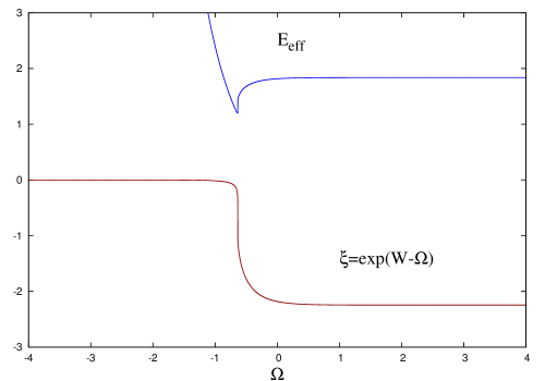
Figure 1: The solution $\xi(\Omega)$ of the algebraic equation (4.32) for $c_{3}=1$, $c_{4}=0.3$, $\eta=1$, $\rho_{g}=0.25\times e^{-4\Omega}+0.25\times e^{-3\Omega}$, $\rho_{f}=0$, and the corresponding potential $E_{\rm eff}(\Omega)$ in (4.34).

If one requires the graviton mass contribution to the total energy density, $\Lambda_{g}$, to be dominant at late times (accelerating phase) but small at early times (matter dominated phase), then one has to have Volkov (2012c)

$$\xi(\Omega)={e^{\cal W}/e^{\Omega}}\to 0~{}~{}{\rm as}~{}~{}~{}e^{\Omega}\to 0\,,$$ (4.35)

as well as

$$b_{1}<0\,.$$ (4.36)

The function $\xi(\Omega)$ is then always negative.

An example of a self-accelerating solution is shown in Fig.1. For $\Omega\to\infty$ one has

$$\xi(\Omega)\to-2.245,~{}~{}~{}~{}~{}~{}E_{\rm eff}(\Omega)\to H=1.837\,,$$ (4.37)

where $H$ is the Hubble expansion rate. In Section V we shall study more general solutions with exactly the same late-time behavior.

(ii) Anisotropic solutions.– If ${\cal S}^{2}=\sigma^{2}C^{2}\neq 0$, then combining (4.28) with (4.25) gives

$$\dot{\Omega}e^{-2\Omega}=C^{2}\dot{\cal W}e^{-2\Omega}\,,$$ (4.38)

from which, denoting the integration constant by $\nu$, we find

$$\xi=\pm\frac{C}{\sqrt{1-\nu e^{2\Omega}}}\,.$$ (4.39)

If $\nu$ does not vanish, then

$${\cal E}=3\nu\sigma^{2}e^{-4\Omega}\left(2-\nu e^{2\Omega}\right)\,.$$

Inserting this to (4.32) gives an algebraic relation between $\xi$ and $\Omega$, which, in view of (4.39), becomes a relation between $\Omega$ and $C$. As a result, $\Omega$ should be constant and no dynamical solutions exist in this case.

If $\nu=0$ then $\xi=C$ and Eq.(4.25) gives ${\cal A}=C\alpha$ so that the two metrics are proportional,

$$f_{\mu\nu}=C^{2}g_{\mu\nu},$$ (4.40)

and ${\cal E}=0$. This case was discussed above in Section IV.1, where we saw that the matter sources should be fine-tuned, $\rho_{g}=C^{2}\rho_{f}$.

IV.2.2 Special solutions

Let us now consider the case where the second factor in (4.27) vanishes,

$$b_{3}\xi^{2}+2b_{2}\xi+b_{1}=0,$$ (4.41)

implying that $\xi$ is constant. Since it should be real, one has to have $b_{2}^{2}-b_{1}b_{3}\geq 0$. The equations to be solved are again (4.30) and (4.31), where now $\dot{\cal W}=\dot{\Omega}$. One has either $\sigma^{2}={\cal S}^{2}=0$ in the isotropic case or, in view of (4.25),

$${\cal A}=\frac{\xi^{3}}{C^{2}}\,\alpha\,,$$ (4.42)

in the anisotropic case. In both cases, taking the difference of (4.30) and (4.31) gives

$${\cal A}=\sqrt{\frac{\Lambda_{g}(\xi)+\rho_{g}}{\Lambda_{f}(\xi)+\rho_{f}}}\,\alpha\,.$$ (4.43)

In the isotropic case this completes the procedure – solution for $g_{\mu\nu}$ is the same as in General Relativity with the cosmological constant $\Lambda_{g}(\xi)$ and matter $\rho_{g}$. The second metric is obtained using the values of $e^{\cal W}=\xi e^{\Omega}$ and of ${\cal A}$ from (4.41),(4.43). The solution exists if only the argument of the square root in (4.43) is positive, which condition turns out to be rather restrictive. For example, if the parameters $b_{k}$ are chosen according (II), then one finds

$$\frac{\Lambda_{g}(\xi)}{\cos^{2}\eta}+\xi^{2}\frac{\Lambda_{f}(\xi)}{\sin^{2}\eta}=-(1-\xi)^{2}\,,$$ (4.44)

so that if $\Lambda_{g}>0$ then $\Lambda_{f}<0$, therefore only solutions with $\rho_{f}>-\Lambda_{f}$ are allowed.

For anisotropic solutions Eqs.(4.42) and (4.43) give

$$C^{2}=\xi^{3}\sqrt{\frac{\Lambda_{f}(\xi)+\rho_{f}}{\Lambda_{g}(\xi)+\rho_{g}}}\,.$$ (4.45)

The argument of the square root here should be positive and, in addition, constant. Since, by our assumption, $\rho_{g},\rho_{f}$ do not contain constant contributions, they should be proportional, $\rho_{f}=(\Lambda_{f}/\Lambda_{g})\rho_{g}$. This excludes self-accelerating solutions with $\Lambda_{g}>0$, since if $\Lambda_{g}$ and $\rho_{g}$ are positive, then both $\Lambda_{f}$ and $\rho_{f}$ are negative and the argument of the square root is negative.

V More general Bianchi types

For the general Bianchi class A models we choose

$$ds_{g}^{2}= - \alpha(t)^{2}dt^{2}+\sum_{a=1,2,3}\alpha^{2}_{a}(t)\,\omega^{a}\otimes\omega^{a}\,,$$

$$ds_{f}^{2}= - {\cal A}(t)^{2}dt^{2}+\sum_{a=1,2,3}{\cal A}^{2}_{a}(t)\,\omega^{a}\otimes\omega^{a}\,,$$ (5.46)

where the vectors dual to $\omega^{a}$ do not commute, so that the spatial curvature do not vanish. Few solutions then can be found in a closed form.

V.0.1 Recovering General Relativity

Assuming again the two metrics and their sources to be proportional, $f_{\mu\nu}=C^{2}g_{\mu\nu}$, we obtain the GR equations,

$$\dot{\Omega}^{2} = \dot{\beta}_{+}^{2}+\dot{\beta}_{-}^{2}-\frac{1}{6}\,\overset{\tiny(3)}{R}+\frac{\Lambda_{g}+\rho}{3}\,,$$ (5.47)

$$\left(e^{3\Omega}\dot{\beta}_{\pm}\right)^{\cdot} = \frac{e^{3\Omega}}{12}\frac{\partial\overset{\tiny(3)}{R}}{\partial\beta_{\pm}}\,,$$ (5.48)

with $\overset{\tiny(3)}{R}$ given by (3.16) and $\Lambda_{g},C$ defined by (IV.1),(4.8). One can choose $C=1$, in which case $\Lambda_{g}=0$.

One cannot integrate the equations for $\beta_{\pm}$ analytically, unless one assumes that $\beta_{\pm}=0$, which is however consistent with (5.48) only when $n^{(1)}=n^{(2)}=n^{(3)}\equiv k$, which corresponds to the Bianchi I,IX for $k=0,1$, respectively. Eq.(5.47) then becomes

$$\dot{\Omega}^{2}=-\frac{k}{4}\,e^{-2\Omega}+\frac{\Lambda_{g}+\rho}{3},$$ (5.49)

which describes the spatially flat $(k=0)$ or spatially closed $(k=1)$ FLRW universe.

V.0.2 The isotropic case

If the the anisotropies vanish but the metrics and their sources are not proportional, then instead of (5.49) one obtains

$$\dot{\Omega}^{2}=-\frac{k}{4}\,e^{-2\Omega}+E^{2}_{\rm eff}(\Omega)\,,$$ (5.50)

where $E_{\rm eff}(\Omega)$ is the same as in (4.34). It is instructive to rewrite this equation as

$$\dot{\bf a}^{2}+V({\bf a})=-k$$ (5.51)

with ${\bf a}=2e^{\Omega}$ and $V=-{\bf a}^{2}E^{2}_{\rm eff}$. Since $\dot{\bf a}^{2}>0$, the solution is restricted to the regions where

$$V({\bf a})\leq-k\,.$$ (5.52)

                 

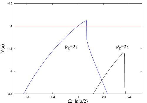
Figure 2: Potential $V({\bf a})$ in (5.51) for isotropic solutions for different choices of the matter density: $\rho_{1}=0.1\times e^{-4\Omega}$ and $\rho_{2}=0.25\times e^{-4\Omega}+0.25\times e^{-3\Omega}$ and $\rho_{f}=0$. In the Bianchi IX case the motion is restricted to the region $V<-1$, so that for $\rho_{g}=\rho_{1}$ one has a recollapsing solution corresponding to the region on the left from the barrier, and a bounce solution corresponding to the region on the right.

To construct $V({\bf a})$ one should resolve the algebraic equation (4.32) (with ${\cal E}=0$) to obtain $\xi(\Omega)$ for chosen $\rho_{g},\rho_{f}$, and then insert the result to (4.34) to obtain $E_{\rm eff}(\Omega)$. In Fig.2 the result is shown for two different choices of $\rho_{g}$ and for $\rho_{f}=0$. One can see that, since $V<0$, for $k=0$ (Bianchi I) the motion covers the whole region ${\bf a}\geq 0$, including the initial singularity at ${\bf a}=0$. The universe therefore expands forever starting from zero size.

The same is true for $k=1$ (Bianchi IX), but if only $\rho_{g}$ is large enough ($\rho_{g}=\rho_{2}$), so that the total amount of matter in the universe is sufficient. If $\rho_{g}$ is small ($\rho_{g}=\rho_{1}$) then the total ‘energy’ is not enough to pass over the barrier, and the motion is divided into two regions. The region on the left from the barrier corresponds to universes which start at the singularity, then expand up to a maximal size, reflect from the barrier, and recollapse. The region on the right from the barrier describe universes that shrink from infinity down to a minimal non-zero size, then bounce from the barrier and expand again to infinity. As we shall see later, these features apply also when the anisotropies are taken into account.

V.1 Generic solutions – integration procedure

As we have seen, exact solutions can be found either in the isotropic case of the Bianchi I and IX, or when the anisotropies are equal, uniquely for the Bianchi I. In all other cases we are bound to use the numerical analysis. Our proceure will be described below, while its outcome can be summarized already now: it turns out that the solutions with equal anisotropies in the two sectors play the role of asymptotic states to which the spacetime approaches at late times.

In order to integrate the equations numerically, we first of all convert the equations to the form of a dynamical system. Let us introduce the variables

$$y_{0} = e^{\Omega},~{}~{}~{}~{}~{}~{}~{}y_{1}=e^{\beta_{+}},~{}~{}~{}~{}~{}~{}~{}y_{2}=e^{\sqrt{3}\beta_{-}},$$ (5.53)

$$y_{3} = e^{\cal W},~{}~{}~{}~{}~{}~{}~{}y_{4}=e^{{\cal B}_{+}},~{}~{}~{}~{}~{}~{}~{}y_{5}=e^{\sqrt{3}{\cal B}_{-}},$$

$$y_{6} = \frac{e^{3\Omega}}{\alpha}\,\dot{\Omega},~{}~{}~{}~{}y_{7}=\frac{e^{3\Omega}}{\alpha}\,\dot{\beta}_{+},~{}~{}~{}y_{8}=\frac{e^{3\Omega}}{\alpha}\,\dot{\beta}_{-},~{}$$

$$y_{9} = \frac{e^{3{\cal W}}}{\cal A}\,\dot{{\cal W}},~{}~{}~{}~{}y_{10}=\frac{e^{3{\cal W}}}{\cal A}\,\dot{{\cal B}}_{+},~{}~{}~{}y_{11}=\frac{e^{3{\cal W}}}{\cal A}\,\dot{{\cal B}}_{-}.$$

The second order field equations (3.18), (3.19), (3.21), (3.22) can be represented in the first order form

$$\dot{y}_{N}=F_{N}(\alpha,{\cal A},y_{M})\,,$$ (5.54)

where $N,M=0,\ldots,11$ and $F_{N}(\alpha,{\cal A},y_{M})$ are defined in the Appendix.

The first order equations (3.17), (3.20), (3.24) are constraints

$${\cal C}_{1}(y_{N})=0,~{}~{}~{}{\cal C}_{2}(y_{N})=0,~{}~{}~{}{\cal C}_{3}(y_{N})=0,~{}~{}~{}$$ (5.55)

with

$${\cal C}_{1} = -y_{6}^{2}+y_{7}^{2}+y_{8}^{2}+2c^{2}y_{0}^{3}U_{g}-\frac{1}{6}\,y_{0}^{6}\,\overset{\tiny(3)}{R}+\frac{1}{3}y_{0}^{6}\,\rho_{g},~{}~{}~{}$$

$${\cal C}_{2} = -y_{9}^{2}+y_{10}^{2}+y_{11}^{2}+2s^{2}y_{3}^{3}{\cal U}_{f}-\frac{1}{6}\,y_{3}^{6}\,\overset{\tiny(3)}{\cal R}+\frac{1}{3}y_{3}^{6}\,\rho_{f},$$

$${\cal C}_{3} = y_{3}^{3}\left(y_{6}y_{0}\frac{\partial}{\partial y_{0}}+y_{7}y_{1}\frac{\partial}{\partial y_{1}}+\sqrt{3}y_{8}y_{2}\frac{\partial}{\partial y_{2}}\right){\cal U}_{f}$$

$$- y_{0}^{3}\left(y_{9}y_{3}\frac{\partial}{\partial y_{3}}+y_{10}y_{4}\frac{\partial}{\partial y_{4}}+\sqrt{3}y_{11}y_{5}\frac{\partial}{\partial y_{5}}\right)U_{g},$$

where $U_{g}$, ${\cal U}_{f}$, $\overset{\tiny(3)}{R}$, $\overset{\tiny(3)}{\cal R}$, $\rho_{g}$, $\rho_{f}$ are defined in the Appendix.

In order to implement the constraints and also determine the lapses $\alpha$ and ${\cal A}$, we remember that the third constraint in (5.55) is obtained as the condition of propagation of the first two. Specifically, calculating the derivatives

$$\dot{\cal C}_{1}=\sum_{N=0}^{11}\frac{\partial{\cal C}_{1}}{\partial y_{N}}\,F_{N}\,,~{}~{}~{}~{}~{}\dot{\cal C}_{2}=\sum_{N=0}^{11}\frac{\partial{\cal C}_{2}}{\partial y_{N}}\,F_{N}\,$$ (5.56)

gives expressions proportional to ${\cal C}_{3}$. Therefore, if the third constraint is fulfilled, ${\cal C}_{3}=0$, then $\dot{\cal C}_{1}=\dot{\cal C}_{2}=0$, so that it is sufficient to require ${\cal C}_{1}={\cal C}_{2}=0$ only at the initial moment of time.

Now, what guarantees that the third constraint propagates itself ? In fact, calculating its time derivative

$$\dot{\cal C}_{3}=\sum_{N=0}^{11}\frac{\partial{\cal C}_{3}}{\partial y_{N}}\,F_{N}\,,$$ (5.57)

and setting the result to zero we discover a non-trivial relation of the form

$$\alpha X_{\alpha}+{\cal A}X_{\cal A}=0,$$ (5.58)

where $X_{\alpha}$ and $X_{\cal A}$ are rather complicated functions of $y_{N}$ (we do not show them explicitly). This is the condition of propagation of the third constraint, which in turn guarantees that the first two constraints propagate. This condition determines the lapse ${\cal A}$,

$${\cal A}=-\frac{X_{\alpha}}{X_{\cal A}}\,\alpha\,.$$ (5.59)

Our procedure is then as follows: we integrate the 12 equations (5.54) with ${\cal A}$ determined by (5.59), where we can use the gauge condition

$$\alpha=1.$$ (5.60)

The three constraints are imposed at the initial time moment, and the above consideration guarantee that they are fulfilled for all times.

To determine the initial data, we choose 9 out of 12 amplitudes $y_{N}$ and give them some initial values. It is convenient to choose

$$y_{0},~{}~{}y_{1},~{}~{}y_{2},~{}~{}y_{4},~{}~{}y_{5},~{}~{}y_{7},~{}~{}y_{8},~{}~{}y_{10},~{}~{}y_{11}$$ (5.61)

which determine $\Omega$, $\beta_{\pm}$, ${\cal B}_{\pm}$, $\dot{\beta}_{\pm}$, $\dot{B}_{\pm}$ at $t=0$. Having chosen these 9 values, the values of $y_{3},y_{6},y_{9}$ determining ${\cal W},\dot{\Omega},\dot{W}$ are obtained by numerically solving the three constraint equations (5.55). Having done these, all initial data are determined, and there remains just to integrate forward the 12 equations (5.54) using the numerical routines of Press et al. (2007).

To check our procedure, we specialize to the Bianchi I type by setting in the equations $n^{(1)}=n^{(2)}=n^{(3)}=0$ and also switch off the matter, $\rho_{g}=\rho_{f}=0$. We then first consider the case where all anisotropies and their time derivatives initially vanish,

$$y_{1}=y_{2}=y_{4}=y_{5}=1\,,~{}~{}y_{7}=y_{8}=y_{10}=y_{11}=0.$$

The numerical integration then reproduces the de Sitter solution, for which these conditions are preserved for all times. Next, if we initially set

$$y_{1}=y_{4}\neq 1,~{}~{}~{}y_{2}=y_{5}\neq 1,~{}~{}~{}y_{7}=y_{8}=y_{10}=y_{11}=0,$$

then these conditions are also preserved for all times. This corresponds to the solution with $\sigma_{\pm}={\cal S}_{\pm}=0$ but with constant values of $\beta_{+}={\cal B}_{+}$ and $\beta_{-}={\cal B}_{-}$. This is again the de Sitter solution, since constant anisotropies can be removed by rescaling the spatial coordinates.

As the next step, we initially choose

$$y_{1} = y_{4}\neq 1,~{}~{}~{}y_{2}=y_{5}\neq 1,~{}~{}~{}y_{7}=\sigma_{+},~{}~{}y_{8}=\sigma_{-},$$

$$y_{10} = C\sigma_{+},~{}~{}~{}y_{11}=C\sigma_{-},~{}~{}~{}~{}C={y_{3}^{3}}/{({\cal A}y_{0}^{3})}\,.$$ (5.62)

The numerical solution then again preserves these conditions at all times, which corresponds to the analytic solutions with equal anisotropies.

V.2 Numerical results

After consistency checks, we turn to the generic case. We switch on the matter by setting in the equations $\rho_{g}\neq 0$ and $\rho_{f}\neq 0$. We choose an initial value for $y_{0}=e^{\Omega}$ and some values for $y_{1}=e^{\beta_{+}}$, $y_{2}=e^{\sqrt{3}\beta_{-}}$, $y_{3}=e^{{\cal B}_{+}}$, $y_{4}=e^{\sqrt{3}{\cal B}_{-}}$ assuming that $\beta_{\pm}$ and ${\cal B}_{\pm}$ are not too large. In addition, we choose small enough values for $y_{7},y_{8},y_{10},y_{11}$ determining $\dot{\beta}_{\pm}$, $\dot{\cal B}_{\pm}$, so that the initial configuration is not too anisotropic.

We consider all Bianchi class A types. The values of the parameters $n^{(a)}$ are given in Table I.

	I	II	VI0	VII0	VIII	IX
$n^{(1)}$	$0$	$1$	$1$	$1$	$1$	$1$
$n^{(2)}$	$0$	$0$	$-1$	$1$	$1$	$1$
$n^{(3)}$	$0$	$0$	$0$	$0$	$-1$	$1$

Table 1: Values of $n^{(a)}$ for Bianchi class A types

We find that if the parameters are chosen such that the universe enters the self-accelerating regime, then generic solutions rapidly approach the state with equal and constant anisotropies, $\beta_{+}={\cal B}_{+}$ and $\beta_{-}={\cal B}_{-}$. For Bianchi I type one can scale away these constant values by rescaling the spatial coordinates, but this cannot be done for other Bianchi types. As a result, the final state of the universe is anisotropic, even though the metric amplitudes $\dot{\Omega}$, $\dot{\cal W}$, ${\cal A}$ approach constant values, as for the isotropic universe.

   

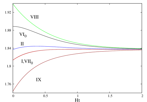
Figure 3: The Hubble parameter $\dot{\Omega}$ for solution for all Bianchi types of class A.

Some examples of our solutions are presented in Figs.3–9 for the parameter values $c_{3}=1$, $c_{4}=0.3$, $\eta=1$, which are the same as for the FLRW self-accelerating solution in Fig.1. We assume the f-sector to be empty, while the g-sector to contain a radiation and a non-relativistic matter described by $\rho_{g}=0.25\times e^{-4\Omega}+0.25\times e^{-3\Omega}\,,$ which is the same function as in Figs.1,2. There is nothing special about this choice, since for other parameter values solutions are qualitatively the same. (We notice that $\rho_{g}\sim 1$ for $\Omega=0$, therefore, if $m\sim 10^{-33}{\rm eV}$, the dimensionful energy density in (II.1) is $\sim m^{2}/\kappa^{2}\sim 10^{-10}({\rm eV})^{4}$, which is about the present density of the universe). The universe will accelerate if $c_{3},c_{4}$ are chosen such that $b_{1}<0$ (see Eq.(4.36)) while $\rho_{g}$ is large enough in order that the system could travel over the potential barrier as shown in Fig.2. It is also worth noting that the time scale in Figs.3–9 is the Hubble time, $1/H$.

   

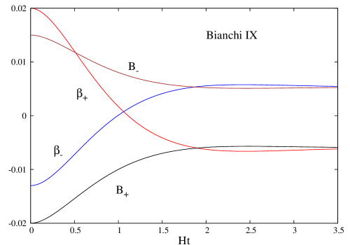
Figure 4: Anisotropy amplitudes profiles for Bianchi IX. For other Bianchi types the picture is similar.

The initial value of the scale factor is $\Omega=0$ and the initial anisotropies are $\beta_{+}=0.02$, $\beta_{-}=-0.013$, ${\cal B}_{+}=-0.02$, ${\cal B}_{-}=0.015$, while the initial values of $\dot{\beta}_{\pm}$, $\dot{\cal B}_{\pm}$ are set to zero. Again, changing these values does not change the qualitative behavior of the solutions. The values of ${\cal W}$, $\dot{\Omega}$, $\dot{\cal W}$ are determined by the constraints (5.55).

   

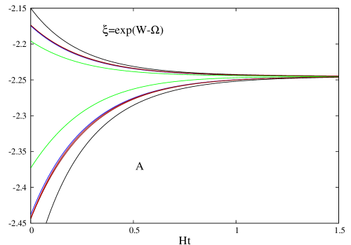
Figure 5: The ratio of the two scale factors $\xi=e^{{\cal W}-\Omega}$ and the lapse amplitude ${\cal A}$ for all Bianchi types.

As seen in Fig.3, for all Bianchi types the universe expansion rate rapidly approaches the constant value, $\dot{\Omega}\to H=1.837$ (the same value as in Eq.(4.18)), so that the universe approaches the de Sitter phase. If we return for a moment to dimensionful quantities, the Hubble rate becomes ${\bf H}=Hm$, so that the cosmological constant is indeed due to the graviton mass.

   

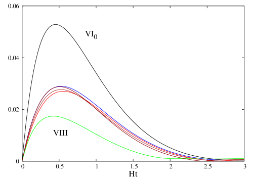
Figure 6: The relative magnitude of shears $\Sigma=(\dot{\beta}_{+}^{2}+\dot{\beta}_{-}^{2})^{1/2}/\dot{\Omega}$ for all Bianchi types.

The anisotropy amplitudes $\beta_{\pm}$, ${\cal B}_{\pm}$ approach constant values within an approximately twice Hubble time, $2H^{-1}$, as is seen in Fig.4, where the solutions for the Bianchi IX are shown. The ratio of the two scale factors $\xi=e^{\cal W}/e^{\Omega}$ is shown in Fig.5. It is always negative for all solutions and rapidly approaches the value $C=-2.245$, which is the same as in Eq.(4.16). The lapse function ${\cal A}$, also shown in Fig.6, approaches the same value, so that the two metrics become proportional at late times, $f_{\mu\nu}=C^{2}g_{\mu\nu}$, as for the solutions in section IV.1.

Fig.6 shows the relative magnitude of shears

$$\Sigma={(\dot{\beta}_{+}^{2}+\dot{\beta}_{-}^{2})^{1/2}\over\dot{\Omega}}\,,$$

which measures the relative contribution of the anisotropies to the total expansion rate. The maximal value of $\Sigma$ depends on the initial anisotropy values. However, setting the latter to zero we obtain practically the same curves for the Bianchi types II,VI₀,VII₀,VIII, since anisotropies cannot be zero in these cases, so that they are driven to non-zero values by the cosmic expansion. The shears approach zero exponentially fast in Hubble units. However, if our universe entered the acceleration phase only recently, then one can expect that only few e-folding times have elapsed since then, so that the shear energy is not necessarily small at present.

   

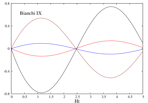
Figure 7: The rescaled shears $e^{3\Omega/2}\dot{\beta}_{\pm}$ (smaller amplitudes) and $e^{3\Omega/2}\dot{\cal B}_{\pm}$ (larger amplitudes) for the Bianchi IX solution, for other Bianchi types the picture is similar.

The shears $\dot{\beta}_{\pm}$, $\dot{\cal B}_{\pm}$ multiplied by $e^{3\Omega/2}$ oscillate with constant amplitudes, as shown in Fig.7, so that $\dot{\beta}_{\pm}\sim\dot{\cal B}_{\pm}\sim e^{-3\Omega/2}$. To understand this, we remember that our configurations approach the solution with proportional metrics, $f_{\mu\nu}=C^{2}g_{\mu\nu}$, described in section IV.1, so that the deviations from this solutions are small at late times. We therefore linearize the field equations with respect to the deviations, and solving the linearized equations we obtain

$$\dot{\beta}_{\pm}\sim\dot{\cal B}_{\pm}\sim e^{-3Ht/2}\cos(H\omega t)$$ (5.63)

with

$$\omega^{2}=(b_{1}+2Cb_{2}+C^{2}b_{3})\left(\frac{C\cos^{2}\eta}{H^{2}}+\frac{\sin^{2}\eta}{CH^{2}}\right)-\frac{9}{4}\,.$$ (5.64)

For our parameter values this gives $\omega=1.183$ and the oscillation period in Hubble time units $T=2\pi/\omega=5.309$, in perfect agreement with what is shown in Fig.7.

Therefore, the shear contribution to the Hubble rate is

$$\dot{\beta}_{+}^{2}+\dot{\beta}_{-}^{2}\sim e^{-3\Omega}\sim 1/{\bf a}^{3}\,,$$ (5.65)

which falls off similarly to the energy density of a non-relativistic matter. In GR (see the Appendix) the shear falloff is much faster, $\dot{\beta}_{+}^{2}+\dot{\beta}_{-}^{2}\sim 1/{\bf a}^{6}$, corresponding to a ‘stiff matter’. Since in the bigravity the shear contribution to the total energy density increases slowly, this could have observational effects.

V.2.1 Near singularity behavior

It is interesting to see how the solutions continue to the past. Their parameters are chosen to avoid the bounce behavior, so that when continued to the negative $t$ region, they should hit a singularity at some point. The numerical simulations confirm these expectations and reveal that for all Bianchi types under consideration there is a singularity for $t<0$, where both $e^{\Omega}$ and $e^{\cal W}$ vanish. For the Bianchi I this is shown in Fig.8.

   

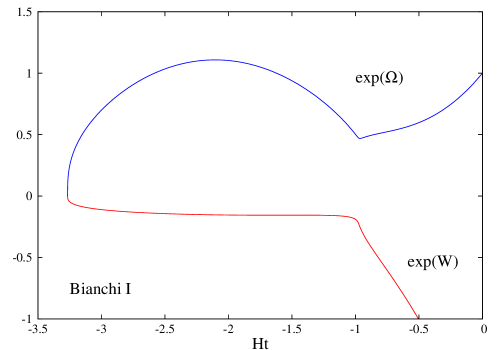
Figure 8: The scale factors near the singularity.

Interestingly, in the negative $t$ region the solution shows a throat, and $e^{\Omega}$ first expands before collapsing to zero.

Let us consider in more detail the case of Bianchi IX. In General Relativity Bianchi IX solutions reveal chaotic features. When approaching singularity, the metric coefficients $\alpha_{a}$ which measure the proper distances along the spatial axes (defined in (3.13)) show an infinite number of oscillations, whose positions and amplitudes are ergodic Misner (1969); *Belinskii:1972. Within an effective description, such a behavior is explained by a two dimensional ‘billiard’ motion of a particle reflecting from rigid walls.

   

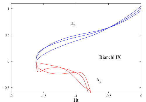
Figure 9: The metric coefficients $\alpha_{a}$, ${\cal A}_{a}$ near the singularity.

At first glance, nothing similar is seen in our case. Fig.9 shows the Bianchi IX solution continued to the past, and the singularity corresponds to a point where both $e^{\Omega}$ and $e^{\cal W}$ vanish, but in its vicinity coefficients $\alpha_{a}$, ${\cal A}_{a}$ defined by (3.13) approach zero without oscillations. However, zooming the picture one can see that oscillations actually start, but not many of them are seen, since we cannot approach the singularity close enough due to numerical errors.

   

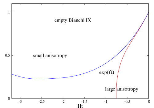
Figure 10: Self-accelerating for $t>0$ Bianchi IX solutions continued to the $t<0$ region. Choosing at $t=0$ $\beta_{\pm}\sim{\cal B}_{\pm}\sim 10^{-2}$, the solution is of regular bounce type, but if $\beta_{\pm}\sim{\cal B}_{\pm}\sim 10^{-1}$ then the solution develops a singularity where $e^{\Omega}$ vanishes.

The picture becomes more clear for solutions without matter. Setting $\rho_{g}=\rho_{f}=0$, the simplest salf-accelerating solution is pure de Sitter, but it is of course non-singular. It can be obtained from Eq.(5.51), which reduces to (remember that ${\bf a}=2e^{\Omega}$)

$$\dot{\bf a}^{2}=H^{2}{\bf a}^{2}-1\,~{}~{}~{}~{}\Rightarrow~{}~{}~{}{\bf a}=\frac{1}{H}\,\cosh(t-t_{0}),$$ (5.66)

where $H=1.837$ is the same as for all other solutions under considerations. Qualitatively, the singularity is avoided because ${\bf a}$ cannot be too small, since otherwise the right hand side of the equation would be negative. Therefore, ${\bf a}$ bounces back when it achieves the minimal value $1/H$.

However, for non-zero anisotropy the equation in (5.66) receives in the right hand side additional terms proportional to $\dot{\beta}_{+}^{2}+\dot{\beta}_{-}^{2}$, and these can keep the whole expression on the right positive even if ${\bf a}\to 0$. Therefore, solutions with high enough anisotropy can approach singularity. To verify this, we choose at $t=0$ two sets of initial values for the anisotropies, $\beta_{\pm}\sim{\cal B}_{\pm}\sim 10^{-2}$ and $\beta_{\pm}\sim{\cal B}_{\pm}\sim 10^{-1}$. When continued to the future, we see self-acceleration in both cases, but when continued to the past, we obtain the bounce behavior in the first case and a curvature singularity in the second case (see Fig.10). Therefore, the empty de Sitter spacetime becomes singular when too much anisotropy is added.

It happens that for the empty Bianchi IX solution we can approach the singularity much closer numerically, and in Fig.11 we show $\ln(\alpha_{a})$ against $\Omega\propto\ln(t)$. This time one can clearly see the typical features of the billiard motion characterized by a sequence of Kasner-like periods. During each period one has $\alpha_{a}\propto t^{p_{a}}$, where $p_{a}$ fulfill Eq.(A.1.76). During the next period, the values ${p_{a}}$ change such that one of then remains positive, the corresponding amplitude continues to decrease toward singularity ($\alpha_{3}$ in the Fig.10), while two other $p_{a}$’s change sign, such that the increasing amplitude becomes decreasing and vise versa.

   

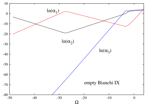
Figure 11: The anisotropy parameters $\alpha_{a}$ for the empty Bianchi IX near the singularity plotted against $\Omega$. They show the typical ‘billiard’ behavior characterized by a sequence of Kasner periods. For ${\cal A}_{a}$ the picture is similar.

Of course, within our numerical approach we can capture only the beginning of the infinite sequence of Kasner-like steps, and so it would be interesting to develop an affective analytical description. If the mater is present, provided that $w<1$, then its contribution to the equations is subleading as compared to that of the anisotropy terms, so that it cannot influence the chaotic behavior. Therefore, since the empty Bianchi IX solutions are chaotic, so should be those with matter.

VI Concluding Remarks

We have studied anisotropic cosmologies in the ghost-free bigravity assuming both metrics to be diagonal and of the same Bianchi type of class A. Including a source consisting of a radiation and a non-relativistic matter, we considered generic initial data describing (not too large) anisotropic deformations of a FLRW universe. We find that the universe evolves into a state in which it expands with a constant Hubble rate proportional to the graviton mass, while the anisotropy parameters approach constant non-zero values. In the Bianchi I case constant anisotropies can be scaled away be redefining the spatial coordinates, but not for other Bianchi types. For example, for the Bianchi IX solutions the constant $t$ spatial sections will be not round 3-spheres but squashed spheres.

The conclusion is that generic self-accelerating cosmologies in bigravity are anisotropic. The anisotropy contribution to the total expansion rate approaches zero exponentially fast in Hubble units, but if our universe entered the acceleration phase only recently, then one can expect that only few e-folding times have elapsed since then, so that the shear energy is not necessarily small. At late times the shear contribution to the total expansion rate decreases much slower than in GR, only as an inverse cube of the size of the universe, which is the same falloff rate as for a non-relativistic matter. Therefore, the anisotropy effect could be visible, although comparing with observations goes beyond the scope of this paper (see Akrami et al. (2013) for a data-fitting for the FLRW cosmologies with massive gravitons).

The fact that the anisotropy contribution shows the same falloff rate as a cold dark matter suggests that the latter could in fact be the effect of the anisotropies. If this were true, then it would follow that theories with massive gravitons could explain both the dark energy – the cosmological term mimicked by the graviton mass, and also the cold dark matter mimicked by the anisotropies. However, it is unclear if this interpretation can explain also the other properties of dark matter, as for example its clustering. In addition, the high isotropy of the cosmic microwave background implies that already at the recombination the metric anisotropies were small, therefore they are unlikely to explain almost a quarter of the total energy in the universe presently attributed to the dark matter. It would nevertheless be interesting to check if the anisotropy energy has a tendency for clustering, which could perhaps be seen at the level of perturbations, but such an analysis requires a separate study.

It would be interesting to develop an analytic description for the behavior of the Bianchi IX solutions near singularity. Yet one more interesting open issue would be to see if the FLRW solutions with non-diagonal metrics studied in Koyama et al. (2011a); *Koyama:2011yg, Chamseddine and Volkov (2011), D’Amico et al. (2011), Kobayashi et al. (2012), Volkov (2012a); *Volkov:2012zb could be generalized for non-zero anisotropies.

Appendix A Bianchi I spacetimes in GR

In this Appendix, we discuss the Bianchi I spacetime in General Relativity for some matter types. Assuming the metric form

$$ds^{2} = -dt^{2}+\sum_{a=1,2,3}\alpha_{a}(t)^{2}(dx^{a})^{2}$$ (A.1.67)

where

$$\alpha_{1}=e^{\Omega}e^{\beta_{+}+\sqrt{3}\beta_{-}}\,,~{}~{}\alpha_{2}=e^{\Omega}e^{\beta_{+}-\sqrt{3}\beta_{-}}\,,~{}~{}\alpha_{3}=e^{\Omega}e^{-2\beta_{+}}\,,$$

the Einstein equations reduce to

$$\left(e^{3\Omega}\,{\dot{\Omega}}\right)^{2} = \left(e^{3\Omega}\,{\dot{\beta}_{+}}\right)^{2}+\left(e^{3\Omega}\,{\dot{\beta}_{-}}\right)^{2}+\frac{1}{3}e^{6\Omega}\rho\,,~{}~{}~{}~{}$$

$$\left(e^{3\Omega}\,{\dot{\Omega}}\right)^{\centerdot} = \frac{1}{2}\,e^{3\Omega}(\rho-P),$$

$$\left(e^{3\Omega}\,{\dot{\beta}_{\pm}}\right)^{\centerdot} = 0,$$ (A.1.68)

where $\rho$ and $P$ are the energy density and pressure, which fulfill the energy conservation condition,

$$\dot{\rho}+3\dot{\Omega}\,(\rho+P)=0.$$ (A.1.69)

The last of Eqs. (A.1.68) can be integrated to give

$$e^{3\Omega}\dot{\beta}_{\pm}=\sigma_{\pm}\,,$$ (A.1.70)

where $\sigma_{\pm}$ are integration constants, from where

$$\beta_{\pm}=\beta_{\pm}(t_{0})+\sigma_{\pm}\int_{t_{0}}^{t}e^{-3\Omega}dt\,.$$ (A.1.71)

The equations then reduce to

$$\left(e^{3\Omega}\,{\dot{\Omega}}\right)^{2}=\sigma^{2}+\frac{1}{3}e^{6\Omega}\rho\,,$$ (A.1.72)

where $\sigma^{2}=\sigma_{-}^{2}+\sigma_{+}^{2}$ and $\rho$ is determined by the energy conservation condition,

$$\rho=\rho_{0}e^{-3(1+w)\Omega}\,,$$ (A.1.73)

assuming the equation of state $P=w\rho$.

A.0.1 Vacuum solutions

Setting in the above formulas $\rho=\rho_{0}=0$, one can integrate Eqs.(A.1.71),(A.1.72) to obtain

$$\alpha_{a}\propto t^{p_{a}}\,,~{}~{}~{}~{}a=1,2,3$$ (A.1.74)

where

$$p_{1} = \frac{1}{3}(1+\frac{\sigma_{+}+\sqrt{3}\sigma_{-}}{\sigma}),~{}~{}~{}p_{2}=\frac{1}{3}(1+\frac{\sigma_{+}-\sqrt{3}\sigma_{-}}{\sigma}),~{}~{}$$

$$p_{3} = \frac{1}{3}(1-2\frac{\sigma_{+}}{\sigma}),$$ (A.1.75)

so that

$$p_{1}+p_{2}+p_{3}=p_{1}^{2}+p_{2}^{2}+p_{3}^{2}=1.$$ (A.1.76)

This corresponds to the Kasner solution.

A.0.2 Cosmological constant

Let us choose in (A.1.73) $w=-1$ and $\rho=\rho_{0}=3H^{2}$. The solution of (A.1.72) is then

$$e^{3\Omega}=e^{3H(t-t_{0})}-\frac{\sigma^{2}e^{-3H(t-t_{0})}}{4H^{2}}.$$ (A.1.77)

Inserting this to (A.1.71) determines $\beta_{\pm}$. If $\sigma_{\pm}=0$ then the solution is pure de Sitter, $\Omega=H(t-t_{0})$, with constant anisotropy parameters $\beta_{\pm}$ which can be set to zero via rescaling the spatial coordinates $x^{a}$. If $\sigma_{\pm}\neq 0$, then the solution approaches the de Sitter metric exponentially fast,

$$\Omega=H(t-t_{0})+O(e^{-3Ht}),~{}~{}~{}~{}\beta_{\pm}=\beta_{\pm}(\infty)+O(e^{-3Ht})\,.$$ (A.1.78)

Calculating the integral in (A.1.71) gives explicitly

$$\alpha_{a}\propto e^{Ht}X_{+}^{2/3}\left(\frac{X_{-}}{X_{+}}\right)^{p_{a}}\,,~{}~{}~{}~{}a=1,2,3,$$ (A.1.79)

where $p_{a}$ are the same as in (A.0.1) and

$$X_{\pm}=1\pm\frac{\sigma}{2H}\,e^{-3H(t-t_{0})}.$$ (A.1.80)

One has $X_{\pm}\to 1$ as $t\to\infty$, so that solutions approach de Sitter metric. On the other hand, taking the limit $H\to 0$ and choosing the integration constant $t_{0}$ such that $\sigma/(2H)e^{3Ht_{0}}=1$ one has $X_{+}\to 2$ and $X_{-}\to 3Ht$ in this limit, and therefore $\alpha_{a}\propto t^{p_{a}}$, so that the Kasner solution is recovered.

One can similarly obtain solutions for a negative cosmological constant, when $w=-1$ and $\rho=\rho_{0}=-3H^{2}$. The solution of (A.1.72) is then

$$e^{3\Omega}=\frac{\sigma}{H}\,\sin(3H(t-t_{0}))\,,$$ (A.1.81)

inserting which to (A.1.71) gives

$$\alpha_{a}\propto\left(\cos\frac{3H(t-t_{0})}{2}\right)^{2/3}\left(\tan\frac{3H(t-t_{0})}{2}\right)^{p_{a}}\,,$$ (A.1.82)

where $p_{a}$ are again the same as in (A.0.1).

A.0.3 More general matter

For a general equation of state Eq.(A.1.72) reduces to

$$\left(e^{3\Omega}\,{\dot{\Omega}}\right)^{2}=\sigma^{2}+\frac{\rho_{0}}{3}e^{3\Omega(1-w)}\,,$$ (A.1.83)

which shows that the anisotropy contribution always becomes small for large $\Omega$, provided that $w<1$. This equation can be integrated in quadratures, the late time behavior of the solution is

$$e^{3\Omega}\sim t^{\frac{2}{w+1}},~{}~{}~{}~{}\beta=\beta(\infty)+O(t^{\frac{w-1}{w+1}}).$$ (A.1.84)

One can also consider a more general matter consisting of several components with different equations of state, $P_{i}=w_{i}\rho_{i}$, in which case

$$\rho=\sum_{i}\rho_{i0}e^{-3(1+w_{i})\Omega}\,.$$ (A.1.85)

For example, if there is a cosmological constant plus a one-component perfect fluid, then Eq.(A.1.72) reduces to

$$\left(e^{3\Omega}\,{\dot{\Omega}}\right)^{2}=\sigma^{2}+H^{2}e^{6\Omega}+\frac{\rho_{0}}{3}e^{3\Omega(1-w)}\,.$$ (A.1.86)

If $w>-1$ then for large $\Omega$ the second term on the right becomes dominant and the universe approaches the de Sitter state. The conclusion is that in all cases the anisotropy effect soon becomes negligible when the universe expands.

Appendix B Dynamical system description

The second order equations (3.18), (3.19), (3.21), (3.22) can be represented in the first order form

$$\dot{y}_{N}=F_{N}(\alpha,{\cal A},y_{M}),$$ (A.2.87)

where the variables $y_{N}(t)$ are defined in (5.53), while

$$F_{0} = \alpha\,\frac{y_{6}}{y_{0}^{2}}\,,~{}~{}~{}F_{1}=\alpha\,\frac{y_{1}y_{7}}{y_{0}^{3}}\,,~{}~{}~{}F_{2}=\sqrt{3}\,\alpha\,\frac{y_{2}y_{8}}{y_{0}^{3}}\,,~{}~{}~{}F_{3}={\cal A}\,\frac{y_{9}}{y_{3}^{2}}\,,~{}~{}~{}~{}F_{4}={\cal A}\,\frac{y_{4}y_{10}}{y_{3}^{3}}\,,~{}~{}~{}F_{5}=\sqrt{3}\,{\cal A}\,\frac{y_{5}y_{11}}{y_{3}^{3}},$$

$$F_{6} = {1\over 6}\left[\cos^{2}\eta\left(y_{0}\frac{\partial U}{\partial y_{0}}+3\alpha U_{g}\right)+3{\alpha}\,y_{0}^{3}\,(\rho_{g}-P_{g})-2{\alpha}\,y_{0}^{3}\,\overset{\tiny(3)}{R}\right]\,,~{}~{}~{}F_{7}={1\over 12}\left[-2\,{\cos^{2}\eta}\,y_{1}\frac{\partial U}{\partial y_{1}}+{\alpha}\,y_{0}^{3}\,y_{1}\frac{\partial\overset{\tiny(3)}{R}}{\partial y_{1}}\right]\,,~{}~{}~{}~{}~{}~{}~{}$$

$$F_{8} = {\sqrt{3}\over 12}\left[-2\,{\cos^{2}\eta}\,y_{2}\frac{\partial U}{\partial y_{2}}+{\alpha}\,y_{0}^{3}\,y_{2}\frac{\partial\overset{\tiny(3)}{R}}{\partial y_{2}}\right]\,,~{}~{}~{}F_{9}={1\over 6}\left[{\sin^{2}\eta}\,\left(y_{3}\frac{\partial U}{\partial y_{3}}+3{\cal A}\,{\cal U}_{f}\right)+3{\cal A}\,y_{3}^{3}\,(\rho_{f}-P_{f})-2{\cal A}\,y_{3}^{3}\,\overset{\tiny(3)}{\cal R}\right]\,,~{}~{}~{}$$

$$F_{10} = {1\over 12}\left[-2\sin^{2}\eta\,y_{4}\frac{\partial U}{\partial y_{4}}+{\cal A}\,y_{3}^{3}\,y_{4}\frac{\partial\overset{\tiny(3)}{R}}{\partial y_{4}}\right]\,,~{}~{}~{}F_{11}={\sqrt{3}\over 12}\left[-2\,{\sin^{2}\eta}\,y_{5}\frac{\partial U}{\partial y_{5}}+{\cal A}\,y_{3}^{3}\,y_{5}\frac{\partial\overset{\tiny(3)}{R}}{\partial y_{5}}\right]\,.$$

Here $U=\alpha\,U_{g}+{\cal A}\,{\cal U}_{f}$ with

$$U_{g} = y_{0}^{3}\{b_{0}+b_{1}(\lambda_{1}+\lambda_{2}+\lambda_{3})+b_{2}(\lambda_{1}\lambda_{2}+\lambda_{1}\lambda_{3}+\lambda_{2}\lambda_{3})+b_{3}\lambda_{1}\lambda_{2}\lambda_{3}\}$$

and ${\cal U}_{f}$ is obtained from $U_{g}$ by replacing $b_{k}\to b_{k+1}$, where the eigenvalues $\lambda_{i}$ are given by

$$\lambda_{1}=\frac{y_{3}y_{4}y_{5}}{y_{0}y_{1}y_{2}},~{}~{}~{}~{}~{}~{}\lambda_{2}=\frac{y_{3}y_{4}y_{2}}{y_{0}y_{1}y_{5}},~{}~{}~{}~{}~{}\lambda_{3}=\frac{y_{3}y_{1}^{2}}{y_{0}y_{4}^{2}}.$$ (A.2.88)

The 3-curvatures are

$$\overset{\tiny(3)}{R}=\frac{2\,n^{(1)}n^{(3)}\,y_{2}^{2}}{y_{0}^{2}y_{1}^{2}}-\frac{1}{2}\left(\frac{n^{(1)}\,y_{2}^{4}y_{1}^{6}-n^{(2)}\,y_{1}^{6}+n^{(3)}\,y_{2}^{2}}{y_{0}y_{2}^{2}y_{1}^{4}}\right)^{2}\,,~{}~{}$$

while $\overset{\tiny(3)}{\cal R}$ is obtained by replacing in this expression $y_{0}\to y_{3}$, $y_{1}\to y_{4}$, $y_{2}\to y_{5}$. Finally, the matter terms are

$$\rho_{g}=\sum_{i}\rho_{g}^{(i)}y_{0}^{-3(1+w^{(i)}_{g})},~{}~{}~{}P_{g}=\sum_{i}w^{(i)}_{g}\rho_{g}^{(i)}y_{0}^{-3(1+w^{(i)}_{g})},~{}~{}~{}$$ (A.2.89)

where $\rho_{g}^{(i)}$, $w^{(i)}_{g}$ are constant parameters, while $\rho_{f}$, $P_{f}$ are obtained by replacing in these expressions $y_{0}\to y_{3}$ and $\rho_{g}^{(i)}\to\rho_{f}^{(i)}$, $w^{(i)}_{g}\to w^{(i)}_{f}$ (the number of matter components needs not to be the same in both sectors).

References

- de Rham et al. (2011) C. de Rham, G. Gabadadze, and A. J. Tolley, Phys.Rev.Lett. 106, 231101 (2011).
- Hassan and Rosen (2012a) S. Hassan and R. A. Rosen, JHEP 1202, 126 (2012a).
- Fierz and Pauli (1939) M. Fierz and W. Pauli, Proc.Roy.Soc.Lond. A173, 211 (1939).
- Boulware and Deser (1972) D. Boulware and S. Deser, Phys.Rev. D6, 3368 (1972).
- Hassan and Rosen (2012b) S. F. Hassan and R. A. Rosen, Phys.Rev.Lett. 108, 041101 (2012b).
- Golovnev (2012) A. Golovnev, Phys.Lett. B707, 404 (2012).
- Kluson (2012) J. Kluson, Phys.Rev. D86, 044024 (2012).
- Hassan et al. (2012) S. Hassan, A. Schmidt-May, and M. von Strauss, Phys.Lett. B715, 335 (2012).
- Hassan and Rosen (2012c) S. Hassan and R. A. Rosen, JHEP 1204, 123 (2012c).
- Riess et al. (1998) A. G. Riess et al., Astron.Journ. 116, 1009 (1998).
- Perlmutter et al. (1999) S. Perlmutter et al., Astrophys.Journ. 517, 565 (1999).
- Damour et al. (2002) T. Damour, I. I. Kogan, and A. Papazoglou, Phys. Rev. D 66, 104025 (2002).
- Koyama et al. (2011a) K. Koyama, G. Niz, and G. Tasinato, Phys.Rev.Lett. 107, 131101 (2011a).
- Koyama et al. (2011b) K. Koyama, G. Niz, and G. Tasinato, Phys.Rev. D84, 064033 (2011b).
- Chamseddine and Volkov (2011) A. H. Chamseddine and M. S. Volkov, Phys.Lett. B704, 652 (2011).
- D’Amico et al. (2011) G. D’Amico, C. de Rham, S. Dubovsky, G. Gabadadze, D. Pirtskhalava, et al., Phys.Rev. D84, 124046 (2011).
- Kobayashi et al. (2012) T. Kobayashi, M. Siino, M. Yamaguchi, and D. Yoshida, Phys.Rev. D86, 061505 (2012).
- Gratia et al. (2012) P. Gratia, W. Hu, and M. Wyman, Phys.Rev. D86, 061504 (2012).
- Volkov (2012a) M. S. Volkov, Phys.Rev. D86, 061502 (2012a).
- Volkov (2012b) M. S. Volkov, Phys.Rev. D86, 104022 (2012b).
- Gumrukcuoglu et al. (2011) A. E. Gumrukcuoglu, C. Lin, and S. Mukohyama, JCAP 1111, 030 (2011).
- De Felice et al. (2012) A. De Felice, A. E. Gumrukcuoglu, and S. Mukohyama, Phys.Rev.Lett. 109, 171101 (2012).
- Volkov (2012c) M. S. Volkov, JHEP 1201, 035 (2012c).
- von Strauss et al. (2012) M. von Strauss, A. Schmidt-May, J. Enander, E. Mortsell, and S. Hassan, JCAP 1203, 042 (2012).
- Comelli et al. (2012a) D. Comelli, M. Crisostomi, F. Nesti, and L. Pilo, JHEP 1203, 067 (2012a).
- Comelli et al. (2012b) D. Comelli, M. Crisostomi, and L. Pilo, JHEP 1206, 085 (2012b).
- Khosravi et al. (2012) N. Khosravi, H. R. Sepangi, and S. Shahidi, Phys.Rev. D86, 043517 (2012).
- Gumrukcuoglu et al. (2012) A. E. Gumrukcuoglu, C. Lin, and S. Mukohyama, Phys.Lett. B717, 295 (2012).
- Sakakihara et al. (2012) Y. Sakakihara, J. Soda, and T. Takahashi, (2012), arXiv:1211.5976 [hep-th] .
- Starobinsky (1983) A. A. Starobinsky, JETP Lett. 37, 66 (1983).
- Muller et al. (1990) V. Muller, H. Schmidt, and A. A. Starobinsky, Class.Quant.Grav. 7, 1163 (1990).
- Wald (1983) R. M. Wald, Phys.Rev. D28, 2118 (1983).
- Kitada and Maeda (1992) Y. Kitada and K.-i. Maeda, Phys.Rev. D45, 1416 (1992).
- Kitada and Maeda (1993) Y. Kitada and K.-i. Maeda, Class.Quant.Grav. 10, 703 (1993).
- Press et al. (2007) W. H. Press, S. A. Teukolsky, W. T. Vetterling, and B. P. Flannery, Numerical Recipes 3rd Edition: The Art of Scientific Computing, 3rd ed. (Cambridge University Press, New York, NY, USA, 2007).
- Misner (1969) C. W. Misner, Phys. Rev. Lett. 22, 1071 (1969).
- Belinskii et al. (1972a) V. Belinskii, E. Lifshitz, and I. Khalatnikov, Sov.JETP 35, 838 (1972a).
- Belinskii et al. (1972b) V. Belinskii, E.M., and I. Khalatnikov, Sov.JETP 36, 591 (1972b).
- Akrami et al. (2013) Y. Akrami, T. S. Koivisto, and M. Sandstad, (2013), arXiv:1302.5268 [astro-ph.CO] .