Statistical Characterisation & Classification of Edge Localised Plasma Instabilities

Abstract

The statistics of edge-localised plasma instabilities (ELMs) in toroidal magnetically confined fusion plasmas are considered. From first principles, standard experimentally motivated assumptions are shown to determine a specific probability distribution for the waiting times between ELMs: the Weibull distribution. This is confirmed empirically by a statistically rigorous comparison with a large data set from the Joint European Torus (JET). The successful characterisation of ELM waiting times enables future work to progress in various ways. Here we present a quantitative classification of ELM types, complementary to phenomenological approaches. It also informs us about the nature of ELMing processes, such as whether they are random or deterministic.

Introduction: Edge localised plasma instabilities (ELMs) Keilhacker et al. (1984); Zohm (1996); Loarte et al. (2003); Kamiya et al. (2007) are almost ubiquitous in high performance magnetically confined fusion (MCF) plasmas. Their phenomenological properties are correlated with the quality of global energy confinement, and the peak energy fluxes onto material surfaces Loarte et al. (2003); Kamiya et al. (2007); McDonald ; Rapp . Key challenges are to statistically characterise these processes sufficiently well that a quantitative distinction between different observed classes of ELMs becomes possible, and to relate this classification to the physical processes responsible for them. This will provide a test for theoretical models, and is an important step towards improved estimates for the distribution of ELM waiting times and sizes, both of which must be controlled in reactor-scale MCF plasma experiments.

ELMs offer a rich and diverse experimental phenomenology Keilhacker et al. (1984); Zohm (1996); Loarte et al. (2003); Kamiya et al. (2007); McDonald ; Rapp ; Liang ; Degeling . There is intense theoretical research on the instabilities that may be responsible for triggering them Webster , but few unifying principles have been identified. We will show that widely held experimentally motivated assumptions about ELMing require particular statistical characteristics. Specifically, if one assumes that the likelihood of ELM occurrence increases monotonically with time elapsed since the most recent ELM, then the measured distribution of waiting times between ELMs should belong to a broad class of probability density functions (pdfs) of which the Weibull distribution Weibull is a special case. This physical approach contrasts with a trial and error search for a function that best fits the data GreenhoughPoP .

To test this conjecture requires the identification and selection of a large representative data set, the development and use of a reliable ELM detection algorithm, and a method to find and compare the best possible fits between data and any proposed pdf. This will provide a rigorous basis for present and future studies. As an application of our analysis, we distinguish between type I and type III ELMs in a set of plasmas from the Joint European Torus (JET) tokamakWesson , on the basis of ELM waiting time statistics alone. Whereas type III ELMs are usually smaller than type I ELMs, typically they are more frequent and the plasma’s energy confinement is lower. The ELM type is presently determined by the ELM frequency’s response to heatingZohm (1996); Loarte et al. (2003); Kamiya et al. (2007). The physically motivated derivation for our pdf allows a clear physical interpretation of our statistical classification.

Theoretical Background: Consider the sequence and distribution of time intervals (waiting times) between ELMs. After an ELM, at $t=0$, we discuss the statistical properties of the time of the next ELM in terms of two linked functions. We define $p(t)dt$ to be the probability that the next ELM is in the time interval $(t,t+dt)$, given that it has not yet occurred at time $t$. This differs crucially from the pdf of time intervals between ELMs, which we denote by $P(t)$, and gives the fraction of inter-ELM time intervals that are between $t$ and $(t+dt)$ as $P(t)dt$. Clearly $p(t)dt$ is a conditional probability which, multiplied by the probability that no ELM occurs between $t=0$ and $t$, yields the probability $P(t)dt$ of an inter-ELM time interval between $t$ and $t+dt$. This gives the identity:

$$P(t)=p(t)\left\{1-\int_{0}^{t}P(y)dy\right\}$$ (1)

which allows $p(t)$ to be expressed in terms of $P(t)$. Alternately, Eq. 1 can be used to show that,

$$P(t)=-\frac{d}{dt}\exp\left\{-\int_{0}^{t}p(y)dy\right\}$$ (2)

giving $P(t)$ as a function of $p(t)$, with $\int_{0}^{\infty}P(t)dt=1$. The equivalence of Eqs. 1 and 2 can be confirmed by substituting Eq. 2 into Eq. 1, or by writing Eq. 1 as, $p(t)=-(d/dt)\ln\left(1-\int_{0}^{t}P(y)dy\right)$, and substituting into Eq. 2.

We adopt the experimentally motivated ansatz that for a short time period $t_{m}$ immediately after an ELM, $p(t)=0$, beyond which it starts to increase. The simplest dimensionless representation of this hypothesis is,

$$p(t)dt=\left\{\begin{array}[]{lc}0&t<t_{m}\\ \beta\left(\frac{t-t_{m}}{t_{0}}\right)^{\beta-1}\frac{dt}{t_{0}}&t\geq t_{m}\end{array}\right.$$ (3)

where $t_{0}$ sets the time scale. Using Eq. 2, this gives,

$$P(t)dt=\left\{\begin{array}[]{lc}0&t<t_{m}\\ \beta\left(\frac{t-t_{m}}{t_{0}}\right)^{\beta-1}\exp\left[-\left(\frac{t-t_{m}}{t_{0}}\right)^{\beta}\right]\frac{dt}{t_{0}}&t\geq t_{m}\end{array}\right.$$ (4)

This is a Weibull distribution Weibull . It is specified by two dimensionless parameters $\beta$ and $\alpha=t_{m}/t_{0}$, the time scale being set by $t_{0}$. From a theoretical perspective, the values $\beta=1$ and $\beta=2$ deserve special mention. Beyond a possible time delay $t_{m}$, for $\beta=1$, $p(t)$ is constant, corresponding to a “memoryless” process in which events occur with equal probability independent of time. The transition between $p(t)$ being a concave (decreasing derivative) and convex (increasing derivative) function is at $\beta=2$. As $\beta$ increases, events appear increasingly regular. The preceding derivation assumes that events are independent and that the process causing them is stationary.

Data sets: Eq. 4 will provide a good fit to a measured sequence of waiting times when the hypothesis represented by Eq. 3 holds. Such distributions have a single maximum, and require a macroscopic plasma equilibrium with a quasi-stationary ELMing process. Pdfs with additional maxima that are unlikely to have arisen from noise were discarded, as were data whose ELM type was uncertain. A search of carbon-wall JET data yielded a selection of 70 type I and 15 type III ELM data sets. The data sets each have a steady period of ELMy H-mode lasting between $3$ and $6$ seconds, and plasmas with an energy confinement time typically between $0.25$ and $0.4$ seconds. The data sets are listed in the supplementary material (SM) SM . The need for quasi-stationary ELM statistics is met by the pulse length and quality of the JET plasmas studied, which is much improved on the 4 data sets studied in GreenhoughPoP .

ELM detection: ELM detection algorithms typically examine the radiation associated with ELMs, using a threshold in amplitude to signal the start of an ELM, and a similar threshold or combination of thresholds to determine when an ELM has finished GreenhoughPoP . In those respects, our detection algorithm is the same. The advance of the algorithm described here is that the thresholds are determined from the data in a precise and statistically invariant way, so that we do not need to reset thresholds for different sets of data. This allows statistically robust comparisons between different data sets, and enables the technique to be used for non-steady-state and real-time situations if desired. Our algorithm examines the signal intensity of the Lyman-alpha radiation from Deuterium ($D_{\alpha}$) at JET’s inner divertor, and proceeds in two steps. First a scan is made of the data, obtaining for each time point the box-average and standard deviation of the signal intensity for a time interval $T$ immediately prior to that point. The average and standard deviation determine a Gaussian distribution, that is subsequently used to distinguish ELMs automatically. For this study the ($D_{\alpha}$) signal threshold for ELM-detection was for signal intensities that would only occur one time in twenty, based on the Gaussian distribution obtained from the data preceding the measurement in question. Once the signal has fallen below the average again, the ELM is considered to have finished. We use a time interval $T=0.41$s that is much longer than the time between ELMs, but is reasonably short compared with changes to the plasma equilibrium. For stationary pulses such as those here, with ELM waiting times $t\ll T$, results are unchanged by increasing $T$ to the time duration of the entire dataset. For cases such as these, $T$ is independent of the data. Because we are interested in classifying ELMs by their statistical properties, here we chose the same threshold for both the type I and III data. The threshold of one in twenty was sufficiently sensitive for type III data, but kept noise tolerable in type I data. A systematic exploration of these thresholds will be presented elsewhere.

The method just described provides a non-subjective method to determine when the $D_{\alpha}$ signal intensity indicates an ELM. Because the study involves the detection and study of many thousands of ELMs, “incorrect” detection or omission of one or more ELMs becomes part of the experimental noise. The detection settings require only one value to be set in advance of an analysis, and because it does not need to be changed or optimised for any given set of data, it is easy and quick to analyse very large data sets. Also because thresholds are set independently of the data, it is possible to systematically mine noisy data by varying the noise and time-scale parameters to search for patterns in data that would otherwise be obscured.

Best fit & goodness of fit: Both the Weibull and Gaussian distributions have free parameters that must be chosen to fit the data. A simple fit is provided by using the moments of the data, e.g. average, standard deviation, and skewness, to fit the parameters. More rigorously, we can consider the likelihood function for the probability of the data given the model being considered Sivia (e.g. the Weibull model, W), and parameters $\bar{\lambda}$, with,

$$L\left(\bar{\lambda}\right)=P\left(\{t_{i}\}|W,\bar{\lambda}\right)$$ (5)

where $P(\{t_{i}\}|W,\bar{\lambda})$ is the probability of observing the set of waiting times $\{t_{i}\}$, given the assumption of a Weibull distribution (W), with fitting parameters $\bar{\lambda}$. The free parameters that maximise $L(\bar{\lambda})$ are their maximum likelihood (ML) estimate Sivia , for which the likelihood of the data (given the distribution being considered), is a maximum. In practice the ML estimates are found by starting from the moment-fitted estimates and iterating to find $\bar{\lambda}$ that maximises $L(\bar{\lambda})$. Given the best fits for two distributions $P_{A}$ and $P_{B}$, we can compare their goodness of fit by calculating their likelihood ratio Sivia ,

$$\Lambda\left(P_{A},P_{B}\right)=\frac{P\left(\{t_{i}\}|P_{A},\bar{\lambda}_{A}\right)}{P\left(\{t_{i}\}|P_{B},\bar{\lambda}_{B}\right)}$$ (6)

Under the assumption of independent $\{t_{i}\}$, the likelihood function and likelihood ratio can be expanded, with for example, $P\left(\{t_{i}\}|P_{A},\bar{\lambda}_{A}\right)=\Pi_{i=1}^{n}P\left(t_{i}|P_{A},\bar{\lambda}_{A}\right)$. Whether $P_{A}$ or $P_{B}$ is a better fit to the data is determined by whether $\Lambda$ is greater, or less, than $1$.

Eq. 4 has one more free parameter than a Gaussian. Thus although Eq. 4 might provide a best fit to the data, the model might not be better, because the fit used an extra parameter. A Bayesian analysis would introduce an extra factor Sivia in Eq. 6 to account for this. However its influence will reduce, as the number of ELM time intervals increases. Unless the factor is of order $1/\Lambda$ it will not affect the decision for which is the best fit. For the classification of data, the most important issue is that the pdf (not the model), is a good fit. From that perspective the issue is not relevant. Eq. 6 rigorously indicates which pdf is the best fit, and for the large number of ELMs in our analyses, Eq. 6 is sufficient to determine whether the model is significantly better or worse than a Gaussian.

Figure 1: Weibull (blue) and experimental pdfs (black bar chart), for JET pulse no. 57861 (type I ELMs).

An absolute measure of goodness of fit, is provided by dividing the ELM waiting time axis into intervals, calculating the fraction $P_{i}$ of observed ELMs in each interval $i$, and calculating the co-efficient of variation $c_{W}=\langle(P_{i}-P_{W}(t_{i}))^{2}\rangle/\langle P_{W}(t_{i})\rangle^{2}$ between the observed ($P_{i}$) and the theoretical ($P_{W}(t_{i})$) values at the midpoint $t_{i}$ of the interval. This gives a normalised measure of the difference between the observed and theoretical pdfs, and provides an absolute measure for goodness of fit. It has the disadvantage of being dependent upon the number of data points used to generate the ${P_{i}}$. Small numbers of points will make $c_{W}$ susceptible to noise, increasing its value. The choice of time intervals will also affect $c_{W}$, and consequently affect a fit that minimises $c_{W}$. With enough data this would no longer be the case, but in practice it prevents $c_{W}$ from determining a unique best fit. For these reasons we use a maximum likelihood best fit, which is unique. Similarly if $c_{W}$ is used to determine which pdf gives the best fit, the decision is in practice influenced by the choice of time intervals.

ELM Classification: A full listing of the datasets studied, the time intervals over which they were analysed, and the results from their analysis are presented in the SM SM . For a dataset with $n$ ELMs, we substitute Eq. 4 for $P_{A}$ and a Gaussian for $P_{B}$ in Eq. 6, then calculate the geometric mean $\Lambda^{1/n}$ which will be of order $1$. If $\Lambda^{1/n}$ is greater (less) than $1.0$ then $\Lambda$ will be much larger (smaller) for $n\gg 1$, indicating whether the Weibull is a better (worse) fit than a Gaussian. For the type I datasets $\langle\Lambda^{1/n}\rangle=1.01\pm 0.04$, where the error of $\pm 0.04$ is the standard deviation, and $n\sim 100$. Using time intervals of $2.5\times 10^{-3}$s, the coefficient of variation between the fitted and observed pdfs is $\langle c_{W}\rangle=0.63\pm 0.22$ for the Weibull best fits, and $\langle c_{G}\rangle=0.63\pm 0.20$ for the Gaussian best fits. For the type III datasets $\langle\Lambda^{1/n}\rangle=1.51\pm 0.15$, with $n\sim 300$ or larger, $\langle c_{W}\rangle=0.70\pm 0.23$, and $\langle c_{G}\rangle=1.25\pm 0.24$. Typical examples are in Figs. 4 and 5. Whereas the fits are similarly good for type I ELMs, the Weibull distribution is the clear best fit for type III ELMs. Substantially improved fits are likely if outliers are removed by improved data, improved ELM detection techniques, or with some algorithm. The values of $c_{W}$ and $c_{G}$ can be reduced if the best fit minimises them instead of $\Lambda$.

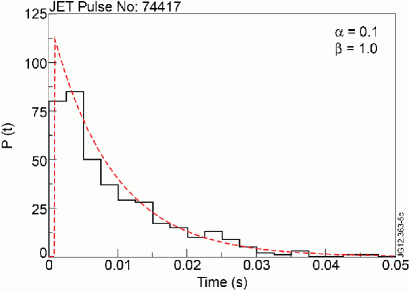
Figure 2: Weibull (blue) and experimental pdfs (black bar chart), for JET shot no. 74417 (type III ELMs).

Figure 6 plots $\alpha$ and $\beta$ for the type I and type III ELM datasets. There is a clear clustering of type III data for $\beta=1$ and $\alpha<0.5$. As noted earlier, $\beta=1$ has special significance because beyond an initial time delay $t_{m}$, it corresponds to a “memoryless” process in which the probability of an ELM is independent of time. The type I data has a wide spread in $\alpha$ and $\beta$, but notably $\beta$ remains of order $2$ or larger. As $\beta$ increases, ELMs will appear increasingly regular. Therefore the type I ELMs studied here are consistent with a process whereby the probability of an ELM increases with time since the previous ELM, possibly due to the build-up of some physical quantity with time. The similarly good agreement between the Gaussian and Weibull fits allows the alternative interpretation that type I ELMs have a specific frequency that is broadened by noise, and that the good fit to type III ELM data is coincidental. This is possible, although our original hypothesis is consistent with present ELM models, and explains the good fit to both the type I and type III data. To avoid disagreement about the classification of ELM types, our dataset excludes ELMs whose type is uncertain. Therefore it is possible that there is a continuum between the classifications that would not be observed in our data set of typical type I and type III ELMs.

As an example we analysed JET plasmas 66105-66109, whose ELM frequency is typical of type III ELMsZohm (1996); Loarte et al. (2003); Kamiya et al. (2007); Rapp , but whose $D_{\alpha}$ signal is visually similar to that of type I ELMs. Based on Fig. 6, they are not type III ELMs.

Figure 3: Maximum-likelihood best fits to Eq. 4: type I ELM database (black diamonds), type III database (blue squares), and some high frequency ELMs (red triangles). Type III data is characterised by $\beta\sim 1$, whereas all other data has $\beta\gtrsim 2$.

Conclusions: We have shown how simple experimentally motivated assumptions require a Weibull pdf for inter-ELM waiting times. The model applies to stationary processes. A search of JET data yielded 64 sufficiently long and steady plasmas to test the model, details of which are in the SM SM . A statistically rigorous ELM detection technique was developed to compare the data sets from experiments many years apart. The method uses a single dimensionless threshold that is set independently of the data, and a single time-period, allowing rapid objective comparisons between different data sets. The dataset was analysed, and a maximum likelihood best fit calculated, finding a good Weibull fit to both type I and type III data. Therefore we explored whether the dimensionless fitting co-efficients $\alpha$ and $\beta$ could be used to classify the data, concluding that they can. The classification has a clear interpretation - type III ELMs are consistent with a memoryless process, but type I ELMs are consistent with the build-up of a quantity with time, leading to instability. In contrast, present ELM classification requires either a subjective judgment, or experimental time to determine how ELM frequency responds to heating Zohm (1996); Loarte et al. (2003); Kamiya et al. (2007).

To summarise, we have shown that a rigorous statistical analysis of ELM waiting times is possible, that it can provide a quantitative classification of ELM types, and physical insight into the processes responsible for them. The methods have numerous potential future applications, especially for the longer plasma pulses planned for ITERITER . These include data mining, use in real-time and for other signals, and a quantitative characterisation of the response of ELM sequences to external parameters.

Acknowledgments: Thanks to B. Alper, G. Maddison, & M. Beurskens for advice on ELM data. This work, supported by the European Communities under the contract of Association between EURATOM and CCFE, was carried out within the framework of the European Fusion Development Agreement. The views and opinions expressed herein do not necessarily reflect those of the European Commission. This work was also part-funded by the RCUK Energy Programme under grant EP/I501045. We acknowledge the UK EPSRC for support.

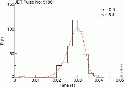
Figure 4: Weibull (blue) and experimental pdfs (black bar chart), for JET pulse no. 57861 (type I ELMs).

Figure 5: Weibull (blue) and experimental pdfs (black bar chart), for JET shot no. 74417 (type III ELMs).

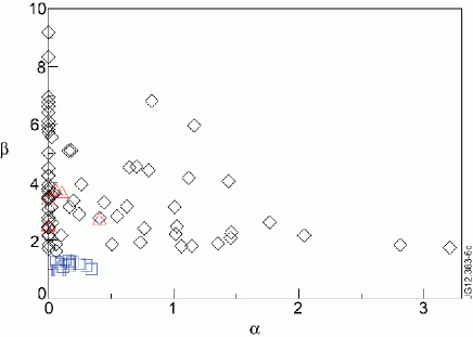
Figure 6: Maximum-likelihood best fits to Eq. 4: type I ELM database (black diamonds), type III database (blue squares), and some high frequency ELMs (red triangles). Type III data is characterised by $\beta\sim 1$, whereas all other data has $\beta\gtrsim 2$.

References

- Keilhacker et al. (1984) M. Keilhacker, Plasma Phys. Control. Fusion 26, 49 (1984)
- Zohm (1996) H. Zohm, Plasma Phys. Control. Fusion 38, 105 (1996)
- Loarte et al. (2003) A. Loarte et al., Plasma Phys. Control. Fusion 45, 1549 (2003)
- Kamiya et al. (2007) K. Kamiya et al., Plasma Phys. Control. Fusion 49, S43 (2007)
- (5) D.C. McDonald et al., Fusion Sci. Technol. 53, 891, (2008)
- (6) J. Rapp et al., Nucl. Fusion 49, 095012, (2009)
- (7) Y. Liang, Fusion Sci. Technol. 59, 586, (2011)
- (8) A.W. Degeling et al., Plasma Phys. Control. Fusion 43, 1671, (2001)
- (9) A.J. Webster, Nucl. Fusion 52, 114023, (2012)
- (10) W. Weibull, Transactions of the American Society of Mechanical Engineers, September issue, 293-297, (1951)
- (11) J. Greenhough, S.C. Chapman, R.O. Dendy, and D.J. Ward, Plasma Phys. Control. Fusion 45, 747 (2003)
- (12) J. Wesson, Tokamaks (Oxford University Press, Oxford, 1997)
- (13) See supplementary material at [] for full details of the datasets studied and the results of their analysis.
- (14) D.S. Sivia, Data Analysis A Bayesian Tutorial (Oxford University Press, Oxford, 2005)
- (15) R. Aymar et al. for THE ITER TEAM, Plasma Phys. Control. Fusion 44, 519 (2002)