Oscillating universe in massive gravity

Abstract

Massive gravity is a modified theory of general relativity. In this paper, we study, using a method in which the scale factor changes as a particle in a “potential”, all possible cosmic evolutions in a ghost-free massive gravity. We find that there exists, in certain circumstances, an oscillating universe or a bouncing one. If the universe starts at the oscillating region, it may undergo a number of oscillations before it quantum mechanically tunnels to the bounce point and then expand forever. But going back to the singularity from the oscillating region is physically not allowed. So, the big bang singularity can be successfully resolved. At the same time, we also find that there exists a stable Einstein static state in some cases. However, the universe can not stay at this stable state past-eternally since it is allowed to quantum mechanically tunnel to a big-bang-to-big-crunch region and end with a big crunch. Thus, a stable Einstein static state universe can not be used to avoid the big bang singularity in massive gravity.

I Introduction

The current accelerated cosmic expansion was discovered firstly from the Type Ia supernovae data Perlmutter1999 ; Riess1998 and further confirmed by many other observations, including the cosmic microwave background radiation Spergel , the large scale structure Eisenstein ; Tegmark , and so on. This discovery broke our common belief that the universe should be undergoing a decelerated expansion. A possible explanation for it among other such as the cosmological constant and the dynamical dark energy is that the theory of general relativity is no longer valid on the cosmological scale and needs to be modified. As a result, many modified gravity theories have been proposed to explain the present accelerated cosmic expansion without the need of the mysterious dark energy. Among them, the Dvali-Gabadadze-Porrati (DGP) model DGP is a very interesting one since it not only admits a self-accelerating solution with only pressureless matter, but also allows the graviton to have a small mass on the cosmological scale.

Actually, about eighty years ago, Fierz and Pauli Fierz first tried to build a theory of massive gravity. However, the linear Fierz-Pauli theory can not recover the linearized Einstein gravity in the limit of zero graviton mass and can not pass the solar system tests due to the van Dam-Veltman-Zakharov (vDVZ) discontinuity van . With the help of Vainshtein mechanism, the introduction of nonlinear interactions can cure this discontinuity Vainshtein ; unfortunately, at the same time, the nonlinear terms also yield the Boulware-Deser (BD) ghost since more than two time derivatives are contained in them Boulware ; Arkani . In order to construct a consistent theory, nonlinear terms should be tuned to remove order by order the negative energy state in the spectrum Boulware . Recently, a ghost-free nonlinear theory of massive gravity was constructed successfully by de Rham, Gabadadze and Tolley (dRGT) Rham . (See, however, Deser for the causality issue of the theory.) It has been found that the dRGT theory can accommodate cosmological solutions with self acceleration Amico and the observational constraint on it has been discussed in Cardone . In addition, the Einstein static state (ES) universe in this massive gravity theory was analyzed in Parisi and it was found that there exist stable ES solutions to avoid the big bang singularity problem. Let us note that the Hawking-Moss instanton in massive gravity has been studied in Ref. Zhangy .

If one writes the Friedmann equation in a form such that the evolution of the cosmic scale factor can be treated as that of a particle in a potential, then it is possible to classify all cosmic evolution types as has been successfully done in the Horava-Lifshitz gravity Maeda2010 and the DGP braneworld scenario Zhang2012 . In this paper, we plan to study all possible cosmic evolutions in the massive gravity with this method. The paper is organized as follows. In Sec. II, we give the Friedmann equation of the massive gravity and define all possible cosmic evolution types. In Sec III, we derive the conditions for the ES solution. We then classify all the cosmic types and give the conditions for them in Sec IV, V and VI, and conclude in Sec VII.

II The Friedmann equation

We consider the theory of massive gravity proposed in Nieuwenhuizen . The action has the form

$$S=\frac{1}{8\pi G}\int\bigg{(}-\frac{1}{2}R+m^{2}\mathcal{L}\bigg{)}\sqrt{-g}d^{4}x+S_{m},$$ (1)

where $G$ is the Newton gravitational constant, $R$ is the Ricci scalar and $\hbar m/c$ is the graviton mass. In the present paper, we let $S_{m}$ describe the ordinary matter plus a possible cosmological constant generated by vacuum energy. $\mathcal{L}$ is the nonlinear higher derivative terms for the massive graviton and it is defined as

$$\mathcal{L}=\frac{1}{2}(S^{2}-S^{A}_{B}S^{B}_{A})+\frac{c_{3}}{3!}\epsilon_{MNPQ}\epsilon^{ABCQ}S^{M}_{A}S^{N}_{B}S^{P}_{C}+\frac{c_{4}}{4!}\epsilon_{MNPQ}\epsilon^{ABCQ}S^{M}_{A}S^{N}_{B}S^{P}_{C}S^{Q}_{D},$$ (2)

where $S=S^{A}_{A}$, $c_{3}$ and $c_{4}$ are two constants, $\epsilon_{MNPQ}$ is the Levi-Civita tensor density and

$$S^{A}_{B}=\delta^{A}_{B}-\gamma^{A}_{B}\;.$$ (3)

Here $\gamma^{A}_{B}$ is defined by

$$\gamma^{A}_{B}\gamma_{A}^{C}=g^{AC}f_{AB}$$ (4)

with $f_{AB}$ being a symmetric tensor field.

The Robertson-Walker (RW) metric for a spatially homogeneous and isotropic universe can be written as

$$ds^{2}=dt^{2}-a^{2}(t)\bigg{(}\frac{dr^{2}}{1-kr^{2}}+r^{2}d^{2}\Omega\bigg{)}\;,$$ (5)

where $a$ is the cosmic scale factor, $t$ is the cosmic time and $k=0,\pm 1$ is the constant curvature of three dimensional space. In massive gravity, Chamseddine and Volkov show that there exist cosmological solutions where the effect of the graviton mass is equivalent to introducing to the Friedmann equation a matter source that can consist of several different matter types besides a cosmological constant term Chamseddine2011

$$H^{2}+\frac{k}{a^{2}}=\frac{m^{2}}{3}\bigg{(}4c_{3}+c_{4}-6+3C\frac{3-3c_{3}-c_{4}}{a}+3C^{2}\frac{c_{4}+2c_{3}-1}{a^{2}}$$

$$-C^{3}\frac{c_{3}+c_{4}}{a^{3}}\bigg{)}+\frac{8\pi G\rho}{3},$$ (6)

where $H\equiv\frac{\dot{a}}{a}$ is the Hubble parameter, $C$ is an integration constant and $\rho$ is the energy density of ordinary matter plus vacuum energy. Here, besides the cosmological term, three additional terms in the Friedmann equation which decay as $1/a$, $1/a^{2}$ and $1/a^{3}$ can be viewed as quintessence, gas of cosmic strings, and non-relativistic cold matter respectively. Thus, the massive gravity can explain the present accelerated cosmic expansion. At the same time, it may also play an important role in the very early universe (when $a$ is very small). In the present paper, we plan to study the all the possible cosmic evolutions in massive gravity and whether the big bang singularity can be avoided. Note that, by employing the familiar canonical quantization procedure in massive gravity for an open cosmic background, Vakili and Khosravi found that the big bang singularity can be avoided through a bounce Vakili . For simplicity, we only consider a spatially flat universe $k=0$ and a positive constant $C$. In addition, since we are interested in the very early universe, the vacuum energy is assumed to be the only cosmic energy component and then $\rho$ is a positive constant. Defining $\Lambda\equiv\frac{8\pi G\rho}{3m^{2}}$ and rescaling $a/C\rightarrow a$, we can re-express the Friedmann equation (Eq. (II)) as

$$H^{2}=\frac{m^{2}}{3}\bigg{(}4c_{3}+c_{4}-6+3\Lambda+3\frac{3-3c_{3}-c_{4}}{a}+3\frac{c_{4}+2c_{3}-1}{a^{2}}-\frac{c_{3}+c_{4}}{a^{3}}\bigg{)}\;.$$ (7)

Let us now write the above Friedmann equation into the following form

$$\dot{a}^{2}+V(a)=0,$$ (8)

where

$$V(a)=-m^{2}\bigg{[}\frac{1}{3}(4c_{3}+c_{4}-6+3\Lambda)a^{2}+(3-3c_{3}-c_{4})a+$$

$$(c_{4}+2c_{3}-1)-\frac{1}{3}(c_{3}+c_{4})\frac{1}{a}\bigg{]}.$$ (9)

Thus the evolution of the scale factor $a$ can be considered as that of a particle moving in a “potential” $V$. Obviously, this “potential” must satisfy the condition $V(a)\leq 0$, and this gives the possible ranges of $a$ as the universe evolves. Since the values of $\Lambda$, $c_{3}$ and $c_{4}$ determine the potential $V(a)$, we can use them to classify all possible cosmic types.

All types of the universe in the theory of massive gravity are:

(1) [Bounce]: If $V(a)\leq 0$ for $a\in[a_{T},\infty)$ and the equality holds at $a=a_{T}$, the spacetime initially contracts from an infinite scale, and it eventually turns around at a finite scale $a_{T}$, and then expands forever.

(2) [Oscillation]: $V(a)\leq 0$ for $a\in[a_{min},a_{max}]$ and the equality occurs at $a=a_{min}$ and $a=a_{max}$. Thus, the spacetime oscillates between two finite scales.

(3) [$BB\Rightarrow BC$]: $V(a)\leq 0$ for $a\in(0,a_{T}]$ and the equality holds at $a=a_{T}$. The universe starts from a big bang (BB) and expands. Eventually it turns around at $a=a_{T}$ and contracts to a big crunch (BC). $a_{T}$ is the scale factor where the universe turns around from expansion to contraction.

(4) [$BB\Rightarrow\infty$ or $\infty\Rightarrow BC$]: $V(a)<0$ for any positive values of $a$. The spacetime starts from a big bang and expands forever, or the spacetime always contracts to a big crunch.

III Einstein static state solution

Since we assume that the universe is dominated only by vacuum energy, $\rho$ must be a positive constant, and thus $\Lambda=\frac{8\pi G\rho}{3m^{2}}>0$. The potential (Eq. (II)) can be re-expressed as

$$V(a)=-\frac{m^{2}}{3a}(4c_{3}+c_{4}-6+3\Lambda)\bigg{(}a^{3}+\frac{3(3-3c_{3}-c_{4})}{(4c_{3}+c_{4}-6+3\Lambda)}a^{2}+$$

$$\frac{3(c_{4}+2c_{3}-1)}{(4c_{3}+c_{4}-6+3\Lambda)}a-\frac{(c_{3}+c_{4})}{(4c_{3}+c_{4}-6+3\Lambda)}\bigg{)},$$ (10)

which means that $V(a)=0$ yields a cubic equation of $a$. An ES universe appears if there is a solution $a=a_{s}>0$ which satisfies $V(a_{s})=0$ and $V^{\prime}(a_{s})=0$. At $a_{s}$, both the speed of the cosmic expansion and acceleration are equal to zero and thus the universe can stay at this point in a long time if it is stable. Differentiating $V(a)$ with respect to $a$, we have

$$V^{\prime}(a)=-\frac{m^{2}}{3a^{2}}\bigg{(}2(4c_{3}+c_{4}-6+3\Lambda)a^{3}+3(3-3c_{3}-c_{4})a^{2}+(c_{3}+c_{4})\bigg{)}\;.$$ (11)

Combining $V(a)=0$ and $V^{\prime}(a)=0$, we find that an ES solution requires a relation between $\Lambda$ and other two model parameters $c_{3}$, $c_{4}$ to hold

$$\Lambda=\Lambda^{\pm}=\frac{\pm 2[1+(c_{3}-1)c_{3}+c_{4}]^{\frac{3}{2}}-(c_{3}-1)[2+c_{3}(2c_{3}-1)+3c_{4}]}{3(c_{3}+c_{4})^{2}}\;.$$ (12)

They give two boundaries for obtaining an oscillating universe. Substituting Eq. (12) into the equation $V(a)=0$ or $V^{\prime}(a)=0$, one can find that the following static state solutions

$$a_{s}=a_{s}^{\pm}=\frac{2c_{3}+c_{4}-1\pm\sqrt{1+(-1+c_{3})c_{3}+c_{4}}}{3c_{3}+c_{4}-3}\;,$$ (13)

which is a double root of the equation $V(a)=0$ under the condition $V^{\prime}(a)=0$, and the third root is

$$a_{T}=a_{T}^{\pm}=\frac{c_{3}+c_{4}}{-1+2c_{3}+c_{4}\pm 2\sqrt{1+(-1+c_{3})c_{3}+c_{4}}}\;.$$ (14)

If $a_{T}$ is positive, it corresponds to the radius where the universe turns around or bounces.

Since the sign of $4c_{3}+c_{4}-6+3\Lambda$, which is the coefficient of the $a^{3}$ term in the potential, plays a crucial role in determining the shape of the potential $V(a)$, we will divide our following discussions into three different cases: $4c_{3}+c_{4}-6+3\Lambda>0$, $4c_{3}+c_{4}-6+3\Lambda<0$ and $4c_{3}+c_{4}-6+3\Lambda=0$.

IV the case of $4c_{3}+c_{4}-6+3\Lambda>0$

The condition $4c_{3}+c_{4}-6+3\Lambda>0$ gives rise to a constraint on $\Lambda$, i.e., $\Lambda>-\frac{1}{3}(4c_{3}+c_{4}-6)$. We find that, when $\Lambda$ takes different values, the number of real roots for $V(a)=0$ is different. For example, $\Lambda=\Lambda^{+}$ allows the existence of three roots, where $\Lambda^{+}$ is defined in Eq. (12), but two of them are double, which corresponds to an unstable ES solution. In order to illustrate our results more clearly, we further divide our discussion into three subcases, i.e., $\Lambda^{-}\leq\Lambda\leq\Lambda^{+}$, $\Lambda<\Lambda^{-}$ and $\Lambda>\Lambda^{+}$, respectively.

IV.1 $\Lambda^{-}\leq\Lambda\leq\Lambda^{+}$

In this case, $V(a)=0$ yields a cubic equation of $a$, which has three real roots. Assuming $a_{1}$, $a_{2}$ and $a_{3}$ are three real roots of this cubic equation, respectively, Eq. (III) can be expressed as

$$V(a)=-\frac{2m^{2}}{3a}(4c_{3}+c_{4}-6+3\Lambda)(a-a_{1})(a-a_{2})(a-a_{3}).$$ (15)

Since $\Lambda>0$ and $(4c_{3}+c_{4}-6+3\Lambda)>0$, the existence of three real roots requires that $\Lambda$ must satisfy the condition

$$Max\;\bigg{\{}0,-\frac{1}{3}(4c_{3}+c_{4}-6)\bigg{\}}<\Lambda\leq\Lambda^{+}\;,$$ (16)

if $\Lambda^{-}\leq Max\;\{0,-\frac{1}{3}(4c_{3}+c_{4}-6)\}$, or

$$\Lambda^{-}\leq\Lambda\leq\Lambda^{+}\;,$$ (17)

if $\Lambda^{-}>Max\;\{0,-\frac{1}{3}(4c_{3}+c_{4}-6)\}$. Since the cosmic scale factor must be larger than zero ($a>0$), next, we will only consider the cases of positive roots.

IV.1.1 three positive roots

Using $a_{min}$, $a_{max}$ and $a_{T}$ to represent three positive roots of $V(a)=0$ and assuming $0<a_{min}\leq a_{max}\leq a_{T}$, we have

$$V(a) = -\frac{2m^{2}}{3a}(4c_{3}+c_{4}-6+3\Lambda)(a-a_{min})(a-a_{max})(a-a_{T})$$ (18)

$$= -\frac{2m^{2}}{3a}(4c_{3}+c_{4}-6+3\Lambda)\bigg{(}a^{3}-(a_{min}+a_{max}+a_{T})a^{2}+$$

$$(a_{min}a_{max}+a_{T}a_{min}+a_{max}a_{T})a-a_{min}a_{max}a_{T}\bigg{)}.$$

Three positive roots mean that $a_{min}+a_{max}+a_{T}>0$, $a_{min}a_{max}+a_{T}a_{min}+a_{max}a_{T}>0$, and $a_{min}a_{max}a_{T}>0$. Using these conditions and $4c_{3}+c_{4}-6+3\Lambda>0$, and comparing Eq. (III) and Eq. (18), one can obtain three inequalities:

$$3-3c_{3}-c_{4}<0\;,\;\;c_{4}+2c_{3}-1>0\;,\;\;\;c_{3}+c_{4}>0\;.$$ (19)

When the above inequalities are satisfied, $\Lambda^{-}$ is negative or imaginary. Thus, $\Lambda$ is required to only satisfy

$$Max\;\bigg{\{}-\frac{1}{3}(4c_{3}+c_{4}-6),0\bigg{\}}<\Lambda\leq\Lambda^{+}.$$ (20)

First, we consider the case of three different positive roots, which requires $Max\;\{-\frac{1}{3}(4c_{3}+c_{4}-6),0\}<\Lambda<\Lambda^{+}$, and the $\Lambda=\Lambda^{+}$ case will be dealt with separately. From this condition and Eq. (19), we find that three different positive roots demand

$$c_{3}\leq\frac{3}{2}\;,\;\;\;c_{3}+c_{4}>3-2c_{3}\;,$$

$$or c_{3}>\frac{3}{2}\;,\;\;\;c_{3}+c_{4}>0\;.$$ (21)

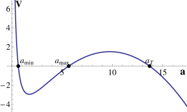
Figure 1: Potential ${V}(a)$ under the conditions given in Eq. (IV.1.1) and $Max\;\{-\frac{1}{3}(4c_{3}+c_{4}-6),0\}<\Lambda<\Lambda^{+}$. An oscillating universe or a bouncing one is obtained. The constants are chosen as $m=1$, $c_{3}=-5$, $c_{4}=20$, and $\Lambda=2.1$. The radii are $a_{min}=0.64503$, $a_{max\;}=5.66024$ and $a_{T}=13.69470$. The period of an oscillation is $T=5.52532$.

As shown in Fig. (1), $V(a)\leq 0$ in $a\in[a_{min},a_{max}]$ with the equality holding at $a=a_{min}$ and $a=a_{max\;}$, and $a\in[a_{T},\infty)$ with $V(a_{T})=0$. This means that the universe oscillates between $a_{min}$ and $a_{max\;}$ or bounces at $a_{T}$. Thus, if the universe is in the region $[a_{min},a_{max\;}]$ initially, it may undergo oscillation. After a number of oscillations, it may evolve to the bounce point $a_{T}$ through quantum tunneling but tunneling to the big bang singularity is not allowed. While, if the universe contracts initially from an infinite scale, it will turn around at $a_{T}$ and then expand forever. So, the big bang singularity can be avoided in this case and a successful emergent universe is achieved.

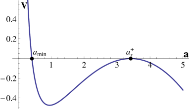
Figure 2: Potential $V(a)$ with model parameters satisfying Eq. (IV.1.1) and $\Lambda=\Lambda^{+}$. There is an unstable static state universe and a bouncing one. The constants are chosen as $m=1$, $c_{3}=1$, $c_{4}=1$, and $\Lambda=0.47141$. We obtain $a_{min}=0.41421$ and $a_{s}^{+}=3.41421$.

When $\Lambda=\Lambda^{+}$ in Eq. (20), $a_{T}$ and $a_{max\;}$ coincide with each other, which corresponds to a double solution. We represent this double solution by $a_{s}^{+}$ which is given in Eq. (13), and find that $c_{3}$ and $c_{4}$ are required to satisfy Eq. (IV.1.1), too. In Fig. (2), we plot the evolutionary curve of $V(a)$ with $\Lambda=\Lambda^{+}$. It is easy to see that $a_{s}^{+}$ is an unstable ES solution. Therefore, the universe can oscillate between $a_{min}$ and $a_{s}^{+}$, and it can also evolve directly from $a_{min}$ to $\infty$ or evolve to $\infty$ after some oscillations without the help of quantum tunneling. If the universe contracts initially from an infinite scale, it can turn around at $a_{s}^{+}$, or pass $a_{s}^{+}$ and bounce at $a_{min}$, then directly expand forever or do so after a number of oscillations between $a_{min}$ and $a_{s}^{+}$.

In Fig. (3), we plot the phase diagram of spacetimes in $(c_{3},c_{4})$ plane. Three positive roots restrict $c_{3}$ and $c_{4}$ to Region 1.

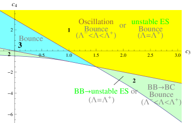
Figure 3: Phase diagram of spacetimes in $(c_{3},c_{4})$ plane when $\Lambda^{-}\leq\Lambda\leq\Lambda^{+}$. An oscillating universe is found in Region 1 and a bouncing one is obtained in Regions 1, 2, and 3.

IV.1.2 two positive roots

In this case, two of three real roots are positive and one of them is negative. We assume $a_{1}<0<a_{2}\leq a_{3}$, and set $a_{2}=a_{T1}$ and $a_{3}=a_{T2}$ since $a_{2}$ and $a_{3}$ are two bouncing points. Then, we have

$$a_{1}a_{T1}a_{T2}=\frac{(c_{3}+c_{4})}{(4c_{3}+c_{4}-6+3\Lambda)}<0\;.$$ (22)

Of course, this condition corresponds to two different cases: three negative roots or two positive roots and one negative one. In order to distinguish these two cases, we further consider the signs of $a_{1}+a_{T1}+a_{T2}$ and $a_{1}a_{T1}+a_{T1}a_{T2}+a_{1}a_{T2}$. When $a_{1}+a_{T1}+a_{T2}\geq 0$, there is at least one positive root, which must correspond to the case of two positive roots and one negative one. When $a_{1}+a_{T1}+a_{T2}<0$, three negative roots lead to $a_{1}a_{T1}+a_{T1}a_{T2}+a_{1}a_{T2}>0$, while, $a_{1}<0<a_{T1}\leq a_{T2}$ implies that $a_{1}a_{T1}+a_{T1}a_{T2}+a_{1}a_{T2}=a_{1}(a_{T1}+a_{T2})+a_{T1}a_{T2}<-(a_{T1}+a_{T2})^{2}+a_{T1}a_{T2}=-(a_{T1}+\frac{1}{2}a_{T2})^{2}-\frac{3}{4}a_{T2}^{2}<0$. Thus, the conditions for two positive roots and a negative one are:

$$c_{3}+c_{4}<0\;,\;\;-(3-3c_{3}-c_{4})\geq 0\;,$$

$$or c_{3}+c_{4}<0\;,\;\;-(3-3c_{3}-c_{4})<0\;,\;\;c_{4}+2c_{3}-1<0\;.$$ (23)

Same as in the previous subsection, $\Lambda^{-}$ is negative or imaginary when the above inequalities are satisfied, so, $\Lambda$ is required to only obey

$$Max\;\bigg{\{}-\frac{1}{3}(4c_{3}+c_{4}-6),0\bigg{\}}<\Lambda\leq\Lambda^{+}\;.$$ (24)

We first consider $Max\;\{-\frac{1}{3}(4c_{3}+c_{4}-6),0\}<\Lambda<\Lambda^{+}$, which corresponds to the case of two different positive roots. Combing this condition with Eq. (IV.1.2), we find that there exist two different positive roots and one negative one when

$$c_{3}<1\;,\;\;3-c_{3}-2\sqrt{3-3c_{3}+c_{3}^{2}}<c_{3}+c_{4}<0\;,$$

$$\frac{3}{2}<c_{3}\leq 2\;,\;\;3-2c_{3}<c_{3}+c_{4}<0\;,$$

$$or c_{3}>2\;,\;\;3-c_{3}-2\sqrt{3-3c_{3}+c_{3}^{2}}<c_{3}+c_{4}<0\;.$$ (25)

Above conditions correspond to Region 2 in Fig. (3) .

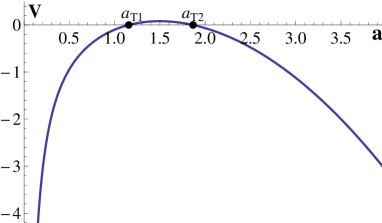
Figure 4: The potential ${V}(a)$ for a $BB\Rightarrow BC$ universe or a bouncing one with $Max\;\{-\frac{1}{3}(4c_{3}+c_{4}-6),0\}<\Lambda<\Lambda^{+}$ and model parameters in Region 2 of Fig. (3). The constants are chosen as $m=1$, $c_{3}=3$, $c_{4}=-5$, and $\Lambda=0.1$. The radii are $a_{T1}=1.15556$ and $a_{T2}=1.86572$.

Fig. (4) shows the evolution of the potential ${V}(a)$ with the model parameters in Region 2 of Fig. (3). From this figure, we find that a $BB\Rightarrow BC$ universe or a bouncing one is obtained since $V\leq 0$ in $a\in(0,a_{T1}]$ and $[a_{T2},\infty)$ with $V=0$ occurring at $a=a_{T1}$ and $a=a_{T2}$. Thus, if the universe initiates from a big bang, it can expand to $a_{T1}$. It then turns over at $a_{T1}$ and ends with a big crunch. In addition, it is also possible that the universe quantum tunnels to $a_{T2}$ directly from $a_{T1}$ and then expands forever. If the universe contracts initially from infinity, a bounce will occur at $a_{T2}$.

When $\Lambda=\Lambda^{+}$, $a_{T1}$ and $a_{T2}$ coincide with each other and a double root $a_{s}^{+}$ given in Eq. (13) is obtained. $c_{3}$ and $c_{4}$ are required to satisfy Eq. (IV.1.2), too. As shown in Fig (5), the ES solution $a_{s}^{+}$ is unstable. So, if the universe initiates from big bang, it will expand to an unstable ES universe and then turn over or expand forever. If the universe contracts from infinity initially, it can bounce at $a_{s}^{+}$ or end with a big crunch.

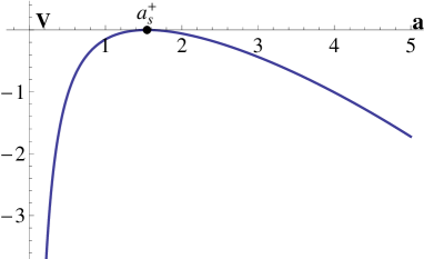
Figure 5: Potential $V(a)$ with $c_{3}$ and $c_{4}$ in Region 2 of Fig. (3), and $\Lambda=\Lambda^{+}$. A big bang universe and an unstable ES solution are obtained. The constants are chosen as $m=1$, $c_{3}=3$, $c_{4}=-6.3$ and $\Lambda=0.15217$. We find $a_{s}^{+}=1.54447$.

IV.1.3 one positive root

For this case, only one of three real roots is positive and two of them are negative. Assuming that $a_{1},a_{2}<0$ and $a_{3}=a_{T}>0$, one has

$$a_{1}a_{2}a_{T}=\frac{(c_{3}+c_{4})}{(4c_{3}+c_{4}-6+3\Lambda)}>0.$$ (26)

Since this condition can correspond to either three positive roots or one positive root and two negative ones, we have to consider other conditions coming from $a_{1}+a_{2}+a_{T}$ and $a_{1}a_{2}+a_{2}a_{T}+a_{1}a_{T}$. If $a_{1}+a_{2}+a_{T}\leq 0$, there is at least one negative root regardless of the value of $a_{1}a_{2}+a_{2}a_{T}+a_{1}a_{T}$. Thus,

$$c_{3}+c_{4}>0\;,\;\;-(3-3c_{3}-c_{4})\leq 0\;,$$ (27)

are sufficient for having one positive root and two negative ones. If $a_{1}+a_{2}+a_{T}>0$, the condition from $a_{1}a_{2}+a_{2}a_{T}+a_{1}a_{T}$ should be added. When $a_{1},a_{2},a_{T}>0$ (three positive roots), $a_{1}a_{2}+a_{2}a_{T}+a_{1}a_{T}>0$. However, if $a_{1}<a_{2}<0<a_{T}$, then $a_{1}a_{2}+a_{2}a_{T}+a_{1}a_{T}=a_{T}(a_{1}+a_{2})+a_{1}a_{2}<-(a_{1}+a_{2})^{2}+a_{1}a_{2}=-(a_{1}-\frac{1}{2}a_{2})^{2}-\frac{3}{4}a_{2}^{2}<0$. So,

$$c_{3}+c_{4}>0\;,\;\;-(3-3c_{3}-c_{4})>0\;,\;\;c_{4}+2c_{3}-1<0\;,$$ (28)

give the conditions in obtaining one positive root and two negative ones. Since $\Lambda^{-}<0$ if Eq. (27) or Eq. (28) is satisfied, we only consider

$$Max\;\bigg{\{}-\frac{1}{3}(4c_{3}+c_{4}-6),0\bigg{\}}<\Lambda<\Lambda^{+}\;.$$ (29)

Here, $\Lambda=\Lambda^{+}$ is discarded because in this case there is no double solution. That is, there is no unstable ES solution. Combining Eqs. (27) and (29), or Eqs. (28) and (29), one can find the conditions for the existence of one positive root and two negative ones

$$c_{3}<\frac{3}{2}\;\;,\;0<c_{3}+c_{4}<3-2c_{3}\;,$$ (30)

which is shown as Region 3 in Fig. (3). Fig. (6) shows the evolutionary curve of the potential ${V}(a)$ with model parameters in Region 3 in Fig. (3). Apparently, a bouncing universe is obtained.

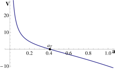
Figure 6: Potential ${V}(a)$ with $Max\;\{-\frac{1}{3}(4c_{3}+c_{4}-6),0\}<\Lambda<\Lambda^{+}$ and model parameters in Region 3 of Fig. (3). A bouncing universe is obtained. The constants are chosen as $m=1$, $c_{3}=-3$, $c_{4}=6$, and $\Lambda=10$. The turning radius at a bounce is $a_{T}=0.408248$.

IV.1.4 no positive root

Three real roots are all negative. Fig. (7) shows the evolutionary curve of $V(a)$ in this case. One can see that the potential is always negative and the cosmic evolution type is $BB\Rightarrow\infty$ or $\infty\Rightarrow BC$.

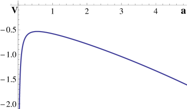
Figure 7: Potential ${V}(a)$ for the case of no positive root. A $BB\Rightarrow\infty$ or $\infty\Rightarrow BC$ cosmic type is obtained. The constants are chosen as $m=1$, $c_{3}=1.5$, $c_{4}=-1.7$, and $\Lambda=0.58$.

IV.2 $\Lambda>\Lambda^{+}$

In this case, $\Lambda$ must satisfy

$$\Lambda>Max\;\bigg{\{}\Lambda^{+},-\frac{1}{3}(4c_{3}+c_{4}-6),0\bigg{\}}\;.$$ (31)

Under this condition, there is only one real root, which can be positive or negative, and other two roots are a conjugate imaginary pair. In Fig. (8), we show all possible cosmic types in $(c_{3},c_{4})$ plane.

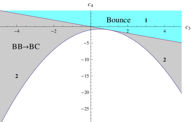
Figure 8: Phase diagram of spacetimes in $(c_{3},c_{4})$ plane with $\Lambda>\Lambda^{+}$. A bouncing universe is found in Region 1, while, a $BB\Rightarrow BC$ one is obtained in Region 2.

IV.2.1 one positive root

Assuming that $a_{1}$ and $a_{2}$ are two conjugate imaginary roots and $a_{3}$ is the only positive one, and setting $a_{3}=a_{T}$, one has

$$a_{1}a_{2}a_{T}=\frac{(c_{3}+c_{4})}{(4c_{3}+c_{4}-6+3\Lambda)}>0.$$ (32)

Combining this inequality with Eq. (31), we get the condition for one positive root and two conjugate imaginary ones

$$c_{3}+c_{4}>0,$$ (33)

which corresponds to Region $1$ of Fig. (8). Fig. (9) shows the evolution of the potential ${V}(a)$ with model parameters in Region 1 of Fig. (8). We find that a bouncing universe is obtained.

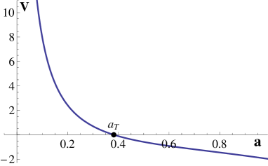
Figure 9: Potential $V(a)$ for a bouncing universe with model parameters in Region 1 of Fig. (8) and $\Lambda>\Lambda^{+}$. The constants are chosen as $m=1$, $c_{3}=1.5$, $c_{4}=2$, and $\Lambda=2$. The turning radius at a bounce is $a_{T}=0.3823023$.

IV.2.2 no positive root

In this case, the only real root is negative, which gives

$$a_{1}a_{2}a_{3}=\frac{(c_{3}+c_{4})}{(4c_{3}+c_{4}-6+3\Lambda)}<0\;.$$ (34)

From the above inequality and the condition given in Eq. (31), one has

$$c_{3}\neq 1\;,\;\;-(c_{3}-1)^{2}<c_{3}+c_{4}<0\;,$$ (35)

which correspond to Region 2 in Fig. (8). Fig. (10) shows that the potential is always negative and the cosmic type is $BB\Rightarrow\infty$ or $\infty\Rightarrow BC$.

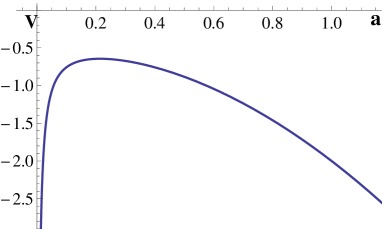
Figure 10: Potential $V(a)$ for a $BB\Rightarrow\infty$ or $\infty\Rightarrow BC$ universe with $\Lambda>\Lambda^{+}$ and model parameters in Region 2 of Fig. (8). The constants are chosen as $m=1$, $c_{3}=1.5$, $c_{4}=-1.6$, and $\Lambda=2$.

IV.3 $\Lambda<\Lambda^{-}$

It is easy to see that here $\Lambda$ must satisfy

$$Max\;\bigg{\{}0,-\frac{1}{3}(4c_{3}+c_{4}-6)\bigg{\}}<\Lambda<\Lambda^{-}.$$ (36)

One can show that there is only one real root and it is negative. Other two roots are a conjugate imaginary pair. Model parameters $c_{3}$ and $c_{4}$ are restricted in the region:

$$1<c_{3}<2\;,\;\;-(c_{3}-1)^{2}\leq c_{3}+c_{4}<3-c_{3}-2\sqrt{3-3c_{3}+c_{3}^{2}}\;.$$ (37)

The evolution of the potential is shown in Fig. (11). One can see that the cosmic type is $BB\Rightarrow\infty$ or $\infty\Rightarrow BC$.

In Tab. (1), we sum up the results obtained in this section.

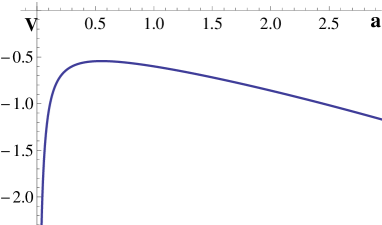
Figure 11: Potential $V(a)$ under the condition $\{0,-\frac{1}{3}(4c_{3}+c_{4}-6)\}<\Lambda<\Lambda^{-}$ and model parameters satisfying Eq. (37). A $BB\Rightarrow\infty$ or $\infty\Rightarrow BC$ universe is obtained. The constants are chosen as $m=1$, $c_{3}=1.5$, $c_{4}=-1.74$, and $\Lambda=0.6$.

Table 1: Summary of the cosmic type in the $4c_{3}+c_{4}-6+3\Lambda>0$ case

$\Lambda$	$c_{3},\;c_{4}$	Cosmic Type
	$c_{3}\leq\frac{3}{2},\;c_{3}+c_{4}>3-2c_{3}$	Oscillation
	$or~{}c_{3}>\frac{3}{2},\;c_{3}+c_{4}>0$	or Bounce
$Max\;\{-\frac{1}{3}(4c_{3}+c_{4}+6),0\}$	$c_{3}<1,\;\;3-c_{3}-2\sqrt{3-3c_{3}+c_{3}^{2}}<c_{3}+c_{4}<0$	$BB\Rightarrow BC$
$<\Lambda<\Lambda^{+}$	$\frac{3}{2}<c_{3}\leq 2,\;3-2c_{3}<c_{3}+c_{4}<0$	or Bounce
	$or~{}c_{3}>2,\;3-c_{3}-2\sqrt{3-3c_{3}+c_{3}^{2}}<c_{3}+c_{4}<0$
	$c_{3}<\frac{3}{2},\;0<c_{3}+c_{4}<3-2c_{3}$	Bounce
	$c_{3}\leq\frac{3}{2},\;c_{3}+c_{4}>3-2c_{3}$	Bounce
	$or~{}c_{3}>\frac{3}{2},\;c_{3}+c_{4}>0$	Unstable ES
$\Lambda=\Lambda^{+}$	$c_{3}<1,\;\;3-c_{3}-2\sqrt{3-3c_{3}+c_{3}^{2}}<c_{3}+c_{4}<0$	$BB\Rightarrow\infty$
	$\frac{3}{2}<c_{3}\leq 2,\;3-2c_{3}<c_{3}+c_{4}<0$	$BB\Rightarrow BC$
	$or~{}c_{3}>2,\;3-c_{3}-2\sqrt{3-3c_{3}+c_{3}^{2}}<c_{3}+c_{4}<0$	$\infty\Rightarrow BC$
		or Bounce
		Unstable ES
$\Lambda>$	$c_{3}+c_{4}>0$	Bounce
$Max\big{\{}\Lambda^{+},-\frac{1}{3}(4c_{3}+c_{4}-6),0\big{\}}$	$c_{3}\neq 1,\;\;-(c_{3}-1)^{2}<c_{3}+c_{4}<0$	$BB\Rightarrow\infty$
		or $\infty\Rightarrow BC$
$Max\;\big{\{}0,-\frac{1}{3}(4c_{3}+c_{4}-6)\big{\}}$	$1<c_{3}<2,$	$BB\Rightarrow\infty$
$<\Lambda<\Lambda^{-}$	$-(c_{3}-1)^{2}\leq c_{3}+c_{4}<3-c_{3}-2\sqrt{3-3c_{3}+c_{3}^{2}}$	or $\infty\Rightarrow BC$

V The case of $3\Lambda+4c_{3}+c_{4}-6<0$

As in the preceding section, we divide our discussion into three different subcases: $\Lambda^{-}\leq\Lambda\leq\Lambda^{+}$, $\Lambda<\Lambda^{-}$ and $\Lambda>\Lambda^{+}$, respectively.

V.1 $\Lambda^{-}\leq\Lambda\leq\Lambda^{+}$

In this case, the equation $V(a)=0$ has three real roots and we assume them to be $a_{1}$, $a_{2}$ and $a_{3}$, respectively. Since a positive $\Lambda$ is considered, $\Lambda$ must satisfy

$$0<\Lambda<-\frac{1}{3}(4c_{3}+c_{4}-6)$$ (38)

and

$$\Lambda^{-}\leq\Lambda\leq\Lambda^{+}\;.$$ (39)

V.1.1 three positive roots

Letting $a_{1}=a_{T}$, $a_{2}=a_{min}$, and $a_{3}=a_{max}$, and assuming $0\leq a_{T}\leq a_{min}\leq a_{max}$, we can re-express Eq. (III) as

$$V(a)=-\frac{2m^{2}}{3a}(4c_{3}+c_{4}-6+3\Lambda)(a-a_{T})(a-a_{min})(a-a_{max\;})$$

$$=-\frac{2m^{2}}{3a}(4c_{3}+c_{4}-6+3\Lambda)\bigg{(}a^{3}-(a_{T}+a_{min}+a_{max\;})a^{2}+$$

$$(a_{T}a_{min}+a_{min}a_{max}+a_{T}a_{max})a-a_{T}a_{min}a_{max\;}\bigg{)}\;.$$ (40)

Three positive roots imply that $a_{T}+a_{min}+a_{max\;}>0$, $a_{T}a_{min}+a_{min}a_{max}+a_{T}a_{max}>0$ and $a_{T}a_{min}a_{max\;}>0$. Comparing Eq. (III) and Eq. (V.1.1), one has

$$3-3c_{3}-c_{4}>0\;,\;\;c_{4}+2c_{3}-1<0\;,\;\;c_{3}+c_{4}<0.$$ (41)

We first study the case of $\Lambda\neq\Lambda^{+}$ and $\Lambda\neq\Lambda^{-}$, which corresponds to three different positive roots. Combining Eqs. (38, 39) and Eq. (41), we obtain that three different positive roots require

$$c_{3}<1\;,\;\;-\frac{3}{4}(c_{3}-1)^{2}<c_{3}+c_{4}<0\;,$$

$$2<c_{3}\leq 3\;,\;\;-(c_{3}-1)^{2}<c_{3}+c_{4}<3-2c_{3}\;,$$

$$or c_{3}>3\;,\;\;-(c_{3}-1)^{2}<c_{3}+c_{4}<6-3c_{3}\;,$$ (42)

which give Region 1 in Fig. (12). The cosmic type is $BB\Rightarrow BC$ or oscillation, as can be seen from Fig. (13). Thus, if the universe starts from a big bang, it can expand to $a_{T}$, then turn over at $a_{T}$ and end with a big crunch. If the universe is in the region $a\in[a_{min},a_{max\;}]$ initially, it may undergo an oscillation. After some oscillations, it may quantum mechanically tunnel to $a_{T}$ and end with a big crunch singularity. Therefore, the classical singularity still exists.

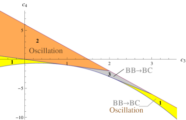
Figure 12: Phase diagram of spacetimes in $(c_{3},c_{4})$ plane under the condition of $\Lambda^{-}<\Lambda<\Lambda^{+}$. An oscillating universe is found in Regions 1 and 2, and a $BB\Rightarrow BC$ universe is obtained in Regions 1 and 3.

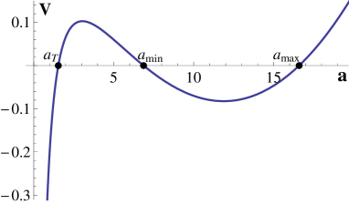
Figure 13: Potential ${V}(a)$ for a $BB\Rightarrow BC$ universe or an oscillating one with model parameters in Region 1 of Fig. (12). The constants are chosen as $m=1$, $c_{3}=2.5$, $c_{4}=-4.6$, and $\Lambda=0.196$. The radii are $a_{T}=1.53548$, $a_{min}=6.86654$ and $a_{max\;}=16.598$. The period of an oscillation is $T=107.478$.

When $\Lambda=\Lambda^{+}$ and $\Lambda$ satisfies $0<\Lambda<-\frac{1}{3}(4c_{3}+c_{4}-6)$, $a_{T}$ and $a_{min}$ coincide with each other and forms a double positive root $a_{s}^{+}$ defined in Eq. (13). Fig. (14) shows that $a_{s}^{+}$ is an unstable ES solution. The cosmic type is $BB\Rightarrow BC$. But, the universe can turn over at $a_{s}^{+}$, or $a_{max}$. From Eq. (V.1.1) and $0<\Lambda=\Lambda^{+}<-\frac{1}{3}(4c_{3}+c_{4}-6)$, we obtain the conditions on $c_{3}$ and $c_{4}$ for an unstable Einstein static state solution:

$$c_{3}<1\;,\;\;-\frac{3}{4}(c_{3}-1)^{2}<c_{3}+c_{4}<3-c_{3}-2\sqrt{3-3c_{3}+c_{3}^{2}}\;,$$

$$or c_{3}>2\;,\;\;-(c_{3}-1)^{2}\leq c_{3}+c_{4}<3-c_{3}-2\sqrt{3-3c_{3}+c_{3}^{2}}\;.$$ (43)

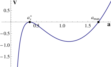
Figure 14: The potential $V(a)$ under the condition $\Lambda=\Lambda^{+}$. An unstable ES solution is obtained. The constants are chosen as $m=1$, $c_{3}=-1$, $c_{4}=-1$, and $\Lambda=0.804738$. The radii are $a_{s}^{+}=0.369398$ and $a_{max\;}=1.70711$.

If $0<\Lambda=\Lambda^{-}<-\frac{1}{3}(4c_{3}+c_{4}-6)$, there is also a double solution $a_{s}^{-}$, which is the coincidence of $a_{min}$ and $a_{max\;}$, and, as shown in Fig. (15), it is a stable ES solution. This stable ES solution requires that $c_{3}$ and $c_{4}$ satisfy

$$2<c_{3}\leq 3\;,\;\;\;\;-(c_{3}-1)^{2}\leq c_{3}+c_{4}<3-2c_{3}\;,$$

$$or c_{3}>3\;,\;\;\;-(c_{3}-1)^{2}\leq c_{3}+c_{4}<-\frac{3}{4}(c_{3}-1)^{2}\;.$$ (44)

Since $V(a)\leq 0$ in $a\in(0,a_{T}]$ and $a=a_{s}^{-}$, the cosmic type is $BB\Rightarrow BC$ if the scale factor is less than $a_{T}$ initially, or the universe stays at $a_{s}^{-}$. However, the universe can not stay at this stable ES past-eternally since quantum tunneling may drive it into the region $a\in(0,a_{T}]$. Thus, the big bang singularity can not be avoided although there is a stable ES solution. As a result, in massive gravity the existence of a stable ES solution can not successfully resolve the big bang singularity problem.

In addition, there is also a possibility such that $\Lambda=\Lambda^{+}=\Lambda^{-}$, which means that $a_{T}$, $a_{min}$ and $a_{max}$ merges to form a triple root $a_{T}$. Using

$$0<\Lambda=\Lambda^{+}=\Lambda^{-}<-\frac{1}{3}(4c_{3}+c_{4}-6)\;,$$ (45)

and Eq. (41), one can find that the conditions for a triple root are $c_{3}>2$, $c_{4}=-1+c_{3}-c_{3}^{2}$ and $\Lambda=\frac{1}{3(c_{3}-1)}$. From Fig. (16), we can see that the potential $V(a)\leq 0$ when $a\in(0,a_{T}]$, which means that the cosmic type is $BB\Rightarrow BC$.

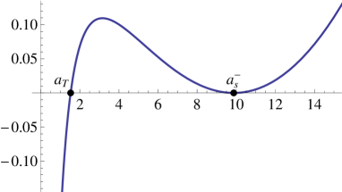
Figure 15: Potential $V(a)$ under the condition $\Lambda=\Lambda^{-}$. A $BB\Rightarrow BC$ universe or a stable ES one is obtained. The constants are chosen as $m=1$, $c_{3}=2.5$, $c_{4}=-4.6$, and $\Lambda=0.195299$. The radii are $a_{T}=1.52772$ and $a_{s}^{-}=9.87298$.

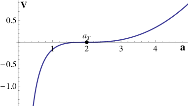
Figure 16: Potential $V(a)$ under the condition $\Lambda=\Lambda^{+}=\Lambda^{-}$. A $BB\Rightarrow BC$ universe is obtained. The constants are chosen as $m=1$, $c_{3}=3$, $c_{4}=-7$, and $\Lambda=0.166667$. The radius is $a_{T}=2$.

V.1.2 two positive roots

We assume $a_{1}<0$, and $a_{2},a_{3}>0$, and set $a_{2}=a_{min}$ and $a_{2}=a_{max}$, so that

$$a_{1}a_{min}a_{max}=\frac{(c_{3}+c_{4})}{(4c_{3}+c_{4}-6+3\Lambda)}<0.$$ (46)

An analysis similar to that in the previous section leads to the conditions for two positive roots and one negative root as follows:

$$c_{3}<2\;,\;\;0<c_{3}+c_{4}<6-3c_{3},$$ (47)

which determine Region 2 of Fig. (12). We find that $\Lambda=\Lambda^{\pm}$ is forbidden since $\Lambda^{+}>-\frac{1}{3}(4c_{3}+c_{4}-6)$ and $\Lambda^{-}<0$ when $c_{3}$ and $c_{4}$ satisfy Eq. (47). This implies that $\Lambda$ is only required to satisfy Eq. (38). Fig. (17) shows the evolution of the potential ${V}(a)$ with the model parameters in Region 2 of Fig. (12). From Fig. (17), we find that an oscillating universe is achieved since $V\leq 0$ in $a\in[a_{min},a_{max}]$ with $V=0$ occurring at $a=a_{min}$ and $a_{max}$.

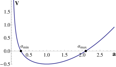
Figure 17: Potential ${V}(a)$ for an oscillating universe with model parameters in Region 2 of Fig. (12). The constants are chosen as $m=1$, $c_{3}=1$, $c_{4}=-0.5$, and $\Lambda=0.5$. The radii are $a_{min}=0.27255$ and $a_{max}=2.10074$.

V.1.3 one positive root

Assuming that $a_{1},a_{2}<0$ and $a_{3}=a_{T}>0$ and using the analysis similar to that in the previous section, we get that the conditions for one positive root

$$1<c_{3}<2\;,\;\;\;\;3-c_{3}-2\sqrt{3-3c_{3}+c_{3}^{2}}<c_{3}+c_{4}<0\;,$$

$$or 2\leq c_{3}<3\;,\;\;\;\;3-2c_{3}<c_{3}+c_{4}<6-3c_{3}\;.$$ (48)

Region 3 of Fig. (12) shows the allowed values of $c_{3}$ and $c_{4}$ for only one positive root. Fig. (18) shows the evolution of the potential ${V}(a)$. It is easy to see that a $BB\rightarrow BC$ universe is realized.

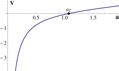
Figure 18: Potential ${V}(a)$ for a $BB\Rightarrow BC$ universe with model parameter in Region 3 of Fig. (12). The constants are chosen as $m=1$, $c_{3}=2.5$, $c_{4}=-4.25$, and $\Lambda=0.06$. and the turning radius is $a_{T}=1.07118$.

V.1.4 no positive root

Since $a_{1},a_{2},a_{3}<0$, and $4c_{3}+c_{4}-6+3\Lambda<0$, one has three inequalities:

$$3-3c_{3}-c_{4}<0,\;\;c_{4}+2c_{3}-1<0,\;\;\;c_{3}+c_{4}>0.$$ (49)

When $c_{3}$ and $c_{4}$ satisfy the above inequalities, $\Lambda^{-}<0$ and $\Lambda^{+}<0$. Therefore, there is no allowed positive value for $\Lambda$. This means that this is not a physically meaningful case.

V.2 $\Lambda>\Lambda^{+}$

This case corresponds to only one real root $a_{3}$. Other two roots $a_{1}$ and $a_{2}$ are a conjugate imaginary pair. Now $\Lambda$ must satisfy

$$Max\;\{0,\Lambda^{+}\}<\Lambda<-\frac{1}{3}(4c_{3}+c_{4}-6)$$ (50)

If this real root $a_{3}$ is negative, then

$$a_{1}a_{2}a_{3}=\frac{(c_{3}+c_{4})}{(4c_{3}+c_{4}-6+3\Lambda)}<0.$$ (51)

Considering the condition of $\Lambda$ (Eq. (50)), we find that there is no solution for Eq. (51). Thus, $a_{3}$ must be a positive one and we set $a_{3}=a_{T}$, which means

$$a_{1}a_{2}a_{T}=\frac{(c_{3}+c_{4})}{(4c_{3}+c_{4}-6+3\Lambda)}>0.$$ (52)

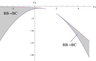
Figure 19: Phase diagram of spacetimes in $(c_{3},c_{4})$ plane when $\Lambda>\Lambda^{+}$. A $BB\Rightarrow BC$ universe is found in the gray region.

Combining Eq. (50) and Eq. (52), we obtain that $c_{3}$ and $c_{4}$ must obey

$$c_{3}<1\;,\;\;\;-(c_{3}-1)^{2}\leq c_{3}+c_{4}<3-c_{3}-2\sqrt{3-3c_{3}+c_{3}^{2}}\;,$$

$$or c_{3}>2\;,\;\;\;-(c_{3}-1)^{2}\leq c_{3}+c_{4}<3-c_{3}-2\sqrt{3-3c_{3}+c_{3}^{2}}\;,$$ (53)

in order to get one positive root and two imaginary roots which are conjugate to each other. In Fig. (19), we show the allowed values of $c_{3}$ and $c_{4}$ for a positive root. Fig. (20) shows the evolution of the potential ${V}(a)$ with the model parameters in the gray regions of Fig. (19), and a $BB\Rightarrow BC$ universe is obtained.

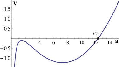
Figure 20: Potential $V(a)$ with model parameters in the gray regions of Fig. (19) and $\Lambda>\Lambda^{+}$. We obtain a $BB\Rightarrow BC$ universe. The constants are chosen as $m=1$, $c_{3}=3$, $c_{4}=-6.75$, and $\Lambda=0.2$. The radius is $a_{T}=12.3248$.

V.3 $\Lambda<\Lambda^{-}$

This case requires

$$0<\Lambda<Min\bigg{\{}\Lambda^{-},-\frac{1}{3}(4c_{3}+c_{4}-6)\bigg{\}}\;.$$ (54)

Under this condition Eq. (51) can’t be satisfied, but Eq. (52) can. Thus, there is also one positive root $a_{3}=a_{T}$ and two conjugate imaginary ones $a_{1}$ and $a_{2}$. Combining the condition on $\Lambda$ given in Eq. (54) and Eq. (52), we get

$$c_{3}>1\;,\;\;-(c_{3}-1)^{2}\leq c_{3}+c_{4}<-\frac{3}{4}(c_{3}-1)^{2}\;.$$ (55)

The allowed region of $c_{3}$ and $c_{4}$ is shown in Fig. (21) and the evolutionary curve of the potential is given in Fig. (22). We find that the potential $V(a)\leq 0$ when $0<a\leq a_{T}$ and the cosmic type is $BB\Rightarrow BC$.

Tab. (2) sums up the results of this section.

Figure 21: Phase diagram of spacetimes in $(c_{3},c_{4})$ plane under the condition $\Lambda<\Lambda^{-}$. A $BB\Rightarrow BC$ universe is found in the gray region.

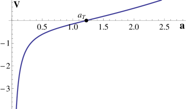
Figure 22: Potential $V(a)$ with model parameters in the gray region of Fig. (21) and $\Lambda<\Lambda^{-}$. We obtain a $BB\Rightarrow BC$ universe. The constants are chosen as $m=1$, $c_{3}=2$, $c_{4}=-2.85$, and $\Lambda=0.15$. The radius is $a_{T}=1.22118$

Table 2: Summary of the cosmic type in the $4c_{3}+c_{4}-6+3\Lambda<0$ case

$\Lambda$	$c_{3},\;c_{4}$	Cosmic Type
	$c_{3}<1,\;\;-\frac{3}{4}(c_{3}-1)^{2}<c_{3}+c_{4}<0$	$BB\Rightarrow BC$
	$2<c_{3}\leq 3,\;\;-(c_{3}-1)^{2}<c_{3}+c_{4}<3-2c_{3}$	or Oscillation
$Max\;\{\Lambda^{-},0\}<\Lambda<$	$or~{}c_{3}>3,\;\;-(c_{3}-1)^{2}<c_{3}+c_{4}<6-3c_{3}$
$Min\{-\frac{1}{3}(4c_{3}+c_{4}+6),\Lambda^{+}\}$	$c_{3}<2,\;\;0<c_{3}+c_{4}<6-3c_{3}$	Oscillation
	$1<c_{3}<2,\;3-c_{3}-2\sqrt{3-3c_{3}+c_{3}^{2}}<c_{3}+c_{4}<0$	$BB\Rightarrow BC$
	$or~{}2\leq c_{3}<3,\;\;\;\;3-2c_{3}<c_{3}+c_{4}<6-3c_{3}$
	$c_{3}<1,\;-\frac{3}{4}(c_{3}-1)^{2}<c_{3}+c_{4}$
$0<\Lambda=\Lambda^{+}<$	$<3-c_{3}-2\sqrt{3-3c_{3}+c_{3}^{2}}$	$BB\Rightarrow BC$
$-\frac{1}{3}(4c_{3}+c_{4}+6)$	$or~{}c_{3}>2,-(c_{3}-1)^{2}\leq c_{3}+c_{4}$	Unstable ES
	$<3-c_{3}-2\sqrt{3-3c_{3}+c_{3}^{2}}$
$0<\Lambda=\Lambda^{-}<$	$2<c_{3}\leq 3,\;\;-(c_{3}-1)^{2}\leq c_{3}+c_{4}<3-2c_{3}$	$BB\Rightarrow BC$
$-\frac{1}{3}(4c_{3}+c_{4}-6)$	$or~{}c_{3}>3,\;-(c_{3}-1)^{2}\leq c_{3}+c_{4}<-\frac{3}{4}(c_{3}-1)^{2}$	Stable ES
$\Lambda=\Lambda^{-}=\Lambda^{+}=\frac{1}{3(c_{3}-1)}$	$c_{3}>2,\;\;c_{3}+c_{4}=-(c_{3}-1)^{2}$	$BB\Rightarrow BC$
	$c_{3}<1,\;\;-(c_{3}-1)^{2}\leq c_{3}+c_{4}$
$Max\;\{0,\Lambda^{+}\}<\Lambda<$	$<3-c_{3}-2\sqrt{3-3c_{3}+c_{3}^{2}}$	$BB\Rightarrow BC$
$-\frac{1}{3}(4c_{3}+c_{4}-6)$	$or~{}c_{3}>2,\;\;-(c_{3}-1)^{2}\leq c_{3}+c_{4}$
	$<3-c_{3}-2\sqrt{3-3c_{3}+c_{3}^{2}}$
$0<\Lambda<$	$c_{3}>1,\;\;-(c_{3}-1)^{2}\leq c_{3}+c_{4}<-\frac{3}{4}(c_{3}-1)^{2}$	$BB\Rightarrow BC$
$Min\big{\{}\Lambda^{-},-\frac{1}{3}(4c_{3}+c_{4}-6)\big{\}}$

VI The case of $\Lambda=-\frac{1}{3}(4c_{3}+c_{4}-6)$

In this case Eq. (II) becomes

$$V(a)=\frac{m^{2}}{a}\bigg{[}-(3-3c_{3}-c_{4})a^{2}-(c_{4}+2c_{3}-1)a+\frac{1}{3}(c_{3}+c_{4})\bigg{]}\;.$$ (56)

Apparently, $V(a)=0$ has two roots:

$$a_{1}=\frac{3-6c_{3}-3c_{4}-\sqrt{3(3+6c_{4}-4c_{3}c_{4}-c_{4}^{2})}}{-6(3-3c_{3}-c_{4})}$$

$$a_{2}=\frac{3-6c_{3}-3c_{4}+\sqrt{3(3+6c_{4}-4c_{3}c_{4}-c_{4}^{2})}}{-6(3-3c_{3}-c_{4})}$$ (57)

Now we divide our discussion into two cases, i.e., $-(3-3c_{3}-c_{4})>0$ and $-(3-3c_{3}-c_{4})<0$.

VI.1 $-(3-3c_{3}-c_{4})>0$

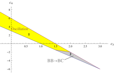
Figure 23: Phase diagram of spacetimes in $(c_{3},c_{4})$ plane under the condition $\Lambda=-\frac{1}{3}(4c_{3}+c_{4}-6)$ and $-(3-3c_{3}-c_{4})>0$. An oscillating universe is found in Region 1, and a $BB\Rightarrow BC$ one is obtained in Region 2.

If two roots are all positive, we set $a_{2}=a_{min}$ and $a_{3}=a_{max}$, and find that $c_{3}$ and $c_{4}$ must satisfy $\Delta=(3+c_{4}(6-4c_{3})-c_{4}^{2})>0$, $c_{3}+c_{4}>0$, $-(3-3c_{3}-c_{4})>0$, $\Lambda=-\frac{1}{3}(4c_{3}+c_{4}-6)>0$, and $-(c_{4}+2c_{3}-1)<0$. These lead to

$$c_{3}\leq\frac{3}{2}\;,\;\;3-2c_{3}<c_{3}+c_{4}<6-3c_{3}\;,$$

$$or \frac{3}{2}<c_{3}<2\;,\;\;0<c_{3}+c_{4}<6-3c_{3}\;,$$ (58)

which is represented as Region 1 in Fig. (23) where the phase diagram of spacetimes in $(c_{3},c_{4})$ plane is shown. Fig. (24) displays the evolution of the potential with model parameters in Region 1 of Fig. (23). We can see that $V(a)\leq 0$ in $a\in[a_{min},a_{max}]$ with the equality holding at $a=a_{min}$ and $a=a_{max}$. Thus, an oscillating universe is obtained.

If $a_{1}=a_{2}$, then $c_{4}=3-2c_{3}\pm 2\sqrt{3+c_{3}(c_{3}-3)}$, which is outside Region 1 of Fig. (23). Thus, a stable static Einstein universe can’t be obtained in this case.

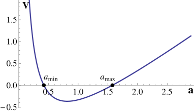
Figure 24: Potential ${V}(a)$ with model parameters in Region 1 of Fig. (23). An oscillating universe is obtained. The constants are chosen as $m=1$, $c_{3}=1$, $c_{4}=1$, and $\Lambda=\frac{1}{3}$. The radii are $a_{min}=0.42265$ and $a_{max}=1.57735$.

Now we consider the case of $a_{1}<0$ and $a_{2}=a_{T}>0$. We find that there is a $BB\Rightarrow BC$ cosmic evolution type as shown in Fig. (25), and $c_{3}$ and $c_{4}$ satisfy

$$\frac{3}{2}<c_{3}\leq 2\;,\;\;3-2c_{3}<c_{3}+c_{4}<0\;,$$

$$or 2<c_{3}<3\;,\;\;3-2c_{3}<c_{3}+c_{4}<6-3c_{3}\;,$$ (59)

which correspond to Region 2 in Fig. (23).

If both $a_{1}$ and $a_{2}$ are negative, then $V(a)>0$ in $a\in(0,\infty)$. So this is not a case of physical significance.

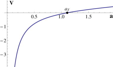
Figure 25: Potential ${V}(a)$ with model parameters in Region 2 of Fig. (23). A $BB\Rightarrow BC$ universe is obtained. The constants are chosen as $m=1$, $c_{3}=2.5$, $c_{4}=-4.25$, and $\Lambda=0.083333$. and the turning radius is $a_{T}=1.10728$.

VI.2 $-(3-3c_{3}-c_{4})<0$

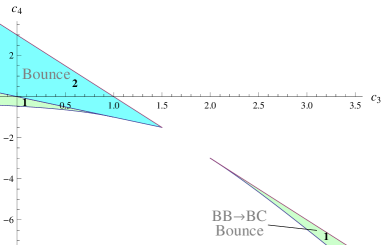
Figure 26: Phase diagram of spacetimes in $(c_{3},c_{4})$ plane under the conditions $\Lambda=-\frac{1}{3}(4c_{3}+c_{4}-6)$ and $-(3-3c_{3}-c_{4})<0$. A bouncing universe is found in Regions 1 and 2, and a $BB\Rightarrow BC$ universe is obtained in Region 1.

Since $a_{1}>0$ and $a_{2}>0$ require $\Delta=\frac{1}{3}(3+c_{4}(6-4c_{3})-c_{4}^{2})>0$, $c_{3}+c_{4}<0$, and $-(c_{4}+2c_{3}-1)>0$, the conditions for two positive roots are

$$c_{3}<1\;,\;\;3-c_{3}-2\sqrt{3-3c_{3}+c_{3}^{2}}<c_{3}+c_{4}<0\;,$$

$$2<c_{3}\leq 3\;,\;\;3-c_{3}-2\sqrt{3-3c_{3}+c_{3}^{2}}<c_{3}+c_{4}<3-2c_{3}\;,$$

$$or c_{3}>3\;,\;\;3-c_{3}-2\sqrt{3-3c_{3}+c_{3}^{2}}<c_{3}+c_{4}<6-3c_{3}\;.$$ (60)

In Region 1 of Fig. (26), we show the allowed values $c_{3}$ and $c_{4}$ for two positive roots. Setting $a_{1}=a_{T2}$ and $a_{2}=a_{T1}$ since $a_{1}>a_{2}$, we show the evolution of the potential ${V}(a)$ in Fig. (27) with the model parameters in Region 1 of Fig. (26). From this figure, we see that a $BB\Rightarrow BC$ universe or a bouncing one is obtained since $V\leq 0$ in $a\in(0,a_{T1}]$ and $[a_{T2},\infty)$ with $V=0$ occurring at $a=a_{T1}$ and $a=a_{T2}$. Another possibility is that the universe starts at the big bang singularity and, rather than bounce back, it quantum mechanically tunnels to $a_{T1}$ when it evolves to $a_{T2}$ and then expands forever.

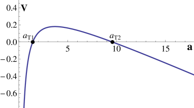
Figure 27: Potential ${V}(a)$ with model parameters in Region 1 of Fig. (26). A $BB\Rightarrow BC$ universe or a bouncing one is found. The constants are chosen as $m=1$, $c_{3}=2.5$, $c_{4}=-4.55$, and $\Lambda=0.183333$. The radii are $a_{T1}=1.42774$ and $a_{T2}=9.57226$.

If $c_{4}=3-2c_{3}\pm 2\sqrt{3+c_{3}(c_{3}-3)}$, it is easy to see $a_{1}=a_{2}$, which means that $V(a)=0$ has a double solution $a_{s}$

$$a_{s}=\frac{-3+2c_{3}+2\sqrt{3+c_{3}(c_{3}-3)}}{3(c_{3}-2)}\;.$$ (61)

We find that $a_{s}$ is an unstable ES universe and it exists under the conditions

$$c_{3}<1\;,\;\;c_{3}+c_{4}=3-c_{3}-2\sqrt{3+c_{3}(c_{3}-3)}\;,$$

$$or c_{3}>2\;,\;\;c_{3}+c_{4}=3-c_{3}-2\sqrt{3+c_{3}(c_{3}-3)}\;.$$ (62)

Thus, as shown in Fig (28), if the universe initiates from big bang, it will expand to an unstable ES universe and then turn over or expand forever.

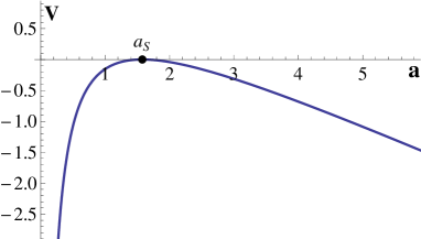
Figure 28: Potential $V(a)$ with model parameters satisfying Eq. (63). An unstable Einstein static state universe is obtained. The constants are chosen as $m=1$, $c_{3}=3$, $c_{4}=-4.64575$, and $\Lambda=0.15470$. $a_{s}=1.57735$.

Now we consider the case of $a_{2}<0$ and $a_{1}=a_{T}>0$. In this case, a bouncing universe is obtained, as shown in Fig. (29), if $c_{3}$ and $c_{4}$ satisfy

$$c_{3}<\frac{3}{2}\;,\;\;0<c_{3}+c_{4}<3-2c_{3},$$ (63)

which corresponds to Region $2$ of Fig. (26).

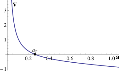
Figure 29: Potential $V(a)$ with model parameters in Region 1 of Fig. (26). A bouncing universe is found. The constants are chosen as $m=1$, $c_{3}=1$, $c_{4}=-0.5$, and $\Lambda=0.83333$. The turning radius at a bounce is $a_{T}=0.263763$.

If both $a_{1}$ and $a_{2}$ are not positive, we find that the potential is always negative as shown in Fig. (30) and the cosmic type is $BB\Rightarrow\infty$ or $\infty\Rightarrow BC$.

The results of this section are summed up in Tab. (3).

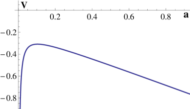
Figure 30: Potential ${V}(a)$ for the case of without positive root. A $BB\Rightarrow\infty$ or $\infty\Rightarrow BC$ one is obtained. The constants are chosen as $m=1$, $c_{3}=1.2$, $c_{4}=-1.22$, and $\Lambda=0.806667$.

Table 3: Summary of the cosmic type in the $4c_{3}+c_{4}-6+3\Lambda=0$ case

$c_{3},\;c_{4}$	Cosmic Type
$c_{3}\leq\frac{3}{2},\;\;3-2c_{3}<c_{3}+c_{4}<6-3c_{3}$	Oscillation
$or~{}\frac{3}{2}<c_{3}<2,\;\;0<c_{3}+c_{4}<6-3c_{3}$
$\frac{3}{2}<c_{3}\leq 2,\;\;3-2c_{3}<c_{3}+c_{4}<0$	$BB\Rightarrow BC$
$or~{}2<c_{3}<3,\;\;3-2c_{3}<c_{3}+c_{4}<6-3c_{3}$
$c_{3}<1,\;\;3-c_{3}-2\sqrt{3-3c_{3}+c_{3}^{2}}<c_{3}+c_{4}<0$	$BB\Rightarrow BC$
$2<c_{3}\leq 3,\;\;3-c_{3}-2\sqrt{3-3c_{3}+c_{3}^{2}}<c_{3}+c_{4}<3-2c_{3}$	or Bounce
$or~{}c_{3}>3,\;\;3-c_{3}-2\sqrt{3-3c_{3}+c_{3}^{2}}<c_{3}+c_{4}<6-3c_{3}$
	$BB\Rightarrow BC$
$c_{3}<1,\;\;c_{3}+c_{4}=3-c_{3}-2\sqrt{3+c_{3}(c_{3}-3)}$	$BB\Rightarrow\infty$
$or~{}c_{3}>2,\;\;c_{3}+c_{4}=3-c_{3}-2\sqrt{3+c_{3}(c_{3}-3)}$	$\infty\Rightarrow BC$
	or Bounce
	Unstable ES
$c_{3}<\frac{3}{2},\;\;0<c_{3}+c_{4}<3-2c_{3},$	Bounce

VII Conclusions

Massive gravity is a modification of general relativity. It has been spurring an increasing deal of interest recently, since it can explain the present accelerated cosmic expansion without the need of dark energy. In this paper, using a method in which the scale factor $a$ changes as a particle in a “potential”, we analyze all possible cosmic evolutions in a ghost-free massive gravity theory. A spatially flat universe is considered in our discussion and we assume that the vacuum energy is the only energy component. The results are summed up in Tabs. (1, 2, 3). We find that there may exist an oscillating universe between $a_{min}$ and $a_{max\;}$ or a bouncing one at $a_{T}$ if model parameters are in some specific regions. If the cosmic scale factor is in the region $[a_{min},a_{max\;}]$ initially, the universe may undergo an oscillation. After a number of oscillations, it may evolve to the bounce point $a_{T}$ through quantum tunneling. While, if the universe contracts initially from an infinite scale, it can turn around at $a_{T}$ and then expand forever. Thus, the big bang singularity problem can be resolved successfully. Remarkably, although we do have a stable ES solution in some circumstances, the universe can not stay at this stable state past-eternally since it is allowed to quantum mechanically tunnel to a big-bang-to-big-crunch cosmic evolution type and end with a big crunch. Thus, the existence of a stable ES universe can not successfully resolve the big bang singularity in the massive gravity. This feature is related to the behavior of $V(a)\rightarrow-\infty$ as $a\rightarrow 0$, which is a result of $c_{3}+c_{4}<0$ in the massive gravity we consider in the present paper, when there exists a stable ES universe with a finite $a_{s}$. Let us note however that both in the Horava-Lifshitz gravity Maeda2010 and the DGP braneworld scenario Zhang2012 , there exist stable ES universes where $V(a)\rightarrow\infty$ as $a\rightarrow 0$, so a quantum tunneling to the big bang singularity is not allowed ( refer to Fig. (4) in Maeda2010 and Fig. (5) in Zhang2012 ) and as a result the existence of a stable ES universe can avoid the big bang singularity in these theories. Therefore, whether the existence of a stable ES universe can resolve the big bang singularity or not is a peculiar feature of the theory of gravity itself and it is in fact determined by the behavior of the leading term in $V(a)$ as $a$ approaches zero, i.e., the big bang singularity.

- (1) S. Perlmutter, et al., Astrophys. J. 517 (1999) 565.
- (2) A. G. Riess, et al., Astron. J. 116 (1998) 1009.
- (3) D. N. Spergel, et al., Astrophys. J. Suppl. 148 (2003) 175; D. N. Spergel, et al., Astrophys. J. Suppl. 170 (2007) 377.
- (4) D. J. Eisenstein, et al., Astron. J. 633 (2005) 560.
- (5) M. Tegmark, et al., Phys. Rev. D 69 (2004) 103501.
- (6) D. Dvali, G. Gabadadze and M. Porrati, Phys. Lett. B 485 (2000) 208.
- (7) M. Fierz and W. Pauli, Proc. Roy. Soc. Lond. A 173 (1939) 211.
- (8) H. van Dam and M. J. G. Veltman, Nucl. Phys. B 22 (1970) 397; V. I. Zakharov, JETP Lett. 12 (1970) 312.
- (9) A. I. Vainshtein, Phys. Lett. B 39 (1972) 393.
- (10) D.G. Boulware and S. Deser, Phys. Rev. D 6 (1972) 3368.
- (11) N. Arkani-Hamed, H. Georgi and M. D. Schwartz, Annals Phys. 305 (2003) 96; P. Creminelli, A. Nicolis, M. Papucci and E. Trincherini, JHEP 0509 (2005) 003; C. Deffayet and J. W. Rombouts, Phys. Rev. D 72 (2005) 044003; G. Gabadadze and A. Gruzinov, Phys. Rev. D 72 (2005) 124007.
- (12) C. de Rham, G. Gabadadze, Phys. Rev. D 82 (2010) 044020; C. de Rham, G. Gabadadze and A. J. Tolley, Phys. Rev. Lett. 106 (2011) 231101.
- (13) S. Deser and A. Waldron, arXiv:1212.5835.
- (14) G. D Amico, C. de Rham, S. Dubovsky, G. Gabadadze, D. Pirtskhalava and A. J. Tolley, Phys. Rev. D 84 (2011) 124046; A. E. Gumrukcuoglu, C. Lin and S. Mukohyama, JCAP 1111 (2011) 030; A. E. Gumrukcuoglu, C. Lin and S. Mukohyama, JCAP 1203 (2012) 006; A. De Felice, A. E. Gumrukcuoglu and S. Mukohyama, Phys. Rev. Lett. 109 (2012) 171101; A. E. Gumrukcuoglu, C. Lin and S. Mukohyama, Phys. Lett. B717 (2012) 295; K. Koyama, G. Niz and G. Tasinato, JHEP 1112 (2011) 065; D. Comelli, M. Crisostomi, F. Nesti and L. Pilo, JHEP 1203 (2012) 067 [Erratum-ibid. 1206 (2012) 020]; M. Crisostomi, D. Comelli and L. Pilo, JHEP 1206 (2012) 085; P. Gratia, W. Hu and M. Wyman, Phys. Rev. D 86 (2012) 061504; T. Kobayashi, M. Siino, M. Yamaguchi and D. Yoshida, Phys. Rev. D 86 (2012) 061505; G. D Amico, arXiv:1206.3617; M. Fasiello and A. J. Tolley, JCAP 1211 (2012) 035; G. D Amico, G. Gabadadze, L. Hui and D. Pirtskhalava, arXiv:1206.4253; D. Langlois and A. Naruko, Class. Quant. Grav. 29 (2012) 202001; Y. Gong, arXiv: Commun. Theor. Phys. 59, 319 (2013); Q. G. Huang, Y. S. Piao and S. Y. Zhou, arXiv: 1206.5678; E. N. Saridakis, arXiv: 1207.1800 [gr-qc]; Y. F. Cai, C. Gao and E. N. Saridakis, JCAP 1210 (2012) 048; C. I. Chiang, K. Izumi and P. Chen, arXiv: 1208.1222.
- (15) V. F. Cardone, N. Radicella and L. Parisi, Phys. Rev. D 85 (2012) 124005; Y. Gong, arXiv:1210.5396.
- (16) L. Parisi, N. Radicella, and G. Vilasi, Phys.Rev. D 86 (2012) 024035.
- (17) Y. Zhang, R. Saito, and M. Sasaki, J. Cosmol. Astropart. Phys. 02 (2013) 029.
- (18) K. Maeda, Y. Misonoh, T. Kobayashi, Phys. Rev. D 82 (2010) 064024.
- (19) K. Zhang, P. Wu and H. Yu, Phys. Rev. D 85 (2012) 043521.
- (20) A. H. Chamseddine and V. Mukhanov, JHEP 8 (2011) 91; T. M. Nieuwenhuizen, Phys. Rev. D 84 (2011) 024038.
- (21) A. H. Chamseddine and M. S. Volkov, Phys. Lett. B 704 (2011) 652.
- (22) B. Vakili and N. Khosravi, Phys. Rev. D 85 (2012) 083529.