Quasi-Monte Carlo methods for lattice systems:
a first look

Abstract

We investigate the applicability of Quasi-Monte Carlo methods to Euclidean lattice systems for quantum mechanics in order to improve the asymptotic error behavior of observables for such theories. In most cases the error of an observable calculated by averaging over random observations generated from an ordinary Markov chain Monte Carlo simulation behaves like $N^{-1/2}$, where $N$ is the number of observations. By means of Quasi-Monte Carlo methods it is possible to improve this behavior for certain problems to $N^{-1}$, or even further if the problems are regular enough. We adapted and applied this approach to simple systems like the quantum harmonic and anharmonic oscillator and verified an improved error scaling.

15(29,2) HU-EP-13/05
SFB/CPP-13-13
DESY 13-022

1 Introduction

Markov chain-Monte Carlo (Mc-MC) techniques are commonly the method of choice for the numerical evaluation of partition functions in statistical physics or path integrals in Euclidean time for models in high energy physics. The reason is that they are based on importance sampling and hence select the integration points automatically according to the corresponding weight in the integrand. Many algorithms have been developed to implement a Mc-MC, starting from the Metropolis algorithm, heatbath and over-relaxation to cluster and hybrid Monte Carlo algorithms, see e.g. refs. [1, 2]. In this way, simulations of demanding 4-dimensional quantum field theories became possible and, in fact, were carried out very successfully to e.g. compute the low-lying hadron spectrum [3] or deriving bounds for the Higgs boson mass [4].

The drawback of Mc-MC is that it estimates the desired quantity stochastically and hence the results are affected by a statistical error which sometimes needs very long and computer time extensive samplings. Quantitatively, this sampling error behaves as $N^{-1/2}$ for a (thermalized) sample size of $N$. This error scaling behaviour is often a real stumbling block in such Mc-MC simulations. If we consider lattice quantum chromodynamics as a typical system for Mc-MC calculations in high energy physics, then due to this error scaling and the very high computational demand of these simulations, it is often impossible to significantly decrease the error to the targeted precision. It would therefore be very desirable to have Monte Carlo methods available that possibly show a better error scaling.

Such methods in fact exist in form of Quasi-Monte Carlo (QMC) techniques [5],[6], where it is known that the error scaling can be improved to an $N^{-1}$, or even more if the problem exhibits enough structure (smoothness, periodicity). QMC methods have been analyzed theoretically very thoroughly and comprehensively, and many successful applications in mathematical finance based on high-dimensional Gaussian integrals have been studied in the last two decades [7],[8]. On the other hand, to the best of our knowledge, QMC methods were never tested successfully in high-dimensional models that are relevant for high energy physics.

In this paper we therefore want to perform a very first step towards the very challenging goal of applying QMC methods to generic field theories by looking at the non-trivial case of the anharmonic quantum mechanical oscillator discretized on a finite Euclidean time lattice and evaluated in the corresponding path integral formulation [9]. For the case of the anharmonic oscillator the system is not Gaussian anymore and a successful application of QMC methods would be a first non-trivial test. Of course, even if such a test is successful, there is a long way to address eventually 4-dimensional quantum field theories, but a proof of concept would certainly open the promising road to attack field theories in the future.

We will start our discussion with a description of the harmonic oscillator in its time-discretized path integral formulation. Here the problem is fully Gaussian and the application of adequate QMC methods should lead to an improved error scaling, an expectation that we will see to be fulfilled. Nevertheless, the harmonic oscillator example can serve well to explain how QMC methods work and how an improved error scaling behaviour is realized.

We will then proceed to look at the anharmonic oscillator and we will demonstrate that also in this case QMC leads to an improved error scaling, although the obtained rate of convergence is still not optimal and leaves space for improvements. We consider this, nevertheless, to be a very promising non-trivial result which bears the potential that also other models in quantum mechanics, e.g. the topological quantum mechanical action of ref. [10] and even field theories can be evaluated by QMC methods. For a first account of our studies, we refer to the proceedings contribution of ref. [11].

2 Quantum Mechanical Harmonic and Anharmonic Oscillator

In this section we will discuss the basic steps for the quantization of the theory in the path integral approach and the discretization on a time lattice. The first step is the construction of the Lagrangian (resp. the action) of the corresponding classical mechanical system for a given path $x(t)$ of a particle with mass $M_{0}$. For a numerically stable evaluation of the path integral it is essential to pass on to Euclidean time. In this case the Lagrangian $L$ and the action $S$ is given by:

$$L(x,t) =\frac{M_{0}}{2}\left(\frac{dx}{dt}\right)^{2}+V(x)$$ (1)

$$S(x) =\int_{0}^{T}\,L(x,t)\;dt.$$ (2)

Depending on the scenario (harmonic or anharmonic oscillator) the potential $V(x)$ consists of two parts

$$V(x)=\underbrace{\frac{\mu^{2}}{2}x^{2}}_{\text{harmonic part}}+\underbrace{\lambda\,x^{4}}_{\text{anharmonic part}}\;,$$ (3)

such that the parameter $\lambda$ controls the anharmonic part of the theory. It should also be mentioned that in the anharmonic case the parameter $\mu^{2}$ can take on negative values, leading then to a double well potential.

The next step is to discretize time into equidistant time slices with a spacing of $a$. The path is then only defined on the time slices:

$$t \rightarrow t_{i}=(i-1)\cdot a\quad i=1\ldots d$$ (4)

$$x(t) \rightarrow x_{i}=x(t_{i})\;.$$ (5)

On the lattice the derivative with respect to the time appearing in (1) (first term) will be replaced by the forward finite difference $\nabla x_{i}=\frac{1}{a}(x_{i+1}-x_{i})$. The choice of the lattice derivative is not unique and requires special care, particularly if one considers more complicated models like lattice QCD. But in [9] it was shown that the lattice derivative chosen here permits a well defined continuum limit. Putting all the ingredients together, we can write down the lattice action for the (an)harmonic oscillator

$$S^{\text{latt}}(\mathbf{x})=a\sum_{i=1}^{d}\left(\frac{M_{0}}{2}\left(\nabla x_{i}\right)^{2}+V(x_{i})\right)\;.$$ (6)

For the path a cyclic boundary condition $x_{d+1}=x_{1}$ can be assumed. In the following the superscript “latt” will be dropped, as we will only refer to the lattice action from now on. The expectation value of an observable $O$ of the quantized theory expressed in terms of the path integral reads as follows:

$$\left\langle O(\mathbf{x})\right\rangle\,=\,\frac{\int_{\mathbb{R}^{d}}O(\mathbf{x})e^{-S(\mathbf{x})}dx_{1}...dx_{d}}{\int_{\mathbb{R}^{d}}e^{-S(\mathbf{x})}dx_{1}...dx_{d}}\;.$$ (7)

This expression is suitable for a numerical evaluation of certain quantities of the underlying theory. Up to now only Monte Carlo methods are known to give reliable results for dimensions $d\gg 10$. One type of such methods, often used in physics, is the Markov chain-Monte Carlo approach mostly applying the weight $\propto e^{-S(\mathbf{x})}$ for sampling paths $\{x_{i}\}$ (so-called “importance sampling”). In the next sections, we will provide a summary of the mathematical results for QMC methods (and their randomizations), and particularly recapitulate in a rather mathematical language the strict error scaling bounds for this methods. The reader more interested directly in the results may move to section 7 directly.

3 Direct Monte Carlo and Quasi–Monte Carlo methods

We provide in this and the following sections 3-7 some mathematical background of QMC methods. The reader who is more interested in our results, may proceed directly to section 8. In many practical applications one is interested in calculating quotients of the form (7) where the action $S(.)$ and the observables $O(.)$ are usually smooth functions in high dimensions. In some special situations where one would like to deal with integrands of moderately high dimensions, one possible approach is to consider estimators $\hat{I}_{1}$,$\hat{I}_{2}$ for the integrals $I_{1}$,$I_{2}$ in the numerator and in the denominator of (7) separately, and then take $\hat{I}_{1}/\hat{I}_{2}$ as an estimation of $\left\langle O(\mathbf{x})\right\rangle$. Another possible approach one can consider is given by the so-called weighted uniform sampling (WUS) estimator, analyzed in [12]. In the latter case, one takes a joint estimator for the total quantity $\left\langle O(\mathbf{x})\right\rangle$, using a single direct sampling method. We will show some characteristics of the WUS estimator in section 7, and we will refer from now on to the latter two approaches as direct sampling methods for estimating (7). In many interesting examples, we encounter the case were the action $S(.)$ and the observable $O(.)$ lead to integrals $I_{1}$,$I_{2}$ of Gaussian type. Then the integrals $I_{1}$,$I_{2}$ can be written in the form

$$I_{i}\>=\>\frac{1}{(2\pi)^{d/2}\sqrt{\det(C)}}\int_{\mathbb{R}^{d}}g_{i}(\mathbf{x})e^{-\frac{1}{2}\mathbf{x}^{\top}C^{-1}\mathbf{x}}d\mathbf{x},\quad\mathbf{x}=(x_{1},\dots,x_{d}),\;i=1,2\quad,$$

where $C$ denotes the covariance matrix of the Gaussian density function. A transformation to the unit cube in $\mathbb{R}^{d}$ can be applied such that the corresponding integrals take the form

$$I\>=\>\int_{[0,1]^{d}}g(A{\boldsymbol{\Phi}}^{-1}({\boldsymbol{z}}))d{\boldsymbol{z}}\>=\>\int_{[0,1]^{d}}f({\boldsymbol{z}})d{\boldsymbol{z}}\>=\>I_{[0,1]^{d}}(f),\quad{\boldsymbol{z}}=(z_{1},\dots,z_{d})\,.$$ (8)

Here $AA^{\top}=C$ is some symmetric factorization of the covariance matrix, and ${\boldsymbol{\Phi}}^{-1}({\boldsymbol{z}}):=(\Phi^{-1}(z_{1}),\dots,\Phi^{-1}(z_{d}))^{\top}$, where $\Phi^{-1}({\cdot})$ represents the inverse of the normal cumulative distribution function $\Phi({\cdot})$.
In the classical direct Monte–Carlo (MC) approach one tries to estimate (8) by generating samples pseudo-randomly. One starts with a finite sequence of independent identically distributed (i.i.d.) samples $P_{N}=\{{\boldsymbol{z}}_{1},\dots,{\boldsymbol{z}}_{N}\}$, where the points ${\boldsymbol{z}}_{j},\;1\leq j\leq N$, have been generated from the uniform distribution in $[0,1]^{d}$. Then, the quadrature rule is fixed by taking the average of the function evaluations for $f$

$$Q_{N}:=\frac{1}{N}\sum_{j=1}^{N}f({\boldsymbol{z}}_{j}),$$

as an approximation of the desired integral $\int_{[0,1]^{d}}f({\boldsymbol{z}})\;d{\boldsymbol{z}}$. The resulting estimator $\hat{Q}_{N}$ is unbiased. The integration error can be approximated via the central limit theorem, given that $f$ belongs to $L_{2}([0,1]^{d})$. The variance of the estimator $\hat{Q}_{N}$ is given by

$$\frac{\sigma^{2}}{N}=\frac{1}{N}\left(\int_{[0,1]^{d}}f^{2}({\boldsymbol{z}})\;d{\boldsymbol{z}}-\left(\int_{[0,1]^{d}}f({\boldsymbol{z}})\;d{\boldsymbol{z}}\right)^{2}\right).$$

As measured by its standard deviation from zero the integration error associated with the MC approach is then of order $O(N^{-1/2})$. The quality of the MC samples relies on the selected pseudo–random number generators of uniform samples, here we use the Mersenne Twister generator from Matsumoto and Nishimura (see [13]). MC is in general a very reliable tool in high–dimensional integration, but the order of convergence is in fact rather poor.

In contrast, QMC methods generates deterministically point sets that are more regularly distributed than the pseudo–random points from MC (see [5], [14], [15], [6]). Typical examples of QMC are shifted lattice rules and low-discrepancy sequences. In order to give a short introduction to the subject, we define now the classical notion of discrepancy of a finite sequence of points $P_{N}$ in $[0,1)^{d}$. Given $P_{N}=\{{\boldsymbol{z}}_{1},\dots,{\boldsymbol{z}}_{N}\}$ a set of points in $[0,1)^{d}$, and a nonempty family $\mathbb{I}$ of Lebesgue-measurable sets in $[0,1)^{d}$, we define the classical discrepancy function by

$$D(\mathbb{I};P_{N}):=\sup_{B\in\mathbb{I}}\left|\frac{\sum_{i=1}^{N}\>c_{B}({\boldsymbol{z}}_{i})}{N}-\lambda_{d}(B)\right|,$$

where $c_{B}$ is the characteristic function of $B$, and $\lambda_{d}$ is the Lebesgue measure in $\mathbb{R}^{d}$. This allows us to define the so-called star discrepancy

Definition 3.1

We define the star discrepancy $D^{\star}(P_{N})$ of the point set $P_{N}$ by $D^{\star}(P_{N}):=D(\mathbb{I};P_{N})$, where $\mathbb{I}$ is the family of all sub-intervals of the form $\prod_{i=1}^{d}[0,u_{i})$, with $u_{i}\geq 0,\;1\leq i\leq d$.

The star discrepancy can be considered as a measure of the worst difference between the uniform distribution and the sampled distribution in $[0,1)^{d}$ attributed to the point set $P_{N}$. The usual way to analyze QMC as a deterministic method is by choosing a class of integrand functions $F$, and a measure of discrepancy $D(P_{N})$ for the point sets $P_{N}$. Then, the deterministic integration error is usually given in the form

$$|Q_{N}-\int_{[0,1]^{d}}f({\boldsymbol{z}})\;d{\boldsymbol{z}}|\;\;\leq\;D(P_{N})V(f),$$

where $V(f)$ measures a particular variation of the function $f\in F$. A classical particular error bound in this form is the famous Koksma–Hlawka inequality, where $D(P_{N})$ is taken to be the star discrepancy of the point set $P_{N}$, and $V(f)$ is the variation in the sense of Hardy and Krause of $f$.

In the context of QMC, a sequence of points ${\boldsymbol{z}}_{1},{\boldsymbol{z}}_{2},...$ in $[0,1)^{d}$ is called a low-discrepancy sequence if

$$D^{\star}(\{{\boldsymbol{z}}_{1},\dots,{\boldsymbol{z}}_{N}\})=O(N^{-1}(\log(N))^{d}).$$ (9)

An important part of QMC constructions satisfying this asymptotic bound are known under the name of $(t,d)$-sequences and will be discussed in more detail in section 4. For moderate values of $N$, the influence of the logarithmic term in (9) usually can not be ignored (see $5.7$ and $5.8$ in [16]), because the term $N^{-1}(\log(N))^{d}$ grows until $N>2^{d}$. This normally prevents a straightforward use of low-discrepancy sequences in practical situations with very large dimensions. The latter situations are typically very high-dimensional integration problems where all variables and interactions between variables are equally important.

The practical success of QMC sequences in very high-dimensional integration problems with enough smoothness usually relies in an appropriate combination with an effective-dimension reduction transformation. We will discuss the analysis of effective-dimensions more in detail in 6. Well investigated settings for the integration error analysis of functions exhibiting a concentration of importance in few variables or groups of few variables are the so-called weighted reproducing kernel Hilbert spaces (see [14]), which will be considered briefly in the following section.

3.1 Quasi–Monte Carlo errors and complexity

For error analysis of QMC methods, there are certain reproducing kernel Hilbert spaces $\mathbb{F}_{d}$ of functions $f:[0,1]^{d}\to\mathbb{R}$ that are particularly useful (see [17]). Let us denote now with $\langle\cdot,\cdot\rangle$ and $\|\cdot\|$ the inner product and norm in $\mathbb{F}_{d}$. A reproducing kernel is a function $K:[0,1]^{d}\times[0,1]^{d}\to\mathbb{R}$ satisfying the properties

1. $K(\cdot,{\boldsymbol{y}})\in\mathbb{F}_{d}$ for each ${\boldsymbol{y}}\in[0,1]^{d}$

2. $\langle f,K(\cdot,{\boldsymbol{y}})\rangle=f({\boldsymbol{y}})$ for each ${\boldsymbol{y}}\in[0,1]^{d}$ and $f\in\mathbb{F}_{d}$

If the integral

$$I(f)=\int_{[0,1]^{d}}f({\boldsymbol{z}})d{\boldsymbol{z}}$$

is a continuous functional on the space $\mathbb{F}_{d}$, then the worst case quadrature error

$$e_{N}(\mathbb{F}_{d}):=\sup_{f\in\mathbb{F}_{d}\,,\|f\|\leq 1}|I(f)-Q_{N}(f)|$$

for point sets $P_{N}=\{{\boldsymbol{z}}_{1},\dots,{\boldsymbol{z}}_{N}\}$ and QMC algorithms for the space $\mathbb{F}_{d}$ can be given by

$$e_{N}(\mathbb{F}_{d})=\sup_{\|f\|\leq 1}|\langle f,h_{N}\rangle|=\|h_{N}\|$$

for some $h_{N}\in\mathbb{F}_{d}$ due to Riesz’ representation theorem. In this case, the representer $h_{N}$ of the quadrature error is given explicitly in terms of the kernel by

$$h_{N}({\boldsymbol{z}})=\int_{[0,1]^{d}}K({\boldsymbol{z}},{\boldsymbol{y}})d{\boldsymbol{y}}-\frac{1}{N}\sum_{i=1}^{N}K({\boldsymbol{z}},{\boldsymbol{z}}_{i}),\quad\forall{\boldsymbol{z}}\in[0,1]^{d}.$$

Tensor product reproducing kernel Hilbert spaces are of particular interest, since the multivariate kernel results as the product of the underlying univariate kernels. In QMC error analysis, the weighted (anchored) tensor product Sobolev space introduced in [18] is often considered

$$\mathbb{F}_{d}=\bigotimes_{i=1}^{d}W_{2}^{1}([0,1]),$$

also denoted with $\mathbb{F}_{d}=W_{2,{\rm mix}}^{(1,\ldots,1)}([0,1]^{d})$, where $W_{2}^{1}([0,1])$ is the Sobolev space of absolutely continuous functions on $[0,1]$ with first order derivatives in $L_{2}([0,1])$. The weighted norm $\|f\|_{\gamma}^{2}=\langle f,f\rangle_{\gamma}$ results from the inner product

$$\langle f,g\rangle_{\gamma}=\sum_{u\subseteq\{1,\ldots,d\}}\prod_{j\in u}\gamma_{j}^{-1}\int_{[0,1]^{|u|}}\frac{\partial^{|u|}}{\partial{\boldsymbol{z}}_{u}}f({\boldsymbol{z}}_{u},\mathbf{1})\frac{\partial^{|u|}}{\partial{\boldsymbol{z}}_{u}}g({\boldsymbol{z}}_{u},\mathbf{1})d{\boldsymbol{z}}_{u},$$ (10)

where for $u\subseteq\{1,\dots,d\}$ we denote by $|u|$ its cardinality, and $({\boldsymbol{z}}_{u},\mathbf{1})$ denotes the vector containing the coordinates of ${\boldsymbol{z}}$ with indices in $u$, and the other coordinates set equal to $1$.

In this case the reproducing kernel is given by

$$K_{d,\gamma}({\boldsymbol{z}},{\boldsymbol{y}})=\prod_{j=1}^{d}(1+\gamma_{j}[1-\max(z_{j},y_{j})])\quad\text{ for }{\boldsymbol{z}},{\boldsymbol{y}}\in[0,1]^{d}.$$

The weighted tensor product Sobolev space allow for explicit QMC constructions deriving error estimates of the form

$$e_{N}(\mathbb{F}_{d})\leq C(\delta)N^{-1+\delta}\quad\text{ for }\delta\in(0,\textstyle{\frac{1}{2}}],$$ (11)

where the constant $C(\delta)$ is independent on the dimension $d$, if the sequence of weights $(\gamma_{j})$ satisfies the condition (see [19])

$$\sum_{j=1}^{\infty}\gamma_{j}^{\frac{1}{2(1-\delta)}}<\infty\,.$$

Traditional unweighted function spaces considered for integration suffer from the curse of dimensionality. Their weighted variants describe a setting where the variables or group of variables may vary in importance, corresponding to an anisotropic problem. Many integration problems in practice start with an isotropic setting but can be modified to an anisotropic one using a proper transformation. The concentration of importance in few variables or groups of few variables gives a partial explanation of why some very high-dimensional spaces become tractable for QMC.
Explicit QMC constructions satisfying (11) are for example shifted lattice rules for weighted spaces [19]. The rate (11) can be also obtained for Niederreiter and Sobol’ sequences (see [20]). The idea of “weighting” the norm of the spaces to obtain tractable results can be applied in fact to more general function spaces than smooth function spaces of tensor product form, and many integration examples can be found in [14]. In our numerical experiments, we used so far QMC algorithms based on a particular type of low-discrepancy sequences. Numerical experiments with shifted lattice rules will be carried out in the near future, following new techniques for fixing adequate weights introduced in [21].

4 Low-discrepancy $(t,d)$-sequences

The most well known type of low-discrepancy sequences are the so-called $(t,d)$-sequences. To introduce how $(t,m,d)$-nets and $(t,d)$-sequences are defined, we consider first elementary intervals in a integer base $b\geq 2$. Let $E$ be any sub-interval of $[0,1)^{d}$ of the form $E=\prod_{i=1}^{d}[a_{i}b^{-c_{i}},(a_{i}+1)b^{-c_{i}})$ with $a_{i},\>c_{i}\>\in\mathbb{N},c_{i}\geq 0,\>0\leq a_{i}<b^{-c_{i}}$ for $1\leq i\leq d$. An interval of this form is called an elementary interval in base $b$.

Definition 4.1

Let $\>0\leq t\leq m$ be integers. A $(t,m,d)$-net in base $b$ is a point set $P_{N}$ of $N=b^{m}$ points in $[0,1)^{d}$ such that every elementary interval $E$ in base $b$ with $\lambda_{d}(E)=\frac{b^{t}}{b^{m}}$ contains exactly $b^{t}$ points.

Definition 4.2

Let $t\geq 0$ be an integer. A sequence ${\boldsymbol{z}}_{1},{\boldsymbol{z}}_{2},...$ of points in $[0,1)^{d}$ is a $(t,d)$-sequence in base $b$ if for all integers $k\geq 0$ and $m>t$, the point set consisting of $N=b^{m}$ points ${\boldsymbol{z}}_{i}$ with $kb^{m}\leq i<(k+1)b^{m}$, is a $(t,m,d)$-net in base $b$.

The parameter $t$ is called the quality parameter of the $(t,d)$–sequences. In [22], theorem 4.17, it is shown that $(t,d)$-sequences are in fact low-discrepancy sequences. We reproduce this result in the following

Theorem 4.3

The star-discrepancy $D^{\star}$ of the first $N$ terms $P_{N}$ of a $(t,d)$-sequence in base $b$, satisfies

$$ND^{\star}(P_{N})\leq C(d,b)b^{t}(log(N))^{d}+O(b^{t}(log(N))^{d-1}),$$

where the implied constants depend only on $b$ and $d$. If either $d=2$ or $b=2$, $d=3,4$, we have

$$C(d,b)=\frac{1}{d}\left(\frac{b-1}{2log(b)}\right)^{d},$$

and otherwise

$$C(d,b)=\frac{1}{d!}\frac{b-1}{2\lfloor b/2\rfloor}\left(\frac{\lfloor b/2\rfloor}{log(b)}\right)^{d}.$$

Explicit constructions of $(t,d)$-sequences are available. Examples are the generalized Faure, Sobol’, Niederreiter and Niederreiter–Xing sequences. All these examples fall into the category of constructions called digital sequences, see [15]. To complete this section, we will describe briefly Sobol’ sequences and give references for their practical implementations. Sobol’ sequences are among the most widely used and recommended QMC sequences by simulation practitioners (see [7] for successful applications of Sobol’ sequences in finance), and they are the QMC sequences selected for our numerical experiments.

4.1 Sobol’ sequences and implementations

The pioneering work of Sobol’ [23] introduced the first known construction of $(t,d)$-sequences, and they can be viewed now as a special case of the so-called generalized Niederreiter sequences in base $b=2$ (see chapter 8 in [15] and references therein). The basic construction of Sobol’ sequences can be described as follows:

1. Let $p_{1},\dots,p_{d}$ be primitive polynomials of degree $deg(p_{i})=:e_{i}$ over the field $\mathbb{F}_{2}[x]$,

   $$p_{i}(x)=x^{e_{i}}+a_{1,i}x^{e_{i}-1}+a_{2,i}x^{e_{i}-2}+\cdots+a_{e_{i}-1}x+1\quad\text{ for }1\leq i\leq d,$$

   sorted according to their degree in increasing order.

2. Let $1\leq m_{1,i},\dots,m_{e_{i},i}$ be odd natural numbers with $m_{k,i}<2^{k}$ for $1\leq k\leq e_{i}$, $1\leq i\leq d$. Then define for $k>e_{i}$ recursively

   $$m_{k,i}=2a_{1,i}m_{k-1,i}\oplus\cdots\oplus 2^{e_{i}-1}a_{e_{i}-1}m_{k-e_{i}+1,i}\oplus 2^{e_{i}}m_{k-e_{i},i}\oplus m_{k-e_{i},i}\quad\text{ for }1\leq i\leq d,$$

   where the operator $\oplus$ is the bit-by-bit exclusive-or operator.

3. Define the direction numbers $v_{k,i}$ by

   $$v_{k,i}=\frac{m_{k,i}}{2^{k}}\quad\text{ for }k\geq 1,\>1\leq i\leq d.$$

4. Consider a natural number $n$ with binary expansion $n=n_{0}+n_{1}2+\cdots+n_{r-1}2^{r-1}$, and define

   $$z_{n,i}=n_{0}v_{1,i}\oplus n_{1}v_{2,i}\oplus\cdots\oplus n_{r-1}v_{r,i}\quad\text{ for }1\leq i\leq d.$$

5. Finally consider the sequence of points ${\boldsymbol{z}}_{0},{\boldsymbol{z}}_{1},\dots$ in $[0,1)^{d}$ defined by

   $${\boldsymbol{z}}_{n}=(z_{n,1},\dots,z_{n,d})\;.$$

A sequence of points ${\boldsymbol{z}}_{0},{\boldsymbol{z}}_{1},\dots$ in $[0,1)^{d}$ as defined above is called a Sobol’ sequence. The quality parameter of Sobol’ sequences is given by

$$t=\sum_{i=1}^{d}(e_{i}-1).$$

The direction numbers $v$ defined above determine the quality of low dimensional projections of the points in the Sobol’ sequences. Sobol’ [23] introduced an additional uniformity condition called Property A in order to give a criteria for selection of initial $m$ numbers in the recurrence stated above. Efficient implementation of Sobol’ sequences are based on Gray code. A classical reference for practical implementation is [24]. Joe and Kuo [25], [26] give an alternative for selection of direction numbers based in a weighted approach, focused in a setting where the importance of variables decay as their dimension number increase. Moreover, one can find a three-pages-note with a short and simple description on implementation of Sobol’ sequences at the website http://web.maths.unsw.edu.au/~fkuo/sobol/index.html. New developments of Sobol’ sequences and comparison between available implementations can be found in [27].

5 Randomized QMC

There are some advantages in retaining the probabilistic properties of the sampling. There are practical hybrid methods permitting us to combine the good features of MC and QMC. Randomization is an important tool for QMC if we are interested for a practical error estimate of our sample quadrature $Q_{N}$ to the desired integral. One goal is to randomize the deterministic point set $P_{N}$ generated by QMC in a way that the estimator $\hat{Q}_{N}$ preserves unbiasedness. Another important goal is to preserve the better equidistribution properties of the deterministic construction.

The simplest form of randomization applied to digital sequences seems to be the technique called digital $b$–ary shifting. In this case, we add a random shift $\Delta\in[0,1)^{d}$ to each point of the deterministic set $P_{N}=\{{\boldsymbol{z}}_{1},...,{\boldsymbol{z}}_{N}\}$ using operations over the selected ring $\mathbb{F}_{b}$. The application of this randomization preserves in particular the $t$ value of any projection of the point set (see [5] and references therein). The resulting estimator is unbiased.
The second randomization method we consider is the one introduced by Owen ([28]) in 1995. He considered $(t,m,d)$-nets and $(t,d)$-sequences in base $b$ and applied a randomization procedure based on permutations of the digits of the values of the coordinates of points in these nets and sequences. This can be interpreted as a random scrambling of the points of the given sequence in such a way that the net structure remains unaffected. We do not discuss here in detail Owen’s randomization procedure, or from now on called Owen’s scrambling. The main results of this randomization procedure can be stated in the following

Proposition 5.1

(Equidistribution)
A randomized $(t,m,d)$-net in base $b$ using Owen’s scrambling is again a $(t,m,d)$-net in base $b$ with probability 1. A randomized $(t,d)$-sequence in base $b$ using Owen’s scrambling is again a $(t,d)$-sequence in base $b$ with probability 1.

Proposition 5.2

(Uniformity)
Let $\tilde{{\boldsymbol{z}}}_{i}$ be the randomized version of a point ${\boldsymbol{z}}_{i}$ originally belonging to a $(t,m,d)$-net in base $b$ or a $(t,d)$-sequence in base $b$, using Owen’s scrambling. Then $\tilde{{\boldsymbol{z}}}_{i}$ has the uniform distribution in $[0,1)^{d}$, that is, for any Lebesgue measurable set $G\subseteq[0,1)^{d}$ , $P(\tilde{{\boldsymbol{z}}}_{i}\in G)=\lambda_{d}(G)$, with $\lambda_{d}$ the $d$-dimensional Lebesgue measure.

The last two propositions state that after Owen’s scrambling of digital sequences we retain unaffected the low-discrepancy properties of the constructions, and that after this randomization procedure we obtain random samples uniformly distributed in $[0,1)^{s}$.

The basic results about the variance of the randomized QMC estimator $\hat{Q}_{N}$ after applying Owen’s scrambling to $(t,m,d)$-nets in base $b$ (or of $(t,d)$-sequences in base $b$ ) can be found in [29]. We summarize these results in the following

Theorem 5.3

Let $\tilde{{\boldsymbol{z}}}_{i}$, $1\leq i\leq N$, be the points of a scrambled $(t,m,d)$-net in base $b$, and let $f$ be a function on $[0,1)^{d}$ with integral $I$ and variance $\sigma^{2}=\int(f-I)^{2}d{\boldsymbol{z}}<\infty.$ Let $\hat{Q}_{N}=N^{-1}\sum_{i=1}^{N}f(\tilde{{\boldsymbol{z}}}_{i})$, where $N=b^{m}$. Then for the variance $V(\hat{Q}_{N})$ of the randomized QMC estimator it holds

$$V(\hat{Q}_{N})=o(N^{-1}),\>\text{ as }N\rightarrow\infty,\quad\text{and}\quad V(\hat{Q}_{N})\leq\frac{b^{t}}{N}\left(\frac{b+1}{b-1}\right)^{d}\sigma^{2}.$$

For $t=0$ we have

$$V(\hat{Q}_{N})\leq\frac{1}{N}\left(\frac{b}{b-1}\right)^{d-1}\sigma^{2}.$$

The above theorem says that the variance of the randomized QMC estimator $\hat{Q}_{N}$ using scrambled $(0,m,d)$–nets is always smaller than a small multiple of the variance of the corresponding MC estimator. If the integrand at hand is smooth enough, using Owen’s scrambling it can be shown that one can obtain an improved asymptotic error estimate of order $O(N^{-\frac{3}{2}-\frac{1}{d}+\delta})$, for any $\delta>0$, see [30]. Improved scrambling techniques have been developed in [31],[32].

6 Effective dimensions and sensitivity indices

In many practical applications, one encounters functions for which the total variance is concentrated in a small part of its ANOVA terms. The notion of effective dimension of a function was first introduced in [33] to describe the contribution of a group of variables to the total variance.

6.1 ANOVA Decomposition

Using the ANOVA (Analysis of Variance) decomposition we decompose a function into a sum of simpler functions, see [34]. Let $D=\{1,\dots,d\}$. For any subset $\mathbf{i}\subseteq D$, let $|\mathbf{i}|$ denote its cardinality and $(D-\mathbf{i})$ be its complementary set in $D$. Let ${\boldsymbol{z}}_{\mathbf{i}}=(z_{j}:\;j\in\mathbf{i})$ be the $|\mathbf{i}|-$dimensional vector containing the coordinates of ${\boldsymbol{z}}$ with indices in $\mathbf{i}$. Now assume that $f$ is a square integrable function. Then we can write $f$ as the sum of $2^{d}$ ANOVA terms:

$$f({\boldsymbol{z}})=\>\sum_{\mathbf{i}\subseteq D}f^{\mathbf{i}}({\boldsymbol{z}})\;,$$

where the ANOVA terms $f^{\mathbf{i}}(\mathbf{x})$ are defined recursively by

$$f^{\mathbf{i}}({\boldsymbol{z}})=\>\int_{[0,1]^{d-|\mathbf{i}|}}f({\boldsymbol{z}}_{\mathbf{i}},{\boldsymbol{z}}_{D-\mathbf{i}})d{\boldsymbol{z}}_{D-\mathbf{i}}\>-\>\sum_{\mathbf{j}\subsetneq\mathbf{i}}f^{\mathbf{j}}({\boldsymbol{z}})\;,$$

and $f^{\varnothing}=I(f)$. The sum of the right–hand side is over strict subsets $\mathbf{j}\neq\mathbf{i}$, and we use the convention $\int_{[0,1]^{0}}f({\boldsymbol{z}})d{\boldsymbol{z}}_{\varnothing}=f({\boldsymbol{z}})$. The ANOVA terms enjoy the following interesting properties:

1. $\int_{0}^{1}f^{\mathbf{i}}({\boldsymbol{z}})dz_{j}=0$ for $j\in\mathbf{i}$.

2. The decomposition is orthogonal, in that $\int_{[0,1]^{d}}f^{\mathbf{i}}({\boldsymbol{z}})f^{\mathbf{j}}({\boldsymbol{z}})d{\boldsymbol{z}}=0$ whenever $\mathbf{i}\neq\mathbf{j}$.

3. Let $\sigma^{2}(f)=\int_{[0,1]^{d}}f({\boldsymbol{z}})^{2}\,d{\boldsymbol{z}}\>-\>(I(f))^{2}$ be the variance of $f$, then we have:

   $$\sigma^{2}(f)\>=\>\sum_{\mathbf{i}\subseteq D}\sigma^{2}_{\mathbf{i}}(f),\quad\text{ where }\quad\sigma^{2}_{\mathbf{i}}(f)=\int_{[0,1]^{d}}f^{\mathbf{i}}({\boldsymbol{z}})^{2}\,d{\boldsymbol{z}}$$

   for $|\mathbf{i}|>0$ is the variance of $f^{\mathbf{i}}$ and $\sigma^{2}_{\varnothing}(f)=0$.

Definition 6.1

1. $f$ is said to have effective dimension in the superposition sense $d_{s}$ with proportion $p$, for $0<p<1$, if $d_{s}$ is the smallest integer that satisfies

   $$\;\sum_{|\mathbf{i}|\leq d_{s}}\sigma^{2}_{\mathbf{i}}(f)\geq p\sigma^{2}(f).$$

2. $f$ is said to have effective dimension in the truncation sense $d_{t}$ with proportion $p$, for $0<p<1$, if $d_{t}$ is the smallest integer that satisfies

   $$\;\sum_{\mathbf{i}\subseteq\{1,\dots,d_{t}\}}\sigma^{2}_{\mathbf{i}}(f)\geq p\sigma^{2}(f).$$

One can estimate the effective dimension in truncation sense based on the algorithm proposed by Wang and Fang [35]. They show that the following equality holds

$$\int_{[0,1]^{2d-|u|}}f({\boldsymbol{z}})f({\boldsymbol{z}}_{u},\mathbf{y}_{D-u})d{\boldsymbol{z}}d\mathbf{y}_{D-u}=\sum_{\mathbf{i}\subseteq u}\sigma^{2}_{\mathbf{i}}(f)+f^{\varnothing}.$$

Thus, for estimating the effective dimension in truncation sense, we need to estimate the following tree type of integrals

$$\int_{[0,1]^{d}}f({\boldsymbol{z}})d{\boldsymbol{z}},\quad\int_{[0,1]^{d}}f^{2}({\boldsymbol{z}})d{\boldsymbol{z}},\quad\int_{[0,1]^{2d-|u|}}f({\boldsymbol{z}})f({\boldsymbol{z}}_{u},\mathbf{y}_{D-u})d{\boldsymbol{z}}d\mathbf{y}_{D-u},$$ (12)

for $u=\{1,\dots,l\},\;l=1,2,\dots$, using MC or QMC, until the proportion of variance defining the effective dimension is reached. In many applications, the proportion value is usually taken as $p=0.99$.

Given any nonempty family $T$ of subsets of $D$, we can consider the function defined by the corresponding ANOVA terms $f_{T}({\boldsymbol{z}})\;:=\;\sum_{\mathbf{i}\in T}f^{\mathbf{i}}({\boldsymbol{z}})$. For example, given a fixed proportion value $p$ we can consider the sets $T=\{\mathbf{i}:\mathbf{i}\subseteq\{1,\dots,d_{t}\}\}$ or $T=\{\mathbf{i}:|\mathbf{i}|\leq d_{s}\}$ to define the effective part $f_{T}$ of the function $f$ in truncation or superposition sense respectively. The integration error for $f$ of a QMC algorithm $Q_{N}$ can be bounded then by

$$|I(f)-Q_{N}(f)|\leq|I(f_{T})-Q_{N}(f_{T})|+|I(f-f_{T})-Q_{N}(f-f_{T})|.$$ (13)

If $f_{T}$ is the effective part of a function exhibiting low-effective dimension in superposition or truncation sense, then the second error term in the right hand side of (13) represents the integration error over the rest function $f-f_{T}$ having a relatively small variance. For many practical applications, the second error term in (13) is believed to be so small that can be neglected (see [36]).

If the truncation effective dimension is small, then few variables are important for sampling. If the superposition effective dimension is small, say $d_{s}$ equals $2,3\text{ or maybe }4$, then some QMC sequences and their randomizations are also expected to outperform MC, because they can exhibit much better equidistributed low-dimensional projections than MC (see [36],[27]).
The ordering of the variables of the integrand is important for achieving a reduction of the effective dimension in the truncation sense $d_{t}$, and usually affects the performance of QMC and their randomizations in practice. Sensitivity indices usually help to order the variables in a convenient way for integration with QMC.

6.2 Derivative based sensitivities

As pointed out by Sobol’ and Kucherenko in [37], very often derivative based measures of sensitivities can successfully be used for detecting non essential variables. Small values of first order derivatives of a function implies small values of one–dimensional total Sobol’ sensitivity indices. Let $\sigma^{2}_{\mathbf{i}}(f)$ denote the partial variance corresponding to the ANOVA term $f^{\mathbf{i}}$. Define

$$\sigma^{2}_{\{j\}}(f)^{\text{tot}}=\sum_{\mathbf{i}\subset D:j\in\mathbf{i}}\sigma^{2}_{\mathbf{i}}(f),$$

then it is shown in [34] and [37] that

$$\sigma^{2}_{\{j\}}(f)^{\text{tot}}=\frac{1}{2}\int_{[0,1]^{d}}\int_{0}^{1}[f({\boldsymbol{z}})-f(z_{1},\cdots,z_{j-1},z_{j}^{\prime},z_{j+1},\cdots,z_{n})]^{2}d{\boldsymbol{z}}dz_{j}^{\prime},$$

from which one obtain the following two results:

1. if $c<|\frac{\partial f}{\partial z_{j}}|<C$, then

   $$\frac{c^{2}}{12}\leq\sigma^{2}_{\{j\}}(f)^{\text{tot}}\leq\frac{C^{2}}{12}\;,$$

2. and if $\frac{\partial f}{\partial z_{j}}\in L_{2}([0,1]^{d})$, then

   $$\sigma^{2}_{\{j\}}(f)^{\text{tot}}\leq\frac{1}{\pi^{2}}\int_{[0,1]^{d}}\left(\frac{\partial f}{\partial z_{j}}(\mathbf{x})\right)^{2}d{\boldsymbol{z}}.$$ (14)

As a consequence of the bounds stated above, the total variance corresponding to non–essential variables of a function can be bounded using first order derivatives information. In a wide variety of problems in practice, the gradient of a scalar function can be efficiently computed through algorithmic differentiation (see [38]), at a cost at most 4 times of that for evaluating the original function. Thus, a cheap method for estimating derivative based sensitivities, and an upper bound on the effective dimension in the truncation sense (as stated in the following simple Proposition), may be available using algorithmic differentiation. The variance is, clearly, invariant to a permutation of the variables. This allowed us to consider the following

Definition 6.2

Given an bijection (permutation) $\pi:\{1,\dots,d\}\rightarrow\{1,\dots,d\}$, $f$ is said to have $\pi$–effective dimension in the truncation sense $d_{t}$ with proportion $p$, for $0<p<1$, if $d_{t}$ is the smallest integer that satisfies

$$\;\sum_{\mathbf{i}\subset\{\pi^{-1}(1),\dots,\pi^{-1}(d_{t})\}}\sigma^{2}_{\mathbf{i}}(f)\geq p\sigma^{2}(f).$$

Proposition 6.3

Let $f\in L_{2}([0,1]^{d})$ such that $\frac{\partial f}{\partial z_{j}}\in L_{2}([0,1]^{d})$ $\forall$ $1\leq j\leq n$. Consider the derivative based sensitivities

$$v_{i}:=\frac{1}{\pi^{2}}\int_{[0,1]^{d}}\left(\frac{\partial f}{\partial z_{j}}({\boldsymbol{z}})\right)^{2}d{\boldsymbol{z}},$$

and consider any permutation $\pi^{*}:\{1,\dots,d\}\rightarrow\{1,\dots,d\}$ such that

$$v_{(\pi^{*})^{-1}(k)}\geq v_{(\pi^{*})^{-1}(k+1)},\quad\forall\,1\leq k\leq d-1,$$

(a non-increasing ordering of the sensitivities $v_{i}$’s, resulting in what is called by the authors a ”Diff–decay–ordering” $\pi^{*}$).
Let $0<p<1$ be a fixed proportion parameter. If there exists an integer $m$ such that

$$\sum_{j=m+1}^{d}v_{(\pi^{*})^{-1}(j)}\leq(1-p)\sigma^{2}(f)$$ (15)

then, it follows that the $\pi^{*}$–effective dimension in the truncation sense with proportion $p$ is at most $m$.

Proof.

Let $d_{t}$ denote the $\pi^{*}$ –effective dimension in the truncation sense with proportion $p$. Consider $m$ satisfying (15) and define $T_{m}=\{\mathbf{i}:\mathbf{i}\subset\{(\pi^{*})^{-1}(1),...,(\pi^{*})^{-1}(m)\}\}$ and $f_{T_{m}}=\,\sum_{\mathbf{i}\in T_{m}}f^{\mathbf{i}}({\boldsymbol{z}})$. It follows from the $L_{2}$ orthogonality of ANOVA decomposition and (14) that

$$\sigma^{2}(f)-\sigma^{2}(f_{T_{m}})=\sigma^{2}(f-f_{T_{m}})=\sum_{\{\mathbf{i}:\mathbf{i}\subset D\wedge\mathbf{i}\not\in T_{m}\}}\sigma_{\mathbf{i}}^{2}(f)\leq\sum_{j=m+1}^{d}\sum_{\{\mathbf{i}\subset D:(\pi^{*})^{-1}(j)\in\mathbf{i}\}}\sigma_{\mathbf{i}}^{2}(f)$$

$$=\sum_{j=m+1}^{d}\sigma^{2}_{\{(\pi^{*})^{-1}(j)\}}(f)^{\text{tot}}\leq\sum_{j=m+1}^{d}v_{(\pi^{*})^{-1}(j)}\leq(1-p)\sigma^{2}(f).$$

It follows $\sigma^{2}(f_{T_{m}})\geq p\sigma^{2}(f)$ and thus $d_{t}\leq m$, what was required to be proved.

$\Box$

7 Weighted uniform sampling

In this section we will discuss the method we used to approximate observables as they are defined in equation (7). Before the WUS method can be applied to this expression, it is necessary to perform a transformation of the variables $x_{i}$ to the $d$-dimensional unit cube, $[0,1]^{d}$. In the cases we will consider in section 8, this transformation will always be of the form

$$x_{i}=\sum_{j}A_{ij}\Phi^{-1}(z_{j})\;,$$ (16)

with $A$ being a positive definite matrix and $\Phi^{-1}$ the inverse of the PDF of the standard normal distribution. After the transformation equation (7) reads:

$$\langle O\rangle=\frac{\int_{[0,1]^{d}}O(A\Phi^{-1}({\boldsymbol{z}}))W({\boldsymbol{z}})dz_{1}\ldots dz_{d}}{\int_{[0,1]^{d}}W({\boldsymbol{z}})dz_{1}\ldots dz_{d}}$$ (17)

$$W({\boldsymbol{z}})=\exp\left[-S(A\Phi^{-1}({\boldsymbol{z}}))+\frac{1}{2}\sum_{i}(\Phi^{-1}(z_{i}))^{2}\right]\;.$$

Now, in the WUS method points ${\boldsymbol{z}}_{j},\;1\leq j\leq N$, are generated from a uniform distribution in $[0,1]^{d}$. Using these points, a quotient of integrals of the form

$$Q(f_{1},f_{2}):=R:=\frac{\int_{[0,1]^{d}}f_{1}({\boldsymbol{z}})d{\boldsymbol{z}}}{\int_{[0,1]^{d}}f_{2}({\boldsymbol{z}})d{\boldsymbol{z}}}$$

can then be approximated by taking the rule

$$Q_{N}(f_{1},f_{2}):=\frac{\sum_{j=1}^{N}f_{1}({\boldsymbol{z}}_{j})}{\sum_{j=1}^{N}f_{2}({\boldsymbol{z}}_{j})}\;,$$ (18)

where the functions $f_{i}$ could be of very general, in particular non-Gaussian nature. For our example these functions can be read off from equation (17): $f_{1}=O(A\Phi^{-1}({\boldsymbol{z}}))W({\boldsymbol{z}})$ and $f_{2}=W({\boldsymbol{z}})$. For the case that $W({\boldsymbol{z}})$ is really a function of ${\boldsymbol{z}}$ (and not just a constant), this way of evaluating integrals over certain weight functions $W$ is known as reweighting technique in field theory or statistical physics. A crucial element of the WUS (reweighting) method is that the sampling points have a large enough overlap with the weight functions $f_{i}$ considered. The resulting WUS estimator $\hat{Q}_{N}(f_{1},f_{2})$ from 18 has been analyzed in [12] and applications have been investigated for example in [39] and [40]. The bias and the root mean square error (RMSE) of this estimator satisfy

$$Bias(\hat{Q}_{N}(f_{1},f_{2}))=\frac{R\,var(f_{2})}{N}-\frac{cov(f_{1},f_{2})}{N}+O(N^{-\frac{3}{2}})$$

$$RMSE(\hat{Q}_{N}(f_{1},f_{2}))=\frac{\sqrt{var(f_{1})+R^{2}var(f_{2})-2R\,cov(f_{1},f_{2})}}{\sqrt{N}}+O(N^{-\frac{3}{4}})\;.$$

The bias of the estimator in this case is asymptotically negligible compared with the RMSE.

A deterministic version of the WUS estimator has been considered in [39]. In particular, it follows from Theorem 4.2 in [39] that if the integrands $f_{1},f_{2}$ in (17) are of bounded variation in the sense of Hardy and Krause, then by the use of a low-discrepancy sequence ${\boldsymbol{z}}_{1},{\boldsymbol{z}}_{2},...$ instead of i.i.d. uniform random samples we obtain the integration error asymptotic

$$\left|Q_{N}(f_{1},f_{2})-Q(f_{1},f_{2})\right|=O(N^{-1}(\log(N))^{d}).$$

Similar results for the bias and RMSE of $\hat{Q}_{N}(f_{1},f_{2})$ considering randomized QMC sequences instead of i.i.d. random samples are not known to the authors. Nevertheless, the numerical results in section 8 (e.g. estimated ground state energy vs. theoretical values given in [41]) seem to indicate that in our examples the bias under scrambled Sobol’ sequences is very small and has no practical relevance.

One clear disadvantage of WUS against Mc-MC or Importance Sampling for problems with large regions of relative low values of the integrands is that with WUS we sample over the entire unit cube $[0,1]^{d}$ uniformly, thus the method is dependent on how we transformed the problem to the unit cube. In contrast, Mc-MC Importance Sampling based techniques for models in high-energy or statistical physics usually focus on characteristic or important regions of the integrands aiming to sample directly from the underlying distribution of the problem, using in this way only the most relevant sample points.

8 Numerical experiments

We consider for our numerical tests the quantum mechanical harmonic and anharmonic oscillator in the path integral approach as described in section 2. For definiteness we repeat here the expression for the action of the system:

$$S(\mathbf{x})=\frac{a}{2}\sum_{i=1}^{d}\left(\frac{M_{0}}{a^{2}}(x_{i+1}-x_{i})^{2}+\mu^{2}x_{i}^{2}+2\lambda x_{i}^{4}\right)\;.$$ (19)

We investigate the two observable functions

$$O_{1}(\mathbf{x})=\frac{1}{d}\sum_{i=1}^{d}x_{i}^{2}\,,\;O_{2}(\mathbf{x})=\frac{1}{d}\sum_{i=1}^{d}x_{i}^{4}\;,$$

using the notation $\left\langle X^{2}\right\rangle$,$\left\langle X^{4}\right\rangle$ for $\left\langle O_{1}(\mathbf{x})\right\rangle$,$\left\langle O_{2}(\mathbf{x})\right\rangle$ in our tests. In addition, we will look at the ground state energy $E_{0}$ which, by virtue of the virial theorem, is related to $O_{1}$ and $O_{2}$ by $E_{0}=\mu^{2}O_{1}+3\lambda O_{2}+\frac{\mu^{4}}{16}$.
Furthermore, we provide a programme for the QMC simulation of the (an)harmonic oscillator at http://arxiv.org/format/1302.6419v3 (“Source”) and give a description of the usage of the programme in the appendix (section 10).

8.1 Harmonic Oscillator

For the harmonic oscillator we can apply immediately the direct sampling approach described in sections 3 and 7 for calculating estimates of observables $O(.)$ by setting

$$f_{1}=O(A\Phi^{-1}({\boldsymbol{z}}))\;,\;\;f_{2}=1$$

in (18). The matrix $A$ is a square root of $C$, the covariance matrix of the variables $x_{i}$, appearing in the action if it is expressed as a bi-linear form: $S(\mathbf{x})=\frac{1}{2}\mathbf{x}^{T}C^{-1}\mathbf{x}$, written explicitly

$$C^{-1}_{ij}=\frac{2M_{0}}{a}\left[u\delta_{ij}-\frac{1}{2}\left(\delta_{i+1\;j}+\delta_{i\;j+1}\right)\right],\;u=1+\frac{a^{2}\mu^{2}}{2M_{0}}\;.$$ (20)

Different factorizations, namely Cholesky and PCA (principle component analysis) have been tried out. The PCA based factorization turned out to perform better in our tests, which is the reason why we will only show results for this method. Note that, independently of which factorization we have chosen for $C$, for the case of the harmonic oscillator we sample directly from a Gaussian distribution and the considered observables functions $O(.)$ are just multivariate polynomials of low degree. Thus, the effective dimension in the superposition sense of the resulting non-constant integrand $f_{1}=O(A\Phi^{-1}({\boldsymbol{z}}))$ is upper bounded by the highest degree of the polynomials defining the observables $O(.)$ (this is true because the ANOVA decomposition is known to retain a minimal representation [42]). Therefore the problem has intrinsic low-effective dimension in the superposition sense, and is expected that (randomized) QMC outperforms MC in this case. The PCA factorization seems to achieve further improvements since it can reduce, in addition, the effective dimension in the truncation sense. This is usually the case for Gaussian integrands considered in mathematical finance, involving a covariance matrix with rapid decaying eigenvalues (see [7],[36]). The PCA factorization can be explicitly obtained for circulant Toeplitz matrices and the matrix–vector products can be efficiently computed by means of the fast Fourier transform. Given that the covariance matrix $C$ is circulant Toeplitz, we have that $C=G\Lambda G^{T}$, with $G:=Re(F)+Im(F)$,

$$(F)_{kl}=\frac{1}{\sqrt{d}}e^{-\frac{2\pi i}{d}kl}$$ (21)

being the Fourier matrix and $\Lambda$ the diagonal matrix of positive eigenvalues (Lemma 4 in [43]). Thus $A=G\Lambda^{\frac{1}{2}}$ is a factorization of $C$, and in this case one can follow a recipe for generating normals with randomized QMC based on the discrete Fourier transform and using fast Fourier transform (FFT) techniques as described in [43]:

1. Generate a randomized QMC point $\tilde{{\boldsymbol{z}}}$.

2. Compute $\tilde{\mathbf{y}}=\Phi^{-1}(\tilde{{\boldsymbol{z}}})$.

3. Compute $\tilde{\mathbf{w}}=(\sqrt{\beta_{1}}\tilde{y}_{\pi^{-1}(1)},\dots,\sqrt{\beta_{d}}\tilde{y}_{\pi^{-1}(d)})$, where
   

   $$\beta_{j}=\left[\frac{2M_{0}}{a}\left(u-\cos(2\pi j/d)\right)\right]^{-1},\;1\leq j\leq d$$ (22)

   are the eigenvalues in the diagonal matrix $\Lambda$, and $\pi(.)$ is a fixed permutation of the variables.

4. Compute $\tilde{\mathbf{v}}=\text{FFT}(\tilde{\mathbf{w}})$.

5. Take $\tilde{\mathbf{x}}=Re(\tilde{\mathbf{v}})+Im(\tilde{\mathbf{v}})$ as the resulting point sample.

It is (strongly) recommended to fix first the permutation $\pi(.)$ such that $(\beta_{\pi(j)})_{j=1}^{d}$ are in non-increasing order, and this permutation was taken in our experiments. If this permutation of variables does not lead to satisfactory results, the analysis described in 6.2 can be carried out to investigate if a possible different permutation leads to more effective dimension reduction and better results.
In the ordinary Mc-MC approximation, we used the Mersenne Twister[13] pseudo random number generator. We note in passing that the Mc-MC samples were generated in exactly the same way as described above for randomized QMC with the only difference that in step one Mc-MC points were generated according to the Gaussian measure of the harmonic oscillator. This corresponds to a heatbath algorithm, where all variables $x_{i}$ are updated at the same time and a reweighting procedure in the anharmonic case. For the QMC tests, we use the Sobol’ sequences described in section 4.1 from [25], with the random scrambling technique proposed by J. Matousěk[31]. The error of $\langle X^{2}\rangle$ was obtained by scrambling 10 times the QMC sequence and making 10 runs of an Mc-MC simulation (with different seeds). This procedure is repeated 30 times in both cases to obtain the error of the error. From the results shown in figure 1, we can see a scaling of the errors $N^{-1/2}$ for Mc-MC and $N^{-1}$ for randomized QMC, for large $N$.

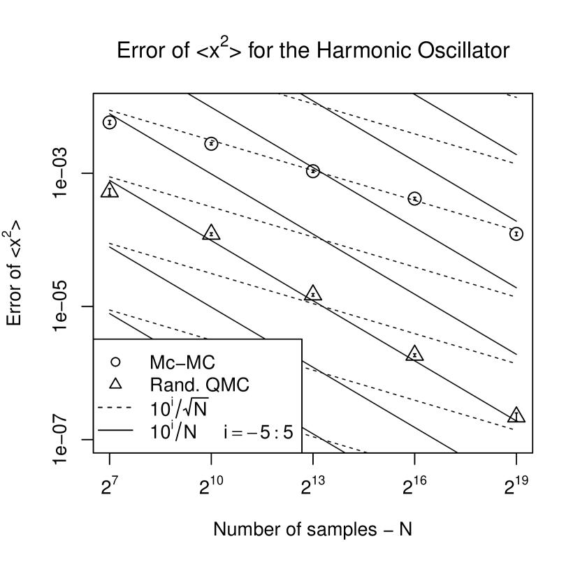
Figure 1: The error of $\langle X^{2}\rangle$ in dependence on the number of samples $N$. The parameters here were chosen as $\lambda=0$ (harmonic oscillator), $d=51$, $M_{0}=0.5$ and $\mu^{2}=2.0$. The error of the error was obtained by repeating the numerical experiment 30 times, see also the text.

Although this example is trivial, it was our first successful application of the QMC approach in a physical lattice model and motivated us to pass on to more complicated models.

8.2 Anharmonic Oscillator

The WUS (reweighting) approach was also used for the problem of the anharmonic oscillator to estimate $\langle X^{4}\rangle$, $\langle X^{2}\rangle$ and the ground state energy of the system ($E_{0}$). With the anharmonic term in action, the probability distribution function (PDF) of the variables $x_{i}$ is of non-Gaussian nature and hence becomes very complicated. This makes it very hard to generate the samples directly from the PDF of the anharmonic oscillator. Instead of this, we consider the WUS method with samples originated from an importance density (see (4.6) in [39]) of Gaussian form, leaving the anharmonic term and a fraction of the harmonic term as part of the functions $f_{1}$ and $f_{2}$ in (18). This change is in part necessary because now we choose $\mu^{2}<0$ in our test cases, and this choice breaks down the positive definiteness of the matrix $C$ from the harmonic oscillator. Thus, we select a new covariance matrix $C^{\star}$ for the Gaussian samples, but we keep the sampling strategy for the $x_{i}$’s essentially unchanged as compared to the harmonic oscillator. The resulting weight functions in 18 are given by

$$f_{1}({\boldsymbol{z}})=O(A^{\star}\Phi^{-1}({\boldsymbol{z}}))f_{2}({\boldsymbol{z}})\;,\quad f_{2}({\boldsymbol{z}})=e^{-\sum_{i}\left(a\left(\frac{\mu^{2}-\mu_{sim}^{2}}{2}\right)(A^{\star}_{i}\Phi^{-1}({\boldsymbol{z}}))^{2}+a\lambda(A^{\star}_{i}\Phi^{-1}({\boldsymbol{z}}))^{4}\right)}\;,$$ (23)

where $A^{\star}_{i}$ stands for the $i$-row of the factorization matrix $A^{\star}$ of $C^{\star}$, and $\mu_{sim}^{2}\geq 0$. As it can be seen from the resulting weight function $f_{2}$, we have chosen the simple strategy of calibrating the diagonal of the new covariance matrix $C^{\star}$ by the use of a parameter $\mu_{sim}^{2}\geq 0$. Besides the requirement of positivity on $C^{\star}$, one is free in the choice of the parameter $\mu_{sim}$. We choose to follow the spirit of importance sampling by tuning $\mu_{sim}$ to a value that reduces the fluctuations of the weights $f_{1}$ and $f_{2}$ as much as possible. The samples based on the tuned parameter $\mu_{sim}$ lead us to observable averages with less variances and therefore smaller errors. Nevertheless, it seems quite difficult to find an optimal criterion for the selection of the functions $f_{1}$, $f_{2}$ and the parameter $\mu_{sim}$ which are leading to the best possible error behavior. At the moment we have to determine these quantities empirically and leave systematic investigations to the future.
Further, it is important to note that the PCA factorization during the generation of the Gaussian samples plays a mayor role for an efficient reduction of the effective dimension (see [33]) of the problem. For the parameters listed below, we estimated the effective dimensions in truncation sense $d_{t}$ of the functions (23) to be close to $20$ (for a $99\%$ variance concentration), for estimating the integrals described in (12) with the dimension of the original system up to $d=1000$. Thus, we observe a drastic reduction of dimensionality.

On the other hand, we found that the effective dimensions in truncation sense of the functions (23) depend very strongly on the parameter $T=da$, i.e. the physical time extent of the system, and seems not sensible to the real dimension $d$. We found that for small $T$-values, say $T<0.2$, the selected parameters $\mu_{sim}$ and PCA lead to a good effective dimension reduction, with $d_{t}$ close to $4$. In this case randomized QMC exhibited an $N^{-1}$ error scaling. The situation changed by increasing the $T$-values. For $T=1.5$ the effective dimensions $d_{t}$ significantly increased to be close to $20$. The exhibited error scaling was $N^{-\alpha}$ with $\alpha\approx 0.75$ for this case. Tests with values of $T\geq 5$ indicate that the simulations become more and more difficult in the sense that one needs more and more samples to achieve the same accuracy of an observable as compared to estimates at $T=1.5$. Thus, in such situations the overlap of the sampling points with the functions $f_{i}$ in 18 seem to be too small to reduce the fluctuations sufficiently. It seems that for this problem there exists some kind of transition range for the observed error scaling using randomized QMC in dependence of the time extent $T$, starting with a convergence rate $N^{-1}$ for $T$-values less than $0.2$ and decreasing to the poor convergence rate $N^{-1/2}$ for $T$-values higher than $5$. However, we are presently exploring a more general approach for selecting a good $T$-dependent matrix $C^{\star}$ (resp. $A^{\star}$ in (23)) in the sampling procedure to improve the situation for larger values of $T$. This question and the relation to the corresponding effective dimension deserves a detailed study, in particular when more realistic models are considered. However, such an investigation, although being very interesting, goes beyond the scope of the present paper.

Nevertheless, for our numerical experiments, the parameters were set to $M_{0}=0.5$, $\lambda=1.0$, $\mu^{2}=-16$. In the two tests the lattice spacing $a$ was adjusted such, that $T$ was kept fixed. The tuned value of $\mu^{2}_{sim}$ generally depends on all physical parameters of the system and in particular on $a$. Thus, we have to adjust also $\mu_{sim}$ when the lattice spacing $a$ is changed. In particular, we set $a=0.015$ and $\mu^{2}_{sim}=0.176$ for $d=100$, whereas for $d=1000$ $a=0.0015$ and $\mu^{2}_{sim}=0.2$ was chosen. The error analysis of $\langle X^{2}\rangle$ and $\langle X^{4}\rangle$ was carried through in the same way as described for the harmonic oscillator test case discussed in the last subsection, 8.1. We show in figure 2 the error of $\langle X^{2}\rangle$ and $E_{0}$ as a function of the number of samples. In addition, we represent by the dashed line in figure 2 a fit to the data for the computed errors using the formula

$$\log\left(\text{ Error }(\langle O\rangle)\right)=\log C+\alpha\log N\;;\quad O=\{x^{2},x^{4},E_{0}\}\;,$$ (24)

with $C$ and $\alpha$ left as free parameters. From this analysis we can obtain a quantitative determination of the exponent of the error scaling. The results for the fit parameters are listed in Table 1.

	$O$	$\alpha$	$\log C$	$\chi^{2}/\text{dof}$
$d=100$	$X^{2}$	-0.763(8)	2.0(1)	7.9 / 6
	$X^{4}$	-0.758(8)	4.0(1)	13.2 / 6
	$E_{0}$	-0.737(9)	4.0(1)	8.3 / 6
$d=1000$	$X^{2}$	-0.758(14)	2.0(2)	5.0 / 4
	$X^{4}$	-0.755(14)	4.0(2)	5.7 / 4
	$E_{0}$	-0.737(13)	4.0(2)	4.0 / 4

Table 1: Shown are the results for fit parameters of the error scaling for the observables considered, i.e. $X^{2}$ , $X^{4}$ and $E_{0}$, where the used fit function takes the form $\mathrm{error}=CN^{\alpha}$, see equation 24. We also provide the $\chi^{2}$ values as well as the number of degrees of freedom in the fit (dof).

As can be inferred from Table 1, in the case of the anharmonic oscillator the error scaling exponent is only $\alpha\approx 0.76$. However, this constitutes still a much improved error scaling compared to a Mc-MC simulation with a corresponding large gain in the number of required samples to reach a desired accuracy. Moreover, the value of $\alpha$ is consistent for all observables considered here and independent from the dimension of the problem $d$, a finding which is clearly encouraging.

We finally mention that the resulting estimates of the ground state energy for $T=1.5$ matches in at least two significant digits with the theoretical value, $E_{0}=3.863$, calculated in [41], namely $\hat{E}_{0}=3.857\pm 0.004$ for $d=100$ and $\hat{E}_{0}=3.862\pm 0.004$ for $d=1000$.

9 Concluding Remarks

In this article we have performed a first application of QMC methods to Euclidean lattice models. The goal was to see, whether QMC algorithms provide also in the case of non-Gaussian systems an improved error scaling behavior with respect to Markov-chain Monte Carlo methods. As a prototype system, we have considered the quantum mechanical oscillator discretized on a Euclidean time lattice, both in its harmonic (Gaussian) form as well as adding a non-Gaussian quartic term (anharmonic oscillator). For the harmonic oscillator we found a large-$N$ ($N$ being the number of sample points) immproved error behavior, i.e. $\sim N^{-1}$ for (randomized) QMC and $\sim N^{-1/2}$ for Mc-MC.

The main result of our investigation is that also for the anharmonic oscillator, which is a non-Gaussian problem, the QMC approach leads to a significant improvement of the error scaling $N^{\alpha}$ with $\alpha\approx-0.76$, see Table 1 for the exact values of $\alpha$ for different observables and different physical situations.

Further, we found that the accessible range of $T=1.5$ values gives already estimates of the ground state energy, compatible (within errors) with the theoretical prediction (valid in the limit $T\rightarrow\infty$ and $a\rightarrow 0$). For the case that the improved error scaling and the mild dependence on the lattice spacing $a$ found here will also be present in more elaborate models, QMC methods have the potential to become very valuable in the future. On the other hand we observed that the applicability of the WUS (reweighting) approach seems to be limited by the physical time extent $T=da$ of the system. For values of $T\leq 1.5$ the error falls below the percent level within the investigated number of samples. For increasing values of $T$ the error is continuously growing and at $T=5$ we can only obtain a relative error of $\approx 15\%$ for $2^{19}$ samples. For larger $T$ values we expect the error to become even larger leading eventually for very large $T$ to a situation where a meaningful evaluation of the considered quantities is not possible anymore. This behavior and the relation to the effective dimension of the problem clearly needs an understanding and a dedicated investigation in the future, in particular, when more realistic models are considered.

It is clear that the here considered quantum mechanical systems are rather simple models and still a long way has to be gone, if generic quantum field theories, especially gauge theories are to be studied. Nevertheless, it is very reassuring that we find an improved error scaling behavior in the case of a quartic potential and hence a non-Gaussian system. This promising result is certainly a strong motivation for studying further QMC methods in lattice field theories and statistical mechanics.

10 Appendix: C++ programme for the QMC simulation of the (an)harmonic oscillator

We provide a C++ programme for the QMC simulation of the (an)harmonic oscillator at the following URL http://arxiv.org/format/1302.6419v3 (“Source”). In the following we give a short description for the usage of the programme. The programme implements the suggested algorithm for the evaluation of the path integral of the harmonic and anharmonic oscillator in the QMC approach, except that the present implementation applies random digital shifts instead of random scramblings to generate different sobol sequences. Eventually, both methods should lead to very similar results.
Copyright information may be obtained from the file “README” in the package. The package is equipped with a standard “Makefile” and a cmake input file “CMakeList.txt”.

10.1 Prerequisites

The only external dependency is the FFTW library version 3 which can be obtained from http://www.fftw.org. The FFTW library offers an efficient implementation of the Hartley transform.
If the library is installed in a non-standard path of your PC, you can adjust the variable “FFTWDIR” in the very beginning of the make file or via the environment variable “FFTWDIR” when using “CMakeLists.txt”.

10.2 Building

Simply run ’make’ when using “Makefile” or use ’ccmake <path to package source>’ in an empty directory followed by a ’make’.

10.3 Parameters

Having built the executable ’qmc_quartic_reweight’ you can run the programme, preferably in a new empty directory, and may pass the following parameters:

Parameter	Meaning
-N <Integer>	number of dimensions
-k <Integer>	number of samples per estimation
-c <Integer>	number of configurations written out to a file
-S <Integer>	max. time separation for correlator
-a <Float>	lattice spacing $a$
-M <Float>	particle mass $M_{0}$
-m <Float>	$\mu^{2}_{sim}$
-u <Float>	$\mu^{2}$
-l <Float>	$\lambda$
-Q <Path to file>	file containing directions numbers

.

Files with direction numbers can be obtained from Frances Kuo’s page http://web.maths.unsw.edu.au/~fkuo/sobol/index.html. The programme produces 10 estimations, each with the given number of samples. Output is written to files of the form
<prefix>_s1_N<# dimensions>_a<a>_M0<M0>_musq<mu^2_sim>_l<lambda>_J0.000000.csv. The result of each estimation is stored in the file with the prefix “obs_macro”. The first column contains the estimated value of $\langle x^{2}\rangle$ and the second column contains $\langle x^{4}\rangle$. Successive runs of the programme with the same parameters will append 10 more estimates. Correspondingly, 30 runs should suffice to produce the statistics we used in this work.

References

- [1] Christof Gattringer and Christian B. Lang. Quantum chromodynamics on the lattice. Lect.Notes Phys., 788:1–211, 2010.
- [2] I. Montvay and G. Münster. Quantum fields on a lattice. Cambridge Monographs on Mathematical Physics. Cambridge University Press, 1994.
- [3] Zoltan Fodor and Christian Hoelbling. Light Hadron Masses from Lattice QCD. Rev.Mod.Phys., 84:449, 2012.
- [4] John Bulava, Philipp Gerhold, Karl Jansen, Jim Kallarackal, Bastian Knippschild, et al. Higgs-Yukawa model in chirally-invariant lattice field theory. Adv. High Energy Phys., 2013:875612, 2013.
- [5] Pierre L’Ecuyer and Christiane Lemieux. Recent advances in randomized quasi-monte carlo methods. In Moshe Dror, Pierre L’Ecuyer, and Ferenc Szidarovszky, editors, Modeling Uncertainty, volume 46 of International Series in Operations Research & Management Science, pages 419–474. Springer US, 2005.
- [6] F. Kuo, Ch. Schwab, and I. Sloan. Quasi-monte carlo methods for high-dimensional integration: the standard (weighted hilbert space) setting and beyond. ANZIAM Journal, 53(0), 2012.
- [7] Paul Glasserman. Monte Carlo methods in financial engineering, volume 53 of Applications of Mathematics (New York). Springer-Verlag, New York, 2004. Stochastic Modelling and Applied Probability.
- [8] P. Jäckel. Monte Carlo Methods in Finance. The Wiley Finance Series. Wiley, 2002.
- [9] M. Creutz and B. A. Freedman. A statistical approach to quantum mechanics. Ann. Phys., 132:427–462, 1981. available online in Michael Creutz’s publication list under http://thy.phy.bnl.gov/~creutz/mypubs/pubs.html, visited June 17 2013.
- [10] W. Bietenholz, U. Gerber, M. Pepe, and U.-J. Wiese. Topological Lattice Actions. JHEP, 1012:020, 2010.
- [11] K. Jansen, H. Leovey, A. Nube, A. Griewank, and M. Mueller-Preussker. A first look at quasi-Monte Carlo for lattice field theory problems. 2012. available online under http://arxiv.org/pdf/1211.4388.pdf.
- [12] M. J. D. Powell and J. Swann. Weighted uniform sampling – a monte carlo technique for reducing variance. J.Inst.Maths Applics, 2:228–236, 1966.
- [13] Makoto Matsumoto and Takuji Nishimura. Mersenne twister: a 623-dimensionally equidistributed uniform pseudo-random number generator. ACM Trans. Model. Comput. Simul., 8(1):3–30, January 1998.
- [14] Erich Novak and Henryk Woźniakowski. Tractability of multivariate problems. Volume II: Standard information for functionals, volume 12 of EMS Tracts in Mathematics. European Mathematical Society (EMS), Zürich, 2010.
- [15] Josef Dick and Friedrich Pillichshammer. Digital Nets and Sequences: Discrepancy Theory and Quasi-Monte Carlo Integration. Cambridge University Press, New York, NY, USA, 2010.
- [16] Russel E. Caflisch. Monte carlo and quasi-monte carlo methods. Acta Numerica, 7:1–49, 0 1998.
- [17] Fred J. Hickernell. A generalized discrepancy and quadrature error bound. Math. Comp, 67:299–322, 1998.
- [18] Ian H. Sloan and Henryk Wozniakowski. When are quasi-monte carlo algorithms efficient for high dimensional integrals? J. Complexity, 14:1–33, 1997.
- [19] F. Y. Kuo. Component-by-component constructions achieve the optimal rate of convergence for multivariate integration in weighted Korobov and Sobolev spaces. J. Complexity, 19(3):301–320, 2003.
- [20] Xiaoqun Wang. Strong tractability of multivariate integration using quasi-monte carlo algorithms. Math. Comp., 72(242):823–838, April 2003.
- [21] A. Griewank, L. Lehmann, H. Leovey, and M. Zilberman. Automatic evaluations of cross-derivatives. to appear in Math. Comp., 2012.
- [22] Harald Niederreiter. Random number generation and quasi-Monte Carlo methods, volume 63 of CBMS-NSF Regional Conference Series in Applied Mathematics. Society for Industrial and Applied Mathematics (SIAM), Philadelphia, PA, 1992.
- [23] I. M. Sobol’. The distribution of points in a cube and the approximate evaluation of integrals. U.S.S.R. Comput. Math. and Math. Phys., 7(4):86–112, 1967.
- [24] Paul Bratley and Bennett L. Fox. Algorithm 659: Implementing sobol’s quasirandom sequence generator. ACM Trans. Math. Softw., 14(1):88–100, 1988.
- [25] Stephen Joe and Frances Y. Kuo. Remark on algorithm 659: Implementing sobol’s quasirandom sequence generator. ACM Trans. Math. Softw., 29(1):49–57, March 2003.
- [26] Stephen Joe and Frances Y. Kuo. Constructing sobol sequences with better two-dimensional projections. SIAM J. Sci. Comput., 30(5):2635–2654, August 2008.
- [27] Ilya M. Sobol’, Danil Asotsky, Alexander Kreinin, and Sergei Kucherenko. Construction and comparison of high-dimensional sobol’ generators. Wilmott, 2011(56):64–79, 2011.
- [28] A. B. Owen. Randomly permuted -nets and -sequences. In H. Niederreiter and P. J.-S. Shiue, editors, Monte Carlo and Quasi-Monte Carlo Methods in Scientific Computing, volume 106 of Lecture Notes in Statistics, pages 299–317. Springer-Verlag, 1995.
- [29] Art B. Owen. Monte carlo variance of scrambled net quadrature. SIAM J. Numer. Anal., 34(5):1884–1910, October 1997.
- [30] Art B. Owen. Local antithetic sampling with scrambled nets. Ann. Statist., 36:2319–2343, 2008.
- [31] J. Matousěk. On the -discrepancy for anchored boxes. Journal of Complexity, 14:527–556, 1998.
- [32] Shu Tezuka and Henri Faure. I-binomial scrambling of digital nets and sequences. Journal of Complexity, 19(6):744 – 757, 2003.
- [33] R. E. Caflisch, W. Morokoff, and A. Owen. Valuation of mortgage-backed securities using Brownian bridges to reduce effective dimension. The Journal of Computational Finance, 1(1):27–46, 1997.
- [34] I. M. Sobol’. Global sensitivity indices for nonlinear mathematical models and their Monte Carlo estimates. Math. Comput. Simulation, 55(1-3):271–280, 2001. The Second IMACS Seminar on Monte Carlo Methods (Varna, 1999).
- [35] Xiaoqun Wang and Kai-Tai Fang. The effective dimension and quasi-Monte Carlo integration. J. Complexity, 19(2):101–124, 2003.
- [36] X. Wang and I. Sloan. Why are high-dimensional finance problems often of low effective dimension? SIAM Journal on Scientific Computing, 27(1):159–183, 2005.
- [37] I.M. Sobol’ and S. Kucherenko. Derivative based global sensitivity measures and their link with global sensitivity indices. Math. Comput. Simul., 79(10):3009–3017, 2009.
- [38] Andreas Griewank and Andrea Walther. Evaluating derivatives. Society for Industrial and Applied Mathematics (SIAM), Philadelphia, PA, second edition, 2008. Principles and techniques of algorithmic differentiation.
- [39] Jerome Spanier and Earl H. Maize. Quasi-random methods for estimating integrals using relatively small samples. SIAM Rev., 36(1):18–44, March 1994.
- [40] Russel E. Caflisch and Bradley Moskowitz. Modified monte carlo methods using quasi-random sequences. In Lecture Notes in Statistics 106, pages 1–16. Springer-Verlag, 1995.
- [41] Richard Blankenbecler, Thomas A. DeGrand, and R.L. Sugar. Moment Method for Eigenvalues and Expectation Values. Phys.Rev., D21:1055, 1980.
- [42] Frances Y. Kuo, Ian H. Sloan, Grzegorz W. Wasilkowski, and Henryk Woźniakowski. On decompositions of multivariate functions. Math. Comput., 79(270):953–966, 2010.
- [43] I.G. Graham, F.Y. Kuo, D. Nuyens, R. Scheichl, and I.H. Sloan. Quasi-monte carlo methods for elliptic pdes with random coefficients and applications. Journal of Computational Physics, 230(10):3668 – 3694, 2011.