Convex vs nonconvex approaches for sparse estimation:
GLasso, Multiple Kernel Learning and Hyperparameter GLasso

Abstract

The popular Lasso approach for sparse estimation can be derived via marginalization of a joint density associated with a particular stochastic model. A different marginalization of the same probabilistic model leads to a different non-convex estimator where hyperparameters are optimized. Extending these arguments to problems where groups of variables have to be estimated, we study a computational scheme for sparse estimation that differs from the Group Lasso. Although the underlying optimization problem defining this estimator is non-convex, an initialization strategy based on a univariate Bayesian forward selection scheme is presented. This also allows us to define an effective non-convex estimator where only one scalar variable is involved in the optimization process. Theoretical arguments, independent of the correctness of the priors entering the sparse model, are included to clarify the advantages of this non-convex technique in comparison with other convex estimators. Numerical experiments are also used to compare the performance of these approaches.

Keywords: Lasso; Group Lasso; Multiple Kernel Learning; Bayesian regularization; marginal likelihood

1 Introduction

We consider sparse estimation in a linear regression model where the explanatory factors $\theta\in{\mathbb{R}}^{m}$ are naturally grouped so that $\theta$ is partitioned as $\theta=[{\theta^{(1)}}^{\top}\quad{\theta^{(2)}}^{\top}\quad\ldots\quad{\theta^{(p)}}^{\top}]^{\top}$. In this setting we assume that $\theta$ is group (or block) sparse in the sense that many of the constituent vectors $\theta^{(i)}$ are zero or have a negligible influence on the output $y\in{\mathbb{R}}^{n}$. In addition, we assume that the number of unknowns $m$ is large, possibly larger than the size of the available data $n$. Interest in general sparsity estimation and optimization has attracted the interest of many researchers in statistics, machine learning, and signal processing with numerous applications in feature selection, compressed sensing, and selective shrinkage (Hastie and Tibshirani, 1990; Tibshirani, 1996; Donoho, 2006; Candes and Tao, 2007). The motivation for our study of the group sparsity problem comes from the “dynamic Bayesian network” scenario identification problem as discussed in (Chiuso and Pillonetto, 2011, 2010b, 2010a). In a dynamic network scenario the “explanatory variables” are often the past histories of different input signals with the “groups” $\theta^{(i)}$ representing the impulse responses describing the relationship between the $i$-th input and the output $y$. This application informs our view of the group sparsity problem as well as our measures of success for a particular estimation procedure.

Several approaches have been put forward in the literature for joint estimation and variable selection problems. We cite the well known Lasso (Tibshirani, 1996), Least Angle Regression (LAR) (Efron et al., 2004), their “group” versions Group Lasso (GLasso) and Group Least Angle Regression (GLAR) (Yuan and Lin, 2006), Multiple Kernel Learning (MKL) (Bach et al., 2004; Evgeniou et al., 2005; Pillonetto et al., 2010). Methods based on hierarchical Bayesian models have also been considered such as Automatic Relevance Determination (ARD) (Mackay, 1994), the Relevance Vector Machine (RVM) (Tipping, 2001), and the exponential hyperprior in (Chiuso and Pillonetto, 2010b, 2011). The Bayesian approach considered in (Chiuso and Pillonetto, 2010b, 2011) and further developed in this paper is intimately related to (Mackay, 1994; Tipping, 2001); in fact, the exponential hyperprior algorithm in (Chiuso and Pillonetto, 2010b, 2011) is a penalized version of ARD. A variational approach based on the golden standard spike and slab prior, also called two-groups prior (Efron, 2008), has been also recently proposed in (Titsias and L zaro-Gredilla, 2011).

An interesting series of papers (Wipf and Rao, 2007; Wipf and Nagarajan, 2007; Wipf et al., 2011) provide a nice link between penalized regression problems like Lasso, also called type-I methods, and Bayesian methods (like RVM (Tipping, 2001) and ARD (Mackay, 1994)) with hierarchical hyperpriors where the “hyperparameters” are estimated via maximizing the marginal likelihood and then inserted in the Bayesian model following the Empirical Bayes paradigm (Maritz and Lwin, 1989); these latter methods are also known as type-II methods (Berger, 1985). Note that this Empirical Bayes paradigm has also been recently used in the context of System Identification (Pillonetto and De Nicolao, 2010; Pillonetto et al., 2011; Chen et al., 2011).

In (Wipf and Nagarajan, 2007; Wipf et al., 2011) it is argued that type-II methods have advantages over type-I methods; some of these advantages are related to the fact that, under suitable assumptions, the former can be written in the form of type-I with the addition of a non-separable penalty term (a function $g(x_{1},..,x_{n})$ is non-separable if it cannot be written as $g(x_{1},..,x_{n})=\sum_{i=1}^{n}h(x_{i})$). The analysis in (Wipf et al., 2011) also suggests that in the low noise regime the type-II approach results in a “tighter” approximation to the $\ell_{0}$ norm. This is supported by experimental evidence showing that these Bayesian approaches perform well in practice. Our experience is that the approach based on the marginal likelihood is particularly robust w.r.t. noise regardless of the “correctness” of the Bayesian prior.

Motivated by the nice performance of the exponential hyperprior approach introduced in the dynamic network identification scenario (Chiuso and Pillonetto, 2010b, 2011), we provide some new insights clarifying the above issues. The main contributions are as follows:

1. in the first part of the paper we discuss the relation among Lasso (and GLasso), the Exponential Hyperprior (HGLasso algorithm hereafter, for reasons which will become clear later on) and MKL by putting all these methods in a common Bayesian framework (similar to that discussed in (Park and Casella, 2008)). Lasso/GLasso and MKL boil down to convex optimization problems, leading to identical estimators, while HGLasso does not.

2. All these methods are then compared in terms of optimality (KKT) conditions and tradeoffs between sparsity and shrinkage are studied illustrating the advantages of HGLasso over GLasso (or, equivalently, MKL). Also the properties of Empirical Bayes estimators which form the basis of our computational scheme are studied in terms of their Mean Square Error properties; this is first established in the simplest case of orthogonal regressors and then extended to more general cases allowing for the regressors to be realizations from, possibly correlated, stochastic processes. This, of course, is of paramount importance for the system identification scenario studied in (Chiuso and Pillonetto, 2010b, 2011).

   Our analysis avoids assumptions on the correctness of the priors entering the stochastic model and clarifies why HGLasso is likely to provide more sparse and accurate estimates in comparison with the other two convex estimators. As a byproduct, our study also clarifies the asymptotic properties of ARD.

3. Since HGLasso requires solving non-convex, and possibly high-dimensional, optimization problems we introduce a version of our computational scheme which can be used as an initialization for the full non-convex search requiring optimization with respect to only one scalar variable representing a common scale factor for the hyperparameters. Such Bayesian schemes with a hyperprior having a common scale factor, or more generally group problems in which each group is described by one hyperparameter, can be seen as instances of “Stein estimators” (James and Stein, 1961; Efron and Morris, 1973; Stein, 1981) and have close connections to the non-negative garrote estimator (Breiman, 1995). The initialization we propose is based on a selection scheme which departs from classical Bayesian variable selection algorithms (George and McCulloch, 1993; George and Foster, 2000; Scott and Berger, 2010). These latter methods are based on the introduction of binary (Bernoulli) latent variables. Instead our strategy involves a “forward selection” type of procedure which may be seen as an instance of the “screening” type of approach for variable selection discussed in (Wang, 2009); note however that while classical forward selection procedures work in “parameter space” our forward selection is performed in hyperparameter space through the marginal posterior (i.e. once the parameters $\theta$ are integrated out); in the asymptotic regime this procedure is equivalent to performing forward selection using BIC as a criterion. This “finite data” Bayesian flavor seems to be a key feature which makes the procedure remarkably robust as the experimental results confirm. Note that backward and forward-backward versions of this procedure have also been tested with no notable differences.

4. Extensive numerical experiments involving artificial and real data are included which confirm the superiority of HGLasso.
   

The paper is organized as follows. In Section 2 we introduce the Lasso approach in a Bayesian framework, as well as another estimator, namely HLasso, that requires the optimization of hyperparameters. Section 3 extends the arguments to a group version of the sparse estimation problem introducing GLasso and the group version of HLasso which we call HGLasso. In Section 4 the relationship between HGLasso and MKL is discussed, reviewing the equivalence between GLasso and MKL. Section 5 clarifies the advantages of HGLasso over GLasso and MKL on a simple example. In Section 6 the Mean Squared Error properties of the Empirical Bayes estimators are studied, including their asymptotic behavior. In Section 7 we discuss the implementation of our computational scheme, also deriving a version of HGLasso that requires the optimization of an objective only with respect to one scalar variable. Section 8 reports numerical experiments involving artificial and real data, also comparing the new approach with the adaptive Lasso described in (Zou, 2006). Some conclusions end the paper.

2 Lasso and HLasso

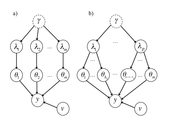
Figure 1: Bayesian networks describing the stochastic model for sparse estimation (a) and group sparse estimation (b)

Let $\theta=[\theta_{1}\quad\theta_{2}\ldots\theta_{m}]^{\top}$ be an unknown parameter vector while $y\in{\mathbb{R}}^{n}$ denotes the vector containing some noisy data. In particular, our measurements model is

$$y=G\theta+v$$ (1)

where $G\in{\mathbb{R}}^{n\times m}$ and $v$ is the vector whose components are white noise of known variance $\sigma^{2}$.

2.1 The Lasso

Under the assumption that $\theta$ is sparse, i.e. many of its components are equal to zero or have a negligible influence on $y$, a popular approach to reconstruct the parameter vector is the Lasso (Tibshirani, 1996). The Lasso estimate of $\theta$ is given by

$$\hat{\theta}_{L}=\arg\min_{\theta}\frac{(y-G\theta)^{\top}(y-G\theta)}{2\sigma^{2}}+\gamma_{L}\sum_{i=1}^{m}|\theta_{i}|$$ (2)

where $\gamma_{L}\in{\mathbb{R}}_{+}$ is the regularization parameter. A key feature of the Lasso is that the estimate $\hat{\theta}_{L}$ is the solution to a convex optimization problem.

As in (Park and Casella, 2008), we describe a derivation of the Lasso through the marginalization of a suitable probability density function. This hierarchical representation is useful for establishing a connection with the variety of estimators considered in this paper. The Bayesian model we consider is depicted in Fig. 1(a). Nodes and arrows are either dotted or solid depending on being representative of, respectively, deterministic or stochastic quantities/relationships. Here, $\lambda$ denotes a vector whose components $\{\lambda_{i}\}_{i=1}^{m}$ are independent and identically distributed exponential random variables with probability density

$$p_{\gamma}(\lambda_{i})=\gamma e^{-\gamma\lambda_{i}}\chi(\lambda_{i}),$$ (3)

where $\gamma$ is a positive scalar while $\chi(t)=1$ if $t\geq 0$, 0 otherwise. In addition

$$\theta_{i}|\lambda_{i}\sim{\mathcal{N}}(0,\lambda_{i})\qquad\mbox{and}\qquad v\sim{\mathcal{N}}(0,\sigma^{2}I_{n}),$$ (4)

where ${\mathcal{N}}(\mu,\Sigma)$ is the Gaussian density of mean $\mu$ and covariance $\Sigma$ while $I_{n}$ is the $n\times n$ identity matrix. We have the following result from Section 2 in (Park and Casella, 2008).

Theorem 1

Given the Bayesian network in Fig. 1(a), let

$$\hat{\theta}=\arg\max_{\theta\in{\mathbb{R}}^{m}}\int_{{\mathbb{R}}_{+}^{m}}p(\theta,\lambda|y)d\lambda,$$ (5)

Then $\hat{\theta}=\hat{\theta}_{L}$ provided that $\gamma_{L}=\sqrt{2\gamma}$.

2.2 The HLasso

Theorem 1 inspires the definition of an estimator obtained by marginalizing with respect to $\theta$ instead of $\lambda$ and then maximizing the resulting marginal density $p(\lambda|y)$ with respect to $\lambda$ obtaining an estimate $\hat{\lambda}$ for $\lambda$. Having $\hat{\lambda}$, we use an empirical Bayes approach and set $\hat{\theta}_{HL}:={\mathbb{E}}[\theta|y,\hat{\lambda}]$ (the minimum variance estimate of $\theta$ given $y$ and $\lambda=\hat{\lambda}$). We call $\hat{\theta}_{HL}$ the Hyperparameter Lasso (HLasso). This estimator is given in the next theorem which uses the fact that $\theta$ conditional on $\lambda$ is Gaussian, so that the marginal density of $\lambda$ is available in closed form. The proof flows from the following observations:

$$p(\theta,\lambda|y) \propto |\Lambda|^{-1/2}\exp[-\frac{1}{2}y^{\top}\Sigma_{y}(\lambda)^{-1}y]$$

$$\bullet\exp[-\frac{1}{2}(\theta-\theta_{HL}(\lambda))^{\top}(\Lambda^{-1}+\sigma^{-2}G^{\top}G)(\theta-\theta_{HL}(\lambda))]\exp[-\gamma\mathbf{1}^{\top}\lambda],$$

where

$$\Lambda=\mbox{diag}(\lambda),\qquad\Sigma_{y}(\lambda):=(\sigma^{2}I+G\Lambda G^{\top}),$$ (7)

and

$$\theta_{HL}(\lambda):={\mathbb{E}}[\theta|y,{\lambda}]=(\sigma^{2}\Lambda^{-1}+G^{\top}G)^{-1}G^{\top}y=\Lambda G^{\top}\Sigma_{y}(\lambda)^{-1}y$$ (8)

Notice that the equivalence of the two expressions for the $\theta_{HL}(\lambda)$ follows from the matrix inversion formula

$$\Sigma_{y}(\lambda)^{-1}=\sigma^{-2}\left[I-G(\sigma^{2}\Lambda^{-1}+G^{T}G)^{-1}G^{\top}\right].$$ (9)

Also note that (8) assures us that $\theta_{HL}(\lambda)$ well defined even when some of the components of $\lambda$ are zero. The matrix $\Sigma_{y}(\lambda)$ plays a fundamental role in much of the analysis of this paper. The Law of Iterated Expectation tells us that $\Sigma_{y}(\lambda)$ is simply the second moment of $y$ given $\lambda$, indeed,

$${\mathbb{E}}[yy^{\top}\,|\,\lambda] = {\mathbb{E}}[{\mathbb{E}}[yy^{\top}\,|\,\theta]\,|\,\lambda]$$ (10)

$$= {\mathbb{E}}[\mbox{Var}[y\,|\,\theta]+{\mathbb{E}}[y\,|\,\theta]{\mathbb{E}}[y\,|\,\theta]^{\top}\,|\,\lambda]$$

$$= {\mathbb{E}}[\sigma^{2}I+G\theta\theta^{\top}G^{\top}\,|\,\lambda]$$

$$= \sigma^{2}I+G{\mathbb{E}}[\theta\theta^{\top}\,|\,\lambda]G^{\top}$$

$$= \Sigma_{y}(\lambda).$$

Theorem 2

Given the Bayesian network in Fig. 1(a), let

$$\hat{\lambda}=\arg\max_{\lambda\in{\mathbb{R}}_{+}^{m}}\int_{{\mathbb{R}}^{m}}p(\theta,\lambda|y)d\theta.$$ (11)

Then

$$\hat{\lambda}=\arg\min_{\lambda\in{\mathbb{R}}_{+}^{m}}\frac{1}{2}\log\det(\Sigma_{y}(\lambda))+\frac{1}{2}y^{\top}(\Sigma_{y}(\lambda))^{-1}y+\gamma\sum_{i=1}^{m}\lambda_{i},$$ (12)

and, given $\lambda=\hat{\lambda}$, the HLasso estimate of $\theta$ is given by

$$\hat{\theta}_{HL}:={\mathbb{E}}[\theta|y,\hat{\lambda}].$$ (13)

$\blacksquare$

The objective in (11) depends on $m$ variables as in the Lasso case, however the optimization problem is no-longer convex since the function $\log\det(\Sigma_{y}(\lambda))$ is a concave function of $\lambda$ as it is the composition of the concave function $\log\det(\Sigma)$ and the affine function $\Sigma_{y}(\lambda)$.

It is worth observing that the estimator obtained from (11) and (13) is a form of “Sparse Bayesian Learning” having close resemblance with ARD (Mackay, 1994) and RVM (Tipping, 2001), see also (Wipf and Nagarajan, 2007). In fact ARD is obtained by setting $\gamma$ in (12) to zero while the Gamma prior used in RVM (see eq. (6) in (Tipping, 2001)) seems to play a symmetric role, favoring large values of $\lambda_{i}$’s. Note that the Gamma prior in equation (6) of (Tipping, 2001) becomes flat as $a\rightarrow$ and $b\rightarrow 0$, similarly to (3) as $\gamma\rightarrow 0$. A similar discussion applies also to the Group version of this estimator to be introduced in Section 3.2.

In Sections 5 and 6 we show that the parameter $\gamma$ plays a fundamental role in enforcing sparsity. In addition, we establish an interesting interpretation in terms of the Mean Squared Error properties of the resulting estimators as $\gamma\rightarrow 0$. Note also that $\gamma$ plays a fundamental role in model selection consistency (see Remark 11).

3 GLasso and HGLasso

We now consider a situation where the explanatory factors $G$ used to predict $y$ are grouped. Think of $\theta$ as being partitioned into $p$ sub-vectors $\theta^{(i)}$, $i=1,\dots,p$, so that

$$\theta=[{\theta^{(1)}}^{\top}\quad{\theta^{(2)}}^{\top}\quad\ldots\quad{\theta^{(p)}}^{\top}]^{\top}.$$ (14)

For $i=1,\dots,p$, assume that the sub-vector $\theta^{(i)}$ has dimension $k_{i}$ so that $m=\sum_{i=1}^{p}k_{i}$. Next, conformally partition the matrix $G=[G^{(1)},\dots,G^{(p)}]$ to obtain the measurement model

$$y=G\theta+v=\sum_{i=1}^{p}G^{(i)}\theta^{(i)}+v.$$ (15)

In what follows, we assume that $\theta$ is block sparse in the sense that many of the blocks $\theta^{(i)}$ are null, i.e. with all of their components equal to zero, or have a negligible effect on $y$.

3.1 The GLasso

A leading approach for the block sparsity problem is the Group Lasso (GLasso) (Yuan and Lin, 2006). The Group Lasso determines the estimate of $\theta$ as

$$\hat{\theta}_{GL}=\arg\min_{\theta\in{\mathbb{R}}^{m}}\frac{(y-G\theta)^{\top}(y-G\theta)}{2\sigma^{2}}+\gamma_{GL}\sum_{i=1}^{p}\|\theta^{(i)}\|\,,$$ (16)

where $\|\cdot\|$ denotes the classical Euclidean norm. Notice that the representation (16) assumes that the $\theta^{(i)}$ are i.i.d. with

$$p(\theta^{(i)}\,\,|\gamma_{GL})\propto\mathrm{exp}\left[-\gamma_{GL}\|\theta^{(i)}\|\right].$$

It is easy to see that, as in the Lasso case, the objective is convex.

3.2 The HGLasso

An alternative approach to the block sparsity problem is discussed in (Chiuso and Pillonetto, 2010b). This approach relies on the group version of the model in Fig. 1(a) illustrated in Fig. 1(b). In the network, $\lambda$ is now a $p$-dimensional vector with $i-th$ component given by $\lambda_{i}\in{\mathbb{R}}_{+}$. In addition, conditional on $\lambda$, each block $\theta^{(i)}$ of the vector $\theta$ is zero-mean Gaussian with covariance $\lambda_{i}I_{k_{i}}$, $i=1,..,p$, i.e.

$$\theta^{(i)}|\lambda_{i}\sim N(0,{\lambda}_{i}I_{k_{i}}).$$ (17)

As for the HLasso, the proposed estimator first optimizes the marginal density of $\lambda$, and then again using an empirical Bayes approach, the minimum variance estimate of $\theta$ is computed with $\lambda$ taken as known and set to its estimate. We call this scheme Hyperparameter Group Lasso (HGLasso). It is described in the following theorem.

Theorem 3

Consider the Bayesian network in Fig. 1 (b) with measurement model given by (15), (17), and (3), and define

$$\hat{\lambda}=\arg\max_{\lambda\in{\mathbb{R}}_{+}^{p}}\int_{{\mathbb{R}}^{m}}p(\theta,\lambda|y)d\theta.$$ (18)

Then, $\hat{\lambda}$ is given by

$$\arg\min_{{\lambda}\in{\mathbb{R}}_{+}^{p}}\frac{1}{2}\log\det(\Sigma_{y}(\lambda))+\frac{1}{2}y^{\top}\Sigma_{y}^{-1}(\lambda)y+\gamma\sum_{i=1}^{p}{\lambda}_{i},$$ (19)

where

$$\Sigma_{y}(\lambda):=G\Lambda G^{\top}+\sigma^{2}I,\qquad\Lambda:=\mbox{blockdiag}(\{{\lambda}_{i}I_{k_{i}}\}).$$ (20)

In addition, the HGLasso estimate of $\theta$, denoted $\hat{\theta}_{HGL}$, is given by setting $\lambda=\hat{\lambda}$ in the function

$${\theta}_{HGL}(\lambda):={\mathbb{E}}[\theta|y,\lambda]=\Lambda G^{\top}(\Sigma_{y}({\lambda}))^{-1}y.$$ (21)

$\blacksquare$

The derivation of this estimate is virtually identical to the derivation of the estimate given in Theorem 2. For this reason, we slightly abuse our notation by not introducing a new notation for the key affine matrix mapping $\Sigma_{y}(\lambda)$. Just as in the HLasso case, the objective in (19) is not convex in $\lambda$. However, now the optimization is performed in the lower dimensional space ${\mathbb{R}}^{p}$, rather than in ${\mathbb{R}}^{m}$ where the GLasso objective is optimized.

Let the vector $\mu$ denote the dual vector for the constraint $\lambda\geq 0$. Then the Lagrangian for the problem (19) is given by

$$\begin{array}[]{lll}L(\lambda,\mu):=\frac{1}{2}\log\det(\Sigma_{y}(\lambda))+\frac{1}{2}y^{\top}\Sigma_{y}(\lambda)^{-1}y+\gamma{\bf 1}^{\top}\lambda-\mu^{\top}\lambda.\end{array}$$ (22)

Using the fact that

$$\partial_{\lambda_{i}}L(\lambda,\mu) = \frac{1}{2}\mbox{tr}\left(G^{(i)\top}\Sigma_{y}(\lambda)^{-1}G^{(i)}\right)$$

$$- \frac{1}{2}y^{\top}\Sigma_{y}(\lambda)^{-1}G^{(i)}G^{(i)\top}\Sigma_{y}(\lambda)^{-1}y+\gamma\ -\mu_{i},$$

we obtain the following KKT conditions for (19).

Proposition 4

The necessary conditions for $\lambda$ to be a solution of (19) are

$$\begin{array}[]{l}\Sigma_{y}=\sigma^{2}I+\sum_{i=1}^{p}\lambda_{i}G^{(i)}G^{(i)\top}\\ W\Sigma_{y}=I\\ \mbox{tr}\left(G^{(i)\top}WG^{(i)}\right)-\|G^{(i)\top}Wy\|_{2}^{2}+2\gamma-2\mu_{i}=0,\quad i=1,\dots,p\\ \mu_{i}\lambda_{i}=0,\quad i=1,\dots,p\\ 0\leq\mu,\ \lambda\mbox{ and }0\preceq W,\Sigma_{y}.\end{array}$$ (23)

It is interesting to observe that, by (10), one has

$${\mathbb{E}}\left[\theta_{HGL}(\lambda)\theta_{HGL}(\lambda)^{\top}\,|\,\lambda\right]=\Lambda G^{\top}\Sigma_{y}({\lambda})^{-1}{\mathbb{E}}[yy^{\top}\,|\,\lambda]\Sigma_{y}({\lambda})^{-1}G\Lambda=\Lambda G^{\top}\Sigma_{y}({\lambda})^{-1}G\Lambda,$$

and so

$${\mathbb{E}}\left[\left.\theta_{HGL}^{(i)}(\lambda)\left(\theta_{HGL}^{(i)}(\lambda)\right)^{\top}\,\right|\,\lambda\right]=\lambda_{i}^{2}\left(G^{(i)\top}WG^{(i)}\right),\quad i=1,\dots,p.$$ (24)

In addition,

$$\|\theta_{HGL}^{(i)}(\lambda)\|^{2}=\lambda_{i}^{2}\|G^{(i)\top}Wy\|_{2}^{2},\quad i=1,\dots,p.$$

Equation (23) indicates that when tuning $\lambda$ there should be a link between the “norm” of the actual estimator $\|\hat{\theta}^{(i)}(\lambda)\|^{2}$ to its a priori second moments (24). In particular, when no regularization is imposed on $\lambda$ (i.e. $\gamma=0$) and the nonnegativity constraint is not active, i.e. $\mu_{i}=0$, one finds that the optimal value of $\lambda_{i}$ makes the norm of the estimator equal to (the trace of) its a priori matrix of second moments.

3.3 GLasso does not derive from marginalization of the posterior

Differently from the Lasso case, when the block size is larger than 1, GLasso does not derive from marginalization of the Bayesian model depicted in Fig. 1(b). To see this, consider the problem of integrating out $\lambda$ from the joint density of $\theta$ and $\lambda$ described by the model in Fig. 1(b). The result is the product of multivariate Laplace densities. In particular, if $B^{(i)}(\cdot)$ is the modified Bessel function of the second kind and order $k_{i}/2-1$, then, following (Eltoft et al., 2006), we obtain

$$\int_{\lambda\in{\mathbb{R}}_{+}^{p}}p(\theta,\lambda)d\lambda=\frac{(2\gamma)^{p}}{(2\pi)^{m/2}}\prod_{i=1}^{p}(2\gamma))^{2-k_{i}/4}\frac{B^{(i)}(2\gamma\sqrt{\theta^{(i)\top}\theta^{(i)}})}{(\theta^{(i)\top}\theta^{(i)})^{k_{i}/4-2}},$$ (25)

whereas the prior density underlying the GLasso must satisfy

$$p(\theta)\propto\exp(-\gamma_{GL}\sum_{i=1}^{p}\|\theta^{(i)}\|).$$ (26)

One can show that, for $k_{i}>1$ with $\theta^{(i)}$ tending to zero the prior density on $\theta^{(i)}$ used in the GLasso remains bounded, while the marginal of the density used for HGLasso in (25) tends to $\infty$.

4 Relationship with Multiple Kernel Learning

Multiple Kernel Learning (MKL) can be used for the block sparsity problem (Bach et al., 2004; Evgeniou et al., 2005; Dinuzzo, 2010; Bach, 2008). To introduce this approach consider the measurements model

$$y=f+v=\sum_{i=1}^{p}f^{(i)}+v\ ,$$ (27)

where $\nu$ is as specified in (4). In the MKL framework, $f$ represents the sampled version of a scalar function assumed to belong to a (generally infinite-dimensional) reproducing kernel Hilbert space (RKHS) Wahba (1990). For our purposes, we consider a simplified scenario where the domain of the functions in the RKHS is the finite set $[1,\ldots,n]$. In this way, $f$ represents the entire function and $y$ is the noisy version of $f$ sampled over its whole domain. In addition, we assume that $f$ belongs to the RKHS, denoted ${\mathcal{H}}_{K}$, having kernel defined by the matrix

$$K(\lambda)=\sum_{i=1}^{p}\lambda_{i}K^{(i)},$$ (28)

where it is further assumed that each of the functions $f^{(i)}$ is an element of a RKHS, denoted ${\mathcal{H}}^{{(i)}}$, having kernel $\lambda_{i}K^{(i)}$ with associated norm denoted by $\|f^{(i)}\|_{(i)}$.

According to the MKL approach, the estimates of the unknown functions $f^{(i)}$ are obtained jointly with those of the scale factors $\lambda_{i}$ by solving the following inequality constrained problem:

$$(\{\hat{f}^{(i)}\},\hat{\lambda})=\displaystyle\mathop{\arg\min}_{\{f^{(i)}\},\lambda\in{\mathbb{R}}_{+}^{p}}\frac{(y-f)^{\top}(y-f)}{\sigma^{2}}+\sum_{i=1}^{p}\|f^{(i)}\|_{{(i)}}^{2}$$

$$\qquad\qquad\qquad\quad\mbox{s.t.}\quad\sum_{i=1}^{p}\lambda_{i}\leq M\ ,$$ (29)

where $M$ plays the role of a regularization parameter. Hence, the “scale factors” contained in $\lambda\in{\mathbb{R}}^{+}_{p}$ are optimization variables, thought of as “tuning knobs” adjusting the kernel $K(\lambda)$ to better suit the measured data. Using the extended version of the representer theorem, e.g. see (Dinuzzo, 2010; Evgeniou et al., 2005), the solution is

$$\hat{f}^{(i)}=\hat{\lambda}_{i}K^{(i)}\hat{c},\qquad i=1,\ldots,p,$$ (30)

where

$$\{\hat{c},\hat{\lambda}\}=\displaystyle\mathop{\arg\min}_{c\in{\mathbb{R}}^{n},\lambda\in{\mathbb{R}}_{p}^{+}}\frac{(y-K(\lambda)c)^{\top}(y-K(\lambda)c)}{\sigma^{2}}+c^{\top}K(\lambda)c$$

$$\qquad\qquad\quad\mbox{s.t.}\quad\sum_{i=1}^{p}\lambda_{i}\leq M.$$ (31)

It can be shown that every local solution of the above optimization problem is also a global solution, see (Dinuzzo, 2010) for details.

For our purposes, it is useful to define $\phi$ as the Gaussian vector with independent components of unit variance such that

$$\theta_{i}=\sqrt{\lambda_{i}}\,\,\phi_{i}.$$ (32)

We partition $\phi$ conformally with $\theta$, i.e.

$$\phi=\left[{\phi^{(1)}}^{\top}\quad{\phi^{(2)}}^{\top}\quad\ldots\quad{\phi^{(p)}}^{\top}\right]^{\top}.$$ (33)

Then, the following connection with the Bayesian model in Fig. 1(b) holds.

Theorem 5

Consider the joint density of $\phi$ and $\lambda$ conditional on $y$ induced by the Bayesian network in Fig. 1(b). Set $K^{(i)}=G^{(i)}G^{(i)\top},\ i=1,\dots,p$. Then, there exists a value of $\gamma$ (function of $M$) such that the maximum a posteriori estimate of $\lambda$ for this value of $\gamma$ (obtained optimizing the joint density of $\phi$ and $\lambda$) is the $\hat{\lambda}$ from (31). In addition, for this value of $\gamma$ one has

$$\hat{\lambda}=\arg\min_{\lambda\in{\mathbb{R}}_{+}^{p}}\frac{y^{\top}(K(\lambda)+\sigma^{2}I)^{-1}y}{2}+\gamma\sum_{i=1}^{p}\lambda_{i}$$ (34)

and the $\hat{c}$ in (31) is given by

$$\hat{c}(\hat{\lambda})=(K(\hat{\lambda})+\sigma^{2}I)^{-1}y.$$ (35)

Again, for this value of $\gamma$, the maximum a posteriori estimates of the blocks of $\phi$ are

$$\hat{\phi}^{(i)}=\sqrt{\lambda_{i}}G^{(i)\top}\hat{c}\ .$$ (36)

Finally, one has

$$\hat{\theta}_{GL}^{(i)}=\sqrt{\lambda_{i}}\hat{\phi}^{(i)},$$ (37)

where $\hat{\theta}_{GL}$ is the GLasso estimate (16) for a suitable value of $\gamma_{GL}$.

We supply the KKT conditions (34) in the following proposition.

Proposition 6

The necessary and sufficient conditions for $\lambda$ to be a solution of (34) are

$$\begin{array}[]{l}\Sigma_{y}=K(\lambda)+\sigma^{2}I\\ W\Sigma_{y}=I\\ -\|G^{(i)\top}Wy\|_{2}^{2}+2\gamma-2\mu_{i}=0,\quad i=1,\dots,p\\ \mu_{i}\lambda_{i}=0,\quad i=1,\dots,p\\ 0\leq\mu,\ \lambda\mbox{ and }0\preceq W,\Sigma_{y}.\end{array}$$ (38)

$\blacksquare$

4.1 Concluding remarks of the section

Eq. 37 in Theorem 5 states the equivalence between MKL and GLasso. It is a particular instance of the relationship between regularization on kernel weights and block-norm based regularization, see Theorem 1 in Tomioka and Suzuki (2011). In the next sections, such connections will help in understanding the differences between GLasso and HGLasso by comparing the KKT conditions derived in Propositions 4 and 6.
Notice also that the GLasso estimate provides the maximum a posteriori (MAP) estimate of $\phi$ but not that of $\theta$. In fact, $\sqrt{\lambda_{i}}\hat{\phi}^{(i)}$ is not the MAP estimate of $\theta^{(i)}$. In this regard, it is not difficult to see that, according to the model in Fig. 1(b), the joint density of $\theta$ and $\lambda$ given $y$ is not bounded above in a neighborhood of the origin. Hence, the MAP estimator of $\theta$ would always return an estimate equal to zero. One can however conclude from Theorem 5 that MKL (GLasso) arises from the same Bayesian model as the HGLasso considering $\phi$ and $\lambda$ as unknown variables. The difference is that the MKL estimate of $\lambda$ is obtained by maximizing a joint rather than a marginal density. It is worth comparing the expression for the MKL estimator in (34) with the expression for the HGLasso estimator given in (19). Under the assumptions stated in Theorem 5, $\Sigma_{y}(\lambda)=K(\lambda)+\sigma^{2}I$. Hence, the objectives in (34) and (19) differ only in the term $\frac{1}{2}\log\det(\Sigma_{y})$ appearing in the HGLasso objective (19). Notice also that this is the component that makes problem (19) non-convex. On the other hand, it is also the term that forces the HGLasso to favor sparser solutions than the MKL since it makes the marginal density of $\lambda$ more concentrated around zero.

5 Sparsity vs. Shrinkage: A simple experiment

It is well known that the $\ell_{1}$ penalty in Lasso tends to induce an excessive shrinkage of “large” coefficient in order to obtain sparsity. Several variations have been proposed in the literature in order to overcome this problem, including the so called Smoothly-Clipped-Absolute-Deviation (SCAD) estimator in (Fan and Li, 2001) and re-weighted versions of $\ell_{1}$ like the adaptive Lasso (Zou, 2006). We now study the tradeoffs between sparsity and shrinking for HLasso/HGLasso. By way of introduction to the more general analysis in the next section, we first compare the sparsity conditions for HGLasso and MKL (or, equivalently, GLasso) in a simple, yet instructive, two group example. In this example, it is straightforward to show that HGLasso guarantees a more favorable tradeoff between sparsity and shrinkage, in the sense that it induces greater sparsity with the same shrinkage (or, equivalently, for a given level of sparsity it guarantees less shrinkage).

Consider two groups of dimension $1$, i.e.

$$y=G^{(1)}\theta^{(1)}+G^{(2)}\theta^{(2)}+v\quad y\in{\mathbb{R}}^{2},\ \theta_{1},\ \theta_{2}\in{\mathbb{R}},$$ (39)

where $G^{(1)}=[1\;\;\delta]^{\top}$, $G^{(2)}=[0\;\;1]^{\top}$, $v\sim{\cal N}(0,\sigma^{2})$. Assume $\theta^{(1)}=0$, $\theta^{(2)}=1$. Our goal is to understand how the hyperparameter $\gamma$ influences sparsity and the estimates of $\theta^{(1)}$ and $\theta^{(2)}$ using HGLasso and MKL. In particular, we would like to determine which values of $\gamma$ guarantee that $\hat{\theta}^{(1)}=0$ and how the estimator $\hat{\theta}^{(2)}$ varies with $\gamma$. These questions can be answered by using the KKT conditions obtained in Propositions 4 and 6.

Let $y:=[y_{1}\;y_{2}]^{\top}$ and recall that $K^{(i)}:=G^{(i)}\left(G^{(i)}\right)^{\top}$. By (23), the necessary conditions for $\hat{\lambda}_{1}=0$ and $\hat{\lambda}_{2}\geq 0$ to be the hyperparameter estimators for the HGLasso estimator (for fixed $\gamma$) are

$$\begin{array}[]{l}2\gamma_{HGL}\geq\left[\frac{y_{1}}{\sigma^{2}}+\frac{\delta y_{2}}{\sigma^{2}+\hat{\lambda}^{HGL}_{2}}\right]^{2}-\left[\frac{1}{\sigma^{2}}+\frac{\delta}{\sigma^{2}+\hat{\lambda}^{HGL}_{2}}\right]\quad\mbox{and}\\ \\ \hat{\lambda}^{HGL}_{2}={\max}\left\{\frac{-1+\sqrt{1+8\gamma_{HGL}y_{2}^{2}}}{4\gamma_{HGL}}-\sigma^{2},\ 0\right\}.\end{array}$$ (40)

Similarly, by (38), the same conditions for MKL read as

$$\begin{array}[]{l}2\gamma_{MKL}\geq\left[\frac{y_{1}}{\sigma^{2}}+\frac{\delta y_{2}}{\sigma^{2}+\hat{\lambda}^{MKL}_{2}}\right]^{2}\quad\mbox{and}\\ \\ \hat{\lambda}^{MKL}_{2}={\max}\left\{\frac{|y_{2}|}{\sqrt{2\gamma_{MKL}}}-\sigma^{2},0\right\}.\end{array}$$ (41)

Note that it is always the case that the lower bound for $\gamma_{MKL}$ is strictly greater than the lower bound for $\gamma_{HGL}$ and that $\hat{\lambda}^{HGL}_{2}\leq\hat{\lambda}^{MKL}_{2}$ when $\gamma_{HGL}=\gamma_{MKL}$, where the inequality is strict whenever $\hat{\lambda}^{MKL}_{2}>0$. The corresponding estimators for $\theta^{(1)}$ and $\theta^{(2)}$ are

$$\begin{array}[]{c}\hat{\theta}^{(1)}_{HGL}=\hat{\theta}^{(1)}_{MKL}=0\\ \\ \hat{\theta}^{(2)}_{HGL}=\frac{\hat{\lambda}^{HGL}_{2}y_{2}}{\sigma^{2}+\hat{\lambda}^{HGL}_{2}}\qquad\mbox{and}\qquad\hat{\theta}_{MKL}^{(2)}=\frac{\hat{\lambda}^{MKL}_{2}y_{2}}{\sigma^{2}+\hat{\lambda}^{MKL}_{2}}\ .\end{array}$$ (42)

Hence, $|\hat{\theta}^{(2)}_{HGL}|<|\hat{\theta}^{(2)}_{MKL}|$ whenever $y_{2}\neq 0$ and $\hat{\lambda}^{MKL}_{2}>0$. However, it is clear that the lower bounds on $\gamma$ in (40) and (41) indicate that $\gamma_{MKL}$ needs to be larger than $\gamma_{HGL}$ in order to set $\hat{\lambda}_{1}^{MKL}=0$ (and hence $\hat{\theta}_{MKL}^{(1)}=0$). Of course, having a larger $\gamma$ tends to yield smaller $\hat{\lambda}_{2}$ and hence more shrinking on $\hat{\theta}^{(2)}$. This is illustrated in figure 2 where we report the estimators $\hat{\theta}_{HGL}^{(2)}$ (solid) and $\hat{\theta}^{(2)}_{MKL}$ (dotted) for $\sigma^{2}=0.005$, $\delta=0.5$. The estimators are arbitrarily set to zero for the values of $\gamma$ which do not yield $\hat{\theta}^{(1)}=0$. In particular from (40) and (41) we find that HGLasso sets $\hat{\theta}_{HGL}^{(1)}=0$ for $\gamma_{HGL}>5$ while MKL sets $\hat{\theta}_{MKL}^{(1)}=0$ for $\gamma_{MKL}>20$. In addition, it is clear that MKL tends to yield greater shrinkage on $\hat{\theta}_{MKL}^{(2)}$ (recall that $\theta^{(2)}=1$).

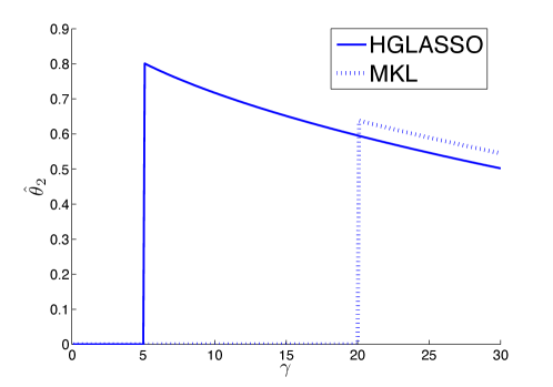
Figure 2: Estimators $\hat{\theta}^{(2)}$ as a function of $\gamma$. The curves are plotted only for the values of $\gamma$ which yield also $\hat{\theta}^{(1)}=0$ (different for HGLasso ($\gamma_{HGL}>5$) and MKL ($\gamma_{MKL}>20$)).

6 Mean Squared Error properties of Empirical Bayes Estimators

In this Section we evaluate the performance of an estimator $\hat{\theta}$ using its Mean Squared Error (MSE) i.e. its expected quadratic loss

$$\mbox{tr}\left[{\mathbb{E}}\left[\left.\left(\hat{\theta}-{\bar{\theta}}\right)\left(\hat{\theta}-{\bar{\theta}}\right)^{\top}\,\right|\,\lambda,\theta={\bar{\theta}}\right]\right],$$

where ${\bar{\theta}}$ is the “true” but unknown value of $\theta$. When we speak about “Bayes estimators” we think of estimators of the form $\hat{\theta}(\lambda):={\mathbb{E}}\left[\theta\,|\,y,\lambda\right]$ computed using the probabilistic model Fig. 1 with $\gamma$ fixed.

6.1 Properties using “orthogonal” regressors

We first derive the MSE formulas under the simplifying assumption of “orthogonal” regressors $(G^{\top}G=nI)$ and show that the Empirical Bayes estimator converges to an “optimal” estimator in terms of its MSE. This fact has close connections to the so called “Stein” estimators (James and Stein, 1961), (Stein, 1981), (Efron and Morris, 1973). The same optimality properties are attained, asymptotically, when the columns of $G$ are realizations of uncorrelated processes having the same variance. This is of interest in the system identification scenario considered in (Chiuso and Pillonetto, 2010a, b, 2011) since it arises when one performs identification with i.i.d. white noises as inputs. We then consider the more general case of correlated regressors (see Section 6.2) and show that essentially the same holds for a weighted version of the MSE.

In this section, it is convenient to introduce the following notation:

$${{\mathbb{E}}_{v}}[\,\cdot\,]:={\mathbb{E}}[\,\cdot\,|\,\lambda,\,\theta={\bar{\theta}}]\quad\mbox{and}\quad{\mbox{Var}_{v}}[\,\cdot\,]:={\mathbb{E}}[\,\cdot\,|\,\lambda,\,\theta={\bar{\theta}}].$$

We now report an expression for the MSE of the Bayes estimators $\hat{\theta}(\lambda):={\mathbb{E}}\left[\theta\,|\,y,\lambda\right]$ (proof follows from standard calculations and is therefore omitted).

Proposition 7

Consider the model (15) under the probabilistic model described in Fig. 1(b). The Mean Squared Error of the Bayes estimator $\hat{\theta}(\lambda):={\mathbb{E}}\left[\theta|y,\lambda\right]$ given $\lambda$ and $\theta={\bar{\theta}}$ is

$$MSE(\lambda) = \!\!\!\mbox{tr}\left[{{\mathbb{E}}_{v}}\left[(\hat{\theta}(\lambda)-\theta)(\hat{\theta}(\lambda)-\theta)^{\top}\right]\right]$$ (43)

$$= \!\!\!{\mbox{tr}}\left[\sigma^{2}\left(G^{\top}G+\sigma^{2}\Lambda^{-1}\right)^{-1}\left(G^{\top}G+\sigma^{2}\Lambda^{-1}{\bar{\theta}}{\bar{\theta}}^{\top}\Lambda^{-1}\right)\left(G^{\top}G+\sigma^{2}\Lambda^{-1}\right)^{-1}\right].$$

We can now minimize the expression for $MSE(\lambda)$ given in (43) with respect to $\lambda$ to obtain the optimal minimum mean squared error estimator. In the case where $G^{\top}G=nI$ this computation is straightforward and is recorded in the following proposition.

Corollary 8

Assume that $G^{\top}G=nI$ in Proposition 7. Then MSE($\lambda$) is globally minimized by choosing

$$\lambda_{i}=\lambda^{opt}_{i}:=\frac{\|{\bar{\theta}}^{(i)}\|^{2}}{k_{i}},\quad i=1,\dots,p.$$ (44)

Next consider the Maximum a Posteriori estimator of $\lambda$ again under the simplifying assumption $G^{\top}G=nI$. Note that, under the noninformative prior ($\gamma=0$), this Maximum a Posteriori estimator reduces to the standard Maximum (marginal) Likelihood approach to estimating the prior distribution of $\theta$. Consequently, we continue to call the resulting procedure Empirical Bayes (a.k.a. Type-II Maximum Likelihood, (Berger, 1985)).

Proposition 9

Consider model (15) under the probabilistic model described in Fig. 1(b), and assume that $G^{\top}G=nI$. Then the estimator of $\lambda_{i}$ obtained by maximizing the marginal posterior ${\bf p}(\lambda|y)$,

$$\{\hat{\lambda}_{1}(\gamma),...,\hat{\lambda}_{p}(\gamma)\}:=\arg\max_{{\lambda}\in{\mathbb{R}}_{+}^{p}}{\bf p}(\lambda|y)=\arg\max_{{\lambda}\in{\mathbb{R}}_{+}^{p}}\int{\bf p}(y,\theta|\lambda){\bf p}_{\gamma}(\lambda)\,d\theta,$$ (45)

is given by

$$\hat{\lambda}_{i}(\gamma)={\rm max}\left(0,\frac{1}{4\gamma}\left[\sqrt{k_{i}^{2}+8\gamma\|\hat{\theta}^{(i)}_{LS}\|^{2}}-\left(k_{i}+\frac{4\sigma^{2}\gamma}{n}\right)\right]\right)\ ,$$ (46)

where

$$\hat{\theta}_{LS}^{(i)}=\frac{1}{n}\left(G^{(i)}\right)^{\top}y$$

is the Least Squares estimator of the $i-$th block $\theta^{(i)}$. As $\gamma\rightarrow 0$ ($\gamma=0$ corresponds to an improper flat prior) the expression (46) yields:

$$\mathop{\rm lim}_{\gamma\rightarrow 0}\hat{\lambda}_{i}(\gamma)={\rm max}\left(0,\frac{\|\hat{\theta}_{LS}^{(i)}\|^{2}}{k_{i}}-\frac{\sigma^{2}}{n}\right)\ .$$ (47)

In addition, the probability ${\mathbb{P}}[\hat{\lambda}_{i}(\gamma)=0\,|\,\theta={\bar{\theta}}]$ of setting $\hat{\lambda}_{i}=0$ is given by

$${\mathbb{P}}[\hat{\lambda}_{i}(\gamma)=0\,|\,\theta={\bar{\theta}}]={\mathbb{P}}\left[\chi^{2}\left(k_{i},\|{\bar{\theta}}^{(i)}\|^{2}\frac{n}{\sigma^{2}}\right)\leq\left(k_{i}+2\gamma\frac{\sigma^{2}}{n}\right)\right]\ ,$$ (48)

where $\chi^{2}(d,\mu)$ denotes a noncentral $\chi^{2}$ random variable with $d$ degrees of freedom and noncentrality parameter $\mu$.

Note that the expression of $\hat{\lambda}_{i}(\gamma)$ in Proposition 9 has the form of a “saturation”. In particular, for $\gamma=0$, we have

$$\hat{\lambda}_{i}(0)={\rm max}(0,\hat{\lambda}_{i}^{*}),\quad\mbox{where}\quad\hat{\lambda}_{i}^{*}:=\frac{\|\hat{\theta}_{LS}^{(i)}\|^{2}}{k_{i}}-\frac{\sigma^{2}}{n}\ .$$ (49)

The following proposition shows that the “unsaturated” estimator $\hat{\lambda}_{i}^{*}$ is an unbiased and consistent estimator of $\lambda_{i}^{opt}$ which minimizes the Mean Squared Error while $\hat{\lambda}_{i}(0)$ is only asymptotically unbiased and consistent.

Corollary 10

Under the assumption $G^{\top}G=nI$, the estimator of $\hat{\lambda}^{*}:=\{\lambda_{1}^{*},..,\lambda_{p}^{*}\}$ in (49) is an unbiased and mean square consistent estimator of $\lambda^{opt}$ which minimizes the Mean Squared Error, while $\hat{\lambda}(0):=\{\lambda_{1}(0),..,\lambda_{p}(0)\}$ is asymptotically unbiased and consistent, i.e.:

$${\mathbb{E}}[\hat{\lambda}^{*}_{i}\,|\,\theta={\bar{\theta}}]=\lambda^{opt}_{i}\quad\mathop{\rm lim}_{n\rightarrow\infty}{\mathbb{E}}[\hat{\lambda}_{i}(0)\,|\,\theta={\bar{\theta}}]=\lambda^{opt}_{i}$$ (50)

and

$$\mathop{\rm lim}_{n\rightarrow\infty}\hat{\lambda}^{*}_{i}\mathop{=}^{m.s.}\lambda^{opt}_{i}\quad\mathop{\rm lim}_{n\rightarrow\infty}\hat{\lambda}_{i}(0)\mathop{=}^{m.s.}\lambda^{opt}_{i}$$ (51)

where $\displaystyle{\mathop{=}^{m.s.}}$ denotes convergence in mean square.

Remark 11

Note that if ${\bar{\theta}}^{(i)}=0$ the optimal value $\lambda_{i}^{opt}$ is zero. Hence (51) shows that asymptotically $\hat{\lambda}_{i}(0)$ converges to zero. However, in this case, it is easy to see from (48) that

$$\mathop{\rm lim}_{n\rightarrow\infty}{\mathbb{P}}[\hat{\lambda}_{i}(0)=0\,|\,\theta={\bar{\theta}}]<1.$$

There is in fact no contradiction between these two statements because one can easily show that for all $\epsilon>0$,

$${\mathbb{P}}[\hat{\lambda}_{i}(0)\in[0,\epsilon)\,|\,\theta={\bar{\theta}}]\mathop{\longrightarrow}^{n\rightarrow\infty}1.$$

In order to guarantee that $\mathop{\rm lim}_{n\rightarrow\infty}{\mathbb{P}}[\hat{\lambda}_{i}(\gamma)=0\,|\,\theta={\bar{\theta}}]=1$ one must chose $\gamma=\gamma_{n}$ so that $2\frac{\sigma^{2}}{n}\gamma_{n}\rightarrow\infty$, so that $\gamma_{n}$ grows faster than $n$. This is in line with the well known requirements for Lasso to be model selection consistent. In fact, Theorem 1 shows that the link between $\gamma$ and the regularization parameter $\gamma_{L}$ for Lasso is given by $\gamma_{L}=\sqrt{2\gamma}$. The condition $n^{-1}\gamma_{n}\rightarrow\infty$ translates into $n^{-1/2}\gamma_{Ln}\rightarrow\infty$, a well known condition for Lasso to be model selection consistent (Zhao and Yu, 2006; Bach, 2008).

The results obtained so far suggest that the Empirical Bayes resulting from HGLasso has desirable properties with respect to the MSE of the estimators. One wonders whether the same favorable properties are inherited by MKL or, equivalently, by GLasso. The next proposition shows that this is not the case. In fact, for ${\bar{\theta}}^{(i)}\neq 0$, MKL does not yield consistent estimators for $\lambda_{i}^{opt}$;in addition, for $\theta^{(i)}=0$, the probability of setting $\hat{\lambda}_{i}(\gamma)$ to zero (see equation (55)) is much smaller than that obtained using HGLasso (see equation (48)); this is also illustrated in Figure 3 (top). Also note that, as illustrated in Figure 3 (bottom), when the “true” $\theta$ is equal to zero, MKL tends to give much larger values of $\hat{\lambda}$ than those given by HGLasso. This results in larger values of $\|\hat{\theta}\|$ (see Figure 3).

Proposition 12

Consider model (15) under the probabilistic model described in Fig. 1(b), and assume $G^{\top}G=nI$. Then the estimator of $\lambda_{i}$ obtained by maximizing the joint posterior ${\bf p}(\lambda,\phi|y)$ (see equations (32) and (33)),

$$\{\hat{\lambda}(\gamma),...,\hat{\lambda}_{p}(\gamma)\}:=\arg\max_{{\lambda}\in{\mathbb{R}}_{+}^{p},{\phi}\in{\mathbb{R}}_{+}^{m}}{\bf p}(\lambda,\phi|y),$$ (52)

is given by

$$\hat{\lambda}_{i}(\gamma)={\rm max}\left(0,\frac{\|\hat{\theta}_{LS}^{(i)}\|}{\sqrt{2\gamma}}-\frac{\sigma^{2}}{n}\right),$$ (53)

where

$$\hat{\theta}_{LS}^{(i)}=\frac{1}{n}\left(G^{(i)}\right)^{\top}y$$

is the Least Squares estimator of the $i-$th block $\theta^{(i)}$ for $i=1,\dots,p$. For $n\rightarrow\infty$ the estimator $\hat{\lambda}_{i}(\gamma)$ satisfies

$$\mathop{\rm lim}_{n\rightarrow\infty}\hat{\lambda}_{i}(\gamma)\mathop{=}^{m.s.}\frac{\|{\bar{\theta}}^{(i)}\|}{\sqrt{2\gamma}}\ .$$ (54)

In addition, the probability ${\mathbb{P}}[\hat{\lambda}_{i}(\gamma)=0\,|\,\theta={\bar{\theta}}]$ of setting $\hat{\lambda}_{i}(\gamma)=0$ is given by

$${\mathbb{P}}_{\theta}[\hat{\lambda}_{i}(\gamma)=0\,|\,\theta={\bar{\theta}}]={\mathbb{P}}\left[\chi^{2}\left(k_{i},\|{\bar{\theta}}^{(i)}\|^{2}\frac{n}{\sigma^{2}}\right)\leq 2\gamma\frac{\sigma^{2}}{n}\right]\ .$$ (55)

Note that the limit of the MKL estimators $\hat{\lambda}_{i}(\gamma)$ as $n\rightarrow\infty$ depends on $\gamma$. Therefore, using MKL (GLASSO), one cannot hope to get consistent estimators of $\lambda_{i}^{opt}$. Indeed, for $\|{\bar{\theta}}^{(i)}\|^{2}\neq 0$, consistency of $\hat{\lambda}_{i}(\gamma)$ requires $\gamma\rightarrow\frac{k^{2}_{i}}{2\|{\bar{\theta}}^{(i)}\|^{2}}$, which is a circular requirement.

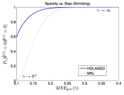
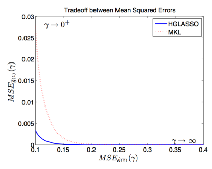
Figure 3: This plot has been generated assuming that there are two blocks ($p=2$) of dimension $k_{1}=k_{2}=10$ with $\bar{\theta}^{(1)}=0$ and all the components of the true $\bar{\theta}^{(2)}\in{\mathbb{R}}^{10}$ set to one. The matrix $G$ equal to the identity, so that the output dimension ($y\in{\mathbb{R}}^{n}$) is $n=20$; the noise variance equal to $0.1$. Left: probability of setting $\hat{\theta}^{(1)}$ to zero vs Mean Squared Error in $\hat{\theta}^{(2)}$. Curves are parametrized in $\gamma\in[0,+\infty)$. Right: Mean Squared Error in $\hat{\theta}^{(1)}$ vs Mean Squared Error in $\hat{\theta}^{(2)}$. Curves are parametrized in $\gamma\in[0,+\infty)$.

6.2 Asymptotic properties using general regressors

In this subsection, we replace the deterministic matrix $G$ with $G_{n}(\omega)$, where $G_{n}(\omega)$ represents an $n\times m$ matrix defined on the complete probability space $(\Omega,\mathcal{B},{\mathbb{P}})$ with $\omega$ a generic element of $\Omega$ and $\mathcal{B}$ the sigma field of Borel regular measures. In particular, the rows of $G_{n}$ are independent realizations from a zero-mean random vector with positive definite covariance $\Psi$. We will also assume that the (mild) assumptions for the convergence in probability of $G_{n}^{\top}G_{n}/n$ to $\Psi$, as $n$ goes to $\infty$, are satisfied, see e.g. (Loève, 1963).
As in the previous part of this section, $\lambda$ and $\theta$ are seen as parameters, and the “true” value of $\theta$ is ${\bar{\theta}}$. Hence, all the randomness present in the next formulas comes only from $G_{n}$ and the measurement noise. Below, the dependence of $\Sigma_{y}(\lambda)$ on $G_{n}$, and hence of $n$, is omitted to simplify the notation. Furthermore, $\longrightarrow_{p}$ denotes convergence in probability.

Theorem 13

For known $\gamma$ and conditional on $\theta={\bar{\theta}}$, define

$$\hat{\lambda}^{n}=\arg\min_{{\lambda}\in\mathcal{C}\bigcap{\mathbb{R}}_{+}^{p}}\frac{1}{2}\log\det(\Sigma_{y}(\lambda))+\frac{1}{2}y^{\top}\Sigma_{y}^{-1}(\lambda)y+\gamma\sum_{i=1}^{p}{\lambda}_{i},$$ (56)

where $\mathcal{C}$ is any $p$-dimensional ball with radius larger than $\max_{i}\frac{\|{\bar{\theta}}^{(i)}\|^{2}}{k_{i}}$.
Then, we have

$$\hat{\lambda}_{i}^{n}\longrightarrow_{p}\frac{-k_{i}+\sqrt{k_{i}^{2}+8\gamma\|{\bar{\theta}}^{(i)}\|^{2}}}{4\gamma}\quad \gamma>0 \|\theta^{(i)}\|>0$$ if    and  , (57)

$$\hat{\lambda}_{i}^{n}\longrightarrow_{p}\frac{\|{\bar{\theta}}^{(i)}\|^{2}}{k_{i}}\quad \gamma=0 \|\theta^{(i)}\|>0$$ if    and  , and (58)

$$\hat{\lambda}_{i}^{n}\longrightarrow_{p}0\quad \gamma\geq 0 \|\theta^{(i)}\|=0$$ if    and  . (59)

We now show that, when $\gamma=0$, the above result relates to the problem of minimizing the MSE of the $i$-th block with respect to $\lambda_{i}$, with all the other components of $\lambda$ coming from $\hat{\lambda}^{n}$. If $\hat{\theta}^{(i)}_{n}(\lambda)$ denotes the $i$-th component of the HGLasso estimate of $\theta$ defined in (21), our aim is to optimize the objective

$$MSE_{n}(\lambda_{i}):=\mbox{tr}\left[{{\mathbb{E}}_{v}}\left[(\hat{\theta}_{n}^{(i)}(\lambda)-\theta^{(i)})(\hat{\theta}_{n}^{(i)}(\lambda)-\theta^{(i)})^{\top}\right]\right]\quad\mbox{with}\quad\lambda_{j}=\bar{\lambda}_{j}^{n}\quad\mbox{for}\quad j\neq i$$

where is $\bar{\lambda}_{j}^{n}$ is any sequence satisfying condition

$$\begin{array}[]{c}\displaystyle{\mathop{\rm lim}_{n\rightarrow\infty}}\;f_{n}=+\infty\quad{\rm where}\quad f_{n}:=\displaystyle{\mathop{\rm min}_{j\in I_{1}}}\;n\lambda_{j}^{n},\end{array}$$ (60)

where $I_{1}:=\{j\,:\,j\neq i\mbox{ and }\bar{\theta}^{(j)}\neq 0\}$ (condition (60) appears again in the Appendix as (94)). Note that, in particular, $\bar{\lambda}_{j}^{n}=\hat{\lambda}_{j}^{n}$ in (56) satisfy (60) in probability.

In the following lemma, whose proof is in the Appendix, we introduce a change of variables that is key for our understanding of the asymptotic properties of these more general regressors.

Lemma 14

Fix $i\in\{1,\dots,p\}$ and consider the decomposition

$$\begin{array}[]{rcl}y&=&G^{(i)}\theta^{(i)}+\sum_{j=1,j\neq i}^{p}G^{(j)}\theta^{(j)}+v\\ &=&G^{(i)}\theta^{(i)}+\bar{v}\end{array}$$ (61)

of the linear measurement model (15) and assume (88) holds. Define

$$\Sigma_{\bar{v}}:=\sum_{j=1,j\neq i}^{p}G^{(j)}\left(G^{(j)}\right)^{\top}\lambda_{j}+\sigma^{2}I$$

and assume that $\lambda_{j}$ finite $\forall j\neq i$. Consider now the singular value decomposition

$$\frac{\Sigma_{\bar{v}}^{-1/2}G^{(i)}}{\sqrt{n}}=U_{n}^{(i)}D_{n}^{(i)}\left(V_{n}^{(i)}\right)^{\top}$$ (62)

where each $D_{n}^{(i)}=\mbox{diag}(d_{k,n}^{(i)})$ is $k_{i}\times k_{i}$ diagonal matrix. Then (61) can be transformed into the equivalent linear model

$$\begin{array}[]{rcl}z_{n}^{(i)}&=&D_{n}^{(i)}\beta_{n}^{(i)}+\epsilon_{n}^{(i)},\end{array}$$ (63)

where

$$\begin{array}[]{ccc}z_{n}^{(i)}:=\left(U_{n}^{(i)}\right)^{\top}\frac{\Sigma_{\bar{v}}^{-1/2}y}{\sqrt{n}}=(z_{k,n}^{(i)}),&\beta_{n}^{(i)}:=\left(V_{n}^{(i)}\right)^{\top}\theta^{(i)}=(\beta_{k,n}^{(i)}),&\epsilon_{n}^{(i)}:=\left(U_{n}^{(i)}\right)^{\top}\frac{\Sigma_{\bar{v}}^{-1/2}\bar{v}}{\sqrt{n}}=(\epsilon_{k,n}^{(i)}),\end{array}$$ (64)

and $D_{n}^{(i)}$ is uniformly (in $n$) bounded and bounded away from zero.

Lemma 14 shows that we can consider the transformed linear model associated with the $i$-th block, i.e.

$$\begin{array}[]{rcl}z_{k,n}^{(i)}&=&d_{k,n}^{(i)}\beta_{k,n}^{(i)}+\epsilon_{k,n}^{(i)},\quad k=1,\ldots,k_{i},\end{array}$$ (65)

where all the three variables on the RHS depend on $\bar{\lambda}_{j}^{n}$ for $j\neq i$. In particular, the vector $\beta_{n}^{(i)}$ consists of an orthonormal transformation of $\theta^{(i)}$ while the $d_{k,n}^{(i)}$ are all bounded below in probability. In addition, by letting

$${{\mathbb{E}}_{v}}\left[\epsilon_{k,n}^{(i)}\right]=m_{k,n},\quad{{\mathbb{E}}_{v}}\left[(\epsilon_{k,n}^{(i)}-m_{k,n})^{2}\right]=\sigma^{2}_{k,n},$$ (66)

we also know from Lemma 17 (see equations (96) and (97)) that, provided $\bar{\lambda}_{j}^{n}$ $(j\neq i)$ satisfy condition (60), both $m_{k,n}$ and $\sigma^{2}_{k,n}$ tend to zero (in probability) as $n$ goes to $\infty$. Then, after simple computations, one finds that the $MSE$ relative to $\beta_{n}^{(i)}$ is the following random variable whose statistics depend on $n$:

$$MSE_{n}(\lambda_{i})=\sum_{k=1}^{k_{i}}\frac{\beta_{k,n}^{2}+n\lambda_{i}^{2}d_{k,n}^{2}(m_{k,n}^{2}+\sigma^{2}_{k,n})-2\lambda_{i}d_{k,n}m_{k,n}\beta_{k,n}}{(1+n\lambda_{i}d_{k,n}^{2})^{2}}\quad\mbox{with}\quad\lambda_{j}=\bar{\lambda}_{j}^{n}\quad\mbox{for}\quad j\neq i.$$

Above, except for $\lambda_{i}$, the dependence on the block number $i$ was omitted to improve readability.
Now, let $\breve{\lambda}_{i}^{n}$ denote the minimizer of the following weighted version of the $MSE_{n}(\lambda_{i})$:

$$\breve{\lambda}_{i}^{n}=\arg\min_{\lambda\in{\mathbb{R}}_{+}}\sum_{k=1}^{k_{i}}d_{k,n}^{4}\frac{\beta_{k,n}^{2}+n\lambda_{i}^{2}d_{k,n}^{2}(m_{k,n}^{2}+\sigma^{2}_{k,n})-2\lambda_{i}d_{k,n}m_{k,n}\beta_{k,n}}{(1+n\lambda_{i}d_{k,n}^{2})^{2}}.$$

Then, the following result holds.

Proposition 15

For $\gamma=0$ and conditional on $\theta={\bar{\theta}}$, the following convergences in probability hold

$$\lim_{n\mapsto\infty}\breve{\lambda}_{i}^{n}=\frac{\|{\bar{\theta}}^{(i)}\|^{2}}{k_{i}}=\lim_{n\mapsto\infty}\hat{\lambda}_{i}^{n}\ ,\quad i=1,2,\ldots,p.$$ (67)

The proof follows arguments similar to those used in last part of the proof of Theorem 13, see also proof of Theorem 6 in Aravkin et al. (2012), and is therefore omitted.

We can summarize the two main findings reported in this subsection as follows. As the number of measurements go to infinity:

1. regardless of the value of $\gamma$, the proposed estimator will correctly set to zero only those $\lambda_{i}$ associated with null blocks;

2. when $\gamma=0$, (58) and (59) provide the asymptotic properties of ARD, showing that the estimate of $\lambda_{i}$ will converge to the energy of the $i$-th block (divided by its dimension). This same value also represents the asymptotic minimizer of a weighted version of the $MSE$ relative to the $i$-th block. In particular, the weights change over time, being defined by singular values $d_{k,n}^{(i)}$, (raised at fourth power) that depend on the trajectories of the other components of $\lambda$.

6.2.1 Marginal likelihood and weighted MSE: perturbation analysis

We now provide some additional insights on point 2 above, investigating why the weights $d_{k,n}^{4}$ may lead to an effective strategy for hyperparameter estimation.
For our purposes, just to simplify the notation, let us consider the case of a single $m$-dimensional block. In this way, $\lambda$ becomes a scalar and the noise $\epsilon_{k,n}$ in (65) is zero-mean of variance $1/n$.
Under the stated assumptions, the $MSE$ weighted by $d_{k,n}^{\alpha}$, with $\alpha$ an integer, becomes

$$\sum_{k=1}^{m}d_{k,n}^{\alpha}\frac{n^{-1}\beta_{k,n}^{2}+\lambda^{2}d_{k,n}^{2}}{(n^{-1}+\lambda d_{k,n}^{2})^{2}},$$ (68)

whose partial derivative with respect to $\lambda$, apart from the scale factor $2/n$, is

$$F_{\alpha}(\lambda)=\sum_{k=1}^{m}d_{k,n}^{\alpha+2}\frac{\lambda-\beta_{k,n}^{2}}{(n^{-1}+\lambda d_{k,n}^{2})^{3}}.$$ (69)

Let $\beta_{k}=\lim_{n\mapsto\infty}\beta_{k,n}$ and $d_{k}=\lim_{n\mapsto\infty}d_{k,n}$ . When $n$ tends to infinity, arguments similar to those introduced in the last part of the proof of Theorem 13 show that, in probability, the zero of $F_{\alpha}$ becomes

$$\breve{\lambda}(\alpha)=\frac{\sum_{k=1}^{m}d_{k}^{\alpha-4}\beta_{k}^{2}}{\sum_{k=1}^{m}d_{k}^{\alpha-4}}.$$ (70)

Notice that the formula above is a generalization of the first equality in (67) that was obtained by setting $\alpha=4$. However, for practical purposes, the above expressions are not useful since the true values of $\beta_{k,n}$ and $\beta_{k}$ depend on the unknown ${\bar{\theta}}$. One can then consider a noisy version of $F_{\alpha}$ obtained by replacing $\beta_{k,n}$ with its least squares estimate, i.e.

$$\tilde{F}_{\alpha}(\lambda)=\sum_{k=1}^{m}d_{k,n}^{\alpha+2}\frac{\lambda-\left(\beta_{k,n}+\frac{v_{k,n}}{\sqrt{n}d_{k,n}}\right)^{2}}{(n^{-1}+\lambda d_{k,n}^{2})^{3}},$$ (71)

where the random variable $v_{k,n}$ is of unit variance. For large $n$, considering small additive perturbations around the model $z_{k}=d_{k}\beta_{k}$, it is easy to show that the minimizer tends to the following perturbed version of $\breve{\lambda}$:

$$\breve{\lambda}(\alpha)+2\frac{\sum_{k=1}^{m}d_{k}^{\alpha-5}\beta_{k}v_{k,n}}{\sqrt{n}\sum_{k=1}^{m}d_{k}^{\alpha-4}}.$$ (72)

It remains to choose the value of $\alpha$ that should enter the above formula. This is far from trivial since the optimal value (minimizing MSE) depends on the unknown $\beta_{k}$. On one hand, it would seem advantageous to have $\alpha$ close to zero. In fact, $\alpha=0$ relates $\breve{\lambda}$ to the minimization of the $MSE$ on $\theta$ while $\alpha=2$ minimizes the $MSE$ on the output prediction, see the discussion in Section 4 of Aravkin et al. (2012). On the other hand, a larger value for $\alpha$ could help in controlling the additive perturbation term in (72) possibly reducing its sensitivity to small values of $d_{k}$. For instance, the choice $\alpha=0$ introduces in the numerator of (72) the term $\beta_{k}/d_{k}^{5}$. This can make numerically unstable the convergence towards $\breve{\lambda}$, leading to poor estimates of the regularization parameters, as e.g. described via simulation studies in Section 5 of Aravkin et al. (2012). In this regard, the choice $\alpha=4$ appears interesting: it sets $\breve{\lambda}$ to the energy of the block divided by $m$, removing the dependence of the denominator in (72) on $d_{k}$. In particular, it reduces (72) to

$$\frac{\|\beta\|^{2}}{m}+\frac{2}{m}\sum_{k=1}^{m}\frac{\beta_{k}v_{k,n}}{\sqrt{n}d_{k}}=\sum_{k=1}^{m}\frac{\beta_{k}^{2}}{m}\left(1+2\frac{v_{k,n}}{\beta_{k}\sqrt{n}d_{k}}\right).$$ (73)

It is thus apparent that $\alpha=4$ makes the perturbation on $\frac{\beta_{k}^{2}}{m}$ dependent on $\frac{v_{k,n}}{\beta_{k}\sqrt{n}d_{k}}$ that is the relative reconstruction error on $\beta_{k}$. This appears a reasonable choice to account for the ill-conditioning possibly affecting least-squares.

Interestingly, for large $n$, this same philosophy is followed by the marginal likelihood procedure for hyperparameter estimation up to first-order approximations. In fact, under the stated assumptions, apart from constants, the minus two log of the marginal likelihood is

$$\sum_{k=1}^{m}\log(n^{-1}+\lambda d_{k,n}^{2})+\frac{z_{k,n}^{2}}{n^{-1}+\lambda d_{k,n}^{2}},$$ (74)

whose partial derivative w.r.t. $\lambda$ is

$$\sum_{k=1}^{m}\frac{d_{k,n}^{4}+n^{-1}d_{k,n}^{2}-z_{k,n}^{2}d_{k,n}^{2}}{(n^{-1}+\lambda d_{k,n}^{2})^{2}}.$$ (75)

As before, we consider small perturbations around $z_{k}=d_{k}\beta_{k}$ to find that a critical point occurs at

$$\sum_{k=1}^{m}\frac{\beta_{k}^{2}}{m}\left(1+2\frac{v_{k,n}}{\beta_{k}\sqrt{n}d_{k}}\right),$$ (76)

which is exactly the same minimizer reported in (73).

7 Three variants of HGLasso and their implementation

In this section we discuss the implementation of our HGLasso approach. In particular, the results introduced in the previous section point out some distinctive features of HGLasso with respect to GLasso (MKL). In fact, we have shown that HGLasso relies upon an estimator for the hyperparameter $\lambda$ having some favorable properties in terms of MSE minimization. In addition, sparsity can be induced using a smaller value for $\gamma$ than that needed by GLasso. This is an important point since we have seen that nice MSE properties are obtained optimizing the marginal posterior of $\lambda$ with $\gamma$ close to zero.

On the other hand, a drawback of the HGLasso is that it requires the solution to a non-convex optimization problem in a possibly high-dimensional space. We show that this problem can be faced by introducing a variant of HGLasso where only one scalar variable is involved in the optimization process. In addition, this procedure is able to promote greater sparsity than the full version of HGLasso while continuing to accurately reconstruct the nonzero blocks. This new computational scheme, which we call HGLa, relies on the combination of marginal likelihood optimization and Bayesian forward selection equipped with cross validation to select $\gamma$. It is introduced in the following subsections together with two other versions that will be called HGLb and HGLc. The following two subsections are instrumental to the introduction of the three algorithms.

7.1 Bayesian Forward Selection

In this section we introduce a forward-selection procedure which will be useful to define the computationally efficient version of the HGLasso estimator. Hereafter, we use $y_{tr}$ and $y_{val}$ to indicate the output data contained in the training and validation data set, respectively. This also induces a natural partition of $G$ into $G_{tr}$ and $G_{val}$. In order to obtain an estimator of $\lambda$ we consider the constraint $\kappa=\lambda_{1}=\lambda_{2}=\ldots=\lambda_{p}$ and treat $\kappa$ as a deterministic hyperparameter whose knowledge makes the covariance $\Sigma_{y_{tr}}$ of the data $y_{tr}$ completely known. Therefore we set:

$$\begin{array}[]{rcl}\hat{\kappa}&:=&\displaystyle{\arg\min_{\kappa\in{\mathbb{R}}_{+}}\frac{1}{2}\log\det(\Sigma_{y_{tr}})+\frac{1}{2}y_{tr}^{\top}\Sigma_{y_{tr}}^{-1}y_{tr}}\end{array}$$ (77)

Now, we consider again the Bayesian model in Fig. 1(b), where all the components of $\lambda$ are fixed to $\hat{\kappa}$ while $\gamma$ may vary on a grid $C$ built around $\hat{\kappa}^{-1}$. The forward-selection procedure is then designed as follows; for each value of $\gamma$ in the grid $C$ let $I\subseteq\{1,2,..,p\}$ be the subset of currently selected groups and, using the Bayesian model in Fig. 1(b) (see also (2.2)-(8)), define the marginal log posterior

$$L(I,\kappa,\gamma):={\rm log}\left[p_{\gamma}(\tilde{\lambda}_{I}|y_{tr})\right]$$ (78)

$\tilde{\lambda}_{I}:=[\tilde{\lambda}_{I,1},...,\tilde{\lambda}_{I,p}]$ and $\tilde{\lambda}_{I,i}=\hat{\kappa}$ if $i\in I$ and $\tilde{\lambda}_{I,i}=0$ otherwise. Then, for each value of $\gamma$ in the grid $C$, perform the following procedure:

• initialize $I(\gamma):=\emptyset$

• repeat the following procedure:

  • for $j\in\{1,..,p\}\setminus I(\gamma)$, define $I_{j}^{{}^{\prime}}(\gamma):=I(\gamma)\cup{j}$ and compute $L(I_{j}^{{}^{\prime}}(\gamma);\hat{\kappa},\gamma)$.

  • select

    $$\bar{j}:=\mathop{arg\;max}_{j\in\{1,..,p\}\setminus I(\gamma)}L(I_{j}^{{}^{\prime}}(\gamma);\hat{\kappa},\gamma)-L(I(\gamma);\hat{\kappa},\gamma)$$

  • if $L(I_{\bar{j}}^{{}^{\prime}}(\gamma);\hat{\kappa},\gamma)-L(I(\gamma);\hat{\kappa},\gamma)>0$
    set $I(\gamma):=I^{{}^{\prime}}_{\bar{j}}(\gamma)$ and go back to (a)
    else
    finish.

Note that, for each $\gamma$ in the grid, the set $I(\gamma)$ contains the indexes of selected variables different from zero. Let $\hat{\gamma}$ denote the value of $\gamma$ from the grid that yields the best prediction on the validation data set $y_{val}$, i.e.

$$\hat{\gamma}=\arg\min_{\gamma\in C}\|y_{val}-G_{val}{\theta}_{HGL}(\tilde{\lambda}_{I(\gamma)})\|$$

and set $I_{FS}=I(\hat{\gamma})$.

7.2 Projected Quasi-Newton Method

The objective in (19) is a differentiable function of $\lambda$. The computation of its derivative requires a one time evaluation of the matrices $G^{(i)}G^{(i)^{\top}},\ i=1,\dots,p$. However, for each new value of $\lambda$, the inverse of the matrix $\Sigma_{y}(\lambda)$ also needs to be computed. Hence, the evaluation of the objective and its derivative may be costly since it requires computing the inverse of a possibly large matrix as well as large matrix products. On the other hand, the dimension of the parameter vector $\lambda$ can be small, and projection onto the feasible set is trivial.

We experimented with several methods available in the Matlab package minConf to optimize (19). In these experiments, the fastest method was the limited memory projected quasi-Newton algorithm detailed in (Schmidt et al., 2009). It uses L-BFGS updates to build a diagonal plus low-rank quadratic approximation to the function, and then uses the Projected Quasi-Newton Method to minimize a quadratic approximation subject to the original constraints to obtain a search direction. A backtracking line search is applied to this direction terminating at a step-size satisfying a Armijo-like sufficient decrease condition. The efficiency of the method derives in part from the simplicity of the projections onto the feasible region. We have also implemented the re-weighted method described in (Wipf and Nagarajan, 2007). In all the numerical experiments described below, we have assessed that it returns results virtually identical to those achieved by our method, with a similar computational effort. It is worth recalling that both the projected quasi-Newton method and the re-weighted approach guarantee only converge to a stationary point of the objective.

7.3 The three variants of HGLasso

We consider the three version of HGLasso.

• HGLa: Output data $y$ are split in a training and validation data set. The optimization problem (77) is solved using only the training data obtaining $\hat{\kappa}$. The regularization parameter $\gamma$ is estimated using the forward-selection procedure described in the previous subsection equipped with cross-validation. This procedure also returns the set $I_{FS}$ containing the indexes of the selected variables different from zeros. This index set gives an estimate $\hat{\lambda}_{FS}$ of the hyperparameter vector, whose components are equal to $\hat{\kappa}$ for $i\in I_{FS}$, and zero otherwise . Finally, $\hat{\theta}_{HGL}$ is estimated by the formula given in (21), ${\mathbb{E}}(\theta\,|\,y,\,\hat{\lambda}_{FS})=\mbox{blockdiag}((\hat{\lambda}_{FS})_{i}I_{k_{i}})G^{\top}\Sigma_{y}(\hat{\lambda}_{FS})^{-1}y$, using all the available data, i.e. the union of the training and validation data sets.

• HGLb: The optimization problem (19) is solved using the Projected Quasi-Newton method with starting point defined by the $\hat{\lambda}_{FS}$ returned by HGLa. The regularization parameter $\gamma$ is set to the estimate obtained by HGLa, $\hat{\gamma}$. Once the new estimate of $\lambda$ is obtained, $\hat{\theta}_{HGL}$ is computed using (21).

• HGLc: This estimator performs the same operations as HGLb except that the components of $\lambda$ set to zero by HGLa are kept at zero, i.e. $\lambda_{i}=0,\ i\notin I_{FS}$. In addition, the regularization parameter $\gamma$ is set to zero in order to obtain the MSE properties in the reconstruction of the blocks different from zero established in Proposition 15. Hence, the problem (19) is optimized with $\gamma=0$ and only over those $\lambda_{i}$ for $i\in I_{FS}$.

8 Numerical experiments

8.1 Simulated data

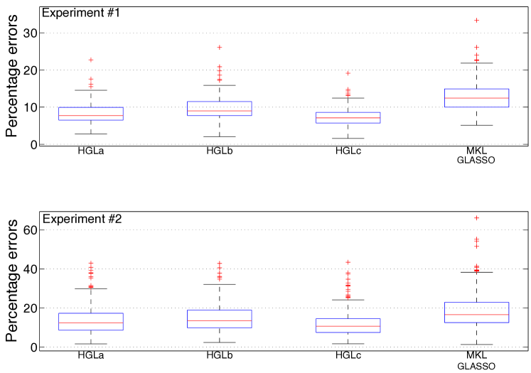
Figure 4: Comparison with MKL/GLasso (section 8.1). Boxplot of the percentage errors in the reconstruction of $\theta$ (top) obtained by the 4 estimators after the 300 Monte Carlo runs in Experiment $\#1$ (top panel) and $\#2$ (bottom panel).

We consider two Monte Carlo studies of $300$ runs each on the linear model (15) with $p=10$ groups, each composed of $k_{i}=4$ parameters, and $n=100$. For each run, $5$ of the $\theta^{(i)}$ groups are set to zero, one is always taken different from zero while each of the remaining $4$ $\theta^{(i)}$ groups are set to zero with probability $0.5$. The components of every $\theta^{(i)}$ block not set to zero are independent realizations from a uniform distribution on $[-a_{i},a_{i}]$ where $a_{i}$ is an independent realization (one for each block) from a uniform distribution on $[0,100]$. The value of $\sigma^{2}$ is equal to the variance of the noiseless output divided by 25. The noise variance is assumed unknown and its estimate is determined at each run as the sum of the residuals coming from the least squares estimate divided by $n-m$. The two experiments differ in the way the columns of $G$ are generated at each run. In the first experiment, the entries of $G$ are independent realizations of zero mean unit variance Gaussian noise. In the second experiment the columns of $G$ are correlated, being defined at every run by

$$G_{i,j}=G_{i,j-1}+0.2v_{i,j-1},\quad i=1,..,n,\quad j=2,..,m$$

$$v_{i,j}\sim{\cal N}(0,1)$$

where $v_{i,j}$ are i.i.d. (as $i$ and $j$ vary) zero mean unit variance Gaussian and $G_{i,1}$ are i.i.d. zero mean unit variance Gaussian random variables. Note that correlated inputs renders the estimation problem more challenging.

We compare the performance of the following $4$ estimators.

• HGLa,HGLb,HGLc: These are the three variants of our HGLasso procedure defined at the end of Section 7. The data is split into training and validation data sets of equal size and the grid $C$ used by the cross validation procedure to select $\gamma$ contains 30 elements logarithmically distributed between $10^{-2}\times\hat{\kappa}^{-1}$ and $10^{4}\times\hat{\kappa}^{-1}$

• MKL (GLasso): The regularization parameter is determined via cross validation, splitting the data set in two segments of the same size and testing a finite number of parameters from a grid with $30$ elements logarithmically distributed between $10^{-2}\times\hat{\gamma}$ and $10^{4}\times\hat{\gamma}$ where $\hat{\gamma}$ is the regularization parameter adopted by the three HLasso procedures. Finally, MKL (GLasso) is reapplied to the full data set fixing the regularization parameter to its estimate.

The $4$ estimators are compared using the two performance indexes listed below:

1. Percentage estimation error: this is computed at each run as

   $$100\times\frac{\|\theta-\hat{\theta}\|}{\|\theta\|}\,\%$$ (79)

   where $\hat{\theta}$ is the estimate of $\theta$.

2. Percentage of the blocks equal to zero correctly set to zero by the estimator after the $300$ runs.

The top and bottom panel of Fig. 4 displays the boxplots of the 300 percentage errors obtained by the 4 estimators in the first and second experiment, respectively. It is apparent that all of the three versions of HGLasso outperform GLasso.

In Table 1 we report the sparsity index. One can see that in the first and second experiment the first and third version of HGLasso obtain the remarkable performance of around $99\%$ of blocks correctly set to zero, while the second version obtains a value close to $76\%$. Instead, in the two experiments GLasso (MKL) correctly set to zero no more than $40\%$ of the blocks. This result, which can appear surprising, is explained by the arguments in Sections 5 and 6; in a nutshell, GLasso trades sparsity for shrinkage. The value of the regularization parameter $\gamma$ needed to avoid oversmoothing is not sufficiently large to induce “enough” sparsity. This drawback does not affect our new nonconvex estimators. These estimators have the additional advantage of selecting the regularization parameters leading to more favorable MSE properties for the reconstruction of the non zero blocks, as discussed in Section 6 and illustrated in Section 5 in a simplified scenario.

	HGLa	HGLb	HGLc	MKL (GLasso)
Experiment $\#1$	$99.2\%$	$76.1\%$	$99.2\%$	$36.1\%$
Experiment $\#2$	$99.0\%$	$76.5\%$	$99.0\%$	$39.5\%$

Table 1: Comparison with MKL/GLasso (section 8.1). Percentage of the $\theta^{(i)}$ equal to zero correctly set to zero by the four estimators.

8.1.1 Testing a variant of HGLa

To better point out the role played by $\gamma$ in our numerical schemes, we have also considered a variant of HGLa where $\gamma$ is always set to 0 and the parameter $\sigma^{2}$ is used to induce sparsity. More precisely, the only difference with respect to HGLa is that, after obtaining $\sigma^{2}$ from least squares and determining $\hat{\kappa}$, $\sigma^{2}$ is re-estimated using the forward-selection procedure equipped with cross-validation.
For the sake of comparison, we have considered 3 Monte Carlo studies of 300 runs. Data are generated as in the second experiment described above except that the 3 cases exploit different values of $\sigma^{2}$ equal to the noiseless output variance divided by $5$ (case a), $2$ (case b) or $1$ (case c). Table 2 reports the mean of the 300 percentage errors while Table 3 reports the sparsity index.
It is apparent that the variant of HGLa performs quite well, but HGLa outperforms it in all the experiments. These results can be given the following interpretation. When one adopts HGLa, the ”high level” of the Bayesian network depicted in Fig. 1 (b) (represented by $\gamma$) is used to to induce sparsity with the parameters entering the lower level of the Bayesian network that need not to be changed. Thus, $\theta$ is eventually reconstructed adopting the $\sigma^{2}$ estimated from data and the $\lambda$ determined by marginal likelihood optimization, thus possibly exploiting the MSE properties reported in Proposition 15. When $\gamma$ is instead set to $0$, the estimator has to trade sparsity and shrinkage using a less flexible structure. In particular, the lower level of the Bayesian network is now also in charge of enforcing sparsity and this can be done only increasing $\sigma^{2}$, possibly loosing performance in terms of MSE.

	HGLa	Variant of HGLa
Experiment $\#2$ (case a)	$12.2\%$	$15.6\%$
Experiment $\#2$ (case b)	$30.1\%$	$39.2\%$
Experiment $\#2$ (case c)	$61.5\%$	$73.8\%$

Table 2: Comparison with the variant of HGLa (section 8.1.1). Mean of the percentage errors in the reconstruction of $\theta$ obtained by HGLa and by the variant of HGLa where sparsity is induced by $\sigma^{2}$.

	HGLa	Variant of HGLa
Experiment $\#2$ (case a)	$99.2\%$	$93.1\%$
Experiment $\#2$ (case b)	$96.2\%$	$86.5\%$
Experiment $\#2$ (case c)	$88.1\%$	$71.4\%$

Table 3: Comparison with the variant of HGLa (section 8.1.1). Percentage of the $\theta^{(i)}$ equal to zero correctly set to zero by HGLa and by the variant of HGLa where sparsity is induced by $\sigma^{2}$.

8.2 Comparison with Adaptive Lasso

In this section we compare the performance of HGLa with that obtainable by the Adaptive Lasso (AdaLasso) procedure introduced in (Zou, 2006). In particular, we consider an example taken from (Zou, 2006) where the components of $\theta$ are $\{3,1.5,0,0,2,0,0,0\}$ and each component represents a group (block size is equal to 1). The rows of the design matrix $G$ are independent realizations from a zero mean Gaussian vector, with $(i,j)$-entry of its covariance equal to $\beta^{|i-j|}$. To be more specific, we consider 6 Monte Carlo studies, each of 200 runs, where at each run $\beta$ is drawn uniformly from the open interval $(0.5,1)$. The 6 experiments then differ in the number of data used to reconstruct $\theta$ (20 or 60) and in the variance of the Gaussian measurement noise ($\sigma^{2}$=1, 9 or 16). We implemented HGLa and Lasso as described in the previous subsection. For what regards AdaLasso, as in (Zou, 2006) we exploited two-dimensional cross validation to estimate the regularization parameter and the variable $\eta$ defining the weights. In particular, the latter were set to the inverse of the absolute value of the least squares estimates raised at $\eta$, where $\eta$ may vary on the grid $[0.5,1,\ldots,4]$.
Results are summarized in Table 4, that reports the mean of the 200 percentage errors, and in Table 5, where the sparsity index is displayed. One can notice that HGLa outperforms Lasso and AdaLasso, achieving both a smaller reconstruction error and a better sparsity index. To further illustrate this fact, at each Monte Carlo run we have also computed the Euclidean norm of the estimates of the null components of $\theta$ returned by the three estimators, divided by the norm of the true $\theta$. Since the number of null components of $\theta$ is 5 and the overall number of Monte Carlo runs is 1200, 6000 values were stored. Fig. 5 plots them (as a function of the Monte Carlo run) as points when the estimated value is different from zero (no point is displayed if the corresponding value is zero). It is apparent that in this example HGLa correctly detects the null components of $\theta$ more frequently than Lasso and AdaLasso, also providing a smaller reconstruction error when a component is not set to zero.

	HGLa	Lasso	AdaLasso
Exp. $\#1$ (n=20, $\sigma^{2}=1$)	$30.2\%$	$34.5\%$	$38.2\%$
Exp. $\#2$ (n=60, $\sigma^{2}=1$)	$12.1\%$	$15.3\%$	$17.1\%$
Exp. $\#3$ (n=20, $\sigma^{2}=9$)	$68.5\%$	$81.2\%$	$100.1\%$
Exp. $\#4$ (n=60, $\sigma^{2}=9$)	$43.1\%$	$46.3\%$	$56.6\%$
Exp. $\#5$ (n=20, $\sigma^{2}=16$)	$78.7\%$	$110.1\%$	$141.2\%$
Exp. $\#6$ (n=60, $\sigma^{2}=16$)	$53.7\%$	$60.0\%$	$73.6\%$

Table 4: Comparison with AdaLasso (section 8.2). Mean of the percentage errors in the reconstruction of $\theta$ obtained by the five estimators.

	HGLa	Lasso	AdaLasso
Exp. $\#1$ (n=20, $\sigma^{2}=1$)	$87.9\%$	$38.5\%$	$69.1\%$
Exp. $\#2$ (n=60, $\sigma^{2}=1$)	$96.5\%$	$45.6\%$	$75.2\%$
Exp. $\#3$ (n=20, $\sigma^{2}=9$)	$80.9\%$	$49.6\%$	$61.0\%$
Exp. $\#4$ (n=60, $\sigma^{2}=9$)	$87.4\%$	$46.8\%$	$69.4\%$
Exp. $\#5$ (n=20, $\sigma^{2}=16$)	$78.4\%$	$51.4\%$	$59.3\%$
Exp. $\#6$ (n=60, $\sigma^{2}=16$)	$85.7\%$	$41.1\%$	$65.5\%$

Table 5: Comparison with AdaLasso (section 8.2). Percentage of the components of $\theta$ equal to zero correctly set to zero by the five estimators.

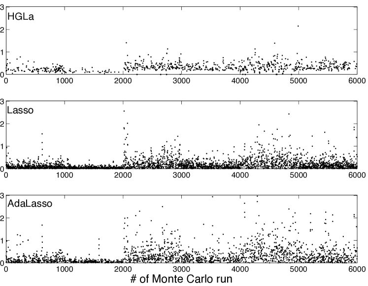
Figure 5: Comparison with AdaLasso (section 8.2). Euclidean norm of the estimates of the null components of $\theta$ returned by the three estimators (divided by the norm of the true $\theta$) as a function of the Monte Carlo runs performed in the 6 experiments. The values different from zero are displayed as points while no point is displayed if the obtained estimate is zero.

8.3 Real data

In order to test the algorithms on real data we have considered thermodynamic modeling of a small residential building. We placed sensors in two rooms of a small two-floor residential building of about 80 $\textrm{m}^{2}$ and 200 $\textrm{m}^{3}$; the sensors have been placed only on one floor (approximately 40 $\textrm{m}^{2}$ ) and their location is approximately shown in Figure 6. The larger room is the living room while the smaller is the kitchen.

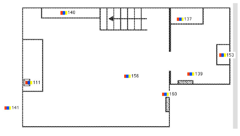
Figure 6: Nodes location: $8$ nodes each equipped with $3$ sensors: temperature, humidity and total radiation.

The experimental data was collected through a WSN made of 8 Tmote-Sky nodes produced by Moteiv Inc. Each Tmote-Sky is provided with a temperature sensor, a humidity sensor, and a total solar radiation photoreceptor (visible + infrared). The building was inhabited during the measurement period, which lasted for 8 days starting from February 24th, 2011; samples were taken every 5 minutes. The heating systems was controlled by a thermostat; the reference temperature was manually set every day depending upon occupancy and other needs.

The location of the sensors was as follows:

• Node $\#$1 (label 111 in Figure 6) was above a sideboard, about $1.8$ meters high, located close to thermoconvector.

• Node $\#$2 (label 137 in Figure 6) was above a cabinet (2.5 meters high).

• Node $\#$3 (label 139 in Figure 6) was above a cabinet (2.5 meters high).

• Node $\#$4 (label 140 in Figure 6) was placed on a bookshelf (1.5 meters high).

• Node $\#$5 (label 141 in Figure 6) was placed outside.

• Node $\#$6 (label 153 in Figure 6) was placed above the stove (2 meters high).

• Node $\#$7 (label 156 in Figure 6) was placed in the middle of the room, hanging from the ceiling (about 2 meters high).

• Node $\#$8 (label 160 in Figure 6) was placed above one radiator and was meant to provide a proxy of water temperature in the heating systems.

This gives a total of $24$ sensors (8 temperature + 8 humidity + 8 radiation signals). A preliminary inspection of the measured signals (see Figure 7) reveals the high level of collinearity which is well-known to complicate the estimation process in System Identification (Soderstrom and Stoica, 1989; Ljung, 1999; Box et al., ).

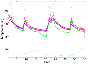
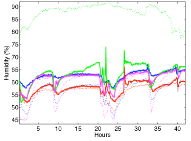
Figure 7: Measured temperatures (left) and humidity (right), first 40 hours.

We only consider Multiple Input-Single Output (MISO) models, with the temperature from each of the nodes as output ($y_{t}$) and all the other signals (7 temperatures, 8 humidities, 8 radiations) as inputs ($u^{i}_{t}$, $i=1,..,23$ ). We leave identification of a full Multiple Input-Multiple Output (MIMO) model for future investigation. We split the available data into $2$ parts; the first, composed of $N_{id}=700$ data points, is used for learning and validation and the second, composed of $N_{test}=1500$ data points, is used for test purposes. The notation $y^{id}$ identifies the training and validation data while $y^{test}$ identifies the test data. Note that $N_{id}=700$, with $5$ minute sampling times, corresponds to $\simeq 58\;hours$; this is a rather small time interval and, as such, models based on these data cannot capture seasonal variations. Consequently, in our experiments we assume a “stationary” environment and normalize the data so as to have zero mean and unit variance before identification is performed.

Our two main goals are as follows.

1. Provide meaningful models with as small data set as possible. This has clear advantages if identification is being performed for, e.g., certification purposes or as a preliminary step for deciding, having monitoring/control objectives in mind, how many sensors are needed and where these should be installed.

2. Provide sensor selection rules in order to reduce the number of sensors needed to effectively monitor the environment. A setup we have in mind is the following: one first deploys a large number of nodes, collects data and performs identification experiments. As an outcome, in addition to the models, we identify a subset of sensors that are sufficient to effectively monitor the environment; based on the measurements from this subset of sensors one can then reliably “predict” the evolution of temperature (and possibly humidity) across the building.

We envision that model predictive based methodologies, (see (Camacho and Bordons, 2004) and the recent papers (Yudong et al., 2010), (Pr vara et al., 2011), (Dong et al., 2008)), may be effective for these applications and, as such, we evaluate our models based on their ability to predict future data. The predictive power of the model is measured for $k$-step-ahead prediction on validation data, as:

$$COD_{k}:=1-{\frac{\sum_{t=k}^{N_{test}}(y^{test}_{t}-\hat{y}_{t|t-k})^{2}}{\sum_{t=k}^{N_{test}}(y^{test}_{t}-\bar{y}^{test})^{2}}}$$ (80)

where $\bar{y}^{test}:=\frac{1}{N_{test}}\sum_{t=1}^{N_{test}}y^{test}_{t}$.

We consider AutoRegressive models with eXogenous inputs (ARX) (Ljung, 1999; Soderstrom and Stoica, 1989; Box et al., ) of the form

$$y_{t}=\sum_{k=1}^{q}h_{k,1}y_{t-k}+\sum_{i=1}^{23}\sum_{k=1}^{q}h_{k,i+1}u_{t-k}^{i}+e_{t}\ .$$

This model is linear in the parameters ($h_{k,i}$, $k=1,..,q$, $i=1,..,24$) and as such falls within the general structure (1). Experiments with different lengths $q$ were investigated. We report only the results for $q=20$ which seemed to be the most reasonable choice for all methods. Note that, with reference to (15), here we have $p=24$ groups of $k_{i}=q=20$ parameters each, for a total of $480$ parameters.
We compare the performance of the following $2$ estimators:

• HGLc: the variant of HGLasso procedure defined at the end of Section 7. Identification data are split in a training and validation data set of equal size and the grid $C$ built around ${\hat{\kappa}}^{-1}$ used by the cross validation procedure to select $\gamma$ turns out to be $[25:25:1000]$.

• MKL (GLasso): the regularization parameter is estimated by cross validation using the same grid $C$ adopted for HGLc.

The $2$ estimators are compared using as performance indexes the $COD_{k}$ defined in equation (80). Sample trajectories of one-step-ahead prediction on both identification and test data are displayed in Figures 8 and 9 while $5$-hours ($=60$ steps) ahead prediction is shown in Figure 10.

The $COD_{k}$ up to $16$ hours ahead for ARX models are plotted in Figures 11 while Figure 12 shows the norm of the estimated impulse responses $h_{k,i}$, $i=1,..,24$.

It is clear that HGLc performs better than MKL in terms of prediction while achieving a higher level of sparsity. Note also that the higher sparsity achieved by HGLc results in a much more stable behavior in terms of multi-step prediction (see Figures 10 and 11). These results are in line with the theoretical findings in the paper as well as with the simulation results on synthetic data on Section 8.1.

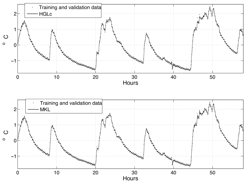
Figure 8: ARX model: training and validation data ($\cdot$) with output (solid line) estimated by HGLc (top) and MKL (bottom).

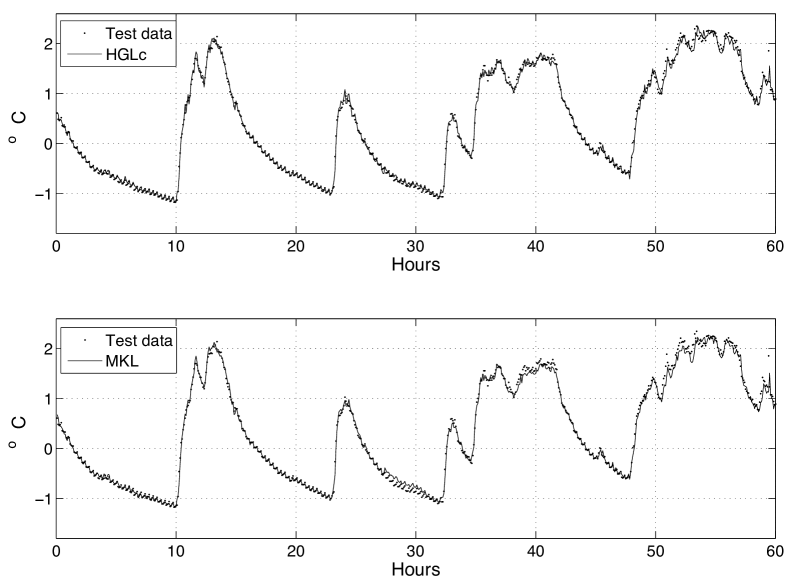
Figure 9: ARX model: test data ($\cdot$) and prediction (solid line) obtained by HGLc (top) and MKL (bottom).

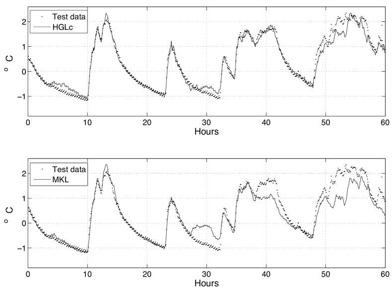
Figure 10: ARX model: test data ($\cdot$) and 5-hours ahead prediction (solid line) obtained by HGLc (top) and MKL (bottom).

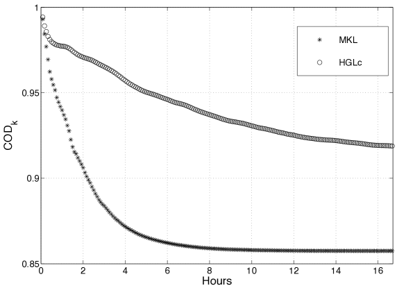
Figure 11: ARX model: coefficient of determination as a function of the prediction horizon (one step = 5 minutes) using HGLc (o) and MKL ($*$).

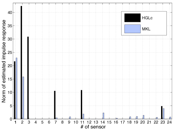
Figure 12: ARX model: norm of estimated impulse responses using HGLc and MKL.

9 Conclusions

We have presented a comparative study of two methods for sparse estimation: GLasso (equivalently, MKL) and the new HGLasso. They derive from the same Bayesian model, yet in a different way. The peculiarities of HGLasso can be summarized as follows:

• in comparison with GLasso, HGLasso derives from a marginalized joint density with the resulting estimator involving optimization of a non-convex objective;

• the non-convex nature allows HGLasso to achieve higher levels of sparsity than GLasso without introducing too much regularization in the estimation process;

• the MSE analysis reported in this paper reveals the superior performance of HGLasso also in the reconstruction of the parameter groups different from zero. Remarkably, our analysis elucidates this issue showing the robustness of the empirical Bayes procedure, based on marginal likelihood optimization, independently of the correctness of the priors entering the stochastic model underlying HGLasso. It also clarifies the asymptotic properties of ARD;

• the non-convex nature of HGLasso is not a limitation for its practical application. Indeed, the Bayesian Forward Selection used in HGLa provides a highly successful initialization procedure for the regularization parameter $\gamma$ ($\hat{\gamma}$), an initial estimate for $\lambda$ (using $\hat{\kappa}$), and an initial estimate of the non-zero groups ($I_{FS}$). This procedure requires only the solution of a one dimensional version of the basic problem (19).

Notice also that, being included in the framework of the Type II Bayesian estimators, many variations of HGLasso could be considered, adopting different prior models for $\lambda$. In this paper, the exponential prior has been used since the goal was the comparison of different estimators that can be derived from the same Bayesian model underlying GLasso. In this way, it has been also shown how, starting from the same stochastic framework, an estimator derived from a suitable posterior marginalization can have signi cant advantages over another one derived from posterior optimization.
All theoretical findings have been confirmed by experiments involving real and simulated data, also comparing the performance of the new approach with adaptive lasso. The aforementioned version of HGLasso has been able to promote sparsity correctly detecting a high percentage (in some experiments also equal to $99\%$) of the null blocks of the parameter vector and to provide accurate estimates of the non-null blocks.

10 Appendix

10.1 Proof of Proposition 5

Given $\gamma\geq 0$, the maximum a posteriori estimate for $(\phi,\lambda)$ given $y$ is obtained by solving the problem

$$\min_{\phi\in{\mathbb{R}}^{m},\lambda\in{\mathbb{R}}_{+}^{p}}\frac{(y-G\Lambda^{1/2}\phi)^{\top}(y-G\Lambda^{1/2}\phi)}{2\sigma^{2}}+\frac{\phi^{\top}\phi}{2}+\gamma\mathbf{1}^{\top}\lambda\ .$$ (81)

Minimizing first in $\phi$ allows us to write $\phi$ as the following function of $\lambda$:

$$\phi(\lambda):=(\sigma^{2}I+\Lambda^{1/2}G^{\top}G\Lambda^{1/2})^{-1}\Lambda^{1/2}G^{\top}y=\Lambda^{1/2}G^{\top}(\sigma^{2}I+K(\lambda))^{-1}y,$$ (82)

where the second expression follows from the Matrix Inversion Lemma. Substituting this back into (81) yields the optimization problem (34). Hence, if $\hat{\lambda}$ is as defined in (34), then (36) follows from (82).

Now, we show that the pair $(\hat{c},\hat{\lambda})$ described by (34) and (36) solves (31) for some value of $\gamma\geq 0$. For this, we need only show that the pair $(\hat{c},\hat{\lambda})$ is a local solution to (31) for some $\gamma\geq 0$. To this end, observe that (29) is coercive in $f$ (the objective goes to $\infty$ as the norm of $f$ goes to $\infty$) and $\lambda$ is constrained to stay in a compact set, so that a solution exists. Consequently a solution to (31) exists. Let $\gamma\geq 0$ be the Lagrange multiplier associated with a local solution $(c^{*},\lambda^{*})$ to (31) ($\gamma$ exists since the constraint is linear). We show that $(c^{*},\lambda^{*})=(\hat{c},\hat{\lambda})$. Since $\gamma$ is the Lagrange multiplier, $(c^{*},\lambda^{*})$ is a local solution to the problem

$$\min_{c\in{\mathbb{R}}^{n},\lambda\in{\mathbb{R}}_{p}^{+}}\frac{(y-K(\lambda)c)^{\top}(y-K(\lambda)c)}{\sigma^{2}}+c^{\top}K(\lambda)c+\gamma\mathbf{1}^{\top}\lambda\ .$$ (83)

As above, first optimize (83) in $c$ to obtain

$$c(\lambda)=(\sigma^{2}I+K(\lambda))^{-1}y.$$

Plugging this back into the objective in (83) gives the objective

$$y^{\top}(\sigma^{2}I+K(\lambda))^{-1}y+\gamma\mathbf{1}^{\top}\lambda$$

which establishes (34) and (35) for $(c^{*},\lambda^{*})$, and hence the pair $(c^{*},\lambda^{*})$ satisfies (34) and (36) by the first part of the proof and solves (31) by definition. Finally, (37) can be obtained reformulating the objective (81) in terms of $\theta=\Lambda^{1/2}\phi$ and $\lambda$ (in place of $\phi$ and $\lambda$), and then minimizing it first in $\lambda$.

10.2 Proof of Proposition 9

Under the simplifying assumption $G^{\top}G=nI$, one can use (9) to simplify the necessary conditions for optimality in (23). By (9), we have

$${G^{(i)}}^{\top}\Sigma_{y}(\lambda)^{-1}=\frac{1}{n\lambda_{i}+\sigma^{2}}{G^{(i)}}^{\top},$$

and so

$$\mbox{tr}\left(G^{(i)\top}\Sigma_{y}^{-1}G^{(i)}\right)=\frac{nk_{i}}{n\lambda_{i}+\sigma^{2}}\quad\mbox{and}\quad\|G^{(i)\top}\Sigma_{y}^{-1}y\|_{2}^{2}=\left(\frac{n}{n\lambda_{i}+\sigma^{2}}\right)^{2}\|\hat{\theta}_{LS}^{(i)}\|^{2}\ .$$

Inserting these expressions into (23) with $\mu_{i}=0$ yields a quadratic equation in $\lambda_{i}$ which always has two real solutions. One is always negative while the other, given by

$$\frac{1}{4\gamma}\left[\sqrt{k_{i}^{2}+8\gamma\|\hat{\theta}^{(i)}_{LS}\|^{2}}-\left(k_{i}+\frac{4\sigma^{2}\gamma}{n}\right)\right]$$

is non-negative provided

$$\frac{\|\hat{\theta}_{LS}^{(i)}\|^{2}}{k_{i}}\geq\frac{\sigma^{2}}{n}\left[1+\frac{2\gamma\sigma^{2}}{nk_{i}}\right]\ .$$ (84)

This concludes the proof of (46). The limiting behavior for $\gamma\rightarrow 0$ can be easily verified, yielding

$$\hat{\lambda}_{i}(0)={\rm max}\left(0,\frac{\|\hat{\theta}_{LS}^{(i)}\|^{2}}{k_{i}}-\frac{\sigma^{2}}{n}\right)\quad i=1,..,p.$$

Also note that $\hat{\theta}_{LS}^{(i)}=\frac{1}{n}\left(G^{(i)}\right)^{\top}y$ and $\left(G^{(i)}\right)^{\top}G^{(i)}=nI_{k_{i}}$ while $\left(G^{(i)}\right)^{\top}G^{(j)}=0$, $\forall j\neq i$. This implies that $\hat{\theta}_{LS}^{(i)}\sim{\cal N}({\bar{\theta}}^{(i)},\frac{\sigma^{2}}{n}I_{k_{i}})$. Therefore

$$\|\hat{\theta}_{LS}^{(i)}\|^{2}\frac{n}{\sigma^{2}}\sim\chi^{2}(d,\mu)\quad d=k_{i},\quad\mu=\|{\bar{\theta}}^{(i)}\|^{2}\frac{n}{\sigma^{2}}$$

This, together with (84), proves also (48).

10.3 Proof of Proposition 10

In the proof of Proposition 9 it was shown that $\|\hat{\theta}_{LS}^{(i)}\|^{2}\frac{n}{\sigma^{2}}$ follows a noncentral $\chi^{2}$ distribution with $k_{i}$ degrees of freedom and noncentrality parameter $\|\theta_{t}^{(i)}\|^{2}\frac{n}{\sigma^{2}}$. Hence, it is a simple calculation to show that

$${\mathbb{E}}[\hat{\lambda}^{*}_{i}\,|\,\theta={\bar{\theta}}]=\frac{\|{\bar{\theta}}^{(i)}\|^{2}}{k_{i}}\quad\mbox{Var}[\hat{\lambda}^{*}_{i}\,|\,\theta={\bar{\theta}}]=\frac{2\sigma^{4}}{k_{i}n^{2}}+\frac{4\|{\bar{\theta}}^{(i)}\|^{2}\sigma^{2}}{k_{i}^{2}n}\ .$$ (85)

By Corollary 8, the first of these equations shows that ${\mathbb{E}}[\hat{\lambda}_{i}^{*}\,|\,\theta={\bar{\theta}}]=\lambda_{i}^{opt}$. In addition, since $\mbox{Var}\{\hat{\lambda}^{*}_{i}\}$ goes to zero as $n\rightarrow\infty$, $\hat{\lambda}_{i}^{*}$ converges in mean square (and hence in probability) to $\lambda_{i}^{opt}$.

As for the analysis of $\hat{\lambda}_{i}(0)$, observe that

$${\mathbb{E}}[\hat{\lambda}_{i}(0)\,|\,\theta={\bar{\theta}}]={\mathbb{E}}[\hat{\lambda}^{*}_{i}\,|\,\theta={\bar{\theta}}]-\int_{0}^{k_{i}\frac{\sigma^{2}}{n}}\left(\frac{\|\hat{\theta}^{(i)}_{LS}\|^{2}}{k_{i}}-\frac{\sigma^{2}}{n}\right)dP({\|\hat{\theta}^{(i)}_{LS}\|^{2}}\,|\,\theta={\bar{\theta}})$$

where $dP({\|\hat{\theta}^{(i)}_{LS}\|^{2}}\,|\,\theta={\bar{\theta}})$ is the measure induced by $\|\hat{\theta}^{(i)}_{LS}\|^{2}$. The second term in this expression can be bounded by

$$-\int_{0}^{k_{i}\frac{\sigma^{2}}{n}}\left(\frac{\|\hat{\theta}^{(i)}_{LS}\|^{2}}{k_{i}}-\frac{\sigma^{2}}{n}\right)dP({\|\hat{\theta}^{(i)}_{LS}\|^{2}}\,|\,\theta={\bar{\theta}})\leq\frac{\sigma^{2}}{n}\int_{0}^{k_{i}\frac{\sigma^{2}}{n}}dP({\|\hat{\theta}^{(i)}_{LS}\|^{2}}\,|\,\theta={\bar{\theta}}),$$

where the last term on the right hand side goes to zero as $n\rightarrow\infty$. This proves that $\hat{\lambda}_{i}(0)$ is asymptotically unbiased. As for consistency, it is sufficient to observe that $\mbox{Var}[\hat{\lambda}_{i}(0)\,|\,\theta={\bar{\theta}}]\leq\mbox{Var}[\hat{\lambda}^{*}_{i}\,|\,\theta={\bar{\theta}}]$ since “saturation” reduces variance. Consequently, $\hat{\lambda}_{i}(0)$ converges in mean square to its mean, which asymptotically is $\lambda^{opt}_{i}$ as shown above. This concludes the proof.

10.4 Proof of Proposition 12

Following the same arguments as in the proof of Proposition 9, under the assumption $G^{\top}G=nI$ we have that

$$\|G^{(i)\top}\Sigma_{y}^{-1}y\|_{2}^{2}=\left(\frac{n}{n\lambda_{i}+\sigma^{2}}\right)^{2}\|\hat{\theta}_{LS}^{(i)}\|^{2}$$

Inserting this expression into (38) with $\mu_{i}=0$, one obtains a quadratic equation in $\lambda_{i}$ which has always two real solutions. One is always negative while the other, given by

$$\frac{\|\hat{\theta}_{LS}^{(i)}\|}{\sqrt{2\gamma}}-\frac{\sigma^{2}}{n}.$$

is non-negative provided

$$\|\hat{\theta}_{LS}^{(i)}\|^{2}\geq\frac{2\gamma\sigma^{4}}{n^{2}}\ .$$ (86)

This concludes the proof of (53).

The limiting behavior for $n\rightarrow\infty$ in equation (54) is easily verified with arguments similar to those in the proof of Proposition 10. As in the proof of Proposition 9, $\|\hat{\theta}_{LS}^{(i)}\|^{2}\frac{n}{\sigma^{2}}$ follows a noncentral $\chi^{2}(d,\mu)$ distribution with $d=k_{i}$ and $\mu=\|{\bar{\theta}}^{(i)}\|^{2}\frac{n}{\sigma^{2}}$, so that from (86) the probability of setting $\hat{\lambda}_{i}(\gamma)$ to zero is as given in (55).

10.5 Proof of Theorem 13

Recalling model (15), assume that $G^{\top}G/n$ is bounded and bounded away from zero in probability, so that there exist constants $\infty>c_{max}\geq c_{min}>0$ with

$$\lim_{n\rightarrow\infty}P[c_{min}I\leq G^{\top}G/n\leq c_{max}I]=1\;,$$ (87)

so as $n$ increases, the probability that a particular realization $G$ satisfies

$$c_{min}I\leq G^{\top}G/n\leq c_{max}I$$ (88)

increases to $1$. We now characterize the behavior of key matrices used in the analysis.

We first provide a technical lemma which will become useful in the sequel:

Lemma 16

Assume (88) holds; then the following conditions hold

1. Consider an arbitrary subset $I=[I(1),\dots,I(p_{I})]$ of size $p_{I}$ to be any subset of the indices $[1,\dots,p]$, so $p\leq p_{I}$ and define

   $$G^{(I)}=\begin{bmatrix}G^{({I(1)})}\dots G^{({I(p_{I})})}\end{bmatrix}\;,$$ (89)

   obtained by taking the subset of blocks of columns of $G$ indexed by $I$. Then

   $$c_{min}I\leq\frac{(G^{(I)})^{T}G^{(I)}}{n}\leq c_{max}I\;.$$ (90)

2. Let $I^{c}$ be the complementary set of $I$ in $[1,\dots,p]$, so that $I^{c}\cap I=\emptyset$ and $I\cup I^{c}=[1,\dots,p]$. The minimal angle $\theta_{min}$ between the spaces

   $${\cal G}^{I}:={col\,span}\{G^{(i)}/\sqrt{n},\;\;i\in I\}\quad{\rm and}\quad{\cal G}^{I^{c}}:={col\,span}\{G^{(j)}/\sqrt{n}:j\in I^{c}\}$$

   satisfies:

   $$\theta_{min}\geq{\rm acos}\left(\sqrt{1-\frac{c_{min}}{c_{max}}}\right)>0$$

Proof  Result (90) is a direct consequence of (Horn and Johnson, 1994, Corollary 3.1.3). As far as condition (ii) is concerned we can proceed as follows: let $U_{I}$ and $U_{I^{c}}$ be orthonormal matrices whose columns span ${\cal G}^{I}$ and ${\cal G}^{I^{c}}$, so that there exist matrices $T_{I}$ and $T_{I^{c}}$ so that

$$\begin{array}[]{c}G^{(I)}/\sqrt{n}=U_{I}T_{I}\\ G^{(I^{c})}/\sqrt{n}=U_{I^{c}}T_{I^{c}}\end{array}$$

where $G^{(I^{c})}$ is defined analogously to $G^{(I)}$. The minimal angle between ${\cal G}^{I}$ and ${\cal G}^{I^{c}}$ satisfies

$${\rm cos}(\theta_{min})=\left\|U_{I}^{\top}U_{I^{c}}\right\|.$$

Now observe that, up to a permutation of the columns which is irrelevant, $G/\sqrt{n}=[U_{I}T_{I}\;\;\;U_{I^{c}}T_{I^{c}}]$, so that

$$U_{I}^{\top}G/\sqrt{n}=[T_{I}\;\;\;U_{I}^{\top}U_{I^{c}}\ T_{I^{c}}]=[I\;\;\;U_{I}^{\top}U_{I^{c}}]\left[\begin{array}[]{cc}T_{I}&0\\ 0&T_{I^{c}}\end{array}\right].$$

Denoting with $\sigma_{min}(A)$ and $\sigma_{max}(A)$ the minimum and maximum singular values of a matrix $A$, it is a straightforward calculation to verify that the following chain of inequalities holds:

$$\begin{array}[]{rcl}c_{min}=\sigma_{min}(G^{\top}G/n)\leq\sigma^{2}_{min}\left(U_{I}^{\top}G/\sqrt{n}\right)&=&\sigma^{2}_{min}\left([I\;\;\;U_{I}^{\top}U_{I^{c}}]\left[\begin{array}[]{cc}T_{I}&0\\ 0&T_{I^{c}}\end{array}\right]\right)\\ &\leq&\sigma^{2}_{min}\left([I\;\;\;U_{I}^{\top}U_{I^{c}}]\right)\sigma^{2}_{max}\left(\left[\begin{array}[]{cc}T_{I}&0\\ 0&T_{I^{c}}\end{array}\right]\right)\\ &=&\sigma^{2}_{min}\left([I\;\;\;U_{I}^{\top}U_{I^{c}}]\right){\rm max}\left(\sigma^{2}_{max}(T_{I}),\sigma^{2}_{max}(T_{I^{c}})\right)\\ &\leq&\sigma^{2}_{min}\left([I\;\;\;U_{I}^{\top}U_{I^{c}}]\right)c_{max}.\end{array}$$

Observe now that $\sigma^{2}_{min}\left([I\;\;\;U_{I}^{\top}U_{I^{c}}]\right)=1-{\rm cos}^{2}(\theta_{min})$ so that

$$c_{min}\leq(1-{\rm cos}^{2}(\theta_{min}))c_{max}$$

and, therefore,

$${\rm cos}^{2}(\theta_{min})\leq 1-\frac{c_{min}}{c_{max}}$$

from which the thesis follow.  

Proof of Lemma 14: Let us consider the Singular Value Decomposition (SVD)

$$\frac{\sum_{j=1,j\neq i}^{p}G^{(j)}\left(G^{(j)}\right)^{\top}\lambda_{j}}{n}=PSP^{\top};$$ (91)

where, by the assumption (88), using $\frac{\sum_{j=1,j\neq i}^{p}G^{(j)}\left(G^{(j)}\right)^{\top}\lambda_{j}}{n}\geq\frac{\sum_{j=1,j\neq i,\lambda_{j}\neq 0}^{p}G^{(j)}\left(G^{(j)}\right)^{\top}}{n}{\rm min}\{\lambda_{j},j:\lambda_{j}\neq 0\}$ and lemma 16 the minimum singular value $\sigma_{min}(S)$ of $S$ in (91) satisfies

$$\sigma_{min}(S)\geq c_{min}{\rm min}\{\lambda_{j},j:\lambda_{j}\neq 0\}.$$ (92)

Then the SVD of $\Sigma_{\bar{v}}=\sum_{j=1,j\neq i}^{p}G^{(j)}\left(G^{(j)}\right)^{\top}\lambda_{j}+\sigma^{2}I$ satisfies

$$\Sigma_{\bar{v}}^{-1}=\left[\begin{array}[]{cc}P&P_{\perp}\end{array}\right]\left[\begin{array}[]{cc}(nS+\sigma^{2})^{-1}&0\\ 0&\sigma^{-2}I\end{array}\right]\left[\begin{array}[]{c}P^{\top}\\ P_{\perp}^{\top}\end{array}\right]$$

so that $\|\Sigma_{\bar{v}}^{-1}\|=\sigma^{-2}$.

Note now that

$$D_{n}^{(i)}=\left(U_{n}^{(i)}\right)^{\top}\frac{\Sigma_{\bar{v}}^{-1/2}G^{(i)}}{\sqrt{n}}V_{n}^{(i)}$$

and therefore, using Lemma 16,

$$\|D_{n}^{(i)}\|\leq\|\Sigma_{\bar{v}}^{-1}\|\sqrt{c_{max}}=\sigma^{-2}\sqrt{c_{max}}.$$

proving that $D^{(i)}_{n}$ is bounded. In addition, again using Lemma 16, condition (88) implies that $\forall a,b$ (of suitable dimensions) s.t. $\|a\|=\|b\|=1$, $a^{\top}\frac{P_{\perp}^{\top}G^{(i)}}{\sqrt{n}}b\geq k$, $k=\sqrt{1-{\rm cos}^{2}(\theta_{min})}\geq\frac{c_{min}}{c_{max}}>0$. This, using (62), guarantees that

$$\begin{array}[]{rcl}D_{n}^{(i)}&=&\left(U_{n}^{(i)}\right)^{\top}\frac{\Sigma_{\bar{v}}^{-1/2}G^{(i)}}{\sqrt{n}}V_{n}^{(i)}=\left(U_{n}^{(i)}\right)^{\top}\left(P(nS+\sigma^{2})^{-1/2}P^{\top}+P_{\perp}\sigma^{-1}P_{\perp}^{\top}\right)\frac{G^{(i)}}{\sqrt{n}}\\ &\geq&\left(U_{n}^{(i)}\right)^{\top}\left(P_{\perp}\sigma^{-1}P_{\perp}^{\top}\right)\frac{G^{(i)}}{\sqrt{n}}\\ &\geq&k\sigma^{-1}I\end{array}$$

and therefore $D^{(i)}_{n}$ is bounded away from zero. It is then a matter of simple calculations to show that with the definitions (64) then (61) can be rewritten in the equivalent form (63). ${\square}$

Lemma 17

Assume, w.l.o.g., that the blocks of $\theta$ have been reordered so that $\|\bar{\theta}^{(j)}\|\neq 0$, $j=1,..,k$ and $\|\bar{\theta}^{(j)}\|=0$, $j=k+1,..,m$ and that the spectrum of $G^{\top}G/n$ is bounded and bounded away from zero in probability, so that

$${\rm lim}_{n\rightarrow\infty}P[c_{max}I\geq G^{\top}G/n\geq c_{min}I]=1.$$ (93)

Denote

$$\begin{array}[]{c}I_{1}:=\{j\in[1,k],\;j\neq i\}\\ I_{0}:=\{j\in[k+1,p],\;j\neq i\}\end{array}$$

and assume also that the numbers $\lambda_{j}^{n}$, which are here allowed to depend on $n$, are bounded and satisfy:

$$\begin{array}[]{c}\displaystyle{\mathop{\rm lim}_{n\rightarrow\infty}}\;f_{n}=+\infty\quad{\rm where}\quad f_{n}:=\displaystyle{\mathop{\rm min}_{j\in I_{1}}}\;n\lambda_{j}^{n}\end{array}$$ (94)

Then, conditioned on $\theta$, $\epsilon_{n}^{(i)}$ in (64) and (63) can be decomposed as

$$\epsilon_{n}^{(i)}=m_{\epsilon_{n}}(\theta)+v_{\epsilon_{n}}.$$ (95)

The following conditions hold:

$${\mathbb{E}}_{v}\left[\epsilon_{n}^{(i)}\right]=m_{\epsilon_{n}}(\theta)=O_{P}\left(\frac{1}{\sqrt{f_{n}}}\right)\quad\quad v_{\epsilon_{n}}=O_{P}\left(\frac{1}{\sqrt{n}}\right)$$ (96)

so that $\epsilon_{n}^{(i)}|\theta$ converges to zero in probability (as $n\rightarrow\infty$). In addition

$${Var}_{v}\{\epsilon_{n}^{(i)}\}={\mathbb{E}}_{v}\left[v_{\epsilon_{n}}v_{\epsilon_{n}}^{\top}\right]=O_{P}\left(\frac{1}{{n}}\right).$$ (97)

If in addition

$$n^{1/2}\frac{\left(G^{(i)}\right)^{\top}G^{(j)}}{n}=O_{P}(1)\;\;;\;j=1,..,k\;\;j\neq i$$ (98)

then

$$m_{\epsilon_{n}}(\theta)=O_{P}\left(\frac{1}{\sqrt{nf_{n}}}\right)$$ (99)

Proof  Consider the Singular Value Decomposition

$$\bar{P}_{1}\bar{S}_{1}\bar{P}_{1}^{\top}:=\frac{1}{n}\sum_{j\in I_{1}}G^{(j)}\left(G^{(j)}\right)^{\top}\lambda_{j}^{n}.$$ (100)

Using (94), there exist $\bar{n}$ so that, $\forall\;n>\bar{n}$ we have $0<\lambda_{j}^{n}\leq M<\infty$, $j\in I_{1}$. Otherwise, we could find a subsequence $n_{k}$ so that $\lambda_{j}^{n_{k}}=0$ and hence $n_{k}\lambda_{j}^{n_{k}}=0$, contradicting (94). Therefore, the matrix $\bar{P}_{1}$ in (100) is an orthonormal basis for the space ${\cal G}_{1}:={col\,span}\{G^{(j)}/\sqrt{n}:j\in I_{1}\}$. Let also $T_{j}$ be such that $G^{(j)}/\sqrt{n}=\bar{P}_{1}T_{j}$, $j\in I_{1}$. Note that by assumption (87) and lemma 16

$$\|T_{j}\|=O_{P}(1)\quad\forall\,j\in I_{1}.$$ (101)

Consider now the Singular Value Decomposition

$$\begin{array}[]{rcccc}\left[\begin{array}[]{cc}P_{1}&P_{0}\end{array}\right]\left[\begin{array}[]{cc}S_{1}&0\\ 0&S_{0}\end{array}\right]\left[\begin{array}[]{c}P_{1}^{\top}\\ P_{0}^{\top}\end{array}\right]&:=&\underbrace{\frac{1}{n}\sum_{j\in I_{1}}G^{(j)}\left(G^{(j)}\right)^{\top}\lambda_{j}^{n}}&+&\underbrace{\frac{1}{n}\sum_{j\in I_{0}}G^{(j)}\left(G^{(j)}\right)^{\top}\lambda_{j}^{n}}\\ &=&\bar{P}_{1}\bar{S}_{1}\bar{P}_{1}^{\top}&+&\Delta.\end{array}$$ (102)

For future reference note that $\exists T_{\bar{P}_{1}}\;:\;\bar{P}_{1}=\left[\begin{array}[]{cc}P_{1}&P_{0}\end{array}\right]T_{\bar{P}_{1}}$. Now, from (62) we have that

$$\frac{\Sigma_{\bar{v}}^{-1}G^{(i)}}{\sqrt{n}}V_{n}^{(i)}\left(D_{n}^{(i)}\right)^{-1}=\Sigma_{\bar{v}}^{-1/2}U_{n}^{(i)}.$$ (103)

Using (103) and defining

$$P:=\left[\begin{array}[]{cc}P_{1}&P_{0}\end{array}\right]\quad S:=\left[\begin{array}[]{cc}S_{1}&0\\ 0&S_{0}\end{array}\right],$$

equation (64) can be rewritten as:

$$\begin{array}[]{rcl}\epsilon_{n}^{(i)}&=&\left(U_{n}^{(i)}\right)^{\top}\frac{\Sigma_{\bar{v}}^{-1/2}\bar{v}}{\sqrt{n}}\\ &=&\left(D_{n}^{(i)}\right)^{-1}\left(V_{n}^{(i)}\right)^{\top}\frac{\left(G^{(i)}\right)^{\top}}{\sqrt{n}}\Sigma_{\bar{v}}^{-1}\frac{\bar{v}}{\sqrt{n}}\\ &=&\left(D_{n}^{(i)}\right)^{-1}\left(V_{n}^{(i)}\right)^{\top}\frac{\left(G^{(i)}\right)^{\top}}{\sqrt{n}}\left[\begin{array}[]{cc}P&P_{\perp}\end{array}\right]\left[\begin{array}[]{cc}(nS+\sigma^{2}I)^{-1}&0\\ 0&\sigma^{-2}I\end{array}\right]\left[\begin{array}[]{c}P^{\top}\\ P_{\perp}^{\top}\end{array}\right]\frac{\bar{v}}{\sqrt{n}}\\ &=&\left(D_{n}^{(i)}\right)^{-1}\left(V_{n}^{(i)}\right)^{\top}\frac{\left(G^{(i)}\right)^{\top}}{\sqrt{n}}\left[\begin{array}[]{cc}P&P_{\perp}\end{array}\right]\left[\begin{array}[]{cc}(nS+\sigma^{2}I)^{-1}&0\\ 0&\sigma^{-2}I\end{array}\right]\left[\begin{array}[]{c}P^{\top}\\ P_{\perp}^{\top}\end{array}\right]\left[\sum_{j\in I_{1}}\frac{G^{(j)}}{\sqrt{n}}\theta^{(j)}+\frac{v}{\sqrt{n}}\right]\\ &=&\underbrace{\left(D_{n}^{(i)}\right)^{-1}\left(V_{n}^{(i)}\right)^{\top}\frac{\left(G^{(i)}\right)^{\top}}{\sqrt{n}}P(nS+\sigma^{2}I)^{-1}\left[\begin{array}[]{c}P_{1}^{\top}P_{1}\\ P_{0}^{\top}P_{1}\end{array}\right]\sum_{j\in I_{1}}T^{(j)}\theta^{(j)}}_{m_{\epsilon_{n}}(\theta)}+\\ &&+\underbrace{\left(D_{n}^{(i)}\right)^{-1}\left(V_{n}^{(i)}\right)^{\top}\frac{\left(G^{(i)}\right)^{\top}}{\sqrt{n}}\left[\begin{array}[]{cc}P&P_{\perp}\end{array}\right]\left[\begin{array}[]{cc}(nS+\sigma^{2}I)^{-1}&0\\ 0&\sigma^{-2}I\end{array}\right]\frac{v_{\bar{p}}}{\sqrt{n}}}_{v_{\epsilon_{n}}}\end{array}$$

where the last equation defines $m_{\epsilon_{n}}(\theta)$ and $v_{\epsilon_{n}}$, the noise

$$v_{\bar{P}}:=\left[\begin{array}[]{c}P^{\top}\\ P_{\perp}^{\top}\end{array}\right]v$$

is still a zero mean Gaussian noise with variance $\sigma^{2}I$ and $\frac{G^{(j)}}{\sqrt{n}}=P_{1}T^{(j)}$ provided $j\neq i$. Note that $m_{\epsilon_{n}}$ does not depend on $v$ and that ${\mathbb{E}}_{v}v_{\epsilon_{n}}=0$. Therefore $m_{\epsilon_{n}}(\theta)$ is the mean (when only noise $v$ is averaged out) of $\epsilon_{n}$. As far as the asymptotic behavior of $m_{\epsilon_{n}}(\theta)$ is concerned, it is convenient to preliminary observe that

$$(nS+\sigma^{2}I)^{-1}\left[\begin{array}[]{c}P_{1}^{\top}\bar{P}_{1}\\ P_{0}^{\top}\bar{P}_{1}\end{array}\right]=\left[\begin{array}[]{c}(nS_{1}+\sigma^{2}I)^{-1}P_{1}^{\top}\bar{P}_{1}\\ (nS_{0}+\sigma^{2}I)^{-1}P_{0}^{\top}\bar{P}_{1}\end{array}\right]$$

and that the second term on the right hand side can be rewritten as

$$(nS_{0}+\sigma^{2}I)^{-1}P_{0}^{\top}\bar{P}_{1}=\left[\begin{array}[]{c}(n[S_{0}]_{1,1}+\sigma^{2}I)^{-1}P_{0,1}^{\top}\bar{P}_{1}\\ (n[S_{0}]_{22}+\sigma^{2}I)^{-1}P_{0,2}^{\top}\bar{P}_{1}\\ \vdots\\ (n[S_{0}]_{m-k,m-k}+\sigma^{2}I)^{-1}P_{0,m-k}^{\top}\bar{P}_{1}\end{array}\right]$$ (104)

where $[S_{0}]_{ii}$ is the $i-th$ diagonal element of $S_{0}$ and $P_{0,i}$ if the $i-th$ column of $P_{0}$. Now, using equation (102) one obtains that

$$\begin{array}[]{rcl}n[S_{0}]_{ii}=P_{0,i}^{\top}PnSP^{\top}P_{0,i}&=&P_{0,i}^{\top}\left(\bar{P}_{1}n\bar{S}_{1}\bar{P}_{1}^{\top}+n\Delta\right)P_{0,i}\\ &\geq&P_{0,i}^{\top}\bar{P}_{1}n\bar{S}_{1}\bar{P}_{1}^{\top}P_{0,i}\\ &\geq&\sigma_{min}(n\bar{S}_{1})P_{0,i}^{\top}\bar{P}_{1}\bar{P}_{1}^{\top}P_{0,i}\\ &=&\sigma_{min}(n\bar{S}_{1})\|P_{0,i}^{\top}\bar{P}_{1}\|^{2}.\end{array}$$

With an argument similar to that used in (92), also

$$\sigma_{min}(n\bar{S}_{1})\geq c_{min}{\rm min}\{n\lambda_{j}^{n},\;j\in I_{1}\}=c_{min}f_{n}$$ (105)

holds true; denoting $\|P_{0,i}^{\top}\bar{P}_{1}\|=g_{n}$, the generic term on the right hand side of (104) satisfies

$$\begin{array}[]{rcl}\|(n[S_{0}]_{ii}+\sigma^{2}I)^{-1}P_{0,i}^{\top}\bar{P}_{1}\|&\leq&\frac{\|P_{0,i}^{\top}\bar{P}_{1}\|}{n\sigma_{min}(\bar{S}_{1})\|P_{0,i}^{\top}\bar{P}_{1}\|^{2}+\sigma^{2}}\\ &\leq&k\;{\rm min}(g_{n},(f_{n}g_{n})^{-1})\\ &=&\frac{k}{\sqrt{f_{n}}}{\rm min}(\sqrt{f_{n}}g_{n},(\sqrt{f_{n}}g_{n})^{-1})\\ &\leq&\frac{k}{\sqrt{f_{n}}}\end{array}$$ (106)

for some positive constant $k$. Now, using lemma 14, $D_{n}^{(i)}$ is bounded and bounded away from zero in probability, so that $\|D_{n}^{(i)}\|=O_{P}(1)$ and $\|\left(D_{n}^{(i)}\right)^{-1}\|=O_{P}(1)$. In addition $V_{n}^{(i)}$ is an orthonormal matrix and $\|\frac{G^{(i)}}{\sqrt{n}}\|=O_{P}(1)$. Last, using (105) and (93), we have $\|(nS_{1}+\sigma^{2})^{-1}\|=O_{P}(1/n)$. Combining these conditions with (101) and (106) we obtain the first of (96). As far as the asymptotics on $v_{\epsilon_{n}}$ are concerned, it suffices to observe that

$$w_{n}^{\top}v_{\bar{P}}/\sqrt{n}=O_{P}(1/\sqrt{n})\;\;{\rm if}:\;\|w_{n}\|=O_{P}(1).$$

The variance (w.r.t. noise $v$) ${Var}_{v}\{{\epsilon_{n}}\}={\mathbb{E}}_{v}\left[v_{\epsilon_{n}}v_{\epsilon_{n}}^{\top}\right]$ satisfies

$${Var}_{v}\{{\epsilon_{n}}\}=\frac{\sigma^{2}}{n}\left(U_{n}^{(i)}\right)^{\top}\Sigma_{v}^{-1}\left(U_{n}^{(i)}\right)$$

so that, using the condition $\|\Sigma_{\bar{v}}^{-1}\|=\sigma^{-2}$ derived in Lemma 14, and the fact that $U_{n}^{(i)}$ has orthonormal columns, the condition ${Var}_{v}\{{\epsilon_{n}}\}=O_{P}\left(\frac{1}{n}\right)$ in (97) follows immediately.

If in addition (98) holds then (101) becomes

$$\|T_{j}\|=O_{P}(1/\sqrt{n})\quad j=1,...,k;\;\;\;j\neq k$$

so that and extra $\sqrt{n}$ appears at the denominator in the expression of $m_{\epsilon}(\theta)$ yielding (99). This concludes the proof.  

Our next results will focus on the estimator (56). We will show that when the hypotheses of Lemma 14 hold, estimator (19) satisfies the key hypothesis of Lemma 17. We first take a close look at the objective (19).

Lemma 18

Take objective (19) divided by $n$:

$$g_{n}(\lambda)=\log\sigma^{2}+ \underbrace{\frac{1}{2n}\log\det(\sigma^{-2}\Sigma_{y}(\lambda))}_{S_{1}}+\underbrace{\frac{1}{2n}\sum_{j\in I_{1}}\frac{\|\hat{\theta}^{(j)}(\lambda)\|^{2}}{k_{j}\lambda_{j}}}_{S_{2}}+\underbrace{\frac{1}{2n}\sum_{j\in I_{0}}\frac{\|\hat{\theta}^{(j)}(\lambda)\|^{2}}{k_{j}\lambda_{j}}}_{S_{3}}$$ (107)

$$+\underbrace{\frac{1}{n}\gamma\|\lambda\|_{1}}_{S_{4}}+\underbrace{\frac{1}{2n\sigma^{2}}\|y-\sum_{j}G^{j}\hat{\theta}^{(j)}(\lambda)\|^{2}}_{S_{5}}\;,$$

where $\hat{\theta}(\lambda)=\Lambda G^{T}\Sigma_{y}^{-1}y$ (see (21)), $k_{j}$ is the size of the $j$th block, and dependence on $n$ has been suppressed. For any minimizing sequence $\lambda^{n}$, we have the following results:

1. $\hat{\theta}_{n}\rightarrow_{p}\bar{\theta}$.

2. $S_{1},S_{2},S_{3},S_{4}\rightarrow_{p}0$.

3. $S_{5}\rightarrow_{p}\frac{1}{2}$.

4. $n\lambda_{j}^{n}\rightarrow_{p}\infty$ for all $j\in I_{1}$.

Proof  First, note that $0\leq S_{i}$ for $i\in\{1,2,3,4\}$. Next,

$$S_{5} =\frac{1}{2n\sigma^{2}}\|y-\sum_{j}G^{j}\bar{\theta}^{(j)}(\lambda)+\sum_{j}G^{j}\left(\bar{\theta}^{(j)}(\lambda)-\hat{\theta}^{(j)}(\lambda)\right)\|^{2}$$ (108)

$$=\frac{1}{2n\sigma^{2}}\|\nu+\sum_{j}G^{j}\left(\bar{\theta}^{(j)}(\lambda)-\hat{\theta}^{(j)}(\lambda)\right)\|^{2}$$

$$=\frac{1}{2n\sigma^{2}}\|\nu\|^{2}+\frac{1}{2n\sigma^{2}}\nu^{T}\sum_{j}G^{j}\left(\bar{\theta}^{(j)}(\lambda)-\hat{\theta}^{(j)}(\lambda)\right)+\frac{1}{2n\sigma^{2}}\|\sum_{j}G^{j}\left(\bar{\theta}^{(j)}(\lambda)-\hat{\theta}^{(j)}(\lambda)\right)\|^{2}.$$

The first term converges in probability to $\frac{1}{2}$. Since $\nu$ is independent of all $G^{j}$, the middle term converges in probability to $0$. The third term is the bias incurred unless $\hat{\theta}=\bar{\theta}$. These facts imply that, $\forall\epsilon>0$,

$$\lim_{n\rightarrow\infty}P\left[S_{5}(\lambda(n))>\frac{1}{2}-\epsilon\right]=1\;.$$ (109)

Next, consider the particular sequence $\bar{\lambda}_{j}^{n}=\frac{\|\bar{\theta}_{j}\|^{2}}{k_{j}}$. For this sequence, it is immediately clear that $S_{i}\rightarrow_{p}0$ for $i\in\{2,3,4\}$. To show $S_{1}\rightarrow_{p}0$, note that $\sum\lambda_{i}G_{i}G_{i}^{T}\leq\max\{\lambda_{i}\}\sum G_{i}G_{i}^{T}$, and that the nonzero eigenvalues of $GG^{T}$ are the same as those of $G^{T}G$. Therefore, we have

$$S_{1}\leq\frac{1}{2n}\sum_{i=1}^{m}\log(1+n\sigma^{-2}\max\{\lambda\}c_{max})=O_{P}\left(\frac{\log(n)}{n}\right)\rightarrow_{p}0\;.$$

Finally $S_{5}\rightarrow_{p}\frac{1}{2}$ by (108), so in fact, $\forall\epsilon>0$,

$$\lim_{n\rightarrow\infty}P\left[\left|g_{n}(\bar{\lambda}(n))-\frac{1}{2}-\log(\sigma^{2})\right|<\epsilon\right]=1\;.$$ (110)

Since (110) holds for the deterministic sequence $\bar{\lambda}_{n}$, any minimizing sequence $\hat{\lambda}_{n}$ must satisfy, $\forall\epsilon>0$,

$$\lim_{n\rightarrow\infty}P\left[g_{n}(\hat{\lambda}(n))<\frac{1}{2}+\log(\sigma^{2})+\epsilon\right]=1\;.$$ (111)

which, together with (109), implies (110)

Claims $1,2,3$ follow immediately. To prove claim 4, suppose that for a particular minimizing sequence $\check{\lambda}(n)$, we have $n\check{\lambda}_{j}^{n}\not\rightarrow_{p}\infty$ for $j\in I_{1}$. We can therefore find a subsequence where $n\check{\lambda}_{j}^{n}\leq K$, and since $S_{2}(\check{\lambda}(n))\rightarrow_{p}0$, we must have $\|\check{\theta}^{(j)}(\check{\lambda})\|\rightarrow_{p}0.$ But then there is a nonzero bias term in (108), since in particular $\bar{\theta}^{(j)}(\lambda)-\hat{\theta}^{(j)}(\lambda)=\bar{\theta}^{(j)}(\lambda)\neq 0$, which contradicts the fact that $\check{\lambda}(n)$ was a minimizing sequence.  

Before we proceed, we review a useful characterization of convergence. While it can be stated for many types of convergence, we present it specifically for convergence in probability, since this is the version we will use.

Remark 19

$a^{n}$ converges in probability to $a$ (written $a^{n}\rightarrow_{p}a)$ if and only if every subsequence $a^{n(j)}$ of $a^{n}$ has a further subsequence $a^{n(j(k))}$ with $a^{n(j(k))}\rightarrow_{p}a$.

Proof  If $a^{n}\rightarrow_{p}a$, this means that for any $\epsilon>0$, $\delta>0$ there exists some $n_{\epsilon,\delta}$ such that for all $n\geq n_{\epsilon,\delta}$, we have $P(|a^{n}-a|>\epsilon)\leq\delta$. Clearly, if $a^{n}\rightarrow_{p}a$, then $a^{n(j)}\rightarrow_{p}a$ for every subsequence $a^{n(j)}$ of $a^{n}$. We prove the other direction by contrapositive.

Assume that $a^{n}\not\rightarrow_{p}a$. That means precisely that there exist some $\epsilon>0,\delta>0$ and a subsequence $a^{n(j)}$ so that $P(|a-a^{n(j)}|>\epsilon)\geq\delta$. Therefore the subsequence $a^{n(j)}$ cannot have further subsequences that converge to $a$ in probability, since every term of $a^{n(j)}$ stays $\epsilon$-far away from $a$ with positive probability $\delta$.  
Remark 19 plays a major role in the next lemma from which Theorem 13 immediately comes.

Lemma 20

Let $\lambda_{1}$ be arbitrary and consider the estimator (56) along $\lambda_{1}$ that, in view of (63), is given by:

$$\hat{\lambda}_{1}^{n}=\arg\min_{{\lambda}\in{\mathbb{R}}_{+}}\frac{1}{2}\sum_{k=1}^{k_{1}}\left[\frac{\eta_{k,n}^{2}+v_{k,n}}{\lambda+w_{k,n}}+\log(\lambda+w_{k,n})\right]+\gamma\lambda\;,$$ (112)

where $w_{k,n}:=1/(n(d^{(1)}_{k,n})^{2})$ and $v_{k,n}=2\epsilon_{k,n}^{(1)}d_{k,n}^{(1)}+(\epsilon_{k,n}^{(1)})^{2}$. Suppose that the hypotheses of Lemma 14 hold, so that $w_{k,n}\rightarrow 0$. Then by Lemma 18 we know Lemma 17 applies, so that $v_{k,n}\rightarrow_{p}0$. Let

$$\bar{\lambda}_{1}^{\gamma}:=\frac{-k_{1}+\sqrt{k_{1}^{2}+8\gamma\|\theta^{(1)}\|^{2}}}{4\gamma}\;,\quad\bar{\lambda}_{1}=\frac{\|\theta^{(1)}\|^{2}}{k_{1}}\;.$$

We have the following results:

1. $\bar{\lambda}_{1}^{\gamma}\leq\bar{\lambda}_{1}$ for all $\gamma>0$, and $\lim_{\gamma\rightarrow 0^{+}}\bar{\lambda}_{1}^{\gamma}=\bar{\lambda}_{1}$ .

2. If $\|\theta^{(1)}\|>0$ and $\gamma>0$, we have $\hat{\lambda}_{1}^{n}\longrightarrow_{p}\bar{\lambda}_{1}^{\gamma}$ .

3. If $\|\theta^{(1)}\|>0$ and $\gamma=0$, we have $\hat{\lambda}_{1}^{n}\longrightarrow_{p}\bar{\lambda}_{1}$ .

4. if $\theta^{(1)}=0$, we have $\hat{\lambda}_{1}^{\gamma}\longrightarrow_{p}0$ for any value $\gamma\geq 0$.

Proof 

1. The reader can quickly check that $\frac{d}{d\gamma}\bar{\lambda}_{1}^{\gamma}<0$, so $\bar{\lambda}_{1}^{\gamma}$ is decreasing in $\gamma$. The limit calculation follows immediately from L’Hopital’s rule it is clear that $\lim_{\gamma\rightarrow 0^{+}}\lambda_{1}^{\gamma}=\bar{\lambda}_{1}$.

2. We use the convergence characterization given in Remark 19. Pick any subsequence $\hat{\lambda}^{n(j)}_{1}$ of $\hat{\lambda}^{n}_{1}$. Since $\{V_{n(j)}\}$ is bounded, by Bolzano-Weierstrass it must have a convergent subsequence $V_{n(j(k))}\rightarrow V$, where $V$ satisfies $V^{T}V=I$ by continuity of the $2$-norm. The first order optimality conditions for $\hat{\lambda}_{1}^{n}>0$ are given by

   $$0=f_{1}(\lambda,w,v,\eta)=\frac{1}{2}\sum_{k=1}^{k_{1}}\frac{-\eta_{k}^{2}-v_{k}}{(\lambda+w_{k})^{2}}+\frac{1}{\lambda+w_{k}}+\gamma\;,$$ (113)

   and we have $f_{1}(\lambda,0,0,V^{T}\theta^{(1)})=0$ if and only if $\lambda=\bar{\lambda}_{1}^{\gamma}$. Taking the derivative we find

   $$\frac{d}{d\lambda}f_{1}(\lambda,0,0,V^{T}\theta^{(1)})=\frac{\|\theta^{(1)}\|^{2}}{\lambda^{3}}-\frac{k_{1}}{2\lambda^{2}}\;,$$

   which is nonzero at $\lambda_{1}^{\gamma}$ for any $\gamma$, since the only zero is at $2\frac{\|\theta^{(1)}\|^{2}}{k_{1}}=2\bar{\lambda}_{1}\geq 2\bar{\lambda}_{1}^{\gamma}$.

   Applying the Implicit Function Theorem to $f$ at $\left(\lambda_{1}^{\gamma},0,0,V^{\top}{\bar{\theta}}^{(1)}\right)$ yields the existence of neighborhoods $\mathcal{U}$ of $(0,0,V^{\top}{\bar{\theta}}^{(1)})$ and $\mathcal{W}$ of $\lambda_{1}^{\gamma}$ such that

   $$f(\phi(w,v,\eta),w,v,\eta)=0\qquad\forall\,(w,v,\eta)\in\mathcal{U}\ .$$

   In particular, $\phi(0,0,V^{\top}{\bar{\theta}}^{(1)})=\lambda_{1}^{\gamma}$. Since $(w_{n(j(k))},v_{n(j(k))},\eta_{n(j(k))})\rightarrow_{p}(0,0,V^{\top}{\bar{\theta}}^{(1)})$, we have that for any $\delta>0$ there exist some $k_{\delta}$ so that for all $n(j(k))>n(j(k_{\delta}))$ we have $P((w_{n(j(k)},v_{n(j(k))},\eta_{n(j(k))})\not\in\mathcal{U})\leq\delta$. For anything in $\mathcal{U}$, by continuity of $\phi$ we have

   $$\hat{\lambda}^{n(j(k))}_{1}=\phi(w_{n(j(k))},v_{n(j(k))},\eta_{n(j(k))})\rightarrow_{p}\phi(0,0,V^{\top}{\bar{\theta}}^{(1)})=\lambda_{1}^{\gamma}\;.$$

   These two facts imply that $\hat{\lambda}^{n(j(k))}_{1}\rightarrow_{p}\lambda_{1}^{\gamma}$. We have shown that every subsequence $\hat{\lambda}^{n(j)}_{1}$ has a further subsequence $\hat{\lambda}^{n(j(k))}_{1}\rightarrow_{p}\lambda_{1}^{\gamma}$, and therefore $\hat{\lambda}^{n}_{1}\rightarrow_{p}\lambda_{1}^{\gamma}$ by Remark 19.

3. In this case, the only zero of (113) with $\gamma=0$ is found at $\bar{\lambda}_{1}$, and the derivative of the optimality conditions is nonzero at this estimate, by the computations already given. The result follows by the implicit function theorem and subsequence argument, just as in the previous case.

4. Rewriting the derivative (113)

   $$\frac{1}{2}\sum_{k=1}^{k_{1}}\frac{\lambda-v_{k}-\eta_{k}^{2}+w_{k}}{(\lambda+w_{k})^{2}}+\gamma\;,$$

   we observe that for any positive lambda, the probability that the derivative is positive tends to one. Therefore the minimizer $\lambda_{1}^{\gamma}$ converges to $0$ in probability, regardless of the value of $\gamma$.

References

- Aravkin et al. [2012] A. Aravkin, J. Burke, A. Chiuso, and G. Pillonetto. On the estimation of hyperparameters for empirical bayes estimators: Maximum marginal likelihood vs minimum MSE. In Proc. IFAC Symposium on System Identification (SysId 2012), 2012.
- Bach et al. [2004] F. Bach, G. Lanckriet, and M. Jordan. Multiple kernel learning, conic duality, and the smo algorithm. In Proceedings of the 21st International Conference on Machine Learning, page 41 48, 2004.
- Bach [2008] F.R. Bach. Consistency of the group lasso and multiple kernel learning. Journal of Machine Learning Research, 9:1179–1225, 2008.
- Bauer [2005] D. Bauer. Asymptotic properties of subspace estimators. Automatica, 41:359–376, 2005.
- Berger [1985] J.O. Berger. Statistical Decision Theory and Bayesian Analysis. Springer Series in Statistics. Springer, second edition, 1985.
- [6] G. Box, G.M. Jenkins, and G. Reinsel. Time Series Analysis: Forecasting & Control. 3rd edition.
- Breiman [1995] L. Breiman. Better subset regression using the nonnegative garrote. Technometrics, 37:373–384, November 1995. ISSN 0040-1706. doi: 10.2307/1269730. URL http://portal.acm.org/citation.cfm?id=219631.219633.
- Camacho and Bordons [2004] E.F. Camacho and C. Bordons. Model Predictive Control. Advanced Textbooks in Control and Signal Processing. Springer Verlag, 2004.
- Candes and Tao [2007] E. Candes and T. Tao. The Dantzig selector: statistical estimation when is much larger than . Annals of Statistics, 35:2313–2351, 2007.
- Chatelin [1983] F. Chatelin. Spectral approximation of linear operators. Academic Press, NewYork, 1983.
- Chen et al. [2011] T. Chen, H. Ohlsson, and L. Ljung. On the estimation of transfer functions, regularization and gaussian processes - revisited. In IFAC World Congress 2011, Milano, 2011.
- Chiuso and Pillonetto [2010a] A. Chiuso and G. Pillonetto. Nonparametric sparse estimators for identification of large scale linear systems. In Proceedings of IEEE Conf. on Dec. and Control, Atlanta, 2010a.
- Chiuso and Pillonetto [2010b] A. Chiuso and G. Pillonetto. Learning sparse dynamic linear systems using stable spline kernels and exponential hyperpriors. In Proceedings of Neural Information Processing Symposium, Vancouver, 2010b.
- Chiuso and Pillonetto [2011] A. Chiuso and G. Pillonetto. A Bayesian approach to sparse dynamic network identification. Technical report, University of Padova, 2011. submitted to Automatica, available at http://automatica.dei.unipd.it/people/chiuso.html.
- Dinuzzo [2010] F. Dinuzzo. Kernel machines with two layers and multiple kernel learning. arXiv:1001.2709, 2010.
- Dong et al. [2008] H. Dong, X. Yan, F. Chao, and Y. Li. Predictive control model for radiant heating system based on neural network. In 2008 International Conference on Computer Science and Software Engineering, pages 5106 – 5111, 2008.
- Donoho [2006] D. Donoho. Compressed sensing. IEEE Trans. on Information Theory, 52(4):1289–1306, 2006.
- Efron [2008] B. Efron. Microarrays, empirical bayes and the two-groups model. Statistical Science, 23:1 22, 2008.
- Efron and Morris [1973] B. Efron and C. Morris. Stein’s estimation rule and its competitors–an empirical bayes approach. Journal of the American Statistical Association, 68(341):117–130, 1973.
- Efron et al. [2004] B. Efron, T. Hastie, L. Johnstone, and R. Tibshirani. Least angle regression. Annals of Statistics, 32:407–499, 2004.
- Eltoft et al. [2006] T. Eltoft, T. Kim, and T.W. Lee. On the multivariate Laplace distribution. IEEE Signal Processing Letters, 13:300–303, 2006.
- Evgeniou et al. [2005] T. Evgeniou, C. A. Micchelli, and M. Pontil. Learning multiple tasks with kernel methods. Journal of Machine Learning Research, 6:615–637, 2005.
- Fan and Li [2001] J. Fan and R. Li. Variable selection via nonconcave penalized likelihood and its oracle properties. Journal of the American Statistical Association, 96(456):1348–1360, december 2001.
- George and Foster [2000] E.I. George and D.P. Foster. Calibration and empirical bayes variable selection. Biometrika, 87(4):731–747, 2000.
- George and McCulloch [1993] E.I. George and R.E. McCulloch. Variable selection via Gibbs sampling. Journal of the American Statistical Association, 88(423):881–889, 1993.
- Hastie and Tibshirani [1990] T. J. Hastie and R. J. Tibshirani. Generalized additive models. In Monographs on Statistics and Applied Probability, volume 43. Chapman and Hall, London, UK, 1990.
- Horn and Johnson [1994] Roger A. Horn and Charles R. Johnson. Topics in Matrix Analysis. Cambridge University Press, 1994.
- James and Stein [1961] W. James and C. Stein. Estimation with quadratic loss. In Proc. 4th Berkeley Sympos. Math. Statist. and Prob., Vol. I, pages 361–379. Univ. California Press, Berkeley, Calif., 1961.
- Ljung [1999] L. Ljung. System Identification - Theory For the User. Prentice Hall, 1999.
- Loève [1963] M. Loève. Probability Theory. Van Nostrand Reinhold, 1963.
- Mackay [1994] D.J.C. Mackay. Bayesian non-linear modelling for the prediction competition. ASHRAE Trans., 100(2):3704–3716, 1994.
- Maritz and Lwin [1989] J. S. Maritz and T. Lwin. Empirical Bayes Method. Chapman and Hall, 1989.
- Park and Casella [2008] T. Park and G. Casella. The Bayesian Lasso. Journal of the American Statistical Association, 103(482):681–686, June 2008.
- Pillonetto and De Nicolao [2010] G. Pillonetto and G. De Nicolao. A new kernel-based approach for linear system identification. Automatica, 46(1):81–93, 2010.
- Pillonetto et al. [2010] G. Pillonetto, F. Dinuzzo, and G. De Nicolao. Bayesian online multitask learning of gaussian processes. IEEE Transactions on Pattern Analysis and Machine Intelligence, 32(2):193–205, 2010. ISSN 0162-8828. doi: http://doi.ieeecomputersociety.org/10.1109/TPAMI.2008.297.
- Pillonetto et al. [2011] G. Pillonetto, A. Chiuso, and G. De Nicolao. Prediction error identification of linear systems: a nonparametric Gaussian regression approach. Automatica, 45(2):291–305, 2011.
- Pr vara et al. [2011] S. Pr vara, J. Siroky, L. Ferkl, and J. Cigler. Predicting hourly building energy use: the great energy predictor shootout: overview and discussion of results. Energy and Buildings, 43:45–48, 2011.
- Schmidt et al. [2009] Mark Schmidt, Ewout Van Den Berg, Michael P. Friedlander, and Kevin Murphy. Optimizing costly functions with simple constraints: A limited-memory projected quasi-newton algorithm. In Proc. of Conf. on Artificial Intelligence and Statistics, pages 456–463, 2009.
- Scott and Berger [2010] J.G. Scott and J.O. Berger. Bayes and empirical-Bayes multiplicity adjustment in the variable-selection problem. Annals of Statistics, 28(5):2587–2619, 2010.
- Soderstrom and Stoica [1989] T. Soderstrom and P. Stoica. System Identification. Prentice Hall, 1989.
- Stein [1981] C.M. Stein. Estimation of the mean of a multivariate normal distribution. The Annals of Statistics, 9(6):1135–1151, 1981.
- Tibshirani [1996] R. Tibshirani. Regression shrinkage and selection via the LASSO. Journal of the Royal Statistical Society, Series B., 58, 1996.
- Tipping [2001] M. Tipping. Sparse bayesian learning and the relevance vector machine. Journal of Machine Learning Research, 1:211–244, 2001.
- Titsias and L zaro-Gredilla [2011] M.K. Titsias and M. L zaro-Gredilla. Spike and slab variational inference for multi-task and multiple kernel learning. Advances in Neural Information Processing Systems 25 (NIPS 2011), 2011.
- Tomioka and Suzuki [2011] R. Tomioka and T. Suzuki. Regularization strategies and empirical bayesian learning for MKL. Journal of Machine Learning Research, 2011.
- Wahba [1990] G. Wahba. Spline models for observational data. SIAM, Philadelphia, 1990.
- Wang [2009] H. Wang. Forward regression for ultra-high dimensional variable screening. Journal of the American Statistical Association, 104(488):1512–1524, 2009.
- Wipf and Nagarajan [2007] D.P. Wipf and S. Nagarajan. A new view of automatic relevance determination. In Proc. of NIPS, 2007.
- Wipf and Rao [2007] D.P. Wipf and B.D. Rao. An empirical bayesian strategy for solving the simultaneous sparse approximation problem. IEEE Transactions on Signal Processing, 55(7):3704–3716, 2007.
- Wipf et al. [2011] D.P. Wipf, B.D. Rao, and S. Nagarajan. Latent variable Bayesian models for promoting sparsity. IEEE Transactions on Information Theory (to appear), 2011.
- Yuan and Lin [2006] M. Yuan and Y. Lin. Model selection and estimation in regression with grouped variables. Journal of the Royal Statistical Society, Series B, 68:49–67, 2006.
- Yudong et al. [2010] M. Yudong, F. Borrelli, B. Hencey, B. Coffey, S. S. Bengea, and P. Haves. Model predictive control for the operation of building cooling systems. In American Control Conference, pages 5106 – 5111, 2010.
- Zhao and Yu [2006] P. Zhao and B. Yu. On model selection consistency of lasso. Journal of Machine Learning Research, 7:2541–2563, Nov. 2006.
- Zou [2006] H. Zou. The adaptive Lasso and it oracle properties. Journal of the American Statistical Association, 101(476):1418–1429, 2006.