A Hi-GAL study of the high-mass star-forming region G29.96$-$0.02

Abstract

Context. G29.96$-$0.02 is a high-mass star-forming cloud observed at 70, 160, 250, 350, and 500 $\mu$m as part of the Herschel survey of the Galactic Plane (Hi-GAL) during the Science Demonstration Phase.

Aims. We wish to conduct a far-infrared study of the sources associated with this star-forming region by estimating their physical properties and evolutionary stage, and investigating the clump mass function, the star formation efficiency and rate in the cloud.

Methods. We have identified the Hi-GAL sources associated with the cloud, searched for possible counterparts at centimeter and infrared wavelengths, fitted their spectral energy distribution and estimated their physical parameters.

Results. A total of 198 sources have been detected in all 5 Hi-GAL bands, 117 of which are associated with 24 $\mu$m emission and 87 of which are not associated with 24 $\mu$m emission. We called the former sources 24 $\mu$m-bright and the latter ones 24 $\mu$m-dark. The [70–160] color of the 24 $\mu$m-dark sources is smaller than that of the 24 $\mu$m-bright ones. The 24 $\mu$m-dark sources have lower $L_{\rm bol}$ and $L_{\rm bol}/M_{\rm env}$ than the 24 $\mu$m-bright ones for similar $M_{\rm env}$, which suggests that they are in an earlier evolutionary phase. The G29-SFR cloud is associated with 10 NVSS sources and with extended centimeter continuum emission well correlated with the 70 $\mu$m emission. Most of the NVSS sources appear to be early B or late O-type stars. The most massive and luminous Hi-GAL sources in the cloud are located close to the G29-UC region, which suggests that there is a privileged area for massive star formation towards the center of the G29-SFR cloud. Almost all the Hi-GAL sources have masses well above the Jeans mass but only 5% have masses above the virial mass, which indicates that most of the sources are stable against gravitational collapse. The sources with $M_{\rm env}>M_{\rm virial}$ and that should be undergoing collapse and forming stars are preferentially located at $\lesssim 4^{\prime}$ of the G29-UC region, which is the most luminous source in the cloud. The overall SFE of the G29-SFR cloud ranges from 0.7 to 5%, and the SFR ranges from 0.001 to 0.008 $M_{\odot}$ yr^-1, consistent with the values estimated for Galactic Hii regions. The mass spectrum of the sources with masses above $300\leavevmode\nobreak\ M_{\odot}$, well above the completeness limit, can be well-fitted with a power law of slope $\alpha=2.15\pm 0.30$, consistent with the values obtained for the whole $l=30\degr$, associated with high-mass star formation, and $l=59\degr$, associated with low- to intermediate-mass star formation, Hi-GAL SDP fields.

1 Introduction

The G29.96$-$0.02 star-forming region (hereafter G29-SFR), located at a distance of 6.2 kpc (Russeil et al. russeil11 (2011)), is a well-studied high-mass star-forming cloud which falls in one of the two Science Demonstration Phase (SDP) fields observed by the ESA Herschel Space Observatory (Pilbratt et al. pilbratt10 (2010)) for the Herschel Infrared GALactic plane survey (Hi-GAL: Molinari et al. molinari10 (2010)). Hi-GAL is a Herschel key project aimed at mapping the Galactic plane in five photometric bands (70, 160, 250, 350, and 500 $\mu$m). Figure 1 shows the cloud as seen in different wavelengths, from 3.6 to 500 $\mu$m, by Spitzer and Herschel.

This cloud is dominated by IRAS 18434$-$0242, the brightest source from 24 to 500 $\mu$m (Fig. 1; Kirk et al. kirk10 (2010)), and one of the brightest radio and infrared sources in the Galaxy. This source is associated with a cometary UC Hii region (hereafter G29-UC: Cesaroni et al. cesa94 (1994); De Buizer et al. debuizer02 (2002)) and with a Hot Molecular Core (hereafter G29-HMC) located right in front of the cometary arc (Wood & Churchwell wood89 (1989); Cesaroni et al. cesa94 (1994), cesa98 (1998)). The G29-HMC core, which has been mapped in several tracers (Cesaroni et al. cesa98 (1998); Pratap et al. pratap99 (1999); Maxia et al. maxia01 (2001); Olmi et al. olmi03 (2003); Beuther et al. beuther07 (2007); Beltrán et al. beltran11 (2011)), shows a velocity gradient approximately along the east-west direction, which has been interpreted as rotation of a huge and massive toroid (4000 AU of radius and 88 $M_{\odot}$ at a distance of 6.2 kpc: Beltrán et al. beltran11 (2011)).

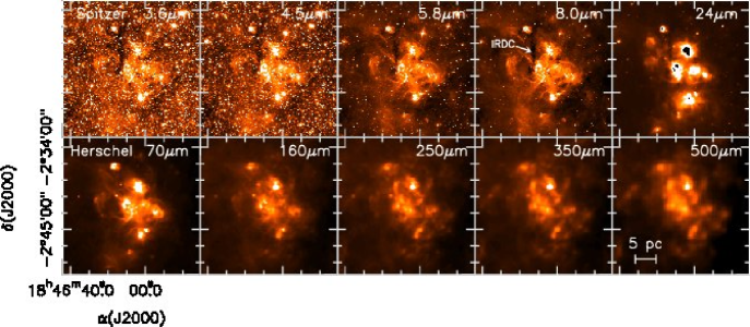
Figure 1: Spitzer 3.6, 4.5, 5.8, 8.0, and 24 $\mu$m and Herschel 70, 160, 250, 350, and 500 $\mu$m images in linear scale of the G29-SFR cloud. The white arrow in the 8.0 $\mu$m image points to the filamentary IRDC (Pillai et al. pillai11 (2011)).

The G29-SFR cloud also contains a filament seen in absorption in the Spitzer images (Fig. 1) and in emission in the SCUBA Massive Pre-/Proto-cluster core Survey (SCAMPS: Thompson et al. thompson05 (2005)) at about $2^{\prime}$ east of the G29-UC region (see Spitzer image at 8 $\mu$m in Fig. 1). This Infrared Dark Cloud (IRDC) has been extensively studied at high-angular resolution in dust continuum emission and NH₂D by Pillai et al. (pillai11 (2011)), who have resolved, with an angular resolution better than $5^{\prime\prime}$, the dust and line emission of the filament into multiple massive cores with low temperatures, $<20$ K, and a high degree of deuteration. These findings support the idea that this massive IRDC is in a very early stage of evolution, and could be in a pre-cluster phase. Only the brightest millimeter continuum core shows signs of high-mass star-formation activity, as indicated by the point source already visible at 24 $\mu$m that is driving a molecular outflow. That no active star formation has been detected in other parts of this IRDC (Pillai et al. pillai11 (2011)) supports the idea of this extincted filament being in a very early evolutionary phase.

As just seen, the G29-SFR cloud represents an ideal laboratory to study star formation because young stellar objects in different evolutionary stages and different masses are embedded in it. In this paper, we present a far-infrared (FIR) study of this cloud using the Hi-GAL data in the 2 PACS and 3 SPIRE photometric bands, centered at 70, 160, 250, 350, and 500 $\mu$m. Our goal is to identify the FIR sources associated with this high-mass star-forming region and estimate their physical properties (mass, temperature, luminosity, and density) together with the Clump Mass Function (CMF) of the cloud. Combining the data with ${\it Spitzer}$ and radio continuum observations, we will investigate the evolutionary stage of the sources and their distribution in the cloud, and the physical parameters of the associated Hii regions. Finally, we will derive the star formation efficiency and star formation rate in this cloud. This work complements the other wide-field studies carried out as part of the Hi-GAL SDP (e.g. Bally et al. bally10 (2010); Battersby et al. battersby11 (2011); Olmi et al. olmi13 (2013)).

2 Source selection

The first step to identify the Hi-GAL sources associated with the G29-SFR cloud is to define the limits of the molecular cloud. To study the distribution of the gas in the region we have used the ¹³CO (1–0) data of the Boston University–Five College Radio Astronomy Observatory Galactic Ring Survey (GRS: Jackson et al. jackson06 (2006)). Towards the direction of the G29-UC region, the ¹³CO (1–0) emission shows relatively narrow components at $\sim$8, 49, and 68 km s^-1, and a much broader component from $\sim$90 to 110 km s^-1. Taking into account that the systemic velocity of high-density tracers, such as NH₃ or CH₃CN, observed towards the G29-HMC core is $\sim$98–99 km s^-1 (Cesaroni et al. cesa98 (1998); Beltrán et al. beltran11 (2011)), we selected the latter broad velocity component to determine the distribution of the gas in the cloud. The ¹³CO (1–0) emission has been averaged over the 95–105 km s^-1 velocity interval and compared with the Hi-GAL 250 $\mu$m emission. As one can see in Fig. 2, the gas and dust emission are very well correlated. The G29-SFR cloud has been defined as the region contained approximately within the contour at 10-15$\%$ of the ¹³CO peak emission (5 K) and that at 7$\%$ of the 250 $\mu$m peak emission (36311 MJy/sr). Only the Hi-GAL sources falling inside this region have been assigned to the G29-SFR cloud.

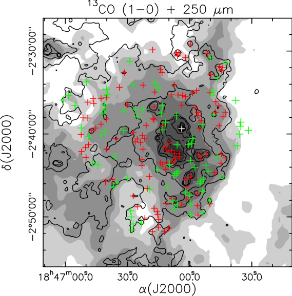
Figure 2: Hi-GAL 250 $\mu$m emission (contours) of the G29-SFR cloud overlaid on the ¹³CO (1–0) emission (grayscale) from GRS averaged over the 95–105 km s^-1 velocity interval. Contour levels are 7, 9, 14, 18, 24, 36, 48, 72, and 96$\%$ of the peak of the 250 $\mu$m emission, 36311 MJy/sr. Grayscale levels are 10, 15, 20, 40, 60, 80, and 100$\%$ of the peak of the ¹³CO emission, 5 K. The crosses indicate the positions of the Hi-GAL sources associated with the cloud detected in the 5 Hi-GAL photometric bands. Red and green crosses indicate, respectively, sources associated and non-associated with Spitzer 24 $\mu$m emission. The white cross marks the position of the Hi-GAL source associated with the G29-UC region and G29-HMC core (see $\S$ 3.2), which is also associated with 24 $\mu$m emission.

2.1 Source extraction

The source extraction and brightness estimation techniques applied to the Hi-GAL maps in this work are similar to the methods used during analysis of the BLAST05 (Chapin et al. chapin08 (2008)) and BLAST06 data (Netterfield et al. netterfield09 (2009); Olmi et al. olmi09 (2009)). However, important modifications have been applied to adapt the technique to the SPIRE/PACS maps. The method used here defines in a consistent manner the region of emission of the same volume of gas/dust at different wavelengths, thus differing from the source grouping and band-merging procedures described by Molinari et al. (molinari11 (2011)) and Elia et al. (elia10 (2010)). Candidate sources are identified by finding peaks after a Mexican Hat Wavelet type convolution is applied to all five SPIRE/PACS maps. Initial candidate lists from 70, 160 and $250\,\mu$m are then found and fluxes at all three bands extracted by fitting a compact Gaussian profile to the source. Sources are not identified at 350 and $500\,\mu$m due to the greater source-source and source-background confusion resulting from the lower resolution, and also because these two SPIRE wavebands are in general more distant from the peak of the source Spectral Energy Distribution (SED). Each temporary source list at 70, 160 and $250\,\mu$m is then purged of overlapping sources and then all three lists are merged. After selecting the sources based on their integrated flux and allowed angular diameter, a final source catalog is generated. In the next stage, Gaussian profiles are fitted again to all SPIRE/PACS maps, including the 350 and $500\,\mu$m wavebands, using the size and location parameters determined at the shorter wavelengths during the previous steps (the size of the Gaussian is convolved to account for the differing beam sizes). Since the volume of emission is basically defined using the 250 $\mu$m band, this method does not fully exploit the higher angular resolution available at the shortest wavelengths. The interested reader can find more details in Olmi et al. (olmi13 (2013)).

The total number of Hi-GAL sources associated with the G29-SFR cloud is 198. The position of the sources in equatorial and galactic coordinates, their fluxes in the 5 photometric Hi-GAL bands, and their possible association with MIPSGAL 24 $\mu$m sources are given in Table 1.

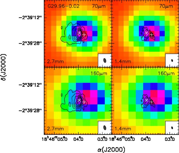
Figure 3: Overlay of the 2.7 mm (left panels) and the 1.4 mm (right panels) continuum emission (contours) obtained with the PdBI (Beltrán et al. beltran11 (2011)) on the Hi-GAL 70 $\mu$m (upper panels) and 160 $\mu$m (lower panels) emission (grayscale) towards the position of the G29-UC region and the G29-HMC core. The white X marks the position of the G29-UC region (Wood & Churchwell wood89 (1989)) and the white cross the position of the 1.4 mm continuum emission peak associated with the G29-HMC core (Beltrán et al. beltran11 (2011)). The contour levels are 3, 9, 18, 27, 39, 51, and 75 times 3 mJy beam^-1 at 2.7 mm and 6.7 mJy beam^-1 at 1.4 mm. The PdBI synthesized beam is shown in the lower righthand corner.

3 Analysis

3.1 Spectral Energy Distribution fitting

To estimate the dust temperature $T$, the mass $M_{\rm env}$, and the luminosity $L_{\rm bol}$, of the sources associated with the G29-SFR cloud, we fitted their observed SED with a modified blackbody of the form $B_{\nu}(T)(1-e^{-\tau_{\nu}})\Omega_{S}$, where $B_{\nu}(T)$ is the Planck function at a frequency $\nu$ for a dust temperature $T$, $\tau_{\nu}$ is the dust optical depth taken as $\tau_{\nu}\propto\nu^{\beta}$, where $\beta$ is the dust emissivity index, and $\Omega_{S}$ is the source solid angle. The source size $\theta$, which is not deconvolved, was estimated at 160 $\mu$m by the source extraction process (Olmi et al. olmi13 (2013)). The masses were calculated assuming a dust mass absorption coefficient of 0.5 cm²/g at 1.3 mm (Kramer et al. kramer03 (2003)) and a gas-to-dust ratio of 100. To check whether the SED fitting improved, we searched for counterparts of the Hi-GAL sources at shorter wavelengths in the MIPSGAL 24 $\mu$m catalog (Shenoy et al. shenoy12 (2012)). The method used to associate Hi-GAL and MIPSGAL sources, which was based on both a positional and a color criteria, is described by Olmi et al. (olmi13 (2013)). For the remaining Hi-GAL sources or those sources saturated at 24 $\mu$m, we searched for a counterpart in the Wide-field Infrared Survey Explorer (WISE) catalog at 22 $\mu$m (Wright et al. wright10 (2010)). To associate a WISE source to a Hi-GAL source, we arbitrarily chose the closest WISE source located at $<12^{\prime\prime}$, the WISE angular resolution at 22 $\mu$m (Wright et al. wright10 (2010)). Finally, for the remaining Hi-GAL sources or those sources saturated at 22 $\mu$m, we searched for a counterpart in the Midcourse Space Experiment (MSX) catalog at 21 $\mu$m (Price et al. price01 (2001)). In this case, we arbitrarily associated the closest MSX source located at $<18\aas@@fstack{\prime\prime}3$, the MSX angular resolution at 21 $\mu$m (Price et al. price01 (2001)). We found 103 MIPSGAL sources not saturated at 24 $\mu$m, 11 WISE sources not saturated at 22 $\mu$m, and 6 MSX sources associated with the Hi-GAL ones. The SED fitting was performed using the 5 Hi-GAL bands for 157 sources. For these 157 sources having a counterpart at shorter wavelengths, including the additional point in the SED did not improve the fitting. For 13 sources, only the 160, 250, 350, and 500 $\mu$m Hi-GAL bands were used. For these sources, the flux at 160 $\mu$m, $S_{160\mu m}$, was $\leq S_{250\mu m}$ and including the $S_{70\mu m}$ in the SED clearly worsen the fit. This indicates that the 70 $\mu$m emission is likely tracing a different source component, more associated with the central stellar object, than that traced by the emission at 160 to 500 $\mu$m, more associated with the extended envelope surrounding the central source. The 5 Hi-GAL bands plus the 21 $\mu$m band of MSX were used in the SED fitting for 4 sources. In these cases, $S_{70\mu m}>S_{160\mu m}$ and including the flux at 21 $\mu$m, which is smaller than that at 70 $\mu$m, clearly improved the fitting. For 6 sources, the 5 Hi-GAL bands plus the 22 $\mu$m band of the WISE were used in the fitting. For these sources, $S_{70\mu m}>S_{160\mu m}$ and $S_{70\mu m}>S_{22\mu m}$, and again, including the flux at a shorter wavelength improved the fitting. Finally, for 18 sources, the 5 Hi-GAL bands plus the 24 $\mu$m MIPSGAL band were used. For these sources, $S_{70\mu m}>S_{160\mu m}$ and $S_{70\mu m}>S_{24\mu m}$, and as in the previous cases, including the flux at a shorter wavelength improved the fitting. The MSX flux at 21 $\mu$m, the WISE flux at 22 $\mu$m, and the MIPSGAL flux at 24 $\mu$m used for the SED fitting of these 28 sources is given in Table 2. Table 3 shows the values of $\theta$, obtained from the source extraction process, of $\beta$, $T$, $M_{\rm env}$, and $L_{\rm bol}$, obtained from the SED fitting, and of the surface density $\Sigma$, for the 198 sources. The surface density was calculated following the expression $\Sigma=M_{\rm env}/(\pi\times R^{2})$, where the radius of the sources $R$ was obtained from their sizes, $\theta$, and following the expression $R=\theta/2\times d$, where $d$ is the distance to the G29-SFR cloud.

Table 4: Mean (median) physical parameters of the Hi-GAL sources

	All sources	24$\mu$m-dark	24$\mu$m-bright
Radius (pc)	0.36 (0.36)	0.34 (0.35)	0.37 (0.38)
Mass ($M_{\odot}$)	379 (115)	435 (172)	340 (86)
Surface density (g cm-2)	0.24 (0.06)	0.27 (0.1)	0.22 (0.04)
Temperature (K)	29 (25)	22 (22)	33 (30)
Luminosity ($L_{\odot}$)	$6.2\times 10^{3}$ (470)	706 (247)	$1\times 10^{4}$ (713)
Luminosity-to-mass ratio ($L_{\odot}/M_{\odot}$)	23 (5)	6 (2)	34 (10)

3.2 The Hi-GAL source associated with the G29-UC region and G29-HMC core

Figure 3 shows an overlay of the continuum emission at 2.7 and 1.4 mm obtained with the IRAM-Plateau de Bure interferometer (PdBI) (Beltrán et al. beltran11 (2011)) on the Hi-GAL maps at 70 and 160 $\mu$m towards the position of the G29-UC region and G29-HMC core. The Hi-GAL source in our catalog is #242. As seen in Table 1, this is the brightest source in all 5 Hi-GAL bands. At 2.7 and 1.4 mm, the G29-UC region is outlined by continuum emission showing a cometary arc shape, while the G29-HMC core emission is visible westwards in front of the arc. The emission of the G29-HMC core is better resolved at 1.4 mm, where it shows a flattened structure. The peak of the 1.4 mm continuum emission (Beltrán et al. beltran11 (2011)), indicated with a white cross in Fig. 3, coincides with the G29-HMC core. As one can see in this figure, at 70 $\mu$m, the emission seems to be mainly associated with the G29-HMC core. In fact, the peak of the 70 $\mu$m emission coincides with that of the 1.4 mm continuum emission. At 160 $\mu$m, the emission also seems to be more associated with the HMC than with the UC Hii region, although in this case the peak of the Hi-GAL emission is located towards the north of the G29-HMC core. The angular resolution of the Hi-GAL emission at 250, 350, and 500 $\mu$m is not enough to properly study with which component, the HMC or the UC Hii region, this sub-millimeter emission is associated.

Figure 4: SED of the Hi-GAL source #242, associated with the G29-UC region and G29-HMC core. The black circles and black square show the Hi-GAL and MSX at 21 $\mu$m data, respectively, with error bars. The black solid line represents the best-fit modified blackbody.

Figure 5: Histograms of some parameters of the Hi-GAL sources detected towards G29: a) radius of the sources; b) mass; c) H₂ surface density; d) temperature; e) luminosity; and f) luminosity-to-mass ratio. The dotted line in panel $c$ indicates the minimum surface density needed to form massive stars according to theory (Butler & Tan butler12 (2012)).

From the SED fitting (Fig. 4), we derived a mass of $\sim$2880 $M_{\odot}$ for source #242, for a dust temperature of 77 K, the highest of the sources in the G29-SFR cloud, a size of $\sim$$19^{\prime\prime}$, and a dust emissivity index of 0.8. The surface density is 2.3 g cm^-2, well above the theoretical threshold of 1 g cm^-2 (Krumholz & McKee krumholz08 (2008)) necessary for high-mass star formation to occur. The luminosity of this source is $\sim$$8\times 10^{5}$ $L_{\odot}$ and is the highest in the whole cloud. Kirk et al. (kirk10 (2010)) constructed the SED of this source by using the SPIRE Fourier Transform Spectrometer data from 190 to 670 $\mu$m and archival data from 2.4 to 1.3 mm (see their Fig. 1). From the SED fitting, these authors obtained a temperature of $\sim$80 K, in agreement with our value, and a dust emissivity index of $\sim$1.7, twice the one that we obtained. The dust luminosity integrated under the fitted modified blackbody in the range 2–2000 $\mu$m is $1.6\times 10^{6}$ $L_{\odot}$, assuming a distance of 8.9 kpc. The luminosity would be $\sim$$8\times 10^{5}$ $L_{\odot}$ for a distance of 6.2 kpc, in agreement with our estimated $L_{\rm bol}$. As for the mass, Kirk et al. (kirk10 (2010)) estimate a mass of 1500 $M_{\odot}$, assuming a distance of 8.9 kpc, using the fitted dust temperature and the SCUBA 850 $\mu$m flux density (Thompson et al. thompson06 (2006)). The mass would be $\sim$730 $M_{\odot}$ for a distance of 6.2 kpc. This value is a factor $\sim$4 smaller than the one that we obtained from the SED fitting. Besides the different method used to estimate the mass, this difference could be accounted for, in part, by the different opacity coefficient (0.01 cm²/g at 850 $\mu$m) and dust emissivity index ($\beta$=1.7) used by these authors.

3.3 Source physical parameters

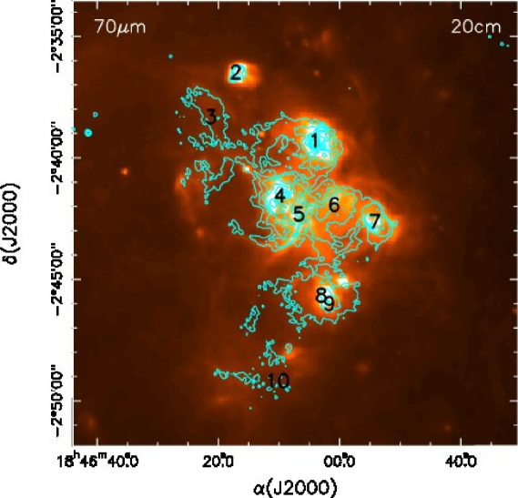
Figure 6: 20 cm continuum emission from the MAGPIS survey (cyan contours) of the G29-SFR cloud overlaid on the Hi-GAL 70 $\mu$m emission (colors). Contour levels are 3, 6, 12, 24, 48, 96, and 192 times 1 mJy beam^-1. The numbers indicate the positions of the 10 NVSS sources. The synthesized beam of the 20 cm MAGPIS observations is $6\aas@@fstack{\prime\prime}2\times 5\aas@@fstack{\prime\prime}4$ at P.A. = 0$\degr$

Figure 5 shows the distribution of radii, masses, surface densities, temperatures, luminosities and luminosity-to-mass ratios of the sources. Table 4 shows the mean and median values for the same physical quantities. Beltrán et al. (beltran06 (2006)) observed a sample of southern hemisphere high-mass protostellar candidates at 1.2 mm with the SEST antenna. In the following we will confront the physical parameters obtained for the sources in the G29-SFR cloud with those of Beltrán et al. (beltran06 (2006)) because them carried out a detailed comparison of the values of their sources with those estimated in other millimeter continuum surveys. The mean and median values of 0.36 pc for the radius of the Hi-GAL sources associated with the G29-SFR cloud suggest that these sources are probably clumps (e.g. Giannini et al. giannini12 (2012)) that will not form individual stars but multiple star systems or star clusters. Unfortunately, the Herschel observations do not have enough spatial resolution to resolve these clumps into individual cores or stars. These values of the radius are consistent with the mean and median values of 0.25 and 0.2 pc found by Beltrán et al. (beltran06 (2006)). The mean and median values of the mass are also consistent with the mean and median values of 320 and 102 $M_{\odot}$ found by Beltrán et al. (beltran06 (2006)) for their sample, and indicates that the sources associated with the G29-SFR cloud and detected by ${\it Herschel}$ are mostly massive objects. The mean temperature is in agreement with the mean temperature of 28 K found by Beltrán et al. (beltran06 (2006)), and with the value of 32 K found by Molinari et al. (molinari00 (2000)) for a sample of luminous high-mass protostellar candidates in the northern hemisphere.

The average and median values of the surface density, of 0.24 and 0.06 g cm^-2, are similar to the mean and median values of 0.4 and 0.14 g cm^-2 estimated by Beltrán et al. (beltran06 (2006)). These values are slightly lower than the minimum surface density needed, according to theory (Krumholz & McKee krumholz08 (2008)), to form massive stars. In a recent work, Butler & Tan (butler12 (2012)) find typical mass surface densities of 0.15 g cm^-2 for cores, and of 0.3 g cm^-2 for clumps in infrared dark clouds, some of which are likely to form massive stars. Butler & Tan (butler12 (2012)) consider the cores as structures of about 100 $M_{\odot}$ embedded in clumps. These cores, which are virialized and in approximate pressure equilibrium with the surrounding clump environment, are undergoing global collapse to feed a central accretion disk. On the other hand, the clump is defined as the gas cloud that fragments to form a star cluster. These authors propose that fragmentation in these clumps could be inhibited by magnetic fields rather than radiative heating and that the initial conditions of local massive star formation in the Galaxy may be better characterized by surface density values of $\sim$0.2 g cm^-2 rather than 1 g cm^-2. This would imply smaller accretion rates and longer formation timescales ($>10^{5}$ yr) for massive stars than those predicted my McKee & Tan (mckee03 (2003)).

The mean luminosity estimated, $6.2\times 10^{3}$ $L_{\odot}$, would correspond to a main-sequence star of spectral type B1 following Table 1 of Mottram et al. (mottram11 (2011)), and thus, it also indicates that the Hi-GAL sources associated with the G29-SFR cloud are mostly high-mass sources. Note, however, that this value is an order of magnitude smaller than the average value of $6.7\times 10^{4}$ $L_{\odot}$ obtained by Beltrán et al. (beltran06 (2006)) for a sample of massive protostellar candidates. This is not surprising, taking into account that the bolometric luminosities calculated by these authors are to be considered upper limits because estimated from the IRAS flux densities. The IRAS beam is so large ($\sim$2^′) that when integrating the flux density for a single protostellar candidate, there might be an important contribution not only from other sources that may fall into such a large beam, but also from inter-clump diffuse emission. The latter contribution is subtracted out when doing the source extraction but is included if one simulates what would be seen with a larger beam like that of IRAS.

The luminosity-to-mass ratio, $L_{\rm bol}/M_{\rm env}$, is an important parameter for establishing the age of a source. This ratio is expected to increase with time as more gas is incorporated into the star that becomes more luminous. The mean and median $L_{\rm bol}/M_{\rm env}$ values for the sources in the G29-SFR cloud are 23 and 5 $L_{\odot}/M_{\odot}$, respectively, which are significantly lower than the average and median values of 99 $L_{\odot}/M_{\odot}$ obtained by Beltrán et al. (beltran06 (2006)). However, as already mentioned, this discrepancy could be due to the fact that the bolometric luminosities of the sources in the Beltrán et al. sample are likely upper limits because they were estimated from the IRAS fluxes.

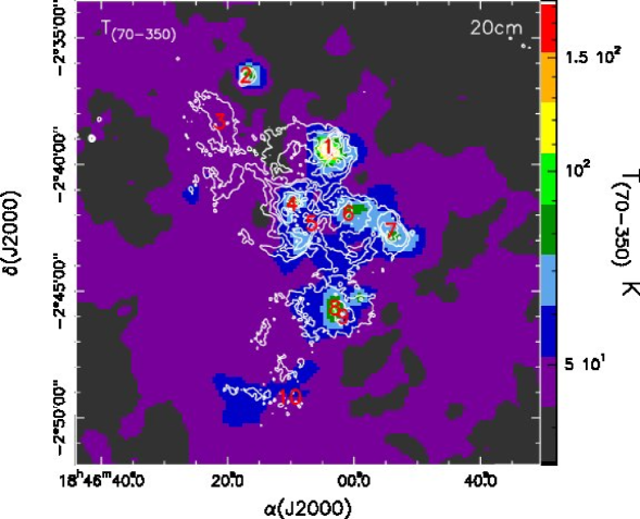
Figure 7: 20 cm continuum emission from the MAGPIS survey (blue contours) of the G29-SFR cloud overlaid on the 70–350 $\mu$m color temperature map in logarithmic scale (colors). Contour levels and numbers are the same of Fig. 6.

3.4 Centimeter emission associated with the G29-SFR cloud

Figure 6 shows a zoom-in towards the central region of the G29-SFR cloud. In this figure, the 20 cm emission of the Multi-Array Galactic Plane Imaging Survey (MAGPIS: Helfand et al. helfand06 (2006)) is overlaid on the Hi-GAL 70 $\mu$m emission. The angular resolution of both sets of data is similar, which makes the comparison straightforward. The positions of the ten 21-cm sources associated with the cloud from the NRAO/VLA Sky Survey (NVSS: Condon et al. condon98 (1998)) catalog at 1.4 GHz are also indicated in the figure. NVSS source #1 is associated with the G29-UC region and with Hi-GAL source #242. Table 5 gives the coordinates, flux densities at 21 cm, and major and minor axes of the NVSS sources after deconvolving with the restoring beam of 45^′′ of the NVSS images. The source fluxes have been obtained from the NVSS catalog instead of estimating them directly from the MAGPIS map at 20 cm because of the better surface brightness sensitivity of NVSS. The deconvolved sizes for five out of ten sources are upper limits, which indicates that either the source is unresolved or that the emission is too large to properly fit it with just one Gaussian (Condon et al. condon98 (1998)). The latter is the case for NVSS source #10, which, as seen in Fig. 6, is very extended and with a very low-level emission, and therefore difficult to fit with a Gaussian. Figure 7 shows the 20 cm continuum emission overlaid on the 70–350 $\mu$m color temperature, $T_{(70-350)}$, map. To calculate the color-color temperature map, we first smoothed the 70 $\mu$m map (that with the highest angular resolution: $9\aas@@fstack{\prime\prime}2$) to the resolution of the 350 $\mu$m map ($25^{\prime\prime}$), and then reprojected both maps to the same pixel and map size. These two wavelengths happen to bracket the peak of the SED and are hence most sensitive to temperature changes. Clearly, the colour temperature is a proxy for the dust temperature, but may differ significantly from the temperature estimate obtained by fitting the whole SED with a modified blackbody. As seen in Fig. 7, the positions of the NVSS sources, except for the very diffuse NVSS sources #3 and 10, coincide with local maxima of the color-color temperature.

Table 5: Position, fluxes, and sizes of the NVSS sources associated with the G29-SFR cloud

	$\alpha({\rm J2000})$	$\delta({\rm J2000})$	$S_{21\,{\rm cm}}$	Major axis	Minor axis
# Id.	(h m s)	($\degr$ $\arcmin$ $\arcsec$)	(Jy)	(′′)	(′′)
1a	18 46 04.09	$-$2 39 19.1	2.38	26.6	20.4
2	18 46 17.11	$-$2 36 30.0	0.025	$<$26.3	$<$18.4
3	18 46 21.24	$-$2 38 20.3	0.035	63.5	31.2
4	18 46 09.83	$-$2 41 34.9	3.06	49.3	44.7
5	18 46 06.69	$-$2 42 20.8	1.55	127.3	50.1
6	18 46 00.89	$-$2 41 57.4	0.137	$<$14.2	$<$14.1
7	18 45 54.17	$-$2 42 39.0	0.435	35.6	24.5
8	18 46 03.00	$-$2 45 41.0	0.097	$<$80.3	$<$21.6
9	18 46 01.67	$-$2 46 01.6	0.052	$<$15.5	$<$15.3
10	18 46 10.25	$-$2 49 12.3	0.010	$<$125.9	$<$125.0

^a G29-UC and Hi-GAL source #242.

Table 6: Physical parameters of the Hii regions in the G29-SFR cloud

	$R$	$T_{B}$	$n_{e}$	$EM$	$N_{\rm Ly}$	$M_{\rm ion}$	Spectral
# Id.	(pc)	(K)	(cm-3)	($10^{5}$ cm-6 pc)	($10^{47}$ s-1)	($M_{\odot}$)	Type
1a	0.35	274	2028	19	84	9.0	O6
2	$<$0.33	$>$32	$>$226	$>$0.23	0.88	$<$0.85	B0
3	0.67	11	93	0.08	1.2	2.9	B0
4	0.71	865	803	6	108	29	O5
5	1.2	152	258	1	55	46	O6.5
6	$<$0.21	$>$426	$>$1027	$>$3	4.8	$<$1.0	O9.5
7	0.44	311	607	2	15	5.5	O8.5
8	$<$0.63	$>$35	$>$171	$>$0.24	3.4	$<$4.3	09.5
9	$<$0.23	$>$136	$>$557	$>$0.96	1.8	$<$0.71	B0
10	$<$1.9	$>$0.4	$>$ 10	$>$0.003	0.35	$<$7.2	B0.5

^a G29-UC and Hi-GAL source #242.

As seen in Fig. 6, the centimeter emission is well correlated with the 70 $\mu$m emission, even at the low level emission. Note how both the centimeter and the FIR emission trace the arcs seen eastwards of NVSS sources #4 and 5. These arcs are shock fronts where hydrogen is ionized, and gives rise to the radio continuum. It is also possible that important shock gas coolants like the [OI 63 $\mu$m] line could be in part contaminating the PACS 70 $\mu$m emission. The fact that the centimeter emission is so extended and well correlated with the dust emission would suggest that it is associated with a group of Hii regions that are ionizing and disrupting the cloud. Assuming that the centimeter continuum emission comes from homogeneous optically thin Hii regions, we calculated the physical parameters of the 10 NVSS sources (using the formalism of Mezger & Henderson mezger67 (1967) and Rubin rubin68 (1968)) and list them in Table 6. Column 1 gives the NVSS number of the source (Table 5), column 2 the spatial radius $R$ of the Hii region, which was determined from the deconvolved source size (Table 5), column 3 the source averaged brightness $T_{B}$, column 4 the electron density $n_{e}$, column 5 the emission measure $EM$, column 6 the number of Lyman-continuum photons per second $N_{\rm Ly}$, column 7 the mass of ionized gas $M_{\rm ion}$, which was calculated assuming a spherical homogeneous distribution, and column 8 the spectral type of the ionizing source. The spectral type was computed from the estimated $N_{\rm Ly}$ and using the tables of Davies et al. (davies11 (2011)) and Mottram et al. (mottram11 (2011)), which are for Zero Age Main Sequence (ZAMS) stars. Note that if the 21 cm emission is optically thick, then $T_{B}$, $n_{e}$, $EM$, $N_{\rm Ly}$, $M_{\rm ion}$, and therefore, the spectral type should be considered as lower limits. For the sources with upper limits for the deconvolved sizes (Table 5), $R$ and $M_{\rm ion}$ should be taken as upper limits, while $T_{B}$, $n_{e}$ and $EM$ as lower limits. As seen in Table 6, most of the sources are early B or late O types. However, the cloud would also contain 3 sources, with one of them being the G29-UC region (NVSS source #1), with spectral types O5–O6.5. Therefore, it is possible that these massive sources, with their strong winds and radiation pressure, are disrupting and shaping the cloud. This effect may contribute to underestimate the number of ionizing photons and, in turn, the luminosities of the stars. Note that sources #4 and 5, located at the head of the large arc-like structure seen towards the east, have spectral types O5 and O6.5, respectively.

3.5 Physical parameters as a function of the distance to the NVSS sources in the G29-SFR cloud

To check whether there is a variation of the Hi-GAL source physical parameters as a function of the distance to the most massive sources in the G29-SFR cloud, we plotted the distribution of masses, surface densities, luminosities, temperatures, and luminosity-to-mass ratios of the Hi-GAL sources as a function of the distance to the NVSS sources #1, 4, 5, 6, and 8 (Fig. 8). The NVSS sources #2, 3, 7, and 10 have not been taken into account because are located close to the border of the cloud. NVSS source #9 is located very close to NVSS source #8, and therefore, the distributions should be very similar. The data have been binned in intervals of $\sim$80^′′. For NVSS source #1 (G29-UC), only one Hi-GAL source (#242) is found in the first interval of $\sim$80^′′, which means that the first point in the plots takes into account only the physical parameters of this source.

The physical parameters of NVSS source #1 (G29-UC) and its immediate surroundings have the highest values of all the centimeter sources in the G29-SFR cloud. This is evident in Fig. 8 when comparing NVSS source #1 to sources #4, 5, 6, and 8, but it is also true for the rest of NVSS sources not shown in this plot. Given the large error bars in Fig. 8, one can only see a marginal trend of the mass and surface density, which seem to decrease with the distance from NVSS source #1. The surface density is above the minimum value of 0.2 g cm^-2 needed to form massive stars according to theory (Butler & Tan butler12 (2012)), up to a distance of $\sim$150^′′ from the G29-UC region. A similar marginal trend is seen for NVSS source #4. Although in this case, the decrease in $M_{\rm env}$ is even less obvious, and the surface density is slightly above 0.2 g cm^-2 only in a small region ($\lesssim 80^{\prime\prime}$) surrounding the source. Regarding the luminosity, temperature and luminosity-to-mass ratio, again, the highest values are found towards the NVSS source #1 (G29-UC).

Figure 8: Distributions of mass, surface density, temperature, luminosity, and luminosity-to-mass ratio as a function of the distance to the NVSS sources in the G29-SFR cloud. The NVSS number (Tables 5 and 6) is indicated in the lefthand upper corner of the upper panels. The dotted line in the surface density distributions indicates the minimum value needed needed to form massive stars according to theory (Butler & Tan butler12 (2012)). The first bin contains only one point and, thus, the standard deviation is zero.

The fact that the most massive and luminous Hi-GAL sources in the cloud are located close to the strongest source in the G29-SFR cloud (#242 or G29-UC) suggest that there is a privileged area for massive star formation in the cloud. Based on the central location of the G29-UC region inside the G29-SFR cloud (Fig. 2), this indicates that high-mass stars form preferentially at the center of the cloud, as expected. An inhomogeneous density distribution of the cloud, with higher density towards the center of the cloud (maybe already present as an initial condition), could be responsible for this source distribution. This is consistent with the findings of most millimeter continuum surveys.

3.6 24$\mu$m-dark versus 24$\mu$m-bright sources

Because star formation does not occur simultaneously all over a cloud, one would expect to find young stellar objects in different evolutionary stages associated with the G29-SFR cloud. To search for differences in the evolutionary stage of the sources, we cross-correlated our Hi-GAL sources with the Spitzer MIPSGAL 24 $\mu$m catalog. The last column in Table 1 indicates whether a source is associated or not with 24 $\mu$m emission. Obviously, we counted as associated those sources saturated at 24 $\mu$m, like for example the Hi-GAL source #242 (G29-UC). Based on this association, we divided the sources into two groups: those without a 24 $\mu$m counterpart, that we call 24$\mu$m-dark, and those with a 24 $\mu$m counterpart, that we call 24$\mu$m-bright. The former are expected to be the youngest Hi-GAL sources in the cloud. As a result of this cross-correlation we discovered 81 Hi-GAL sources not associated with 24 $\mu$m emission and 117 Hi-GAL sources associated with it. As shown in Fig. 2, both kind of Young Stellar Objects (YSOs) are uniformly distributed over the cloud.

Figure 9: Histogram of the [70–160] color for 24 $\mu$m-bright (solid line) and 24 $\mu$m-dark (dashed line) sources.

All the sources in our sample have been selected to be detected in all 5 photometric Hi-GAL bands. Therefore, by definition, all the sources have been detected at 70 $\mu$m, which would suggest that most of them, if not all, are protostellar. However, this does not mean that there are no prestellar sources in the G29-SFR cloud (see Pillai et al. pillai11 (2011)). The analysis of the sources not detected at 70 $\mu$m, and likely prestellar, although being highly interesting, goes beyond the scope of the present study. To check whether 24$\mu$m-dark and 24$\mu$m-bright sources show any difference in their 70 $\mu$m fluxes, we plotted and histogram of the [70–160] color for both kind of sources (Fig. 9). As seen in this figure, the [70–160] color of 24$\mu$m-dark sources is clearly smaller than those of the 24$\mu$m-bright ones. This indicates that the possible different evolutionary phase of the sources is also supported by the Hi-GAL data.

Figure 10 shows the distribution of radii, masses, surface densities, temperatures, luminosities and luminosity-to-mass ratios for 24$\mu$m-dark and 24$\mu$m-bright sources. Table 4 shows the mean and median values for the same physical quantities. One sees that the distributions of the two types of objects are different. A closer inspection of the data using the Kolmogorov-Smirnov (KS) statistical test shows that, except for the radius distributions, the probability of the mass, surface density, temperature, luminosity, and luminosity-to-mass ratio distributions being the same for 24$\mu$m-dark and 24$\mu$m-bright sources is very low ($P$ $\lesssim$ 0.004). Therefore, the physical properties of the two groups are statistically different. The temperature, luminosity, and, in particular, the luminosity-to-mass ratio are smaller for the 24$\mu$m-dark than for the 24$\mu$m-bright objects, while the mass and the surface density are higher. That $T_{d}$, $L_{\rm bol}$, and $L_{\rm bol}/M_{\rm env}$ are smaller for 24$\mu$m-dark than for 24$\mu$m-bright sources is consistent with the former being in an earlier evolutionary phase. Figure 10 also shows that a relatively large number of 24$\mu$m-dark and 24$\mu$m-bright sources have surface densities high enough to form massive stars according to theory (Butler & Tan butler12 (2012)).

Figure 10: Histograms of a) radius of the sources; b) mass; c) H₂ surface density; d) temperature; e) luminosity; and f) luminosity-to-mass ratio, for 24 $\mu$m-bright (solid line) and 24 $\mu$m-dark (dashed line) sources. The dotted line in panel $c$ indicates the minimum surface density needed to form massive stars according to theory (Butler & Tan butler12 (2012)).

The most significant difference between the two groups is found in the value of $L_{\rm bol}/M_{\rm env}$. In fact, the mean and median value of $L_{\rm bol}/M_{\rm env}$ is $\sim$6 and $\sim$5 times lower for the 24 $\mu$m-dark sources compared to the 24 $\mu$m-bright ones, which supports our assumption that the sources not associated with 24 $\mu$m emission are in an earlier evolutionary phase.

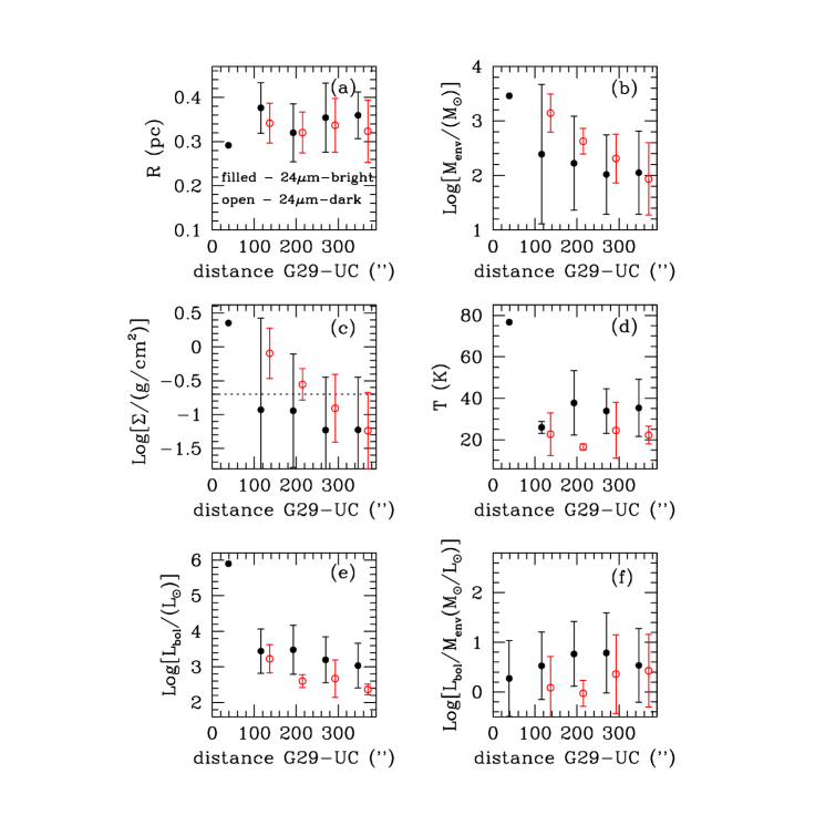
Figure 11: Distributions of a) radius of the sources; b) mass; c) H₂ surface density; d) temperature; e) luminosity; and f) luminosity-to-mass ratio as a function of the distance to the G29-UC region for 24 $\mu$m-bright (filled circles) and 24 $\mu$m-dark (open red circles) sources. The dotted line in the surface density distributions indicates the minimum value needed to form massive stars according to theory (Butler & Tan butler12 (2012)). The first bin contains only one point and, thus, the standard deviation is zero.

We also investigated whether the radii, masses, surface densities, temperatures, luminosities and luminosity-to-mass ratios of the two types of sources show any correlation as a function of the distance to the G29-UC region. Figure 11 indicates that both groups show the same trends, that is, the mass, surface density, and luminosity of the sources marginally decrease when moving away from the G29-UC region, while the size, temperature and luminosity-to-mass ratio, except for the high values close to the G29-UC region, do no significantly change.

4 Discussion

4.1 Evolutionary phase of the sources

To investigate the stability of the sources, we calculated their Jeans masses, $M_{J}$, and virial masses, $M_{\rm virial}$. $M_{J}$ was calculated following the expression $M_{J}=[T/10\,{\rm K}]^{3/2}\times[n_{\rm H_{2}}/1\times 10^{4}\,{\rm cm^{-3}}]^{-1/2}$, where the dust temperature $T$ was obtained from the SED fitting and the H₂ volume density $n_{\rm H_{2}}$ was calculated assuming that the sources have spherical symmetry (the size of the sources is that obtained from the source extraction process). $M_{\rm virial}$ was estimated from the line width, $\Delta V$, of ¹³CO (1–0) towards the position of each source following the expression of MacLaren et al. (macLaren88 (1988)), $M_{\rm virial}=0.509\times d\times\theta\times\Delta V^{2}$, where $d$ is the distance in kpc, $\theta$ is the size of the source in arcsec obtained from the source extraction process, and $\Delta V$ is in km s^-1. The choice of ¹³CO (1–0) to estimate the virial masses, which could be partially optically thick and therefore overestimate the line width, is based on the fact that it is the only molecular tracer covering the whole cloud. To have an idea of how large the overestimate of the line widths could be, we checked the value towards source #242 (associated with the G29-UC region and G29-HMC core), which has been extensively observed in different molecular tracers. The line width estimated with ¹³CO is 6.2 km s^-1 and is similar to the values of $\sim$5.5 km s^-1 estimated in CS (5–4) and (7–6), and HCO⁺ (3–2) with the JCMT and the IRAM 30-m telescopes (Olmi et al. olmi99 (1999); Churchwell et al. churchwell10 (2010)). $M_{\rm virial}$ depends on the density profile, and for a power-law density distribution of the type $\rho\propto r^{-p}$, the virial mass should be multiplied by a factor $3(5-2p)/5(3-p)$, which is $\leq 1$ for $p<3$. Thus, the values estimated should be taken as upper limits.

Figure 12: Histogram of a) the mass-to-Jeans mass ratio and b) mass-to-virial mass ratio for 24 $\mu$m-bright (solid line) and 24 $\mu$m-dark (dashed line) sources. The dotted vertical line indicates a) $M_{\rm env}=M_{J}$ and b) $M_{\rm env}=M_{\rm virial}$.

Figure 12 shows the $M_{\rm env}$–$M_{J}$ ratio and the $M_{\rm env}$–$M_{\rm virial}$ ratio for all the sources, 24 $\mu$m-bright and 24 $\mu$m-dark. As seen in this plot, almost all the sources have masses well above $M_{J}$. In particular, 90% of the 24 $\mu$m-bright sources and 96% of the 24 $\mu$m-dark ones have masses well above $M_{J}$. In fact, the mean and median values of the $M_{\rm env}$–$M_{J}$ ratio are 296 and 14 for 24 $\mu$m-bright sources, and 735 and 86 for 24 $\mu$m-dark sources. This indicates that most of the sources in the G29-SFR cloud would be gravitationally supercritical if only supported by thermal pressure, in which case, they should be collapsing. The $M_{\rm env}$–$M_{\rm virial}$ ratio confirms that an additional supporting agent, such as turbulence, is likely acting against gravity in these sources, because only 5% (6 out of 117 sources) of the 24 $\mu$m-bright sources and 7% (6 out of 81 sources) of the 24 $\mu$m-dark ones have masses above the virial mass. The mean and median values of the $M_{\rm env}$–$M_{\rm virial}$ ratio are 0.2 and 0.07 for 24 $\mu$m-bright sources, and 0.3 and 0.1 for 24 $\mu$m-dark sources.

This result seems to be in contrast with the results of other studies of high-mass star-forming clumps, where the mass of the clumps is found to be larger than the virial mass (e.g. Hofner et al. hofner00 (2000); Fontani et al. fontani02 (2002)). López-Sepulcre et al. (lopez10 (2010)) findings for a sample of 29 IR-bright and 19 IR-dark high-mass cluster-forming clumps are similar to ours, although on average their objects are closer to virial equilibrium. What are the sources of uncertainty in our estimate of the $M_{\rm env}$–$M_{\rm virial}$ ratio? The major problem is that very likely the ¹³CO emission is not tracing the same volume of gas as the 1.2 mm continuum emission. This means that the ¹³CO line width may not be representative of the gas contributing to $M_{\rm env}$. However, to allow for a mean value of $M_{\rm env}/M_{\rm virial}$$=1$, one should shift the distributions in Fig. 12b by an order of magnitude, which implies a decrease of the line width by a factor $\sim$3. This seems too much, as observations of different tracers with different resolutions in high-mass star forming regions reveal changes by only a few km/s, for line widths of several km/s. Another source of error could be the temperature estimate, which enters almost linearly into the calculation of $M_{\rm env}$. It is thus difficult to believe that this effect may contribute by more than 20–30%, by far less than the factor 10 required to match $M_{\rm env}$ to $M_{\rm virial}$. Finally, density gradients may affect the estimate of $M_{\rm virial}$. Assuming a power-law density profile as steep as $\rho\propto R^{-2}$, with $R$ radius of the clump, our values of $M_{\rm virial}$ should decrease only by a factor 0.6 (see MacLaren et al. 1988), still not sufficient to justify the observed ratio $M_{\rm env}$–$M_{\rm virial}$.

We conclude that none of the previous effects can explain the distributions in Fig. 12b. However, it is possible that all of them contribute to the result. While this is certainly possible for a limited number of sources (especially those with $M_{\rm env}/M_{\rm virial}\lesssim 1$), it seems likely that $M_{\rm env}/M_{\rm virial}$ is indeed $<$1 for the majority of the objects.

Assuming that this is the case, it is interesting to note that of the 36 sources located at $\lesssim 4^{\prime}$ of the G29-UC region, 14% (5 sources including source #242: G29-UC) have $M_{\rm env}>M_{\rm virial}$. On the other hand, of the remaining 162 sources, which are located at $>4^{\prime}$, only 4% (7 sources), have $M_{\rm env}>M_{\rm virial}$. Despite the poor statistics, this result seems to suggest that the sources that should be undergoing collapse and forming stars are preferentially concentrated towards the dominant source in the G29-UC cloud.

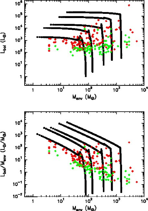
Figure 13: $L_{\rm bol}$–$M_{\rm env}$ (upper panel) and $L_{\rm bol}$/$M_{\rm env}$–$M_{\rm env}$ (lower panel) plots for 24 $\mu$m-bright (red diamonds) and 24 $\mu$m-dark (green diamonds) sources in the G29-SFR cloud. Black lines represent the evolutionary tracks of Molinari et al. (molinari08 (2008)) (see § 4.1). The different models are for different initial masses of 80, 140, 350, 700 and 1500 $M_{\odot}$ (from left to right).

The fact that the sources associated with the G29-SFR cloud appear to be in different evolutionary stages is also suggested by the association or not with Spitzer 24 $\mu$m emission, as already discussed in § 3.6.

To check the validity of this evolutionary phase difference for the sources in the G29-SFR cloud, we decided to use the evolutionary sequence tool of Molinari et al. (molinari08 (2008)). These authors have developed an empirical model to describe the pre-main sequence evolution of YSOs in the high-mass regime based on an $L_{\rm bol}$–$M_{\rm env}$ diagram, where $L_{\rm bol}$ is the bolometric luminosity of the sources, and $M_{\rm env}$ the total envelope mass. Based on the model of collapse in turbulence supported cores of McKee & Tan (mckee03 (2003)), which describes the free-fall accretion of material onto a central source as a time-dependent process, Molinari et al. (molinari08 (2008)) have constructed evolutionary tracks in the $L_{\rm bol}$–$M_{\rm env}$ diagram. According to this evolutionary sequence, sources in different phases should occupy different regions of the $L_{\rm bol}$–$M_{\rm env}$ diagram. For the high-mass regime, the bolometric luminosity of a YSO evolving towards the ZAMS increases by several orders of magnitude during the accretion phase. Therefore, one would expect 24 $\mu$m-dark sources to have a lower $L_{\rm bol}$ than the 24 $\mu$m-bright ones for similar $M_{\rm env}$. Elia et al. (elia10 (2010)) prefer to use the $L_{\rm bol}/M_{\rm env}$ ratio versus $M_{\rm env}$ as a diagnostic, based on the fact that an earlier evolutionary stage source should have smaller $L_{\rm bol}/M_{\rm env}$ ratio than more evolved ones.

As seen in Fig. 13, 24 $\mu$m-dark and 24 $\mu$m-bright sources occupy different regions of the $L_{\rm bol}$–$M_{\rm env}$ and $L_{\rm bol}$/$M_{\rm env}$–$M_{\rm env}$ diagrams, with 24 $\mu$m-dark sources having lower $L_{\rm bol}$ and $L_{\rm bol}$/$M_{\rm env}$ for similar $M_{\rm env}$, as expected. This confirms that the sources not associated with 24 $\mu$m emission are indeed in an earlier evolutionary phase than those associated. In fact, almost all the 24 $\mu$m-dark sources occupy a lower part of the accretion phase of the Molinari et al. evolutionary tracks, while the 24 $\mu$m-bright ones are located closer to the ZAMS, as indicated by the end of the ascending tracks.

4.2 Embedded population in the G29-SFR cloud

As discussed in the previous section, most of the sources in the G29-SFR cloud seem to be in the main accretion pre-main sequence phase or early ZAMS phase (Fig. 13). This seems to indicate that the population in the G29-SFR cloud, mostly massive sources, should be highly embedded. In a recent work, Faimali et al. (faimali12 (2012)) analyze Hi-GAL data on another massive star-forming region G305 and propose a far-IR color criterion to select massive embedded sources. According to these authors, the [70–500] and the [160–350] colors should be most sensitive to the embedded population. Based on the fact that the embedded massive protostars in G305, associated with typical signposts of massive star formation such as free-free emission, water and/or methanol masers, and 24 $\mu$m emission, are confined to an area of $L_{\rm bol}$-color plots, these authors propose that embedded massive star-forming sources, both prestellar and protostellar, should have [70–500] $\geq 1$ and [160–350] $\geq 1.6$ for $L_{\rm bol}>10^{3}\,L_{\odot}$. To check whether these selection criteria for embedded massive sources are valid for our sources, we plot the luminosity versus color in Fig. 14. The distribution of sources is very similar to that found by Faimali et al. (faimali12 (2012)) for the sources in G305. In the G29-SFR cloud, we found 46 24 $\mu$m-bright and 7 24 $\mu$m-dark sources that satisfy the criterion for embedded massive star candidates, a number similar to that found by Faimali et al. (faimali12 (2012)) in G305. This would indicate that only $\sim$27% of the population in the G29-SFR cloud would be embedded massive star candidates. However, as previously mentioned, most of the sources in the G29-SFR cloud seem to be pre-main sequence sources in the main accretion phase or early ZAMS phase, and therefore, embedded. One possible explanation for this discrepancy could be that most of these sources in the G29-SFR cloud have $L_{\rm bol}<$10${}^{3}\,L_{\odot}$, and therefore lie by definition outside the selection criterion area. However, by doing this, the selection criterion would miss those young massive embedded protostars in a very early evolutionary phase that have not yet reached their final luminosity (see Fig. 13).

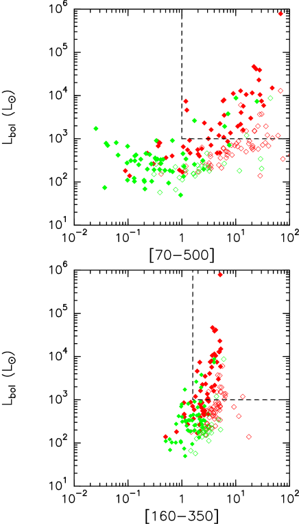
Figure 14: Luminosity–color plots for the Hi-GAL 24 $\mu$m-bright (red diamonds) and 24 $\mu$m-dark (green diamonds) sources in the G29-SFR cloud. The empty red and green diamonds indicate sources with $M_{\rm env}<100\,M_{\odot}$. Dashed lines indicate the threshold of the area defined by Faimali et al. (faimali12 (2012)) for selecting embedded massive YSOs, at a luminosity $>10^{3}\,L_{\odot}$.

The second problem with the Faimali et al. (faimali12 (2012)) selection criterion is that, as shown in Fig. 14, there are a few sources that are clearly not massive ($M_{\rm env}<100\,M_{\odot}$) and have $L_{\rm bol}>$10${}^{3}\,L_{\odot}$ (see Fig. 14) that would fall inside the massive embedded population area. If we lower the limit to $M_{\rm env}<50\,M_{\odot}$, there are still 8 24 $\mu$m-bright sources that would satisfy the criterion. Therefore, all this suggests that the far-IR color selection criterion for embedded massive YSOs of Faimali et al. (faimali12 (2012)) cannot be applied in all the massive star forming regions.

4.3 The star formation efficiency and rate

Observations of OB associations and Giant Molecular Clouds indicate that the overall star formation efficiency, SFE=$M_{\rm stars}/(M_{\rm stars}+M_{\rm cloud})$, is very low, $\sim$3–4% (Evans & Lada evans91 (1991); Lada lada99 (1999)). To estimate the SFE in the G29-SFR cloud, we first need the total gass mass of the cloud, $M_{\rm cloud}$, and the mass of the stars, $M_{\rm stars}$. The former can be estimated from the Hi-GAL data, while $M_{\rm stars}$ can be calculated by assuming that the emission in the G29-SFR cloud is consistent with that of a stellar cluster. To check this, we calculated the Lyman continuum, $N_{\rm Ly}$, of the cloud by measuring the radio flux at 20 cm, and compared this value with the bolometric luminosity, $L_{\rm bol}$, of the cloud. $L_{\rm bol}$ was calculated integrating the Hi-GAL emission, inside the same area used to estimate the centimeter flux, in the 5 Hi-GAL bands and fitting the SED with a modified blackbody. The total radio flux at centimeter wavelengths is 30.6 Jy, which corresponds to $N_{\rm Ly}$=$1.08\times 10^{50}$ s^-1. The total $L_{\rm bol}$ is $2.2\times 10^{6}\,L_{\odot}$. For comparison, the sum of $L_{\rm bol}$ of all the sources that fall inside the area used to estimate the radio flux at 20 cm is $1.1\times 10^{6}\,L_{\odot}$. These values are consistent with the expected $N_{\rm Ly}$ and $L_{\rm bol}$ of a stellar cluster according to the simulations of a large collection ($10^{6}$) of clusters with sizes ranging from 5 to 500000 stars each (L. Testi, private communication; see Sánchez-Monge et al. sanchez12 (2012) for a description of the cluster generation). For each cluster simulated, the total mass, bolometric luminosity, maximum stellar mass and integrated Lyman continuum are computed. For a bolometric luminosity of $2.2\times 10^{6}\,L_{\odot}$, 90% of the simulated clusters have a total stellar mass $M_{\rm stars}$ between 600 and 4170 $M_{\odot}$. The total gas mass of the cloud, estimated by fitting a modified blackbody to the integrated emission of the cloud, inside the same area used to estimate the radio flux at 20 cm, at the Herschel wavelengths, is $8\times 10^{4}\,M_{\odot}$. Therefore, the overall SFE of the G29-SFR cloud ranges from 0.7 to 5%, as low as that estimated in other molecular clouds (Evans & Lada evans91 (1991)). For comparison, the sum of the masses of all the sources that fall inside the area used to estimate the centimeter flux is slightly smaller $3\times 10^{4}\,M_{\odot}$, and the SFE slightly higher, from 2 to 12%.

Figure 15: Left panel: the mass spectrum of the sources in the G29-SFR cloud. The solid line represents the Salpeter IMF, d$N$/d$M\propto M_{\rm env}^{-2.35}$, the dotted line is a $-2.15$ power law, and the dashed line is a $-1.7$ power law. The vertical dotted line indicates the completeness limit of 49 $M_{\odot}$ for a temperature of 20 K. Right panel: the normalized cumulative mass distribution of sources with masses above 300 $M_{\odot}$ (well above the completeness limit: see $\S$ 4.4). The solid, dotted, and dashed lines are the same as in the left panel.

The star formation rate of the cloud can be estimated as SFR=($M_{\rm cloud}\times$ SFE)/$t$, where $t$ is the star formation timescale needed for the protostars to reach the ZAMS. To compare our study of the G29-SFR cloud with that of Faimali et al. (faimali12 (2012)), we assume the same timescale of 0.5 Myr used by these authors, which is based on a steady-state star formation model (Offner & McKee offner11 (2011)). The SFR obtained for the G29-SFR cloud ranges from 0.001 to 0.008 $M_{\odot}$ yr^-1. These values are smaller than those of 0.01–0.02 $M_{\odot}$ yr^-1 estimated by Faimali et al. (faimali12 (2012)) for the G305 cloud, but consistent with the values of $\sim$0.0002–0.001 $M_{\odot}$ yr^-1 estimated by Veneziani et al. (veneziani12 (2012)) for the whole $l=30\degr$ SDP field, and with the SFRs of $\sim$0.0005 to $\sim$0.008 $M_{\odot}$ yr^-1 estimated for Galactic Hii regions by Chomiuk & Povich (chomiuk11 (2011)). The fact that the SFR of the Milky Way is of about 2 $M_{\odot}$ yr^-1 (Chomiuk & Povich chomiuk11 (2011)), indicates that hundreds to a few thousands of molecular clouds similar to the G29-SFR cloud are needed to account for the Galactic star formation rate.

4.4 The clump mass function

Figure 15 shows the mass spectrum of the sources in the G29-SFR cloud. Olmi et al. (olmi13 (2013)) have analyzed the whole $l=30\degr$ SDP field and estimated a statistical mass completeness limit, from the 160 $\mu$m maps at the 80% confidence level, of 73 $M_{\odot}$ for a temperature of 20 K, a dust mass absorption coefficient $\kappa_{0}=11$ cm² g^-1, evaluated at $\nu_{0}=c/250\,\mu$m, and a gas-to-dust ratio of 100 (Martin et al. martin12 (2012)), a dust emissivity index of 2, and a median distance for the whole field of 7.6 kpc. Assuming a distance of 6.2 Kpc for the G29-SFR cloud, the mass completeness limit is of $\sim$49 $M_{\odot}$.

If the source mass distribution can be represented by a power law of the type $dN/dM\propto M_{\rm env}^{-\alpha}$, then the histogram of the mass spectrum can be fitted with a straight line of slope $-\alpha$. The solid line in the figures corresponds to $\alpha=2.35$, i.e., the Salpeter (salpeter55 (1955)) Initial Mass Function (IMF), and the dashed line to $\alpha=1.70$, corresponding to the mass function of molecular clouds derived from gas, mainly CO, observations (e.g. Kramer et al. kramer98 (1998)). The dotted line corresponds to the best-fit power-law index of $\alpha=2.15\pm 0.30$ obtained with a procedure that implements both the discrete and continuous maximum likelihood estimator for fitting the power-law distribution to data, along with a goodness-of-fit based approach to estimating the lower cutoff of the data (see Clauset et al. clauset09 (2009) and Olmi et al. olmi13 (2013) for a detailed description of this method). This lower cutoff will be indicated here as $M_{\rm inf}$, which will thus represent the value below which the behavior of the distribution departs from a power-law. Following Clauset et al. (clauset09 (2009)), we have chosen the value of $M_{\rm inf}$ that makes the probability distributions of the measured data and the best-fit power-law model as similar as possible above $M_{\rm inf}$. In order to quantify the difference between these probability distributions, the Kolmogorov-Smirnov statistics is used. The value of $M_{\rm inf}$ for the sources in the G29-SFR cloud is $\sim$$300\pm 130\leavevmode\nobreak\ M_{\odot}$. This is well above the mass completeness limit. The right panel shows the normalized cumulative mass distribution of the 58 sources with masses above $M_{\rm inf}$.

The best-fit power-law index $\alpha$ of 2.15 obtained for the G29-SFR cloud is the same obtained by Olmi et al. (olmi13 (2013)) for the whole $l=30\degr$ SDP field. $M_{\rm inf}$ is consistent within the errors with the value of $200\pm 79\leavevmode\nobreak\ M_{\odot}$ obtained for the whole field. The power-law index is also consistent with the value of 2.20 obtained by the same authors for $l=59\degr$, the second SDP field. $M_{\rm inf}$ for this field, $7.3\pm 2.2\leavevmode\nobreak\ M_{\odot}$, is much lower than the value of $\sim$$300\leavevmode\nobreak\ M_{\odot}$ estimated for the G29-SFR cloud, but this is not surprising taking into account that the $l=59\degr$ region contains mostly low- to intermediate-mass sources (the median mass for this field is of about 2.1 $M_{\odot}$: Olmi et al. olmi13 (2013)). These values of the power-law index $\alpha$ agree with the typical values found by Swift & Beaumont (swift10 (2010)), for CMFs of both low- and high-mass star-forming regions. This suggests that from the shape of the CMF it is not possible to foresee a different evolution towards the IMF for high- and low-mass star-forming clumps (Olmi et al. olmi13 (2013)).

The value of $\alpha=2.15\pm 0.30$ is also consistent within the errors with the value of 2.35 of the stellar IMF (Salpeter salpeter55 (1955)). The observational similarity between the CMF and the IMF, first noted by Motte et al. (motte98 (1998)) for the low-mass star-forming region $\rho$ Ophiuchi, has been since then observed in many other low-mass star-forming regions (e.g. Simpson et al.simpson08 (2008) and references therein). This similar behavior has inspired the idea that gravitational fragmentation plays a key role in determining the final mass of the stars, that is, the IMF, in clustered regions (Motte et al. motte98 (1998)). That the CMF of high-mass star-forming regions mimics the stellar IMF (this work; Beltrán et al. beltran06 (2006)) seems to suggest that also in this case, the fragmentation of massive clumps may determine the IMF and the masses of the final stars. In other words, the processes that determine the clump mass spectrum might be self-similar across a broad range of clump and parent cloud masses.

5 Conclusions

We have conducted a far-infrared (FIR) study of the G29-SFR cloud using the Hi-GAL data at 70, 160, 250, 350, and 500 $\mu$m aimed at identifying the sources associated with this high-mass star-forming region and estimate their physical properties.

A total of 198 sources have been detected in all 5 Hi-GAL bands. The mean and median values of their physical properties are 0.36 and 0.36 pc for the radius, 379 and 115 $M_{\odot}$ for the mass, 0.24 and 0.06 g cm^-2 for the surface density, 29 and 25 K for the temperature, $6.2\times 10^{3}$ and 470 $L_{\odot}$ for the luminosity, and 23 and 5 $L_{\odot}/M_{\odot}$ for the luminosity-to-mass ratio.

The G29-SFR cloud is associated with 10 NVSS sources and with extended centimeter continuum emission well correlated with the 70 $\mu$m emission. This suggests that the cloud would contain a group of Hii regions that are ionizing and disrupting the cloud. Assuming that the centimeter continuum emission comes from homogeneous optically thin regions, we estimated that most of the NVSS sources would be early B or late O types. The cloud would also contain 3 sources, with one of them being that associated with the G29-UC region, with spectral types O5–O6.5. The study of the distribution of masses, surface densities, luminosities, temperatures, and luminosity-to-mass ratios of the Hi-GAL sources as a function of the distance to the NVSS sources indicates that the most massive and luminous sources in the cloud are located close to the G29-UC region. This could suggest that there is a privileged area for massive star formation towards the center of the G29-SFR cloud.

There are 117 Hi-GAL sources associated with 24 $\mu$m emission, called 24 $\mu$m-bright, and 87 sources not associated, called 24 $\mu$m-dark. Both groups are uniformly distributed over the cloud. The radius of 24 $\mu$m-dark and 24 $\mu$m-bright sources is similar, the temperature and luminosity are smaller for the 24 $\mu$m-dark than for the 24 $\mu$m-bright objects, and the mass and surface density are higher. The luminosity-to-mass ratio is $\sim$5–6 times lower for 24 $\mu$m-dark sources. The 24 $\mu$m-dark and 24 $\mu$m-bright sources occupy different regions of the $L_{\rm bol}$–$M_{\rm env}$ and $L_{\rm bol}/M_{\rm env}$–$M_{\rm env}$ diagrams, with the 24 $\mu$m-dark sources having lower $L_{\rm bol}$ and $L_{\rm bol}/M_{\rm env}$ for similar $M_{\rm env}$, as expected. All this suggests that the sources not associated with 24 $\mu$m emission are in an earlier evolutionary phase than those associated. This is supported by the fact that the [70–160] color of 24 $\mu$m-dark sources is clearly smaller than that of the 24 $\mu$m-bright ones.

Almost all the Hi-GAL sources in the G29-SFR cloud have masses well above the Jeans mass and would be gravitationally supercritical if only supported by thermal pressure. However, only $\sim$6% of the sources have masses above the virial mass, which confirms that an additional supporting agent, such as turbulence, might be acting against gravity in these sources. The percentage of sources with masses larger than the virial mass is clearly higher for those located at $\lesssim 4^{\prime}$ of the G29-UC region. This suggests that the sources that should be undergoing collapse and forming stars are preferentially concentrated towards the dominant source in the cloud.

The overall SFE of the G29-SFR cloud ranges from 0.7 to 5%, and it is as low as that estimated in other molecular clouds. The SFR ranges from 0.001 to 0.008 $M_{\odot}$ yr^-1 and is consistent with the values estimated for Galactic Hii regions. To account for the SFR of 2 $M_{\odot}$ yr^-1 of the Milky Way, hundreds to a few thousands of molecular clouds similar to the G29-SFR cloud would be needed.

The mass spectrum of the Hi-GAL sources with masses above $300\leavevmode\nobreak\ M_{\odot}$, well above the completeness limit, can be well-fitted with a power law of slope $\alpha=2.15\pm 0.30$, consistent with the values obtained by Olmi et al. (olmi13 (2013)) for the whole $l=30\degr$, associated with high-mass star formation, and $l=59\degr$, associated with low- to intermediate-mass star formation, Hi-GAL SDP fields. The observational similarity of the CMF for low- and high-mass star-forming regions suggests that from the CMF itself is not possible to predict a different evolution of the clumps towards the IMF. The fact that the CMF of the G29-SFR cloud mimics, within the errors, the stellar IMF suggests a self-similar process which determines the shape of the mass spectrum over a broad range of masses, from stellar to cluster size scales.

Table 1: Position, Hi-GAL fluxes, and MIPSGAL 24 $\mu$m association for the sources detected by Herschel towards the G29.96$-0.02$ cloud

	$\alpha({\rm J2000})$	$\delta({\rm J2000})$	$l$	$b$	$S_{70\mu m}$	$S_{160\mu m}$	$S_{250\mu m}$	$S_{350\mu m}$	$S_{500\mu m}$
# Id.	(h m s)	($\degr$ $\arcmin$ $\arcsec$)	($\degr$)	($\degr$)	(Jy)	(Jy)	(Jy)	(Jy)	(Jy)	24 $\mu$m MIPS
1	18 46 06.05	$-$2 41 18.3	29.93	$-$0.04	55$\pm$9	58$\pm$8	38$\pm$4	25$\pm$3	7.5$\pm$1.1	N
2	18 45 51.92	$-$2 42 23.8	29.89	$+$0.00	99$\pm$12	156$\pm$17	95$\pm$11	46$\pm$6	17$\pm$2	Y
4	18 46 11.67	$-$2 38 37.7	29.98	$-$0.04	0.59$\pm$0.11	24$\pm$5	36$\pm$8	24$\pm$5	14$\pm$3	N
5	18 45 59.57	$-$2 43 10.4	29.89	$-$0.03	0.70$\pm$0.13	19$\pm$5	14$\pm$3	9.8$\pm$2.2	2.8$\pm$0.7	N
6	18 45 57.49	$-$2 44 04.1	29.87	$-$0.03	0.62$\pm$0.11	15$\pm$4	16$\pm$3	10$\pm$2	4.3$\pm$1.0	N
7	18 46 05.63	$-$2 44 32.8	29.88	$-$0.06	0.72$\pm$0.13	14$\pm$4	12$\pm$3	6.6$\pm$1.7	2.2$\pm$0.6	N
8	18 46 06.38	$-$2 44 45.9	29.88	$-$0.07	0.83$\pm$0.15	12$\pm$1	8.2$\pm$0.9	4.8$\pm$0.7	2.0$\pm$0.3	N
9	18 46 25.08	$-$2 37 52.2	30.02	$-$0.08	0.34$\pm$0.06	4.1$\pm$0.6	6.2$\pm$0.8	4.3$\pm$0.6	1.7$\pm$0.3	N
11	18 46 26.19	$-$2 37 03.1	30.03	$-$0.08	1.9$\pm$0.3	6.5$\pm$0.8	4.7$\pm$0.6	2.0$\pm$0.3	0.7$\pm$0.1	N
12	18 45 46.50	$-$2 33 14.1	30.01	$+$0.09	0.36$\pm$0.07	3.8$\pm$1.2	9.5$\pm$1.2	6.4$\pm$0.9	2.8$\pm$0.4	N
13	18 45 48.53	$-$2 37 40.9	29.95	$+$0.05	0.48$\pm$0.09	8.9$\pm$1.3	12$\pm$2	7.2$\pm$1.1	3.0$\pm$0.5	N
14	18 46 07.43	$-$2 34 06.0	30.04	$+$0.01	3.8$\pm$0.43	10$\pm$1	8.6$\pm$1.0	4.7$\pm$0.6	1.8$\pm$0.2	Y
16	18 46 41.10	$-$2 36 28.9	30.07	$-$0.13	0.88$\pm$0.17	5.5$\pm$0.6	6.1$\pm$0.7	3.8$\pm$0.5	1.8$\pm$0.3	N
17	18 46 40.03	$-$2 41 49.3	29.99	$-$0.17	2.7$\pm$0.3	8.9$\pm$1.0	11$\pm$1	7.9$\pm$1.0	4.0$\pm$0.6	Y
18	18 46 41.04	$-$2 37 05.8	30.06	$-$0.14	0.05$\pm$0.05	2.8$\pm$1.8	3.8$\pm$2.3	2.6$\pm$1.6	1.4$\pm$0.8	N
19	18 46 42.12	$-$2 37 28.4	30.06	$-$0.14	0.71$\pm$0.13	6.1$\pm$0.8	5.7$\pm$0.7	3.0$\pm$0.4	1.2$\pm$0.2	N
20	18 46 40.78	$-$2 39 44.2	30.02	$-$0.16	0.42$\pm$0.08	3.5$\pm$0.4	6.4$\pm$0.7	4.5$\pm$0.6	2.1$\pm$0.3	N
21	18 46 39.64	$-$2 35 14.3	30.08	$-$0.12	0.85$\pm$0.15	9.6$\pm$1.1	6.0$\pm$0.7	2.7$\pm$0.4	1.1$\pm$0.2	N
22	18 46 42.42	$-$2 40 07.0	30.02	$-$0.16	1.8$\pm$0.25	7.7$\pm$0.9	5.7$\pm$0.6	2.5$\pm$0.3	0.9$\pm$0.1	N
24	18 46 16.79	$-$2 34 56.4	30.05	$-$0.03	0.85$\pm$0.11	4.8$\pm$0.6	5.3$\pm$0.6	3.2$\pm$0.4	0.7$\pm$0.1	Y
25	18 46 31.69	$-$2 37 13.6	30.04	$-$0.10	0.64$\pm$0.12	6.9$\pm$0.8	7.1$\pm$0.8	4.0$\pm$0.5	1.6$\pm$0.2	N
26	18 46 15.19	$-$2 34 27.6	30.05	$-$0.02	0.48$\pm$0.09	3.6$\pm$0.4	6.1$\pm$0.7	3.7$\pm$0.5	1.7$\pm$0.2	N
27	18 46 40.23	$-$2 34 35.7	30.10	$-$0.11	1.4$\pm$0.2	7.2$\pm$1.0	5.9$\pm$0.8	3.0$\pm$0.4	1.3$\pm$0.2	N
31	18 46 36.02	$-$2 42 40.3	29.97	$-$0.16	0.38$\pm$0.07	3.5$\pm$0.4	6.9$\pm$0.8	5.3$\pm$0.7	2.9$\pm$0.4	N
33	18 45 43.88	$-$2 37 55.5	29.94	$+$0.07	2.3$\pm$0.3	7.3$\pm$0.821	5.6$\pm$0.6	2.5$\pm$0.3	0.7$\pm$0.1	Y
34	18 46 27.23	$-$2 34 06.7	30.08	$-$0.06	0.71$\pm$0.13	5.8$\pm$0.7	5.3$\pm$0.6	2.8$\pm$0.4	1.0$\pm$0.1	N
35	18 45 49.20	$-$2 35 18.6	29.99	$+$0.07	1.8$\pm$0.2	6.7$\pm$0.7	5.1$\pm$0.6	2.2$\pm$0.3	0.8$\pm$0.1	N
37	18 45 47.36	$-$2 36 05.6	29.97	$+$0.07	1.1$\pm$0.2	6.3$\pm$1.1	5.0$\pm$0.9	2.9$\pm$0.5	1.2$\pm$0.2	Y
38	18 46 52.32	$-$2 39 16.4	30.05	$-$0.20	2.0$\pm$0.3	5.2$\pm$0.6	3.8$\pm$0.4	1.8$\pm$0.2	0.6$\pm$0.1	N
40	18 45 48.46	$-$2 34 47.7	29.99	$+$0.08	2.2$\pm$0.4	5.1$\pm$0.9	3.8$\pm$0.6	1.9$\pm$0.3	0.7$\pm$0.1	N
42	18 46 22.46	$-$2 34 06.8	30.07	$-$0.05	2.1$\pm$0.3	5.5$\pm$0.6	3.9$\pm$0.5	1.8$\pm$0.2	0.6$\pm$0.1	Y
44	18 46 19.25	$-$2 46 40.4	29.88	$-$0.13	3.4$\pm$0.5	7.3$\pm$0.9	5.0$\pm$0.6	3.2$\pm$0.4	1.4$\pm$0.2	N
45	18 45 59.56	$-$2 49 42.1	29.79	$-$0.08	0.54$\pm$0.10	6.1$\pm$0.7	7.7$\pm$0.9	4.5$\pm$0.6	1.8$\pm$0.2	N
48	18 46 16.81	$-$2 33 47.2	30.06	$-$0.02	3.3$\pm$0.4	5.8$\pm$0.6	3.5$\pm$0.4	1.6$\pm$0.2	0.5$\pm$0.1	N
49	18 46 55.28	$-$2 36 33.1	30.10	$-$0.19	1.8$\pm$0.3	5.1$\pm$0.6	4.1$\pm$0.5	2.0$\pm$0.3	0.8$\pm$0.1	N
54	18 46 28.85	$-$2 31 14.1	30.12	$-$0.05	2.0$\pm$0.2	3.5$\pm$0.4	2.7$\pm$0.3	1.1$\pm$0.1	0.2$\pm$0.03	N
55	18 46 58.48	$-$2 35 22.8	30.12	$-$0.19	0.67$\pm$0.12	4.1$\pm$0.5	4.4$\pm$0.5	2.6$\pm$0.3	1.2$\pm$0.2	N
61	18 46 49.82	$-$2 33 42.6	30.13	$-$0.14	0.45$\pm$0.11	6.7$\pm$0.7	5.1$\pm$0.6	2.6$\pm$0.3	1.0$\pm$0.1	N
62	18 46 28.18	$-$2 50 00.2	29.84	$-$0.19	1.0$\pm$0.1	4.0$\pm$0.4	3.5$\pm$0.4	1.9$\pm$0.2	0.9$\pm$0.1	N
64	18 46 37.41	$-$2 45 28.8	29.93	$-$0.19	1.1$\pm$0.1	5.0$\pm$0.6	4.6$\pm$0.5	2.6$\pm$0.3	1.0$\pm$0.1	Y
65	18 45 56.00	$-$2 49 46.6	29.79	$-$0.07	2.3$\pm$0.3	6.4$\pm$0.7	4.4$\pm$0.5	2.0$\pm$0.3	0.7$\pm$0.1	Y
66	18 46 28.51	$-$2 49 15.7	29.86	$-$0.18	1.4$\pm$0.2	3.9$\pm$0.5	3.3$\pm$0.4	1.8$\pm$0.2	0.8$\pm$0.1	N
69	18 46 17.94	$-$2 51 46.3	29.80	$-$0.16	6.8$\pm$0.8	9.6$\pm$1.1	5.5$\pm$0.6	2.5$\pm$0.3	0.9$\pm$0.1	Y
70	18 46 27.79	$-$2 51 34.9	29.82	$-$0.20	0.32$\pm$0.06	3.1$\pm$0.4	7.7$\pm$0.9	6.2$\pm$0.8	3.3$\pm$0.5	N
73	18 46 27.25	$-$2 50 50.9	29.83	$-$0.19	0.42$\pm$0.08	2.1$\pm$0.3	4.7$\pm$0.5	3.5$\pm$0.5	2.0$\pm$0.3	N
74	18 45 53.61	$-$2 49 27.9	29.79	$-$0.06	0.28$\pm$0.19	7.5$\pm$0.9	5.5$\pm$0.6	2.6$\pm$0.3	0.9$\pm$0.1	N
75	18 46 29.85	$-$2 45 18.8	29.92	$-$0.16	0.39$\pm$0.13	4.3$\pm$0.5	3.1$\pm$0.3	1.4$\pm$0.2	0.4$\pm$0.1	N
77	18 46 23.22	$-$2 50 44.3	29.82	$-$0.18	1.9$\pm$0.3	4.0$\pm$0.5	3.3$\pm$0.4	1.6$\pm$0.2	0.6$\pm$0.1	N
79	18 46 12.13	$-$2 51 47.1	29.79	$-$0.14	1.7$\pm$0.2	8.1$\pm$0.9	5.9$\pm$0.7	2.7$\pm$0.4	0.7$\pm$0.1	Y
81	18 46 40.58	$-$2 45 45.8	29.93	$-$0.20	2.8$\pm$0.4	5.5$\pm$0.7	3.8$\pm$0.5	2.0$\pm$0.3	0.8$\pm$0.1	Y
83	18 47 00.90	$-$2 35 54.5	30.12	$-$0.20	0.63$\pm$0.11	2.8$\pm$0.3	3.1$\pm$0.3	1.9$\pm$0.3	0.8$\pm$0.1	N
86	18 46 36.87	$-$2 46 22.0	29.91	$-$0.19	0.13$\pm$0.05	2.0$\pm$0.4	2.1$\pm$0.4	1.1$\pm$0.2	0.3$\pm$0.1	N
87	18 46 34.97	$-$2 45 54.8	29.92	$-$0.18	0.89$\pm$0.14	3.8$\pm$0.5	3.3$\pm$0.4	1.6$\pm$0.2	0.5$\pm$0.1	N
88	18 46 46.84	$-$2 43 32.0	29.98	$-$0.21	0.89$\pm$0.16	5.8$\pm$0.6	4.6$\pm$0.5	2.3$\pm$0.3	0.7$\pm$0.1	N
90	18 46 27.24	$-$2 47 28.4	29.88	$-$0.16	1.4$\pm$0.2	4.3$\pm$0.6	3.8$\pm$0.5	2.0$\pm$0.3	0.7$\pm$0.1	Y
98	18 45 35.30	$-$2 38 33.8	29.91	$+$0.10	1.6$\pm$0.2	11$\pm$1	10$\pm$1	6.7$\pm$0.9	3.4$\pm$0.5	N
99	18 45 37.76	$-$2 35 56.5	29.96	$+$0.11	2.7$\pm$0.3	3.5$\pm$0.4	3.2$\pm$0.4	2.0$\pm$0.3	1.1$\pm$0.1	N
100	18 46 44.22	$-$2 43 44.2	29.97	$-$0.20	2.6$\pm$0.5	3.6$\pm$0.6	2.0$\pm$0.4	0.7$\pm$0.1	0.09$\pm$0.02	N
104	18 46 17.83	$-$2 29 50.3	30.12	$+$0.00	0.70$\pm$0.11	5.3$\pm$0.6	3.8$\pm$0.4	1.9$\pm$0.2	0.6$\pm$0.1	Y
109	18 45 36.99	$-$2 41 25.1	29.87	$+$0.07	0.97$\pm$0.18	4.6$\pm$0.6	3.5$\pm$0.4	1.6$\pm$0.2	0.6$\pm$0.1	N
111	18 45 35.83	$-$2 40 00.6	29.89	$+$0.08	0.70$\pm$0.13	3.7$\pm$0.6	3.5$\pm$0.6	1.9$\pm$0.3	0.8$\pm$0.1	N
113	18 45 31.58	$-$2 39 33.8	29.89	$+$0.10	0.81$\pm$0.15	2.0$\pm$0.7	2.4$\pm$0.8	1.8$\pm$0.6	0.8$\pm$0.3	N
122	18 46 09.87	$-$2 41 08.1	29.94	$-$0.05	187$\pm$21	219$\pm$25	117$\pm$13	44$\pm$6	15$\pm$2	Y
123	18 46 05.00	$-$2 42 23.6	29.91	$-$0.04	46$\pm$8	210$\pm$24	171$\pm$19	97$\pm$13	38$\pm$5	Y
124	18 46 08.76	$-$2 42 01.8	29.93	$-$0.05	39$\pm$12	77$\pm$22	57$\pm$16	28$\pm$8	6$\pm$2	Y
125	18 46 11.87	$-$2 41 30.7	29.94	$-$0.06	184$\pm$27	162$\pm$22	79$\pm$11	40$\pm$6	20$\pm$3	Y
126	18 46 12.87	$-$2 38 58.3	29.98	$-$0.05	36$\pm$4	128$\pm$14	111$\pm$12	66$\pm$9	29$\pm$4	Y
127	18 46 00.41	$-$2 41 14.9	29.92	$-$0.02	122$\pm$15	150$\pm$17	85$\pm$10	37$\pm$5	12$\pm$2	N
129	18 45 59.01	$-$2 41 10.1	29.92	$-$0.01	25$\pm$4	63$\pm$9	62$\pm$9	34$\pm$5	15$\pm$2	N
130	18 46 12.92	$-$2 39 29.6	29.97	$-$0.05	0.65$\pm$0.12	64$\pm$7	92$\pm$10	56$\pm$7	25$\pm$4	N
131	18 46 06.45	$-$2 37 49.2	29.98	$-$0.01	0.65$\pm$0.12	36$\pm$2	39$\pm$29	27$\pm$20	11$\pm$8	N
132	18 46 10.96	$-$2 43 28.2	29.91	$-$0.07	52$\pm$8	37$\pm$5	19$\pm$3	7.9$\pm$1.2	1.7$\pm$0.3	Y
133	18 46 13.16	$-$2 36 35.6	30.01	$-$0.03	0.68$\pm$0.12	33$\pm$8	28$\pm$6	17$\pm$3.9	6.9$\pm$1.7	N
134	18 45 58.73	$-$2 40 32.7	29.93	$-$0.01	0.58$\pm$0.10	28$\pm$3	42$\pm$5	28$\pm$3.6	15$\pm$2	N
135	18 46 13.04	$-$2 43 37.9	29.91	$-$0.08	26$\pm$21	8.4$\pm$7	3.0$\pm$2.5	1.4$\pm$1.1	0.09$\pm$0.02	Y
136	18 46 13.66	$-$2 37 29.1	30.00	$-$0.04	0.51$\pm$0.09	12$\pm$3	14$\pm$2	8.6$\pm$1.6	2.9$\pm$0.6	N
137	18 45 55.11	$-$2 39 19.5	29.94	$+$0.02	18$\pm$2	61$\pm$7	46$\pm$5	22$\pm$2.8	6.9$\pm$1.0	Y
138	18 46 17.21	$-$2 38 17.4	30.00	$-$0.06	7.4$\pm$1.1	15$\pm$2	12$\pm$2	6.0$\pm$0.9	0.88$\pm$0.21	Y
139	18 46 23.72	$-$2 41 01.0	29.97	$-$0.10	23$\pm$3	23$\pm$3	15$\pm$2	7.2$\pm$0.9	1.7$\pm$0.2	Y
141	18 46 07.15	$-$2 44 58.5	29.88	$-$0.07	5.5$\pm$2.7	5.5$\pm$2.6	2.6$\pm$1.2	1.1$\pm$0.6	0.19$\pm$0.16	N
142	18 45 52.10	$-$2 43 46.4	29.87	$-$0.01	0.65$\pm$0.12	20$\pm$3	21$\pm$2	9.8$\pm$1.3	3.0$\pm$0.4	N
143	18 46 17.64	$-$2 38 06.9	30.00	$-$0.06	2.7$\pm$1.8	1.8$\pm$1.3	0.89$\pm$0.79	0.10$\pm$0.02	0.09$\pm$0.02	Y
144	18 46 22.17	$-$2 37 04.6	30.02	$-$0.07	11$\pm$2	9.8$\pm$2.2	7.2$\pm$1.8	3.7$\pm$1.1	1.4$\pm$0.5	N
147	18 46 20.96	$-$2 38 57.5	30.00	$-$0.08	16$\pm$2	11$\pm$1	5.9$\pm$0.7	1.8$\pm$0.2	0.33$\pm$0.06	Y
148	18 45 54.33	$-$2 38 21.9	29.95	$+$0.03	2.6$\pm$0.4	30$\pm$3	27$\pm$3	14$\pm$2	6.6$\pm$0.9	Y
149	18 45 53.99	$-$2 38 52.9	29.94	$+$0.02	3.6$\pm$0.5	30$\pm$4	25$\pm$3	13$\pm$2	5.4$\pm$0.8	N
150	18 45 55.02	$-$2 45 59.7	29.84	$-$0.03	1.9$\pm$0.4	30$\pm$4	31$\pm$4	17$\pm$2	5.7$\pm$0.8	N
151	18 45 54.60	$-$2 45 42.7	29.84	$-$0.03	0.69$\pm$0.13	11$\pm$2	13$\pm$2	9.3$\pm$1.3	5.1$\pm$0.8	N
152	18 46 03.88	$-$2 48 31.2	29.82	$-$0.09	4.2$\pm$0.8	32$\pm$4	22$\pm$2	10$\pm$1	3.0$\pm$0.4	Y
153	18 46 01.99	$-$2 35 29.2	30.01	$+$0.02	23$\pm$3	23$\pm$3	13$\pm$1	5.2$\pm$0.7	1.5$\pm$0.2	Y
155	18 45 46.45	$-$2 42 47.2	29.87	$+$0.02	1.4$\pm$0.7	11$\pm$2	11$\pm$2	9.2$\pm$2.0	4.2$\pm$0.9	N
159	18 45 47.89	$-$2 44 39.4	29.85	$+$0.00	2.8$\pm$0.4	27$\pm$3	30$\pm$3	19$\pm$2	7.8$\pm$1.1	Y
160	18 45 55.86	$-$2 37 23.3	29.97	$+$0.03	10$\pm$1	17$\pm$2	11$\pm$1	4.0$\pm$0.5	0.57$\pm$0.10	Y
161	18 45 53.42	$-$2 45 27.1	29.85	$-$0.02	0.87$\pm$0.16	11$\pm$2	9.5$\pm$1.3	4.4$\pm$0.7	0.81$\pm$0.17	N
162	18 46 15.53	$-$2 44 18.5	29.90	$-$0.10	4.8$\pm$1.4	9.8$\pm$1	9.6$\pm$1.2	5.7$\pm$0.8	2.8$\pm$0.4	N
163	18 46 01.89	$-$2 47 00.7	29.84	$-$0.07	0.65$\pm$0.12	10$\pm$8	10$\pm$8	5.8$\pm$4.4	2.4$\pm$1.8	N
164	18 45 51.09	$-$2 44 30.4	29.86	$-$0.01	0.65$\pm$0.12	6.1$\pm$1.5	7.2$\pm$1.7	4.7$\pm$1.2	2.8$\pm$0.7	N
165	18 46 08.89	$-$2 35 16.5	30.03	$-$0.00	5.7$\pm$0.7	12$\pm$1	12$\pm$1	7.0$\pm$0.9	2.4$\pm$0.3	Y
167	18 46 11.40	$-$2 48 24.1	29.84	$-$0.11	10$\pm$1	12$\pm$2	7.9$\pm$1.0	3.2$\pm$0.5	1.0$\pm$0.2	Y
168	18 46 01.66	$-$2 47 49.7	29.83	$-$0.07	3.5$\pm$0.6	22$\pm$2	17$\pm$2	9.0$\pm$1.2	3.3$\pm$0.5	Y
169	18 45 44.69	$-$2 42 24.9	29.87	$+$0.03	5.0$\pm$0.7	9.6$\pm$1.1	7.0$\pm$0.8	3.7$\pm$0.6	2.5$\pm$0.4	Y
170	18 46 29.94	$-$2 36 27.1	30.05	$-$0.09	4.5$\pm$0.6	16$\pm$2	12$\pm$1	6.0$\pm$0.8	2.2$\pm$0.3	Y
171	18 45 59.89	$-$2 47 25.5	29.83	$-$0.06	0.59$\pm$0.11	13$\pm$1	20$\pm$2	12$\pm$2	4.4$\pm$0.6	N
172	18 45 42.87	$-$2 42 53.5	29.86	$+$0.03	4.3$\pm$0.6	21$\pm$3	27$\pm$3	19$\pm$3	12$\pm$2	Y
175	18 46 31.77	$-$2 39 33.6	30.01	$-$0.12	0.56$\pm$0.10	7.6$\pm$0.9	12$\pm$1	9.7$\pm$1.3	5.8$\pm$0.8	N
177	18 46 05.18	$-$2 30 09.6	30.09	$+$0.05	11$\pm$1	26$\pm$3	18$\pm$2	8.9$\pm$1.2	3.6$\pm$0.5	Y
178	18 46 47.22	$-$2 39 36.4	30.03	$-$0.18	3.7$\pm$0.5	17$\pm$2	14$\pm$2	6.8$\pm$0.9	2.9$\pm$0.4	Y
179	18 46 42.73	$-$2 35 41.6	30.08	$-$0.13	6.1$\pm$0.7	6.5$\pm$0.7	3.6$\pm$0.4	1.7$\pm$0.2	0.71$\pm$0.11	Y
180	18 46 50.21	$-$2 41 36.5	30.01	$-$0.21	7.6$\pm$0.8	14$\pm$2	8.5$\pm$0.9	3.8$\pm$0.5	1.3$\pm$0.2	Y
182	18 45 56.20	$-$2 47 13.3	29.82	$-$0.05	1.6$\pm$0.4	27$\pm$3	23$\pm$3	12$\pm$2	4.2$\pm$0.6	Y
184	18 45 44.88	$-$2 43 31.6	29.86	$+$0.02	1.6$\pm$0.5	14$\pm$2	17$\pm$2	12$\pm$2	7.1$\pm$1.1	Y
185	18 46 23.02	$-$2 43 49.3	29.93	$-$0.12	4.3$\pm$0.6	7.5$\pm$0.9	4.8$\pm$0.5	1.9$\pm$0.2	0.64$\pm$0.09	Y
186	18 46 15.38	$-$2 49 44.0	29.82	$-$0.14	4.0$\pm$0.6	8.9$\pm$1.0	4.6$\pm$0.5	1.9$\pm$0.2	0.77$\pm$0.11	Y
187	18 45 49.75	$-$2 32 48.2	30.03	$+$0.09	5.2$\pm$0.6	19$\pm$2	14$\pm$2	5.6$\pm$0.7	2.2$\pm$0.3	Y
188	18 46 46.27	$-$2 36 20.0	30.08	$-$0.15	2.1$\pm$0.3	6.1$\pm$0.7	4.0$\pm$0.5	1.7$\pm$0.2	0.62$\pm$0.09	Y
189	18 46 46.57	$-$2 35 42.9	30.09	$-$0.15	6.6$\pm$0.8	8.7$\pm$1.1	5.5$\pm$0.7	2.8$\pm$0.4	1.3$\pm$0.2	Y
191	18 46 48.73	$-$2 40 17.9	30.03	$-$0.19	3.8$\pm$0.4	12$\pm$1	8.8$\pm$1.0	4.0$\pm$0.5	1.3$\pm$0.2	N
192	18 46 42.78	$-$2 38 49.1	30.04	$-$0.16	0.95$\pm$0.16	9.0$\pm$1.1	6.6$\pm$0.8	2.9$\pm$0.4	0.79$\pm$0.13	Y
193	18 45 50.00	$-$2 30 49.7	30.06	$+$0.10	0.54$\pm$0.10	10$\pm$2	13$\pm$3	9.8$\pm$2.0	4.7$\pm$1.0	N
194	18 45 45.93	$-$2 36 36.7	29.96	$+$0.08	15$\pm$2	18$\pm$2	12$\pm$1	5.8$\pm$0.7	2.6$\pm$0.4	Y
195	18 46 31.55	$-$2 32 34.5	30.11	$-$0.07	0.30$\pm$0.08	5.1$\pm$0.6	7.7$\pm$0.9	6.4$\pm$0.9	3.3$\pm$0.5	Y
196	18 45 47.56	$-$2 37 22.7	29.95	$+$0.06	3.1$\pm$0.4	15$\pm$2	11$\pm$1	5.6$\pm$0.7	2.2$\pm$0.3	Y
197	18 46 52.33	$-$2 40 02.5	30.04	$-$0.20	9.9$\pm$1.2	12$\pm$1	6.7$\pm$0.8	2.3$\pm$0.3	0.31$\pm$0.06	Y
198	18 45 50.16	$-$2 35 01.3	29.99	$+$0.07	9.3$\pm$1.0	14$\pm$2	7.0$\pm$0.8	2.8$\pm$0.4	0.85$\pm$0.12	Y
199	18 46 48.81	$-$2 41 17.3	30.01	$-$0.20	12$\pm$1	19$\pm$2	10$\pm$1	3.9$\pm$0.5	1.0$\pm$0.1	Y
200	18 46 10.48	$-$2 46 23.5	29.86	$-$0.09	0.67$\pm$0.12	101$\pm$1	9.7$\pm$1.1	5.2$\pm$0.7	2.0$\pm$0.3	N
201	18 46 33.82	$-$2 34 23.3	30.09	$-$0.09	5.4$\pm$0.6	8.9$\pm$1.0	5.1$\pm$0.6	2.1$\pm$0.3	0.77$\pm$0.11	Y
202	18 46 45.27	$-$2 39 16.9	30.04	$-$0.17	2.3$\pm$0.4	7.2$\pm$1.1	4.4$\pm$0.7	1.7$\pm$0.3	0.46$\pm$0.09	Y
203	18 45 45.77	$-$2 39 00.4	29.93	$+$0.05	1.5$\pm$0.2	12$\pm$1	12$\pm$1	7.1$\pm$0.9	3.0$\pm$0.4	Y
205	18 46 52.16	$-$2 42 07.0	30.01	$-$0.22	6.9$\pm$0.8	13$\pm$1	8.5$\pm$0.9	3.7$\pm$0.5	1.2$\pm$0.2	Y
207	18 46 14.92	$-$2 50 17.6	29.81	$-$0.14	13$\pm$2	9.2$\pm$1.3	4.6$\pm$0.6	1.8$\pm$0.3	0.61$\pm$0.10	Y
208	18 45 59.55	$-$2 48 26.6	29.81	$-$0.07	0.89$\pm$0.16	6.6$\pm$0.8	4.7$\pm$0.5	1.8$\pm$0.3	0.42$\pm$0.08	N
209	18 45 42.44	$-$2 31 26.2	30.03	$+$0.12	0.52$\pm$0.09	14$\pm$3	23$\pm$5	16$\pm$4	7.8$\pm$2.0	N
210	18 46 49.13	$-$2 38 04.4	30.06	$-$0.17	9.5$\pm$1.1	9.3$\pm$1.0	5.0$\pm$0.6	2.0$\pm$0.3	0.47$\pm$0.07	Y
212	18 45 50.40	$-$2 47 58.4	29.80	$-$0.03	1.3$\pm$0.2	10$\pm$1	12$\pm$1	8$\pm$1	3.6$\pm$0.5	N
213	18 46 51.47	$-$2 38 02.6	30.07	$-$0.18	6.2$\pm$0.7	11$\pm$1	6.8$\pm$0.8	2.7$\pm$0.4	0.90$\pm$0.13	Y
214	18 45 43.98	$-$2 45 11.7	29.83	$+$0.01	5.3$\pm$0.6	21$\pm$2	23$\pm$3	13$\pm$2	5.0$\pm$0.7	N
215	18 45 56.64	$-$2 34 45.2	30.01	$+$0.05	1.1$\pm$0.1	7.5$\pm$0.9	9.0$\pm$1.0	5.8$\pm$0.8	2.7$\pm$0.4	Y
217	18 45 53.82	$-$2 46 55.7	29.82	$-$0.04	0.79$\pm$0.14	13$\pm$1	10$\pm$1	4.8$\pm$0.6	1.9$\pm$0.3	N
219	18 46 01.96	$-$2 30 47.6	30.08	$+$0.06	0.29$\pm$0.21	6.9$\pm$0.9	5.2$\pm$0.7	2.5$\pm$0.4	0.69$\pm$0.12	Y
220	18 46 14.12	$-$2 32 10.8	30.08	$+$0.00	4.0$\pm$0.4	10$\pm$1	7.0$\pm$0.8	3.1$\pm$0.4	1.2$\pm$0.2	Y
221	18 46 10.14	$-$2 51 21.1	29.79	$-$0.13	3.3$\pm$0.4	12$\pm$1	7.7$\pm$0.9	3.2$\pm$0.4	0.97$\pm$0.14	Y
228	18 45 50.23	$-$2 48 25.2	29.80	$-$0.03	0.49$\pm$0.15	10$\pm$1	9.9$\pm$1.1	4.8$\pm$0.6	1.6$\pm$0.2	Y
232	18 45 35.61	$-$2 39 04.1	29.91	$+$0.09	2.0$\pm$0.3	11$\pm$1	9.2$\pm$1.0	4.4$\pm$0.6	1.7$\pm$0.2	N
242	18 46 03.84	$-$2 39 21.2	29.96	$-$0.02	7235$\pm$809	1810$\pm$202	498$\pm$56	348$\pm$45	105$\pm$15	Y
243	18 45 59.45	$-$2 45 05.8	29.86	$-$0.04	552$\pm$62	228$\pm$25	115$\pm$13	56$\pm$7	20$\pm$3	Y
245	18 46 11.25	$-$2 41 56.2	29.93	$-$0.06	605$\pm$68	338$\pm$38	184$\pm$21	90$\pm$12	28$\pm$4	Y
247	18 46 17.08	$-$2 36 43.5	30.02	$-$0.05	601$\pm$67	280$\pm$31	142$\pm$16	65$\pm$8	25$\pm$3	Y
251	18 45 54.67	$-$2 42 53.2	29.86	$-$0.01	222$\pm$25	76$\pm$8	40$\pm$4	15$\pm$2	3.2$\pm$0.5	Y
253	18 46 01.75	$-$2 45 27.7	29.86	$-$0.05	352$\pm$39	186$\pm$21	91$\pm$10	36$\pm$5	13$\pm$2	Y
254	18 46 07.24	$-$2 42 20.7	29.92	$-$0.05	99$\pm$14	173$\pm$24	116$\pm$16	49$\pm$7	16$\pm$3	Y
257	18 46 06.94	$-$2 42 58.6	29.91	$-$0.06	142$\pm$34	97$\pm$24	50$\pm$12	25$\pm$6	7.0$\pm$1.8	Y
258	18 45 55.72	$-$2 42 31.1	29.89	$-$0.01	177$\pm$22	92$\pm$12	48$\pm$6	25$\pm$4	11$\pm$2	Y
259	18 46 07.95	$-$2 43 23.8	29.90	$-$0.06	175$\pm$20	78$\pm$10	43$\pm$5	18$\pm$3	6.2$\pm$0.9	Y
262	18 46 04.86	$-$2 42 44.1	29.91	$-$0.05	81$\pm$10	106$\pm$12	58$\pm$7	19$\pm$2	6.5$\pm$0.9	Y
268	18 45 45.64	$-$2 31 52.3	30.03	$+$0.11	98$\pm$11	48$\pm$5	26$\pm$3	13$\pm$2	7.1$\pm$1.0	Y
269	18 45 44.56	$-$2 32 18.4	30.02	$+$0.11	215$\pm$24	88$\pm$10	41$\pm$5	16$\pm$2	4.5$\pm$0.6	Y
270	18 46 09.73	$-$2 43 41.7	29.90	$-$0.07	116$\pm$14	60$\pm$7	26$\pm$3	10$\pm$1	2.6$\pm$0.4	N
274	18 46 08.27	$-$2 48 04.0	29.83	$-$0.10	104$\pm$12	44$\pm$5	26$\pm$3	11$\pm$1	4.2$\pm$0.6	N
275	18 45 44.00	$-$2 32 00.3	30.03	$+$0.11	123$\pm$14	61$\pm$7	30$\pm$3	13$\pm$22	4.1$\pm$0.6	Y
276	18 46 08.37	$-$2 47 45.6	29.84	$-$0.10	19$\pm$2	16$\pm$2	13$\pm$2	9.0$\pm$1.2	3.9$\pm$0.6	Y
278	18 46 35.43	$-$2 40 34.6	30.00	$-$0.14	33$\pm$4	36$\pm$4	26$\pm$3	15$\pm$2	6.5$\pm$0.9	Y
280	18 46 26.29	$-$2 40 55.9	29.98	$-$0.11	62$\pm$7	46$\pm$5	23$\pm$3	8.9$\pm$1.2	2.2$\pm$0.3	Y
281	18 46 01.29	$-$2 46 23.4	29.85	$-$0.06	63$\pm$7	56$\pm$7	36$\pm$4	17$\pm$2	5.0$\pm$0.7	Y
282	18 45 51.24	$-$2 30 17.7	30.01	$+$0.10	120$\pm$13	50$\pm$6	24$\pm$3	9.5$\pm$1.2	3.6$\pm$0.5	Y
285	18 46 06.28	$-$2 30 13.5	30.10	$+$0.04	24$\pm$3	19$\pm$2	11$\pm$1	5.3$\pm$0.7	2.2$\pm$0.3	Y
286	18 45 59.66	$-$2 29 09.3	30.10	$+$0.08	21$\pm$2	32$\pm$4	26$\pm$3	14$\pm$2	5.8$\pm$0.8	Y
288	18 46 23.02	$-$2 43 05.6	29.94	$-$0.12	46$\pm$5	33$\pm$4	17$\pm$2	6.8$\pm$0.9	2.4$\pm$0.3	Y
289	18 46 22.69	$-$2 40 12.0	29.98	$-$0.09	34$\pm$4	34$\pm$4	19$\pm$2	8.2$\pm$1.1	2.7$\pm$0.4	Y
291	18 46 11.54	$-$2 44 15.3	29.90	$-$0.08	26$\pm$3	9.0$\pm$1.5	4.0$\pm$0.8	1.4$\pm$0.4	0.14$\pm$0.12	Y
292	18 46 14.13	$-$2 43 28.8	29.91	$-$0.09	10$\pm$2	9.4$\pm$1.9	4.3$\pm$0.9	1.9$\pm$0.4	0.39$\pm$0.12	Y
293	18 46 21.84	$-$2 40 30.7	29.97	$-$0.09	35$\pm$4	25$\pm$3	13$\pm$1	4.5$\pm$0.6	0.95$\pm$0.17	Y
294	18 46 25.27	$-$2 40 35.7	29.98	$-$0.11	21$\pm$2	18$\pm$2	12$\pm$1	5.9$\pm$0.8	2.6$\pm$0.4	Y
301	18 46 05.74	$-$2 48 28.1	29.82	$-$0.09	30$\pm$3	28$\pm$3	22$\pm$2	12$\pm$2	4.7$\pm$0.7	N
305	18 46 17.13	$-$2 48 57.3	29.84	$-$0.14	24$\pm$3	17$\pm$2	9.3$\pm$1.0	4.3$\pm$0.6	1.7$\pm$0.2	Y
306	18 46 15.61	$-$2 49 21.4	29.83	$-$0.14	12$\pm$1	12$\pm$1	6.8$\pm$0.8	2.6$\pm$0.3	0.70$\pm$0.10	Y
307	18 46 22.52	$-$2 41 50.2	29.95	$-$0.10	10$\pm$2	8.3$\pm$1.8	5.1$\pm$1.1	2.3$\pm$0.5	0.79$\pm$0.19	Y
309	18 46 07.27	$-$2 48 57.0	29.82	$-$0.10	16$\pm$2	8.2$\pm$0.9	4.5$\pm$0.6	1.9$\pm$0.3	1.0$\pm$0.1	N
311	18 46 03.84	$-$2 36 31.1	30.00	$+$0.01	10$\pm$1	11$\pm$1	11$\pm$1	7.1$\pm$0.9	2.7$\pm$0.4	Y
318	18 46 05.61	$-$2 35 17.5	30.02	$+$0.01	12$\pm$1	14$\pm$2	11$\pm$1	5.9$\pm$0.8	1.7$\pm$0.2	Y
323	18 46 03.43	$-$2 35 20.1	30.01	$+$0.02	22$\pm$2	15$\pm$2	5.7$\pm$0.7	1.1$\pm$0.2	0.36$\pm$0.09	Y
324	18 45 57.37	$-$2 36 50.2	29.98	$+$0.03	21$\pm$3	18$\pm$2	8.2$\pm$0.9	2.8$\pm$0.4	0.53$\pm$0.10	Y
325	18 45 56.12	$-$2 48 38.9	29.80	$-$0.06	33$\pm$4	24$\pm$3	12$\pm$1	4.6$\pm$0.6	1.3$\pm$0.2	Y
326	18 46 27.13	$-$2 39 48.3	29.99	$-$0.11	6.3$\pm$0.8	4.6$\pm$0.6	2.6$\pm$0.4	0.9$\pm$0.2	0.08$\pm$0.02	Y
327	18 46 19.36	$-$2 45 06.4	29.90	$-$0.12	9.3$\pm$1.1	6.1$\pm$0.7	2.9$\pm$0.4	1.4$\pm$0.2	0.45$\pm$0.08	Y
329	18 46 05.85	$-$2 30 33.3	30.09	$+$0.04	25$\pm$3	23$\pm$3	12$\pm$1	4.4$\pm$0.6	1.1$\pm$0.2	Y
332	18 46 21.60	$-$2 50 08.4	29.83	$-$0.16	9.5$\pm$1.1	4.4$\pm$0.5	3.4$\pm$0.4	1.5$\pm$0.2	0.45$\pm$0.07	Y
335	18 45 56.04	$-$2 37 47.5	29.96	$+$0.02	8.7$\pm$1.2	7.4$\pm$1.2	3.3$\pm$0.6	0.6$\pm$0.2	0.08$\pm$0.02	Y
338	18 46 49.17	$-$2 36 09.5	30.09	$-$0.16	11$\pm$1	14$\pm$2	7.6$\pm$0.8	3.2$\pm$0.4	1.1$\pm$0.2	Y
339	18 46 20.46	$-$2 46 34.1	29.88	$-$0.13	7.9$\pm$0.9	8.0$\pm$0.9	4.9$\pm$0.6	2.3$\pm$0.3	1.2$\pm$0.2	Y
340	18 46 40.22	$-$2 38 11.5	30.04	$-$0.14	6.2$\pm$0.7	8.8$\pm$1.0	6.8$\pm$0.8	3.5$\pm$0.5	1.4$\pm$0.2	Y
341	18 46 40.16	$-$2 35 34.1	30.08	$-$0.12	13$\pm$1	9.4$\pm$1.1	3.2$\pm$0.4	1.0$\pm$0.1	0.31$\pm$0.05	Y
342	18 45 42.77	$-$2 37 22.4	29.95	$+$0.08	21$\pm$2	17$\pm$2	8.3$\pm$0.9	3.2$\pm$0.4	0.94$\pm$0.13	Y
343	18 46 15.14	$-$2 51 14.3	29.80	$-$0.15	5.9$\pm$0.7	9.1$\pm$1.0	6.6$\pm$0.7	3.3$\pm$0.4	1.2$\pm$0.17	Y
344	18 46 25.04	$-$2 48 46.4	29.86	$-$0.17	8.0$\pm$0.9	5.1$\pm$0.6	2.6$\pm$0.3	1.2$\pm$0.2	0.51$\pm$0.07	Y
349	18 46 49.98	$-$2 42 49.3	29.99	$-$0.21	13$\pm$1	4.7$\pm$0.5	2.0$\pm$0.3	0.96$\pm$0.15	0.35$\pm$0.06	Y
352	18 46 13.30	$-$2 32 35.8	30.07	$+$0.00	2.4$\pm$0.3	4.4$\pm$0.5	3.3$\pm$0.4	1.6$\pm$0.2	0.46$\pm$0.06	Y
357	18 45 58.60	$-$2 35 02.0	30.01	$+$0.04	0.31$\pm$0.09	2.8$\pm$0.7	5.9$\pm$1.3	5.5$\pm$1.2	2.9$\pm$0.7	Y

Table 2: Mid-infrared fluxes used for the SED fitting

		$\lambda$	$S$
# Id.a	Instrument	($\mu$m)	(Jy)
132	MIPSGAL	24	0.44
135	MIPSGAL	24	0.27
143	MIPSGAL	24	0.024
147	MIPSGAL	24	0.047
242	MSX	21	1340
243	MSX	21	19
245	MSX	21	26
247	WISE	22	16
251	MIPSGAL	24	4.6
253	WISE	22	9.9
257	WISE	22	4.3
258	MIPSGAL	24	1.5
259	MIPSGAL	24	1.2
268	MIPSGAL	24	2.0
269	MIPSGAL	24	3.9
270	WISE	22	1.3
274	WISE	22	2.7
275	MIPSGAL	24	1.02
282	MIPSGAL	24	1.1
285	MIPSGAL	24	0.74
288	MIPSGAL	24	0.52
291	MIPSGAL	24	0.021
305	MIPSGAL	24	0.31
309	WISE	22	0.49
327	MIPSGAL	24	0.20
342	MIPSGAL	24	0.16
344	MSX	21	8.0
349	MIPSGAL	24	0.39

^a The number corresponds to the Hi-GAL identification number (Table 1).

Table 3: Properties of the Hi-GAL sources in the G29.96$-$0.02 cloud from the SED fitting

		$\theta$	$T$	$M_{\rm env}$	$\Sigma$	$L_{\rm bol}$
# Id.	$\beta$	($\arcsec$)	(K)	($M_{\odot}$)	(g cm-2)	($L_{\odot}$)
1	0.8	19.44	41.9	645	0.50	3823
2	1.4	27.48	27.4	966	0.38	7577
4	1.2	21.81	15.8	2426	1.5	705
5	2.2	18.75	15.8	216	0.18	438
6	1.8	18.30	15.8	457	0.40	427
7	2.2	17.67	15.8	172	0.16	363
8	1.4	18.91	18.7	257	0.21	272
9	2.0	18.19	12.9	272	0.24	111
11	1.8	23.06	21.6	41	0.02	233
12	2.6	22.26	10.0	513	0.31	123
13	1.0	25.56	18.7	543	0.25	253
14	0.8	26.24	27.4	204	0.09	400
16	0.6	23.91	24.5	323	0.17	188
17	0.4	27.48	27.4	724	0.28	405
18	1.2	17.28	15.8	257	0.25	75
19	1.6	24.07	18.7	115	0.06	185
20	1.8	26.33	12.9	363	0.15	103
21	1.8	27.48	18.7	91	0.04	226
22	1.6	26.38	21.6	68	0.03	247
24	1.8	24.39	18.7	72	0.04	180
25	1.4	26.15	21.6	172	0.07	197
26	2.0	24.27	12.9	257	0.13	105
27	1.2	23.59	24.5	122	0.06	232
31	2.6	21.48	10.0	431	0.28	104
33	1.8	23.80	21.6	48	0.03	277
34	1.6	26.87	18.7	108	0.04	175
35	1.8	24.00	24.5	36	0.02	243
37	1.2	19.97	21.6	129	0.10	190
38	1.4	23.16	24.5	46	0.03	208
40	1.2	18.57	27.4	54	0.05	222
42	1.4	26.38	24.5	46	0.02	208
44	0.4	25.37	33.2	172	0.08	315
45	1.2	23.28	21.6	243	0.13	193
48	1.4	22.49	27.4	32	0.02	269
49	1.0	20.18	27.4	77	0.06	201
54	2.4	22.40	21.6	7.7	0.005	183
55	2.4	21.59	12.9	108	0.07	96
61	2.4	27.20	15.8	54	0.02	176
62	0.6	23.19	27.4	122	0.07	136
64	1.0	19.60	24.5	122	0.09	170
65	1.4	24.80	24.5	54	0.03	247
66	0.8	24.30	27.4	91	0.05	158
69	1.2	25.05	30.3	58	0.03	494
70	2.4	24.43	10.0	645	0.32	111
73	2.6	24.41	10.0	305	0.15	70
74	2.2	24.87	15.8	72	0.03	152
75	2.6	23.23	15.8	23	0.01	114
77	1.0	21.61	27.4	58	0.04	181
79	2.0	27.48	24.5	32	0.01	287
81	0.8	21.63	30.3	77	0.05	244
83	2.4	23.39	12.9	77	0.04	67
86	2.2	12.81	15.8	27	0.05	58
87	1.6	25.50	21.6	38	0.02	139
88	2.0	27.48	18.7	48	0.02	187
90	1.2	27.11	24.5	61	0.02	173
98	0.8	27.48	24.5	513	0.20	336
99	0.4	22.96	33.2	108	0.06	199
100	2.4	16.04	24.5	3.8	0.004	206
104	2.0	25.49	18.7	41	0.02	157
109	1.6	19.07	21.6	43	0.04	156
111	1.2	21.09	21.6	86	0.06	127
113	2.0	19.03	12.9	122	0.10	50
122	1.8	26.27	27.4	575	0.25	12985
123	1.4	24.86	21.6	3234	1.54	7446
124	2.6	13.86	39.0	102	0.16	3544
125	0.6	23.61	41.9	1288	0.68	11232
126	0.6	19.55	27.4	3844	3.0	4647
127	1.4	28.26	30.3	645	0.24	8845
129	0.4	21.03	30.3	2161	1.4	2651
130	2.2	26.26	12.9	2883	1.2	1739
131	1.4	20.69	15.8	2041	1.4	821
132	1.2	24.30	41.9	81	0.04	3765
133	1.8	19.34	15.8	767	0.60	677
134	1.2	21.90	15.8	2883	1.8	798
135	2.0	18.32	39.0	4.3	0.004	1369
136	1.8	21.60	15.8	363	0.23	339
137	1.8	28.28	21.6	431	0.16	2338
138	2.2	21.19	21.6	48	0.03	713
139	1.4	24.27	36.1	86	0.04	1555
141	2.4	12.37	24.5	6.5	0.01	345
142	2.0	27.48	15.8	343	0.13	461
143	1.0	14.80	44.8	3.8	0.005	140
144	0.6	26.62	39.0	115	0.05	720
147	1.6	24.34	36.1	16	0.008	1041
148	1.4	26.16	18.7	767	0.33	811
149	1.8	22.43	18.7	384	0.23	919
150	2.2	25.70	15.8	431	0.19	915
151	1.6	28.24	21.6	609	0.23	312
152	2.2	30.00	18.7	162	0.05	930
153	1.6	30.00	36.1	51	0.02	1528
155	0.4	24.92	24.5	1147	0.54	337
159	1.4	26.74	18.7	861	0.35	885
160	2.6	25.77	30.3	12	0.005	894
161	2.6	23.14	21.6	32	0.02	237
162	1.6	24.09	21.6	243	0.12	258
163	2.0	16.97	21.6	136	0.14	265
164	0.6	17.39	21.6	484	0.47	200
165	0.8	24.47	30.3	272	0.13	594
167	1.6	23.25	27.4	51	0.03	702
168	1.4	30.00	21.6	288	0.09	661
169	0.4	17.80	33.2	243	0.23	445
170	1.4	25.20	27.4	153	0.07	563
171	1.6	21.54	15.8	645	0.41	405
172	0.4	25.67	27.4	5432	2.4	860
175	0.4	17.39	21.6	2426	2.4	279
177	1.0	30.00	27.4	323	0.11	1017
178	1.4	25.93	21.6	243	0.11	559
179	1.0	22.50	36.1	38	0.02	425
180	1.4	22.70	30.3	72	0.04	617
182	2.2	29.25	15.8	323	0.11	686
184	0.4	28.02	24.5	2426	0.91	469
185	1.8	24.95	24.5	31	0.01	363
186	1.8	27.68	27.4	27	0.01	362
187	1.8	30.00	27.4	97	0.03	639
188	1.4	24.14	24.5	48	0.02	220
189	0.6	24.57	36.1	108	0.05	476
191	1.8	25.75	21.6	81	0.04	466
192	2.0	24.94	18.7	61	0.03	234
193	2.2	16.71	21.6	288	0.30	314
194	0.6	28.03	39.0	216	0.08	1094
195	0.6	18.93	18.7	861	0.71	184
196	1.4	30.00	21.6	204	0.07	470
197	2.6	27.99	30.3	6	0.002	724
198	2.0	28.68	24.5	34	0.01	668
199	2.0	29.81	24.5	46	0.02	891
200	2.2	26.78	21.6	91	0.04	260
201	1.4	30.00	30.3	41	0.01	422
202	2.0	24.03	21.6	27	0.01	249
203	1.0	25.12	21.6	384	0.18	368
205	1.4	30.00	30.3	68	0.02	596
207	1.4	25.40	36.1	24	0.01	694
208	2.2	22.35	18.7	29	0.02	173
209	0.4	23.35	18.7	2883	1.6	423
210	2.0	29.79	27.4	16	0.005	618
212	0.8	17.82	21.6	543	0.50	340
213	1.8	29.56	24.5	43	0.02	513
214	2.6	29.64	12.9	407	0.14	456
215	0.8	25.20	21.6	431	0.20	270
217	2.4	30.00	15.8	102	0.03	331
219	2.4	28.04	15.8	48	0.02	154
220	1.4	30.00	24.5	86	0.03	391
221	2.0	28.99	21.6	48	0.02	441
228	2.2	27.80	15.8	129	0.05	267
232	1.6	30.00	24.5	108	0.04	344
242	0.8	19.39	76.7	2883	2.3	791095
243	1.4	14.84	70.9	431	0.58	39363
245	2.6	23.75	73.8	229	0.12	47243
247	0.6	23.65	56.4	1215	0.64	41592
251	1.6	21.38	56.4	72	0.05	13062
253	1.8	27.42	62.2	193	0.08	23156
254	1.4	22.55	27.4	1023	0.59	7999
257	0.6	19.57	59.3	457	0.35	11617
258	0.8	21.06	44.8	513	0.34	10648
259	1.2	23.91	41.9	229	0.12	10559
262	2.4	22.82	44.8	77	0.04	6097
268	0.4	16.48	53.5	384	0.42	5751
269	1.4	26.91	44.8	129	0.05	15111
270	1.4	25.58	53.5	72	0.03	8826
274	0.6	25.40	56.4	216	0.10	7396
275	1.2	29.45	41.9	162	0.06	7511
276	0.4	11.75	39.0	323	0.69	1204
278	0.4	13.71	39.0	609	0.96	2268
280	1.8	22.85	41.9	54	0.03	3690
281	1.4	27.87	41.9	204	0.08	4078
282	1.0	27.69	44.8	162	0.06	5954
285	0.4	15.01	53.5	144	0.19	1966
286	0.6	14.34	36.1	645	0.92	1637
288	0.8	23.29	47.7	144	0.08	3018
289	1.2	26.84	39.0	136	0.06	2195
291	2.6	24.19	30.3	3.8	0.002	1390
292	2.0	18.77	27.4	15	0.01	584
293	2.2	27.86	27.4	31	0.01	1965
294	0.6	23.29	41.9	193	0.11	1375
301	0.4	30.00	41.9	513	0.17	1957
305	0.6	30.00	47.7	102	0.03	1619
306	1.6	23.90	30.3	32	0.02	779
307	1.0	21.63	36.1	48	0.03	604
309	0.4	24.86	59.3	51	0.02	1206
311	0.4	13.35	36.1	323	0.53	717
318	0.8	15.52	36.1	153	0.19	875
323	2.6	27.19	27.4	6.5	0.003	1195
324	2.6	24.65	24.5	14	0.007	1224
325	1.6	27.05	39.0	41	0.02	1978
326	2.6	24.05	24.5	3.8	0.002	344
327	0.6	22.58	50.6	31	0.02	634
329	2.0	26.47	27.4	41	0.02	1554
332	0.8	26.97	44.8	27	0.01	565
335	2.4	26.01	27.4	3.8	0.002	421
338	1.4	30.00	33.2	51	0.02	778
339	0.6	25.09	39.0	81	0.04	509
340	0.8	21.85	33.2	115	0.07	471
341	2.2	30.00	33.2	5.8	0.002	688
342	1.0	25.91	41.9	58	0.03	1512
343	1.0	26.35	30.3	91	0.04	474
344	0.8	25.27	44.8	26	0.01	505
349	1.0	30.00	50.6	12	0.004	821
352	1.4	17.62	27.4	32	0.03	213
357	0.4	9.66	21.6	683	2.2	140