Numerical analysis of topological characteristics of three-dimensional geological models of oil and gas fields

Abstract

We discuss the study of topological characteristics of random fields that are used for numerical simulation of oil and gas reservoirs and numerical algorithms, for computing such characteristics, for which we demonstrate results of their applications.

Keywords: geological modeling, computational topology, persistent homology.

1 Introduction

For the efficient extraction of oil (or gas) from oil and gas reservoirs modern technology is needed to monitor the development of fields and, in particular, the methods of geological and hydrodynamic modeling and geosteering. Now for reproduction of the real structure formation there are used probabilistic methods of digital geological modeling [1], which are as follows:

An oil (gas)-bearing bed is discretized, i.e. is represented by a grid, i.e. a cover by disjoint cells which in practice often consists of parallelepipeds of $50$ m horizontal breadth and $0.4$ m vertical depth.

Further, to each cell, through stochastic modeling, based on conceptual structure formation and statistical evaluation of the input geological information, there are attributed its capacitive–filtration properties such as porosity, permeability, compressibility, etc.

In the development of a reservoir to control the flow of a fluid in it there are used hydrodynamic simulations which are software products for numerical solving multiphase filtration equations for which there no analytical solutions are available. Numerical calculation is extremely resource consumptive and this factor is decisive in modeling with more cells, and, in particular, determines the size of the integrated (in the “upscaling”) computational cells, as well as the need for further zeroing some of them. Moreover, for adequate reproduction of the flow it is obviously necessary to use averaging filter equations and determination of effective capacitive–filtration characteristics of the design grid cell.

Hence, the main purpose of a digital geological modeling in the oil industry is the creation of a geological reservoir model by regard to its geometric characteristics and by determining reservoir properties. Therewith it must be assumed that the accuracy of the resulting model is determined by the hydrodynamic model of the flow of a fluid in the reservoir (we want to emphasize uselessness of excessive detail.) In practice the process of creation of a geological and hydrodynamic formation model is consecutive and often independent, i.e., first by geologists and then by developers. At one stage some design principles are used and on the other - the other, and they often contradict each other. Therefore, it is necessary at an early (conceptual) stage of a geological modeling to take into account the development data, and of course, they are unavoidable in the construction of a digital geological model. The natural question arises: how to link geology and field development. This is a central issue that motivates our research. Unfortunately there is no explicit answer to this question But it is clear that we cannot do without a list of characteristics of random fields (digital geological models).

We recall some geometrical characteristics of three-dimensional digital geological and reservoir simulation models: the distribution of the lengths of streamlines [2], the decline rate of a well discharge at a constant depression [3], and the fractal dimension of the model and its percolation properties [4]. The present work is devoted to the study of topological characteristics of random fields (geological and hydrodynamic models) and their relation to the solution of filtration equations (the data of field development).

The problem of efficient computation of numerical characteristics describing the topological structure of complex geometrical objects is a subject of computational topology that is being actively developing in recent years [5, 6, 7]. In this case, often the objects under study are given as a series of nested into topological spaces (i.e., by filtration), and we have to trace how the topological structure of subspaces changes in the process of getting the original space. In topology, and more precisely in Morse theory, we have to deal with the filtration of topological spaces, which arises when considering the excursion sets of a function $f$; i.e., the sets of the form $\{f\geq c_{0}=\mathrm{const}\,\}$. In this situation, we have to follow the change of the topological structure of the excursion set when $c_{0}$ is changed.

In applications $f$ by itself can have a probabilistic nature, and, so, there appears a problem of statistical evaluation of the impact of the excursion level on the topological characteristics of excursions;

there is a problem of distinguishing topological invariants that are persistent under small perturbations of the excursion level.

A useful tool for the study of these and other related problems are homology and Betti numbers, and for investigation of the dependence of topological properties of the excursion set on its level one can use persistent homology and persistent Betti numbers. Roughly speaking, the persistent homology estimate the portion of homology that “survives” for a given change of the level of the function. A detailed account of persistent homology and applications can be found in [8, 9, 10, 11, 12, 13, 14, 15, 16].

When modeling the formation there naturally arises the permeability function defined by its values in each grid cell. The excursion set $\{f\geq c_{0}\}$ of this function is a three-dimensional body modeling a reservoir for a given threshold of permeability. We note that this definition of a reservoir as the excursion set of the permeability function carries certain dangers in simulation, since it is difficult to clearly specify the excursion level in which we distinguish permeable and impervious areas, especially when we consider the probabilistic nature of this function. Thus, the method of comparison of implementations must be stable under fluctuations of excursion levels that lead us to use persistent topological characteristics. We note that usually various applications of persistent homology are due to resistance to noise at changing objects.

In conclusion, we note that we study topological characteristics of realizations of a random field: calculation is made after the choice of an implementation and the excursion level. It is a reasonable problem of computing characteristics with taking into account the probabilistic nature of the object, i.e. estimation of the topological characteristics of excursions sets of the random field that models the structure formation. Problems of the kind were studied in [17]. An important problem that arises is the formulation of filtration equations for a random field and the relation of solutions to these equations to the characteristics of the random field and that is a subject for further research.

2 Computation of Betti numbers

In [18] there is presented a numerical algorithm for computing topological invariants of three-dimensional bodies by using a discrete version of Morse theory. These invariants are the Betti numbers $b_{0},b_{1}$, and $b_{2}$, i.e. the numbers of connected components, of independent one-dimensional cycles and of “voids” in the body. These characteristics have clear interpretations in terms of the permeability of a reservoir: the connectedness and compartmentalization of a reservoir play primary roles in problems of its development. In Fig. 1 and Fig. 2 we present different realization of the same reservoir that are obtained by different methods called SGS and SPECTRAL. The SGS method (a successive Gauss simulation [19]) is widely accepted and is based on the assumption that geophysical fields are stationary both laterally and vertically. The method SPECTRAL was presented in [20, 21], and its main difference consists in the following representation of a geophysical field:

$$\xi(x,y,h)=\sum\limits_{k}{a_{k}}(x,y)L_{k}(h),$$

where $x$ and $y$ are the lateral variables, $h$ is the vertical variable, $L_{k}(h)$ are the Legendre polynomials, and the random processes $a_{k}(x,y)$ are assumed stationary.

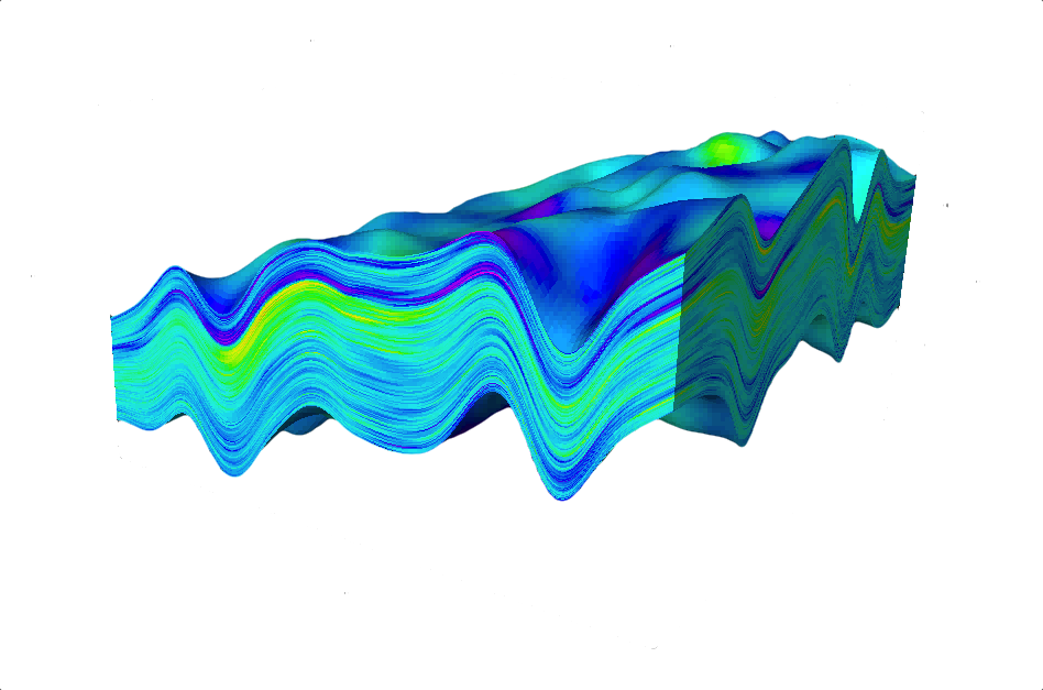
Figure 1: Realization of an oil reservoir by SPECTRAL.

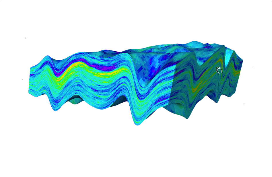
Figure 2: Realization of an oil reservoir by SGS.

Here $\mathrm{GL}\,$ (the gamma logging) is the natural radioactivity of formation, and a reservoir is modeled as the excursion set $\{\alpha\mathrm{GL}\,\leq\mathrm{const}\,\}$ of the function

$$\alpha\mathrm{GL}\,=\frac{\mathrm{GL}\,-\mathrm{GL}\,_{\min}}{\mathrm{GL}\,_{\max}-\mathrm{GL}\,_{\min}},$$

defined on the cube of size $120\times 120\times 490$. We note that we have the reverse inequality in the definition of an excursion because the permeability of a formation is inverse to its radioactivity. In Fig. 3 and Fig. 4 there are displayed the excursion sets $\{\alpha\Gamma K\leq 0.6\}$ for the two realizations given in Fig. 1 and Fig. 2. Different colors correspond to different connected components.

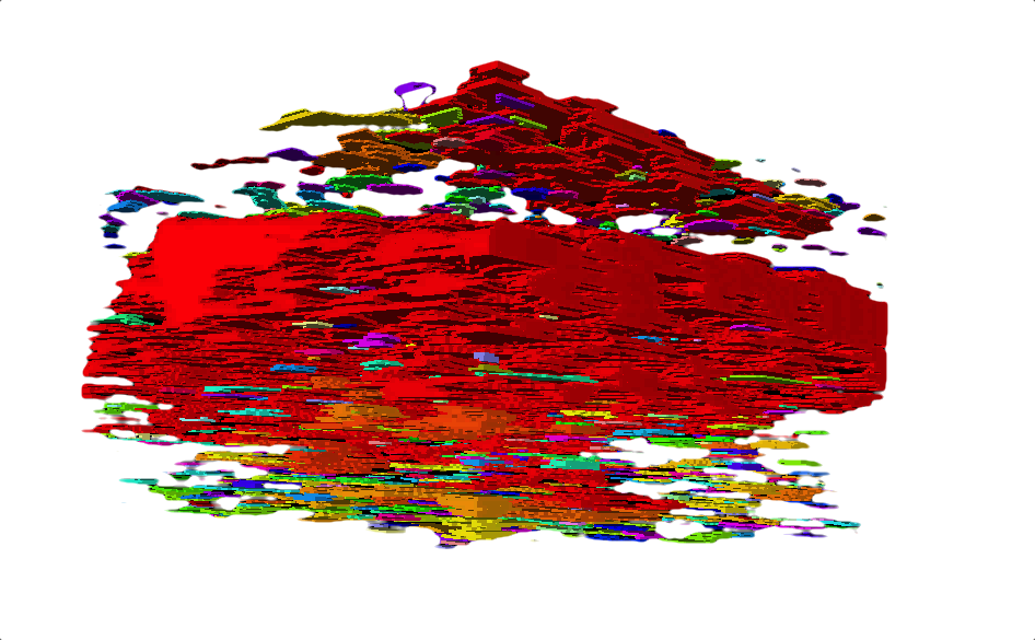
Figure 3: Excursion of a realization of oil reservoir obtained by SPECTRAL.

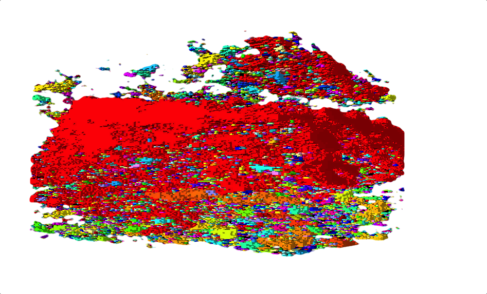
Figure 4: Excursion of a realization of oil reservoir obtained by SGS.

For every realization the Betti numbers and the Euler characteristic $\chi=b_{0}-b_{1}+b_{2}$ are computed. Table 1 demonstrates the dependence of the Betti numbers and the Euler characteristic on the excursion level. For every excursion level we give results of computing the topological characteristics of two different models of the same reservoir that are obtained by the method SPECTRAL (the upper line) and by the SGS method (the lower line). The last column contains the duration of computations on the processor Intel®Core™i7 3.33GHz. In Fig. 5–8 one may find graphs of different characteristics of excursion for both methods. We note that Betti numbers may distinguish the models of reservoirs obtained by the different methods of geostochastic modeling from the same geophysical data.

$\alpha\mbox{ }\mbox{ }$	b0	b1	b2	$\chi$	Time (hr:min:sec)
0.2	19085	72	0	19013	00:00:07
	50874	252	3	50625	00:00:12
0.3	30647	567	3	30083	00:00:24
	78291	2634	29	75686	00:00:41
0.4	40420	3977	34	36446	00:00:52
	98672	13162	298	85808	00:03:31
0.5	46029	10934	196	44291	00:02:34
	104647	31758	1287	74176	00:13:58
0.6	39377	24800	1167	15744	00:08:15
	88255	65012	4471	27714	00:37:23
0.7	18563	62533	5136	-38834	00:33:20
	43630	143720	15785	-84305	01:41:54
0.8	3106	87319	23308	-60905	00:29:57
	8854	200174	54334	-136986	01:37:07
0.9	174	46653	41312	-5167	00:06:28
	577	122147	97657	-23913	00:20:43
1.0	4	15318	31022	15708	00:01:47
	26	38288	76722	38460	00:01:47

Table 1: The Betti numbers and the Euler characteristic.

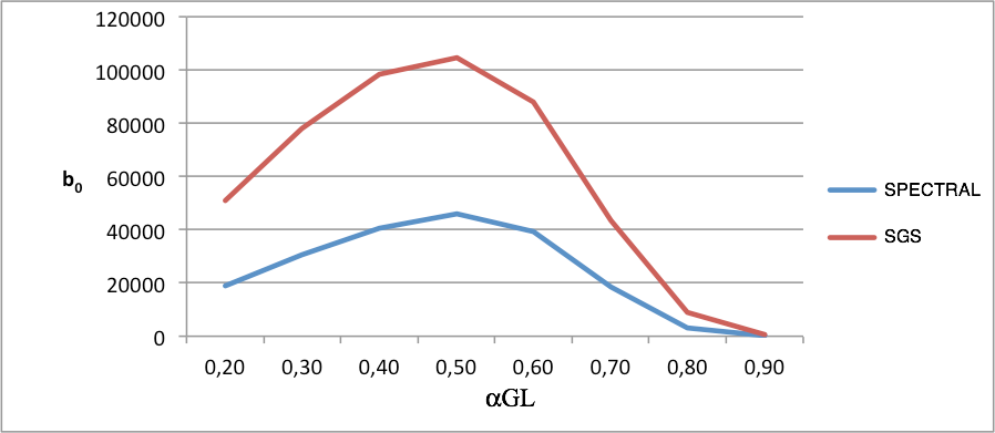
Figure 5: The $0$-th Betti number.

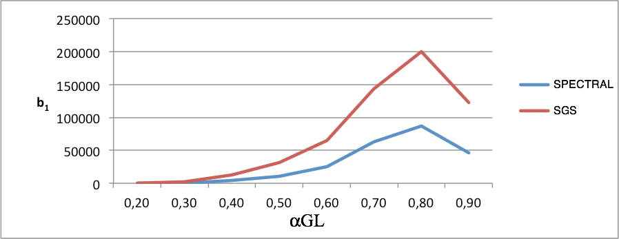
Figure 6: The $1$-st Betti number.

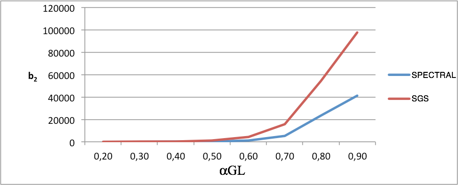
Figure 7: The $2$-nd Betti number.

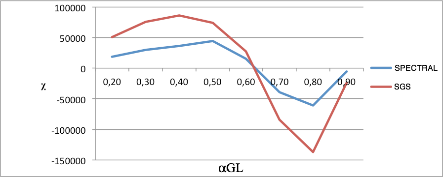
Figure 8: The Euler characteristic.

Remark. A computation of topological characteristics demonstrates the difference between the methods of geostochastical modeling, i.e. between SGS and SPECTRAL: the Betti numbers for different models of the same reservoir may vary upto $2-6$ times.

3 Persistent homology

Rigorous exposition is given, for instance, in [22, 23] of cell complexes and the basic ideas and constructions of Morse theory that we use in the sequel.

For computing the topological characteristics of a space it is convenient to represent the space as a union of elementary “bricks,” i.e. cells, which are “correctly” glued to each other. The resulted space is called a cell complex. By a $0$-dimensional cell one means a point, and a union of finitely many $0$-dimensional cells forms the $0$-th skeleton $X^{0}$ of a cell complex $X$. Let us consider a family of $1$-dimensional cells, i.e. intervals glued to $X$ so that the ends of the intervals are identified with certain $0$-cells. The resulted space would be the $1$-dimensional skeleton $X^{1}$. We construct the complex $X$ by successively gluing $i$-dimensional discs to $(i-1)$-dimensional sceleta $X^{i-1}$.

For our purposes it is enough to use cubic complexes, i.e. such cell complexes that all $i$-cells are $i$-dimensional cubes are glued to $X^{i-1}$ as follows: every boundary face of a $i$-cell is an $(i-1)$-dimensional cube which is identified with some $(i-1)$ cube from $X^{i-1}$.

Let us consider the filtration of a cell complex $X$ by cell subcomplexes:

$$\emptyset=X_{0}\subset X_{1}\subset\ldots\subset X_{n}=X.$$

We consider homology with coefficients in the residue group ${\mathbb{Z}}_{2}$. The filtration defines the chain of homomorphisms of the homology groups $H_{q}^{p}=H_{q}(X_{p})$:

$$0=H_{q}^{0}\to H_{q}^{1}\to\ldots\to H_{q}^{n}\to H_{q}^{n+1}=0$$

for every $q\geq 0$. The compositions of successive homomorphisms from the chains give rise to the homomorphisms

$$f_{q}^{i,j}:H_{q}^{i}\to H_{q}^{j}.$$

By definition, the persistent homology groups of dimension $q$ are the groups

$$H_{q}^{i,j}=\mathrm{Im}\,f_{q}^{i,j}\ \ \ \mbox{for $0\leq i\leq j\leq n+1$.}$$

Respectively by $q$-th persistent Betti numbers we mean the ranks of the persistent homology groups: $b_{q}^{i,j}=\mathrm{rank}\,H_{q}^{i,j}$. In particular, $H_{q}^{i,i}=H_{q}^{i}$.

Let us fix $q$ and choose a basis $\{e_{1}^{i},e_{2}^{i},\ldots,e_{m_{i}}^{i}\}$ for $H_{q}^{i}$ such that for every $1\leq k\leq m_{i}$, $f_{q}^{i,i+1}(e_{k}^{i})\in\{0,e_{1}^{i+1},\ldots,e_{m_{i+1}}^{i+1}\}$ for every $1\leq k\leq m_{i}$ and $f_{q}^{i,i+1}(e_{k}^{i})=f_{q}^{i,i+1}(e_{k^{\prime}}^{i}),k\neq k^{\prime}$ if and only if $f_{q}^{i,i+1}(e_{k}^{i})=0$. Hence $H_{q}^{i,i+1}$ consists of such elements $e_{k}^{i}$ that do not vanish, i.e. survive. Respectively the persistent homology group $H_{q}^{i,j}$ consists of elements $e_{k}^{i}\in H_{q}^{i}$ that survive up to $H_{q}^{j}$.

There is a useful graphical representation for persistent homology that is called a barcode [9, 10, 13]. Namely, given the dimension $q$, let us consider a basic element $e_{k}^{i}$ that is not an image of any element from $H^{i-1}_{q}$. Then here exists a minimal value $j\geq i$ such that $f_{q}^{i,j}(e_{k}^{i})=0$. Then we correspond to $e_{k}^{i}$ the interval $(i,j)$. A disjoint union of all such intervals is usually portrayed on the two-plane by intervals parallel to the $Ox$ axis and forms the $q$-barcode. It gives a visual representation for changing of topology of $X_{i}$ with increasing of $i$.

4 Computation of homology

In this section we demonstrate the main ideas of the numerical algorithm for computing the Betti numbers of three-dimensional bodies which is presented in [18] by using an example of computing the persistent $0$- and $2$-homology and present some results of computations.

Let us consider some cubic domain, in the Euclidean space,

$$K=[0,N]\times[0,N]\times[0,N]\subset{\mathbb{R}}^{3},$$

with some natural $N$. By an elementary interval $I\subset{\mathbb{R}}$ we mean a set of the form

$$I=[l,l+1],$$

where $l$ is some natural number. Analogously we define natural square

$$Q=I_{1}\times I_{2}\subset{\mathbb{R}}^{2},$$

and elementary cube

$$C=I_{1}\times I_{2}\times I_{3}\subset{\mathbb{R}}^{3},$$

where $I_{k},k=1,2,3$ are elementary intervals. Hence the domain $K$ consists of elementary cubes.

Let $M_{1},\dots,M_{n}$ be $3$-dimensional bodies formed by elementary cubes and lying inside $K$. We assume that every $M_{i}$ is the excursion set $\{f\geq c_{i}\}$ for some continuous function $f$ defined on elementary cubes from $K$ and $c_{i}>c_{j}$ for $i<j$. Hence we have the filtration

$$M_{1}\subset M_{2}\subset\dots\subset M_{n}.$$

Variation of an excursion level from $c_{1}$ to $c_{n}$ results in variation of the topology of the excursion sets and that may be described in terms of the persistent homology $H_{\ast}^{i}=H_{\ast}(M_{i})$.

By applying, if need be, the preprocessing of $M$ [18], we assume that two elementary cubes from $M$ may not touch each other only at a vertex or along an edge. In applications that means that oil may pass from one cell to another only through a common $2$-dimensional face and there is no oil passing through common vertices and edges.

In [18] there is proposed a numerical algorithm for computing the homology groups of $M_{i}$ by using a discrete version of Morse theory. Let us briefly expose the main constructions. We consider the “diagonal” linear function on $K$:

$$f(x_{1},x_{2},x_{3})=x_{1}+x_{2}+x_{3},$$

and the excursion sets

$$M_{i}^{a}=\{\bar{x}\in M_{i}|f(\bar{x})\leq a\}.$$

A critical point of $f$ is a vertex $v\in M_{i}$, i.e. an integer-valued point of the rectangular lattice in $K$, such that when $a$ passes $af(v)$ the topology of $M_{i}^{a}$ changes. All combinatorial types of critical points $v=(k_{1},k_{2},k_{3})$ are classified in terms of their elementary neighborhoods:

$$N(v)=\{\bar{x}\in M||x_{i}-k_{i}|\leq 1,i=1,2,3\}.$$

A nondegenerate critical point has index $0$, $1$, or $2$ being the dimension of a cell that glued to $M_{i}^{a}$ when $a$ passes the critical level. Moreover, there is a degenerate critical point, the “monkey saddle,” such that two $1$-dimensional cells are glued during passing the corresponding critical level. In Fig. 9 and Fig. 10 there are exposed the classical critical points: the saddle defined by the equation $f(x,y)=x^{2}-y^{2})$ and the “monkey saddle,” defined by the equation $f(x,y)=x^{3}-xy^{2}$, and also their discrete analogs.

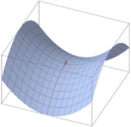
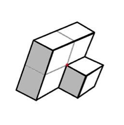
Figure 9: The saddle and its discrete analog.

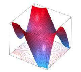
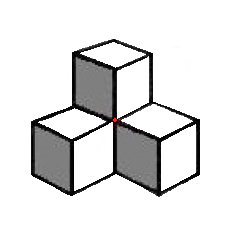
Figure 10: The “monkey saddle” and its discrete analog.

In [18] it is constructed a chain complex

$$C_{2}(M_{i})\to C_{1}(M_{i})\to C_{0}(M_{i}),$$

consisting of vector spaces $C_{q}(M_{i})$ over ${\mathbb{Z}}_{2}$. The basic vectors in $C_{q}(M_{i})$ correspond to the critical points of index $q$ and, moreover, the monkey saddle correspond to a pair of basic vectors from $C_{1}(M_{i})$: to each monkey saddle $v$ we add a fictive vertex $v^{\prime}$ which lies above $v$ with respect to the level of $f$ and a fictive edge $vv^{\prime}$ that joins $v$ and $v^{\prime}$). The horizontal arrows denote the differentials, i.e. linear operators $\partial_{2}^{i}:C_{2}(M_{i})\to C_{1}(M_{i})$ and $\partial_{1}^{i}:C_{1}(M_{i})\to C_{0}(M_{i})$ such that $\mathrm{Ker}\,\partial^{i}_{1}=\mathrm{Im}\,\partial^{i}_{2}$. We have

$$B_{q}=\mathrm{Im}\,\{C_{q+1}\to C_{q}\},\ \ Z_{q}=\mathrm{Ker}\,\{C_{q}\to C_{q-1}\},\ \ H_{q}=Z_{q}/B_{q}$$

where we assume that $C_{3}=C_{-1}=0$.

The differentials are constructed explicitly [18] and for a demonstrative example we need only the following property:

If $v$ is a critical point of index $1$, then there is a pair of sequences of vertices $L(v)=[(v,v_{1}^{-},\ldots,v_{k}^{-})$, $(v,v_{1}^{+},\ldots,v_{m}^{+})]$ such that they contain exactly two critical points of index $0$ which are $v_{k}^{-}$ and $v_{m}^{+}$ and every two consecutive points $v_{i}^{-},v_{i+1}^{-}$ or $v_{i}^{+},v_{i+1}^{+}$ are connected by a negative edge, i.e. such an edge that the value of $f$ at its end is less that at its starting point. Then $\partial_{1}(v)=v_{k}^{-}+v_{m}^{+}$.

Our task is to construct the homomorphisms $\varphi_{q}^{i}:C_{q}(M_{i})\to C_{q}(M_{i+1})$ compatible with differentials. After that, as explained in the previous section, we can calculate the persistent homology and construct the barcodes that reflect the dynamics of change of the topological structure of a $M_{i}$ as $i$ increases. Immediately we understand the arising difficulty: the natural inclusion $M_{i}\subset M_{i+1}$ induces no the natural homomorphism $\varphi_{q}^{i}:C_{q}(M_{i})\to C_{q}(M_{i+1})$ at the critical points, and so there are no natural homomorphisms of homology groups induced by the embedding $M_{i}\subset M_{i+1}$. This difficulty is overcomed by the use of the discrete gradient flow similar to that which was introduced in [18].

First we define the gradient descent of an arbitrary graph $\Gamma$ formed by edges. Namely we assume that $\Gamma^{\prime}$ is obtained by an elementary descent of $\Gamma$, if 1) $(\Gamma\setminus\Gamma^{\prime})\cup(\Gamma^{\prime}\setminus\Gamma)$ is the boundary (possibly without vertices) of the elementary face, and 2) all the vertices of $\Gamma^{\prime}\setminus\Gamma$ lie on the lower levels of $f$ than all the vertices of $\Gamma\setminus\Gamma^{\prime}$ and $\Gamma^{\prime}\setminus\Gamma$ is not empty. If $\Gamma^{\prime}$ is obtained from $\Gamma$ by a finite sequence of elementary descents and there is no elementary descent for $\Gamma^{\prime}$, then we say that $\Gamma^{\prime}$ is obtained from $\Gamma$ by gradient descent.

Next we assume that we have a pair of three-dimensional bodies $M\subset N$, consisting of elementary cubes. It suffices to construct homomorphisms of chain groups for such pairs. Let $M_{q}$ and $N_{q}$ be the sets of critical points, of index $q$, of $f$ in $M$ and in $N$. Let $v\in M_{0}$. Given $v\in N_{0}$ put $\varphi_{0}(v)=v$. Otherwise, there is a negative edge $e_{1}$, in $N$, starting at $v$, and let $v_{1}$ be its another end. If $v_{1}\in N_{0}$, then we put $\varphi_{0}(v)=v_{1}$, and etc. We obtain an iterative process that results in the chain $\Phi(v)=(v,v_{1},\ldots,v_{k})$, where $v\in M_{0}$, $v_{k}\in N_{0}$, $v_{i}\notin N_{0}$ for $1\leq i<k$, and all edges $[v_{i},v_{i+1}]$ are negative. We put $\varphi_{0}(v)=v_{k}$.

Let $v\in M_{1}$. Let us construct $L_{M}(v)=[(v,v_{1}^{-},\ldots,v_{k}^{-}),(v,v_{1}^{+},\ldots,v_{m}^{+})]$. To each of the sequences from $L_{M}(v)$, we add the sequence $\Phi(v_{k}^{-})$ or $\Phi(v_{m}^{+})$, respectively, and obtain a new pair of sequences $[(v,\ldots,v_{k}^{-},\ldots,v_{p}^{-})$, $(v,\ldots,$ $v_{m}^{+},\ldots,v_{q}^{+})]$. Let us construct the graph $\Gamma$ consisting of the edges $[v_{i}^{-},v_{i+1}^{-}]$, $[v_{i}^{+},v_{i+1}^{+}]$, $1\leq i\leq k-1$, and $[v,v_{1}^{-}]$, $[v,v_{1}^{+}]$ and let $\Gamma^{\prime}$ be obtained from $\Gamma$ by the gradient descent. Obviously, the vertices $v_{p}^{-}$ and $v_{q}^{+}\in N_{0}$ and their constituent edges cannot down below. Therefore there exists a path $\gamma^{\prime}$ in $\Gamma^{\prime}$ which connects $v_{p}^{-}$ and $v_{q}^{+}$. Let us consider all critical points $w_{1},\ldots,w_{l}$ of index $1$ in $\gamma^{\prime}$ and put $\varphi_{1}(v)=\sum\limits_{i=1}^{l}w_{i}$.

We have $\varphi_{0}(\partial_{1}(v))=\varphi_{0}(v_{k}^{-}+v_{m}^{+})=v_{p}^{-}+v_{q}^{+}$ for $v\in M_{1}$. But $\partial_{1}(\varphi_{1}(v))=\partial_{1}(\sum\limits_{i=1}^{l}{w_{i}})$. Since the expansions for $\partial_{1}(w_{i})$ and for $\partial_{1}(w_{i+1})$ have a common component that is a critical point of index $0$ and the field of coefficients is of characteristic $2$, $\partial_{1}(\varphi_{1}(v))=v_{p}^{-}+v_{q}^{+}$. Hence $\varphi_{0}(\partial_{1}(v))=\partial_{1}(\varphi_{1}(v))$, i.e. the differentials commute with the homomorphisms og homology groups induced by the embeddings.

The commutative diagram

$$\begin{array}[]{ccccc}&C_{1}(M)&\stackrel{{\scriptstyle\varphi_{1}}}{{\longrightarrow}}&C_{1}(N)&\\ \partial_{1}&\downarrow&&\downarrow&\partial_{1}\\ &C_{0}(M)&\stackrel{{\scriptstyle\varphi_{0}}}{{\longrightarrow}}&C_{0}(N)&\end{array}$$

enables us to compute the persistent $0$-homology.

To compute the persistent $2$-homology we have to use duality [18] and to compute the persistent $0$-homology for the dual space. Namely, let us consider the three-dimensional body $M^{\prime}=K\setminus M$, the complement to $M$, and the function $h=-f$. Clearly the critical points of indices $0$, $1$, and $2$ of $h$ coincide with the critical points of indices $2$, $1$, and $0$ of $f$ and so we may reduce the computation of $2$-homology and $2$-barcodes of $M$ to the computation of $0$-homology and $0$-barcodes of $M^{\prime}$.

In Fig. 11 we present the barcodes of persistent $2$-homology of reservoirs obtained by SPECTRAL (above) and SGS (below).

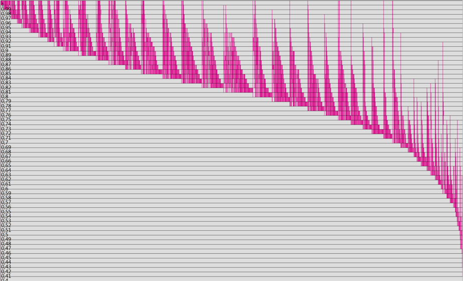
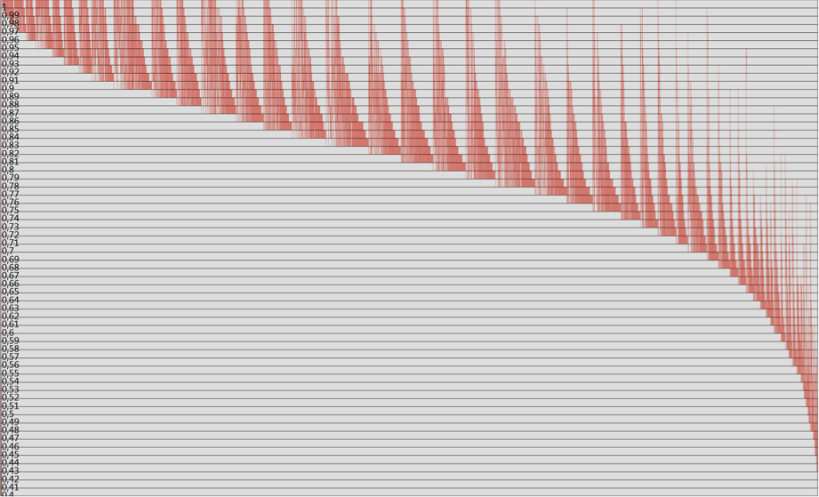
Figure 11: 2-barcodes of the realizations obtained by SPECTRAL (above) and SGS (below). The excursion level values are plotted along the vertical.

References

- [1] Baikov, V.A., Bochkov, A.S., and Yakovlev, A.A.: The heterogeneuity of the Priobskoye field geological modeling and simulation. Oil Industry (2011), N. 5, 50–54. [Russian]
- [2] Baikov, V.A., and Yakovlev, A.A.: Reproduction of geological heterogeneity in geological and hydrodynamic models. Rosneft Scientific and Technical Bulletin (2010), N. 2, 13–15. [Russian]
- [3] Baikov, V.A., Bezrukov, A.V., Bikbulatov, S.M., Emchenko, O.V., Mukharlyamov, A.R., Suleimanov, D.D., and Usmanov, T.S.: A use of normal well development data for elimination of geostatistical modeling uncertainties. Oil Industry (2009), N. 11, 16–19. [Russian]
- [4] Baikov, V.A., Emchenko, O.V., Roschektaev, A.P., and Yakovlev, A.A.: Geological multifactor simulation exemplified by the Priobskoye field. CKR Rosnedra Bulletin (2010), N. 1, 27–34. [Russian]
- [5] Edelsbrunner, H.: Geometry and Topology for Mesh Generation. Cambridge University Press, Cambridge, 2001.
- [6] Kaczynski, T., Mischaikow, K., and Mrozek, M.: Computational Homology. Appl. Math. Sci. Series 157, Springer-Verlag, New York, 2004.
- [7] Zomorodian, A.J.: Topology for Computing. Cambridge University Press, Cambridge, 2005.
- [8] Edelsbrunner, H., Letscher, D., and Zomorodian, A.: Topological persistence and simplification. Discrete Comput. Geom. 28 (2002), 511–533.
- [9] Zomorodian, A., and Carlsson, G.: Computing persistent homology. Discrete Comput. Geom. 33 (2005), 249–274.
- [10] Cohen-Steiner, D., Edelsbrunner, H., and Harer, J.: Stability of persistence diagrams, in: Proc. 21st Sympos. Comput. Geom. (2005), 263–271.
- [11] Bubenik P., and Kim, P.T.: A statistical approach to persistent homology. Homology, Homotopy and Applications 9 (2007), 337–362.
- [12] Edelsbrunner, H., and Harer, J.: Persistent homology — a survey. In: Surveys on discrete and computational geometry. Contemp. Math. 453, Amer. Math. Soc., Providence, RI, 2008, pp. 257–282.
- [13] Ghrist R.. Barcodes: The persistent topology of data. Bull. Amer. Math. Soc. 45 (2008), 61–75.
- [14] Carlsson G.: Topology and data. Bull. Amer. Math. Soc. 46 (2009), 255–308.
- [15] Carlsson, G., and Zomorodian, A.: The theory of multidimensional persistence. Discrete Comput. Geom. 42 (2009), 71–93.
- [16] Adler, R.J., Bobrowski, O., Borman, M.S., Subag, E., and Weinberger, S.: Persistent Homology for Random Fields and Complexes. In: Borrowing strength: theory powering applications – a Festschrift for Lawrence D. Brown, 124–143, Inst. Math. Stat. Collect., 6, Inst. Math. Statist., Beachwood, OH, 2010.
- [17] Adler, R.J., and Taylor, J.E.: Random Fields and Geometry. Springer Monographs in Mathematics, Springer, New York, 2007.
- [18] Bazaikin, Ya.V., and Taimanov, I.A.: On a numerical algorithm for computing topological characteristics of three-dimensional bodies. J. of Comp. Math. and Math. Phys. 2013 (to appear) [Russian]; arXiv:1302.3669.
- [19] Deutsch, C.V., and Journel, A.G.: GSLIB, Geostatistical Software Library and User’s Guide. Oxford University Press, New York, 1992.
- [20] Baikov, V.A., Bakirov, N.K., and Yakovlev, A.A.: New approaches in geostatistical modeling theory. Vestnik UGATU 37:2 (2010), 209–215. [Russian]
- [21] Baikov, V.A., Bakirov, N.K., and Yakovlev, A.A.: New approaches to the geological and hydrodynamic modeling. Oil Industry (2010), N. 9, 56–59. [Russian]
- [22] Seifert, H., and Threlfall, W.: Variationsrechnung im Grossen, AMS Chelsea Publishing, Providence, R.I., 1971.
- [23] Dubrovin, B.A., Fomenko, A.T., and Novikov, S.P.: Modern Geometry - Methods and Applications: Part III: Introduction to Homology Theory. Graduate Texts in Mathematics, 124. Springer, New York, 1990.