Interplay between superconductivity and pseudogap state in bilayer cuprate superconductors

Abstract

The interplay between the superconducting gap and normal-state pseudogap in the bilayer cuprate superconductors is studied based on the kinetic energy driven superconducting mechanism. It is shown that the charge carrier interaction directly from the interlayer coherent hopping in the kinetic energy by exchanging spin excitations does not provide the contribution to the normal-state pseudogap in the particle-hole channel and superconducting gap in the particle-particle channel, while only the charge carrier interaction directly from the intralayer hopping in the kinetic energy by exchanging spin excitations induces the normal-state pseudogap in the particle-hole channel and superconducting gap in the particle-particle channel, and then the two-gap behavior is a universal feature for the single layer and bilayer cuprate superconductors.

The conventional superconductors are characterized by the energy gap, which exists in the excitation spectrum below the superconducting (SC) transition temperature $T_{\rm c}$, and therefore is corresponding to the energy for breaking a Cooper pair of the charge carriers and creating two quasiparticles schrieffer83 . However, in the cuprate superconductors, an energy gap called the normal-state pseudogap exists Hufner08 ; Timusk99 above $T_{\rm c}$ but below the pseudogap crossover temperature $T^{*}$, which is associated with some anomalous properties. Although the charge carrier pair gap in the cuprate superconductors has a domelike shape of the doping dependence damascelli03 ; campuzano04 , the magnitude of the normal-state pseudogap is much larger than that of the charge carrier pair gap in the underdoped regime Hufner08 ; Timusk99 , then it smoothly decreases upon increasing doping, and seems to merge with the charge carrier pair gap in the overdoped regime, eventually disappearing together with superconductivity at the end of the SC dome Hufner08 . In this case, the charge carrier pair gap and normal-state pseudogap are thus two fundamental parameters of the cuprate superconductors whose variation as a function of doping and temperature provides important information crucial to understanding the details of superconductivity Hufner08 ; Timusk99 .

Experimentally, a large body of experimental data obtained by using different measurement techniques have provided rather detailed information on the low-energy excitations of the single layer and bilayer cuprate superconductors Hufner08 ; Timusk99 ; damascelli03 ; campuzano04 , where the Bogoliubov-quasiparticle nature of the low-energy excitations is unambiguously established campuzano03 . However, there are numerous anomalies for the bilayer cuprate superconductors damascelli03 ; campuzano04 , which complicate the physical properties of the low-energy excitations in the bilayer cuprate superconductors. This follows a fact that the bilayer splitting (BS) has been observed in the bilayer cuprate superconductors in a wide doping range dfeng01 , which derives the low-energy excitation spectrum into the bonding and antibonding components due to the presence of the bilayer blocks in the unit cell. In particular, it has been argued that this BS may play an important role in the form of the well pronounced peak-dip-hump structure in the low-energy excitation spectrum of the bilayer cuprate superconductors lan07 ; kordyuk02 ; borisenko03 . In this case, an important issue is whether the behavior of the normal-state pseudogap observed in the low-energy excitation spectrum as a suppression of the spectral weight is universal or not. Within the framework of the kinetic energy driven SC mechanism feng0306 , the interplay between the SC gap and normal-state pseudogap in the single layer cuprate superconductors has been studied recently feng12 , where the interaction between charge carriers and spins directly from the kinetic energy by exchanging spin excitations induces the normal-state pseudogap state in the particle-hole channel and SC-state in the particle-particle channel, then there is a coexistence of the SC gap and normal-state pseudogap in the whole SC dome. In particular, this normal-state pseudogap is closely related to the quasiparticle coherent weight, and both the normal-state pseudogap and SC gap are dominated by one energy scale. In this paper, we study the interplay between the SC gap and normal-state pseudogap in the bilayer cuprate superconductors along with this line. We show explicitly that the weak charge carrier interaction directly from the interlayer coherent hopping in the kinetic energy by exchanging spin excitations does not provide the contribution to the normal-state pseudogap in the particle-hole channel and SC gap in the particle-particle channel, while only the strong charge carrier interaction directly from the intralayer hopping in the kinetic energy by exchanging spin excitations induces the normal-state pseudogap in the particle-hole channel and SC gap in the particle-particle channel, and then the two-gap behavior is a universal feature for the single layer and bilayer cuprate superconductors.

The single common feature in the layered crystal structure of the cuprate superconductors is the presence of the two-dimensional CuO₂ plane damascelli03 , and then it is believed that the unconventional physics properties of the cuprate superconductors is closely related to the doped CuO₂ planes anderson87 . In this case, it is commonly accepted that the essential physics of the doped CuO₂ plane anderson87 is captured by the $t$-$J$ model on a square lattice. However, for discussions of the interplay between the SC gap and normal-state pseudogap in the bilayer cuprate superconductors, the $t$-$J$ model can be extended by including the bilayer interaction as lan07 ,

$$H = -t\sum_{i\hat{\eta}a\sigma}C^{\dagger}_{ia\sigma}C_{i+\hat{\eta}a\sigma}+t^{\prime}\sum_{i\hat{\tau}a\sigma}C^{\dagger}_{ia\sigma}C_{i+\hat{\tau}a\sigma}$$ (1)

$$-\sum_{i\sigma}t_{\perp}(i)(C^{\dagger}_{i1\sigma}C_{i2\sigma}+H.c.)+\mu\sum_{ia\sigma}C^{\dagger}_{ia\sigma}C_{ia\sigma}$$

$$+J\sum_{i\hat{\eta}a}{\bf S}_{ia}\cdot{\bf S}_{i+\hat{\eta}a}+J_{\perp}\sum_{i}{\bf S}_{i1}\cdot{\bf S}_{i2},$$

supplemented by the local constraint $\sum_{\sigma}C_{ia\sigma}^{\dagger}C_{ia\sigma}\leq 1$ to remove double occupancy, where $a=1,2$ is plane index, the summation within the plane is over all sites $i$, and for each $i$, over its nearest-neighbors $\hat{\eta}$ or the next nearest-neighbors $\hat{\tau}$, $C^{\dagger}_{ia\sigma}$ and $C_{ia\sigma}$ are electron operators that respectively create and annihilate electrons with spin $\sigma$, ${\bf S}_{i}=(S^{x}_{i},S^{y}_{i},S^{z}_{i})$ are spin operators, $\mu$ is the chemical potential, while the interlayer hopping has the form in the momentum space,

$$t_{\perp}({\bf k})={t_{\perp}\over 4}(\cos k_{x}-\cos k_{y})^{2},$$ (2)

which describes coherent hopping between the CuO₂ planes. This functional form of the interlayer hopping (2) is predicted on the basis of the local density approximation calculations chakarvarty95 , and later the experimental observed BS agrees well with it dfeng01 . In this bilayer $t$-$J$ model (1), the crucial requirement is to impose the electron single occupancy local constraint, which can be treated properly in analytical calculations within the charge-spin separation (CSS) fermion-spin theory feng04 ; feng08 , where the constrained electron operators are decoupled as $C_{ia\uparrow}=h^{\dagger}_{ia\uparrow}S^{-}_{ia}$ and $C_{ia\downarrow}=h^{\dagger}_{ia\downarrow}S^{+}_{ia}$, with the spinful fermion operator $h_{ia\sigma}=e^{-i\Phi_{ia\sigma}}h_{ia}$ that represents the charge degree of freedom together with some effects of the spin configuration rearrangements due to the presence of the doped hole itself (charge carrier), while the spin operator $S_{ia}$ describes the spin degree of freedom, then the electron single occupancy local constraint is satisfied in analytical calculations. In this CSS fermion-spin representation, the bilayer $t$-$J$ model (1) can be expressed as,

$$H = t\sum_{i\hat{\eta}a}(h^{\dagger}_{i+\hat{\eta}a\uparrow}h_{ia\uparrow}S^{+}_{ia}S^{-}_{i+\hat{\eta}a}+h^{\dagger}_{i+\hat{\eta}a\downarrow}h_{ia\downarrow}S^{-}_{ia}S^{+}_{i+\hat{\eta}a})$$ (3)

$$-t^{\prime}\sum_{i\hat{\tau}a}(h^{\dagger}_{i+\hat{\tau}a\uparrow}h_{ia\uparrow}S^{+}_{ia}S^{-}_{i+\hat{\tau}a}+h^{\dagger}_{i+\hat{\tau}a\downarrow}h_{ia\downarrow}S^{-}_{ia}S^{+}_{i+\hat{\tau}a})$$

$$+\sum_{i}t_{\perp}(i)(h^{\dagger}_{i2\uparrow}h_{i1\uparrow}S^{+}_{i1}S^{-}_{i2}+h^{\dagger}_{i1\uparrow}h_{i2\uparrow}S^{+}_{i2}S^{-}_{i1}$$

$$+h^{\dagger}_{i2\downarrow}h_{i1\downarrow}S^{-}_{i1}S^{+}_{i2}+h^{\dagger}_{i1\downarrow}h_{i2\downarrow}S^{-}_{i2}S^{+}_{i1})-\mu\sum_{ia\sigma}h^{\dagger}_{ia\sigma}h_{ia\sigma}$$

$$+{J_{\rm eff}}\sum_{i\hat{\eta}a}{\bf S}_{ia}\cdot{\bf S}_{i+\hat{\eta}a}+{J_{\rm eff\perp}}\sum_{i}{\bf S}_{i1}\cdot{\bf S}_{i2},$$

where $J_{\rm eff}=J(1-\delta)^{2}$, $J_{\rm eff\perp}=J_{\perp}(1-\delta)^{2}$, and $\delta=\langle h^{\dagger}_{ia\sigma}h_{ia\sigma}\rangle=\langle h^{\dagger}_{ia}h_{ia}\rangle$ is the doping concentration.

For the bilayer cuprate superconductors, there are two coupled CuO₂ planes in one unit cell. In this case, the SC order parameter for the electron Cooper pair is a matrix lan07 $\Delta=\Delta_{\rm L}+\sigma_{x}\Delta_{\rm T}$, with $\Delta_{\rm L}$ and $\Delta_{\rm T}$ are the corresponding longitudinal and transverse parts, respectively. In the doped regime without an antiferromagnetic long-range order (AFLRO), the charge carriers move in the background of the disordered spin liquid state, and then the longitudinal and transverse SC order parameters can be expressed in the CSS fermion-spin representation as, $\Delta_{\rm L}=-\chi_{1}\Delta_{\rm hL}$ and $\Delta_{\rm T}=-\chi_{\perp}\Delta_{\rm hT}$, with

$$\Delta_{\rm hL} = \langle h_{i+\hat{\eta}a\downarrow}h_{ia\uparrow}-h_{i+\hat{\eta}a\uparrow}h_{ia\downarrow}\rangle,$$ (4a)

$$\Delta_{\rm hT} = \langle h_{i2\downarrow}h_{i1\uparrow}-h_{i2\uparrow}h_{i1\downarrow}\rangle,$$ (4b)

are the corresponding longitudinal and transverse parts of the charge carrier pair gap parameter, respectively, and the spin correlation functions $\langle S^{+}_{ia}S^{-}_{i+\hat{\eta}a}\rangle=\langle S^{-}_{ia}S^{+}_{i+\hat{\eta}a}\rangle=\chi_{1}$ and $\langle S^{+}_{i1}S^{-}_{i2}\rangle=\langle S^{-}_{i1}S^{+}_{i2}\rangle=\chi_{\perp}$. The result in Eq. (4) shows that as in the single layer case feng0306 , the SC gap parameter in the bilayer cuprate superconductors is also closely related to the corresponding charge carrier pair gap parameter, and therefore the essential physics in the SC-state is dominated by the corresponding one in the charge carrier pairing state.

Within the framework of the kinetic energy driven SC mechanism feng0306 , the electronic structure of the bilayer cuprate superconductors has been discussed lan07 ; feng08 , and the result shows that the low-energy excitation spectrum is split into the bonding and antibonding components due to the presence of BS, then the observed peak-dip-hump structure is mainly caused by BS, with the peak being related to the antibonding component, and the hump being formed by the bonding component. Following our previous discussions lan07 ; feng08 , the self-consistent equations that satisfied by the full charge carrier normal and anomalous Green’s functions are obtained as,

$$g({\bf k},\omega) = g^{(0)}({\bf k},\omega)+g^{(0)}({\bf k},\omega)[\Sigma^{(\rm h)}_{1}({\bf k},\omega)g({\bf k},\omega)$$ (5a)

$$-\Sigma^{(\rm h)}_{2}(-{\bf k},-\omega)\Im^{\dagger}({\bf k},\omega)],$$

$$\Im^{\dagger}({\bf k},\omega) = g^{(0)}(-{\bf k},-\omega)[\Sigma^{(\rm h)}_{1}(-{\bf k},-\omega)\Im^{\dagger}(-{\bf k},-\omega)$$ (5b)

$$+\Sigma^{(\rm h)}_{2}(-{\bf k},-\omega)g({\bf k},\omega)],$$

respectively, where the full charge carrier normal Green’s function $g({\bf k},\omega)=g_{\rm L}({\bf k},\omega)+\sigma_{x}g_{\rm T}({\bf k},\omega)$, the full charge carrier anomalous Green’s function $\Im^{\dagger}({\bf k},\omega)=\Im^{\dagger}_{\rm L}({\bf k},\omega)+\sigma_{x}\Im^{\dagger}_{\rm T}({\bf k},\omega)$, the charge carrier self-energies $\Sigma^{(\rm h)}_{1}({\bf k},\omega)=\Sigma^{(\rm h)}_{\rm 1L}({\bf k},\omega)+\sigma_{x}\Sigma^{(\rm h)}_{\rm 1T}({\bf k},\omega)$ and $\Sigma^{(\rm h)}_{2}({\bf k},\omega)=\Sigma^{(\rm h)}_{\rm 2L}({\bf k},\omega)+\sigma_{x}\Sigma^{(\rm h)}_{\rm 2T}({\bf k},\omega)$ in the particle-hole and particle-particle channels, respectively, while the mean-field (MF) charge carrier normal Green’s function $g^{(0)}({\bf k},\omega)=g^{(0)}_{\rm L}({\bf k},\omega)+\sigma_{x}g^{(0)}_{\rm T}({\bf k},\omega)$, with the corresponding longitudinal and transverse parts have been obtained as lan07 ; feng08 ,

$$g^{(0)}_{\rm L}({\bf k},\omega) = {1\over 2}\sum_{\alpha=1,2}{1\over\omega-\xi_{\alpha{\bf k}}},$$ (6a)

$$g^{(0)}_{\rm T}({\bf k},\omega) = {1\over 2}\sum_{\alpha=1,2}(-1)^{\alpha+1}{1\over\omega-\xi_{\alpha{\bf k}}},$$ (6b)

respectively, where $\alpha=1,2$, the MF charge carrier spectrum $\xi_{\alpha{\bf k}}=Zt\chi_{1}\gamma_{\bf k}-Zt^{\prime}\chi_{2}\gamma{{}^{\prime}}_{\bf k}-\mu+(-1)^{\alpha+1}\chi_{\perp}t_{\perp}({\bf k})$, the spin correlation function $\chi_{2}=\langle S_{ia}^{+}S_{i+\hat{\tau}a}^{-}\rangle$, $\gamma_{\bf{k}}=(1/Z)\sum_{\hat{\eta}}{e^{i{\bf k}\cdot{\hat{\eta}}}}$, $\gamma{{}^{\prime}}_{\bf k}=(1/Z)\sum_{\hat{\tau}}{e^{i{\bf k}\cdot{\hat{\tau}}}}$, and $Z$ is the number of the nearest neighbor or next nearest neighbor sites. However, in the bilayer coupling case, the more appropriate classification is in terms of the normal and anomalous Green’s functions within the basis of the bonding and antibonding components, i.e., the full charge carrier normal and anomalous Green’s functions can be rewritten in the bonding-antibonding representation as,

$$g_{\nu}({\bf k},\omega) = g_{\rm L}({\bf k},\omega)+(-1)^{\nu+1}g_{\rm T}({\bf k},\omega),$$ (7a)

$$\Im^{\dagger}_{\nu}({\bf k},\omega) = \Im^{\dagger}_{\rm L}({\bf k},\omega)+(-1)^{\nu+1}\Im^{\dagger}_{\rm T}({\bf k},\omega),$$ (7b)

respectively, where $\nu=1,2$, with $\nu=1$ ($\nu=2$) represents the corresponding bonding (antibonding) component, then the bonding and antibonding components of the self-energies $\Sigma^{(\rm h)}_{1}({\bf k},\omega)$ and $\Sigma^{(\rm h)}_{2}({\bf k},\omega)$ can be obtained from the spin bubble as lan07 ; feng08 ,

$$\Sigma^{(\rm h)}_{1\nu}({\bf k},i\omega_{n})=\Sigma^{(\rm h)}_{\rm 1L}({\bf k},i\omega_{n})+(-1)^{\nu+1}\Sigma^{(\rm h)}_{\rm 1T}({\bf k},i\omega_{n})$$

$$\hskip 14.22636pt={1\over 8N^{2}}\sum_{\bf pq}\sum_{\nu_{1}\nu_{2}\nu_{3}}\Lambda^{\nu\nu_{1}\nu_{2}\nu_{3}}_{{\bf p}+{\bf q}+{\bf k}}{1\over\beta}\sum_{ip_{m}}$$

$$\hskip 22.76228pt\times g_{\nu_{1}}({\bf p}+{\bf k},ip_{m}+i\omega_{n})\Pi_{\nu_{2}\nu_{3}}({\bf p},{\bf q},ip_{m}),$$ (8a)

$$\Sigma^{(\rm h)}_{2\nu}({\bf k},i\omega_{n})=\Sigma^{(\rm h)}_{\rm 2L}({\bf k},i\omega_{n})+(-1)^{\nu+1}\Sigma^{(\rm h)}_{\rm 2T}({\bf k},i\omega_{n})$$

$$\hskip 14.22636pt={1\over 8N^{2}}\sum_{\bf pq}\sum_{\nu_{1}\nu_{2}\nu_{3}}\Lambda^{\nu\nu_{1}\nu_{2}\nu_{3}}_{{\bf p}+{\bf q}+{\bf k}}{1\over\beta}\sum_{ip_{m}}$$

$$\hskip 22.76228pt\times\Im^{{\dagger}}_{\nu_{1}}(-{\bf p}-{\bf k},-ip_{m}-i\omega_{n})\Pi_{\nu_{2}\nu_{3}}({\bf p},{\bf q},ip_{m}),~{}~{}~{}~{}~{}$$ (8b)

respectively, with $\Lambda^{\nu\nu_{1}\nu_{2}\nu_{3}}_{\bf k}=[1+(-1)^{\nu+\nu_{1}+\nu_{2}+\nu_{3}}][Z(t\gamma_{\bf k}-t^{\prime}\gamma^{\prime}_{\bf k})+(-1)^{\nu+\nu_{3}}t_{\perp}({\bf k})]^{2}$, and the spin bubble,

$$\Pi_{\nu_{2}\nu_{3}}({\bf p},{\bf q},ip_{m}) = {1\over\beta}\sum_{iq_{m}}D^{(0)}_{\nu_{2}}({\bf q},iq_{m})$$ (9)

$$\times D^{(0)}_{\nu_{3}}({\bf q}+{\bf p},iq_{m}+ip_{m}),$$

where the MF spin Green’s functions $D^{(0)}_{\nu}({\bf p},ip_{m})=B_{\nu{\bf p}}/[(ip_{m})^{2}-\omega^{2}_{\nu{\bf p}}]$, with the MF spin excitation spectrum $\omega_{\nu{\bf p}}$ and function $B_{\nu{\bf p}}$ have been given in Ref. lan07 ; feng08 .

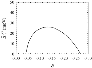
Figure 1: The bonding (solid line) and antibonding (dashed line) components of the effective charge carrier pair gap parameter as a function of doping for temperature $T=0.002J$ with parameters $t/J=2.5$, $t^{\prime}/t=0.3$, $t_{\perp}/t=0.35$ and $J=110$ meV.

As in the single layer case feng0306 , the pairing force and charge carrier pair gap are incorporated into the self-energy $\Sigma^{(\rm h)}_{2\nu}({\bf k},\omega)$, then it is called as the effective charge carrier pair gap $\bar{\Delta}^{(\nu)}_{\rm h}({\bf k},\omega)=\Sigma^{(\rm h)}_{2\nu}({\bf k},\omega)$. On the other hand, the self-energy $\Sigma^{(\rm h)}_{1\nu}({\bf k},\omega)$ renormalizes the MF charge carrier spectrum lan07 ; feng08 . Moreover, $\Sigma^{(\rm h)}_{2\nu}({\bf k},\omega)$ is an even function of $\omega$, while $\Sigma^{(\rm h)}_{1\nu}({\bf k},\omega)$ is not. For a convenience, $\Sigma^{(\rm h)}_{1\nu}({\bf k},\omega)$ can be broken up into its symmetric and antisymmetric parts as, $\Sigma^{(\rm h)}_{1\nu}({\bf k},\omega)=\Sigma^{(\rm h)}_{1\nu{\rm e}}({\bf k},\omega)+\omega\Sigma^{(\rm h)}_{1\nu{\rm o}}({\bf k},\omega)$, then both $\Sigma^{(\rm h)}_{1\nu{\rm e}}({\bf k},\omega)$ and $\Sigma^{(\rm h)}_{1\nu{\rm o}}({\bf k},\omega)$ are an even function of $\omega$. As in the conventional superconductors eliashberg60 , the retarded function ${\rm Re}\Sigma^{(\rm h)}_{1\nu{\rm e}}({\bf k},\omega)$ may be a constant, independent of (${\bf k},\omega$). It just renormalizes the chemical potential, and therefore can be neglected. Now we define the charge carrier coherent weight as $Z^{(\nu)-1}_{\rm hF}({\bf k},\omega)=1-{\rm Re}\Sigma^{(\rm h)}_{1\nu{\rm o}}({\bf k},\omega)$, and then in the static limit approximation, i.e., $Z^{(\nu)-1}_{\rm hF}=1-{\rm Re}\Sigma^{(\rm h)}_{1\nu{\rm o}}({\bf k},\omega=0)\mid_{{\bf k}=[\pi,0]}$, and $\bar{\Delta}^{(\nu)}_{\rm h}({\bf k})=\Sigma^{(\rm h)}_{2\nu}({\bf k},\omega=0)=\Sigma^{(\rm h)}_{\rm 2L}({\bf k},\omega=0)+(-1)^{\nu+1}\Sigma^{(\rm h)}_{\rm 2T}({\bf k},\omega=0)=\bar{\Delta}_{\rm hL}({\bf k})+(-1)^{\nu+1}\bar{\Delta}_{\rm hT}({\bf k})$, with $\bar{\Delta}_{\rm hL}({\bf k})=\bar{\Delta}_{\rm hL}\gamma^{(\rm d)}_{\bf k}$, $\bar{\Delta}_{\rm hT}({\bf k})=\bar{\Delta}_{\rm hT}$, and $\gamma^{(\rm d)}_{\bf k}=({\rm cos}k_{x}-{\rm cos}k_{y})/2$, we lan07 ; feng08 can obtain the full charge carrier normal and anomalous Green’s functions of the bilayer cuprate superconductors. In this case, with the help of these full charge carrier normal and anomalous Green’s functions, the self-energy $\Sigma^{(\rm h)}_{1\nu}({\bf k},\omega)$ and effective charge carrier pair gap $\bar{\Delta}^{(\nu)}_{\rm h}({\bf k})$ in Eq. (8) can be evaluated explicitly as,

$$\Sigma^{(\rm h)}_{1\nu}({\bf k},\omega) = {1\over N^{2}}\sum_{{\bf pq}}\sum_{\nu_{1}\nu_{2}\nu_{3}}\sum_{\sigma_{1}\sigma_{2}\sigma_{3}}\Lambda^{\nu\nu_{1}\nu_{2}\nu_{3}}_{{\bf p}+{\bf q}+{\bf k}}{B_{\nu_{2}{\bf q}}B_{\nu_{3}{\bf q}+{\bf p}}\over 64\omega^{(\sigma_{2})}_{\nu_{2}{\bf q}}\omega^{(\sigma_{3})}_{\nu_{3}{\bf q+p}}}$$ (10a)

$$\times {A_{\sigma_{1}}^{(\nu_{1})}({\bf p}+{\bf k})F_{\sigma_{1}\sigma_{2}\sigma_{3}}^{\nu_{1}\nu_{2}\nu_{3}}({\bf p,q,k})\over\omega-E^{(\sigma_{1})}_{{\rm h}\nu_{1}{\bf p}+{\bf k}}-\omega^{(\sigma_{2})}_{\nu_{2}{\bf q}}+\omega^{(\sigma_{3})}_{\nu_{3}{\bf q}+{\bf p}}},~{}~{}~{}~{}~{}~{}~{}$$

$$\bar{\Delta}^{(\nu)}_{\rm h}({\bf k}) = {1\over N^{2}}\sum_{\bf pq}\sum_{\nu_{1}\nu_{2}\nu_{3}}\sum_{\sigma_{1}\sigma_{2}\sigma_{3}}\Lambda^{\nu\nu_{1}\nu_{2}\nu_{3}}_{{\bf p}+{\bf q}+{\bf k}}{B_{\nu_{2}{\bf q}}B_{\nu_{3}{\bf q}+{\bf p}}\over 64\omega^{(\sigma_{2})}_{\nu_{2}{\bf q}}\omega^{(\sigma_{3})}_{\nu_{3}{\bf q}+{\bf p}}}$$ (10b)

$$\times {\bar{\Delta}_{\rm hZ}^{(\nu_{1})}({\bf p}+{\bf k})\over E^{(\sigma_{1})}_{{\rm h}\nu_{1}{\bf p}+{\bf k}}}{F_{\sigma_{1}\sigma_{2}\sigma_{3}}^{\nu_{1}\nu_{2}\nu_{3}}({\bf p,q,k})\over E^{(\sigma_{1})}_{{\rm h}\nu_{1}{\bf p}+{\bf k}}+\omega^{(\sigma_{2})}_{\nu_{2}{\bf q}}-\omega^{(\sigma_{3})}_{\nu_{3}{\bf q}+{\bf p}}},~{}~{}~{}~{}~{}~{}~{}$$

where $\sigma_{1},\sigma_{2},\sigma_{3}=1,2$, $F_{\sigma_{1}\sigma_{2}\sigma_{3}}^{\nu_{1}\nu_{2}\nu_{3}}({\bf p,q,k})=Z^{(\nu_{1})}_{\rm hF}\{n_{\rm F}(E^{(\sigma_{1})}_{{\rm h}\nu_{1}{\bf p}+{\bf k}})[n_{\rm B}(\omega^{(\sigma_{2})}_{\nu_{2}{\bf q}})-n_{\rm B}(\omega^{(\sigma_{3})}_{\nu_{3}{\bf q}+{\bf p}})]+n_{\rm B}(\omega^{(\sigma_{3})}_{\nu_{3}{\bf q}+{\bf p}})[1+n_{\rm B}(\omega^{(\sigma_{2})}_{\nu_{2}{\bf q}})]\}$, $A_{\sigma_{1}}^{(\nu_{1})}({\bf k})=1+\bar{\xi}_{\nu_{1}\bf k}/E^{(\sigma_{1})}_{{\rm h}\nu_{1}{\bf k}}$, with $\omega^{(1)}_{\nu{\bf p}}=\omega_{{\nu}{\bf p}}$, $\omega^{(2)}_{\nu{\bf p}}=-\omega_{{\nu}{\bf p}}$, $E^{(1)}_{{\rm h}\nu{\bf k}}=E_{{\rm h}\nu{\bf k}}$, $E^{(2)}_{{\rm h}\nu{\bf k}}=-E_{{\rm h}\nu{\bf k}}$, the renormalized charge carrier excitation spectrum $\bar{\xi}_{\nu{\bf k}}=Z^{(\nu)}_{\rm hF}\xi_{\nu{\bf k}}$, the renormalized charge carrier pair gap $\bar{\Delta}_{\rm hZ}^{(\nu)}({\bf k})=Z^{(\nu)}_{\rm hF}\bar{\Delta}^{(\nu)}_{\rm h}({\bf k})$, the charge carrier quasiparticle spectrum $E_{{\rm h}\nu{\bf k}}=\sqrt{{\bar{\xi}}_{\nu{\bf k}}^{2}+\mid\bar{\Delta}_{\rm hZ}^{(\nu)}({\bf k})\mid^{2}}$, and $n_{\rm B}(\omega)$ and $n_{\rm F}(E)$ are the boson and fermion distribution functions, respectively. In particular, the equations $Z^{(\nu)-1}_{\rm hF}=1-{\rm Re}\Sigma^{(\rm h)}_{1\nu{\rm o}}({\bf k},\omega=0)\mid_{{\bf k}=[\pi,0]}$ and $\bar{\Delta}^{(\nu)}_{\rm h}({\bf k})=\Sigma^{(\rm h)}_{2\nu}({\bf k},\omega=0)$ have been solved self-consistently in combination with other equations lan07 ; feng08 , then all order parameters and chemical potential have been obtained by the self-consistent calculation. In Fig. 1, we plot the self-consistently calculated result lan07 of the effective charge carrier pair gap parameter for the bonding $\bar{\Delta}^{(1)}_{\rm h}$ (solid line) and antibonding $\bar{\Delta}^{(2)}_{\rm h}$ (dashed line) components versus the doping concentration in temperature $T=0.002J$ with parameters $t/J=2.5$, $t^{\prime}/t=0.3$, $t_{\perp}/t=0.35$, and $J=110$ meV. It is shown clearly that the maximal $\bar{\Delta}^{(1)}_{\rm h}$ and $\bar{\Delta}^{(2)}_{\rm h}$ occur around the optimal doping, and then decrease in both the underdoped and the overdoped regimes. Moreover, both the bonding and antibonding components of the effective charge carrier pair gap parameter have the same magnitude in a given doping concentration lan07 , which implies the transverse part of the charge carrier pair gap $\bar{\Delta}_{\rm hT}\approx 0$, and then $\bar{\Delta}^{(1)}_{\rm h}\approx\bar{\Delta}^{(2)}_{\rm h}\approx\bar{\Delta}_{\rm hL}$. This result shows that although there is a single electron interlayer coherent hopping (2) in the bilayer cuprate superconductors, the coupling strength for the interlayer pairs vanishes, which reflects that within the framework of the kinetic energy driven SC mechanism, the weak charge carrier interaction directly from the interlayer coherent hopping (2) in the kinetic energy by exchanging spin excitations does not provide any contribution to the charge carrier pair gap in the particle-particle channel, and then the transverse part of the charge carrier pair gap $\bar{\Delta}_{\rm hT}\approx 0$. This is different from the strong charge carrier interaction directly from the intralayer hopping in the kinetic energy by exchanging spin excitations, which induces superconductivity in the particle-particle channel feng0306 , and then the charge carrier pair gap is dominated by the corresponding longitudinal part, i.e., $\bar{\Delta}^{(1)}_{\rm h}\approx\bar{\Delta}^{(2)}_{\rm h}\approx\bar{\Delta}_{\rm hL}$. This result is also consistent with the experimental results of the bilayer cuprate superconductor Bi(Pb)₂Sr₂CaCu₂O_8+δ dfeng01 , where the SC gap separately for the bonding and antibonding components has been measured, and it is found that both the antibonding and bonding components are identical within the experimental uncertainties.

Now we discuss the interplay between the SC-gap and normal-state pseudogap in the bilayer cuprate superconductors. As in the single layer case feng12 , the self-energy $\Sigma^{({\rm h})}_{1}({\bf k},\omega)$ in Eq. (10a) in the particle-hole channel can also be rewritten approximately as,

$$\Sigma^{(\rm h)}_{1}({\bf k},\omega)\approx{[2\bar{\Delta}_{\rm pg}({\bf k})]^{2}\over\omega+M_{\bf k}},$$ (11)

where $M_{\bf k}=M_{{\rm L}{\bf k}}+\sigma_{x}M_{{\rm T}{\bf k}}$ is the energy spectrum of $\Sigma^{(\rm h)}_{1}({\bf k},\omega)$. As in the case of the effective charge carrier pair gap, the interaction force and normal-state pseudogap have been incorporated into $\bar{\Delta}_{\rm pg}({\bf k})=\bar{\Delta}_{\rm pgL}({\bf k})+\sigma_{x}\bar{\Delta}_{\rm pgT}({\bf k})$, and therefore it is called as the effective normal-state pseudogap. In the bonding-antibonding representation, the self-energy in Eq. (11) can be expressed as,

$$\Sigma^{(\rm h)}_{1\nu}({\bf k},\omega)\approx{[2\bar{\Delta}^{(\nu)}_{\rm pg}({\bf k})]^{2}\over\omega+M_{\nu{\bf k}}},$$ (12)

with $M_{\nu{\bf k}}=M_{{\rm L}{\bf k}}+(-1)^{\nu+1}M_{{\rm T}{\bf k}}$, and $\bar{\Delta}^{(\nu)}_{\rm pg}({\bf k})=\bar{\Delta}_{\rm pgL}({\bf k})+(-1)^{\nu+1}\bar{\Delta}_{\rm pgT}({\bf k})$. Substituting $\Sigma^{(\rm h)}_{1\nu}({\bf k},\omega)$ in Eq. (12) into Eq. (5), the full charge carrier normal and anomalous Green’s functions can be obtained straightforwardly as,

$$g_{\nu}({\bf k},\omega) = {1\over\omega-\xi_{\nu{\bf k}}-\Sigma^{(\rm h)}_{1\nu}({\bf k},\omega)-[\bar{\Delta}^{(\nu)}_{\rm h}({\bf k})]^{2}/[\omega+\xi_{\nu{\bf k}}+\Sigma^{(\rm h)}_{1\nu}(-{\bf k},-\omega)]}$$ (13a)

$$= {[U^{(\nu)}_{1{\rm h}{\bf k}}]^{2}\over\omega-E^{(\nu)}_{1{\rm h}{\bf k}}}+{[V^{(\nu)}_{1{\rm h}{\bf k}}]^{2}\over\omega+E^{(\nu)}_{1{\rm h}{\bf k}}}+{[U^{(\nu)}_{2{\rm h}{\bf k}}]^{2}\over\omega-E^{(\nu)}_{2{\rm h}{\bf k}}}+{[V^{(\nu)}_{2{\rm h}{\bf k}}]^{2}\over\omega+E^{(\nu)}_{2{\rm h}{\bf k}}},$$

$$\Im^{\dagger}_{\nu}({\bf k},\omega) = -{\bar{\Delta}^{(\nu)}_{\rm h}({\bf k})\over[\omega-\xi_{\nu{\bf k}}-\Sigma^{(\rm h)}_{1\nu}({\bf k},\omega)][\omega+\xi_{\nu{\bf k}}+\Sigma^{(\rm h)}_{1\nu}(-{\bf k},-\omega)]-[\bar{\Delta}^{(\nu)}_{\rm h}({\bf k})]^{2}}$$ (13b)

$$= -{\alpha^{(\nu)}_{1{\bf k}}\bar{\Delta}^{(\nu)}_{\rm h}({\bf k})\over 2E^{(\nu)}_{1{\rm h}{\bf k}}}\left({1\over\omega-E^{(\nu)}_{1{\rm h}{\bf k}}}-{1\over\omega+E^{(\nu)}_{1{\rm h}{\bf k}}}\right)+{\alpha^{(\nu)}_{2{\bf k}}\bar{\Delta}^{(\nu)}_{\rm h}({\bf k})\over 2E^{(\nu)}_{2{\rm h}{\bf k}}}\left({1\over\omega-E^{(\nu)}_{2{\rm h}{\bf k}}}-{1\over\omega+E^{(\nu)}_{2{\rm h}{\bf k}}}\right),$$

respectively, where $\alpha^{(\nu)}_{1{\bf k}}=\{[E^{(\nu)}_{1{\rm h}{\bf k}}]^{2}-M^{2}_{\nu{\bf k}}\}/\{[E^{(\nu)}_{1{\rm h}{\bf k}}]^{2}-[E^{(\nu)}_{2{\rm h}{\bf k}}]^{2}\}$, $\alpha^{(\nu)}_{2{\bf k}}=\{[E^{(\nu)}_{2{\rm h}{\bf k}}]^{2}-M^{2}_{\nu{\bf k}}\}/\{[E^{(\nu)}_{1{\rm h}{\bf k}}]^{2}-[E^{(\nu)}_{2{\rm h}{\bf k}}]^{2}\}$, $E^{(\nu)}_{1{\rm h}{\bf k}}=\sqrt{(\Omega_{\nu{\bf k}}+\Theta_{\nu{\bf k}})/2}$, and $E^{(\nu)}_{2{\rm h}{\bf k}}=\sqrt{(\Omega_{\nu{\bf k}}-\Theta_{\nu{\bf k}})/2}$, with the kernel functions,

$$\Omega_{\nu{\bf k}} = \xi^{2}_{\nu{\bf k}}+M^{2}_{\nu{\bf k}}+8[\bar{\Delta}^{(\nu)}_{\rm pg}({\bf k})]^{2}+[\bar{\Delta}^{(\nu)}_{\rm h}({\bf k})]^{2},$$ (14a)

$$\Theta_{\nu{\bf k}} = \sqrt{(\xi^{2}_{\nu{\bf k}}-M^{2}_{\nu{\bf k}})\beta^{(\nu)}_{1{\bf k}}+16[\bar{\Delta}^{(\nu)}_{\rm pg}({\bf k})]^{2}\beta^{(\nu)}_{2{\bf k}}+[\bar{\Delta}^{(\nu)}_{\rm h}({\bf k})]^{4}},$$

where $\beta^{(\nu)}_{1{\bf k}}=\xi^{2}_{\nu{\bf k}}-M^{2}_{\nu{\bf k}}+2[\bar{\Delta}^{(\nu)}_{\rm h}({\bf k})]^{2}$, $\beta^{(\nu)}_{2{\bf k}}=(\xi_{\nu{\bf k}}-M_{\nu{\bf k}})^{2}+[\bar{\Delta}^{(\nu)}_{\rm h}({\bf k})]^{2}$, while the coherence factors,

$$(U^{(\nu)}_{1{\rm h}{\bf k}})^{2} = {1\over 2}\{\alpha^{(\nu)}_{1{\bf k}}[1+{\xi_{\nu{\bf k}}\over E^{(\nu)}_{1{\rm h}{\bf k}}}]-\alpha^{(\nu)}_{3{\bf k}}[1+{M_{\nu{\bf k}}\over E^{(\nu)}_{1{\rm h}{\bf k}}}]\},$$ (15a)

$$(V^{(\nu)}_{1{\rm h}{\bf k}})^{2} = {1\over 2}\{\alpha^{(\nu)}_{1{\bf k}}[1-{\xi_{\nu{\bf k}}\over E^{(\nu)}_{1{\rm h}{\bf k}}}]-\alpha^{(\nu)}_{3{\bf k}}[1-{M_{\nu{\bf k}}\over E^{(\nu)}_{1{\rm h}{\bf k}}}]\},$$ (15b)

$$(U^{(\nu)}_{2{\rm h}{\bf k}})^{2} = -{1\over 2}\{\alpha^{(\nu)}_{2{\bf k}}[1+{\xi_{\nu{\bf k}}\over E^{(\nu)}_{2{\rm h}{\bf k}}}]-\alpha^{(\nu)}_{3{\bf k}}[1+{M_{\nu{\bf k}}\over E^{(\nu)}_{2{\rm h}{\bf k}}}]\},$$ (15c)

$$(V^{(\nu)}_{2{\rm h}{\bf k}})^{2} = -{1\over 2}\{\alpha^{(\nu)}_{2{\bf k}}[1-{\xi_{\nu{\bf k}}\over E^{(\nu)}_{2{\rm h}{\bf k}}}]-\alpha^{(\nu)}_{3{\bf k}}[1-{M_{\nu{\bf k}}\over E^{(\nu)}_{2{\rm h}{\bf k}}}]\},~{}~{}~{}~{}~{}~{}~{}$$ (15d)

satisfy the sum rule: $[U^{(\nu)}_{1{\rm h}{\bf k}}]^{2}+[V^{(\nu)}_{1{\rm h}{\bf k}}]^{2}+[U^{(\nu)}_{2{\rm h}{\bf k}}]^{2}+[V^{(\nu)}_{2{\rm h}{\bf k}}]^{2}=1$, with $\alpha^{(\nu)}_{3{\bf k}}=[2\bar{\Delta}^{(\nu)}_{\rm pg}({\bf k})]^{2}/\{[E^{(\nu)}_{1{\rm h}{\bf k}}]^{2}-[E^{(\nu)}_{2{\rm h}{\bf k}}]^{2}\}$, and then the corresponding effective normal-state pseudogap $\bar{\Delta}^{(\nu)}_{\rm pg}({\bf k})$ and energy spectra $M_{\nu{\bf k}}$ can be obtained explicitly in terms of the self-energies $\Sigma^{(\rm h)}_{1\nu}({\bf k},\omega)$ in Eq. (10a) as,

$$\bar{\Delta}^{(\nu)}_{\rm pg}({\bf k}) = {L^{(\nu)}_{2}({\bf k})\over 2\sqrt{L^{(\nu)}_{1}({\bf k})}},$$ (16a)

$$M_{\nu{\bf k}} = {L^{(\nu)}_{2}({\bf k})\over L^{(\nu)}_{1}({\bf k})},$$ (16b)

where $L^{(\nu)}_{1}({\bf k})$ and $L^{(\nu)}_{2}({\bf k})$ are obtained from Eq. (10a) as,

$$L^{(\nu)}_{1}({\bf k}) = {1\over N^{2}}\sum_{{\bf pq}}\sum_{\nu_{1}\nu_{2}\nu_{3}}\sum_{\sigma_{1}\sigma_{2}\sigma_{3}}\Lambda^{\nu\nu_{1}\nu_{2}\nu_{3}}_{{\bf p}+{\bf q}+{\bf k}}{B_{\nu_{2}{\bf q}}B_{\nu_{3}{\bf q}+{\bf p}}\over 64\omega^{(\sigma_{2})}_{\nu_{2}{\bf q}}\omega^{(\sigma_{3})}_{\nu_{3}{\bf q+p}}}$$ (17a)

$$\times{A_{\sigma_{1}}^{(\nu_{1})}({\bf p}+{\bf k})F_{\sigma_{1}\sigma_{2}\sigma_{3}}^{\nu_{1}\nu_{2}\nu_{3}}({\bf p,q,k})\over(\omega^{(\sigma_{3})}_{\nu_{3}{\bf q}+{\bf p}}-E^{(\sigma_{1})}_{{\rm h}\nu_{1}{\bf p}+{\bf k}}-\omega^{(\sigma_{2})}_{\nu_{2}{\bf q}})^{2}},~{}~{}~{}~{}~{}~{}~{}$$

$$L^{(\nu)}_{2}({\bf k}) = {1\over N^{2}}\sum_{{\bf pq}}\sum_{\nu_{1}\nu_{2}\nu_{3}}\sum_{\sigma_{1}\sigma_{2}\sigma_{3}}\Lambda^{\nu\nu_{1}\nu_{2}\nu_{3}}_{{\bf p}+{\bf q}+{\bf k}}{B_{\nu_{2}{\bf q}}B_{\nu_{3}{\bf q}+{\bf p}}\over 64\omega^{(\sigma_{2})}_{\nu_{2}{\bf q}}\omega^{(\sigma_{3})}_{\nu_{3}{\bf q+p}}}$$ (17b)

$$\times{A_{\sigma_{1}}^{(\nu_{1})}({\bf p}+{\bf k})F_{\sigma_{1}\sigma_{2}\sigma_{3}}^{\nu_{1}\nu_{2}\nu_{3}}({\bf p,q,k})\over\omega^{(\sigma_{3})}_{\nu_{3}{\bf q}+{\bf p}}-E^{(\sigma_{1})}_{{\rm h}\nu_{1}{\bf p}+{\bf k}}-\omega^{(\sigma_{2})}_{\nu_{2}{\bf q}}}.$$

Now we obtain the effective normal-state pseudogap parameter from Eq. (16a) as,

$$\bar{\Delta}^{(\nu)}_{\rm pg} = {1\over N}\sum_{\bf k}\bar{\Delta}^{(\nu)}_{\rm pg}({\bf k}),$$ (18)

where $\nu=1,2$, with $\bar{\Delta}^{(1)}_{\rm pg}$ and $\bar{\Delta}^{(2)}_{\rm pg}$ are the corresponding bonding and antibonding components of the effective normal-state pseudogap parameter, respectively.

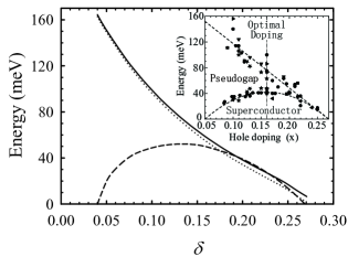
Figure 2: The bonding (2$\bar{\Delta}^{(1)}_{\rm pg}$) (dotted line) and antibonding (2$\bar{\Delta}^{(2)}_{\rm pg}$) (solid line) components of the effective normal-state pseudogap parameter, and the effective charge carrier pair gap parameter ($2\bar{\Delta}_{\rm hL}$) (dashed line) as a function of doping for temperature $T=0.002J$ with parameters $t/J=2.5$, $t^{\prime}/t=0.3$, $t_{\perp}/t=0.35$ and $J=110$ meV. Inset: the experimental data observed on different families of the cuprate superconductors taken from Ref. Hufner08, .

In Fig. 2, we plot the bonding (2$\bar{\Delta}^{(1)}_{\rm pg}$) (dotted line) and antibonding (2$\bar{\Delta}^{(2)}_{\rm pg}$) (solid line) components of the effective normal-state pseudogap parameter, and the effective charge carrier pair gap parameter ($2\bar{\Delta}_{\rm hL}$) (dashed line) as a function of doping for $T=0.002J$ with $t/J=2.5$, $t^{\prime}/t=0.3$, $t_{\perp}/t=0.35$ and $J=110$ meV in comparison with the corresponding experimental data Hufner08 observed on different families of the cuprate superconductors (inset). Obviously, both $\bar{\Delta}^{(1)}_{\rm pg}$ and $\bar{\Delta}^{(2)}_{\rm pg}$ have almost the same magnitude in a given doping concentration, which implies the transverse part of the effective normal-state pseudogap parameter $\bar{\Delta}_{\rm pgT}\approx 0$ and $\bar{\Delta}^{(1)}_{\rm pg}\approx\bar{\Delta}^{(2)}_{\rm pg}\approx\bar{\Delta}_{\rm pgL}$, then the two-gap feature observed on the bilayer cuprate superconductors Hufner08 is qualitatively reproduced. Moreover, the effective normal-state pseudogap parameter $\bar{\Delta}_{\rm pgL}$ is much larger than the effective charge carrier pair gap parameter $\bar{\Delta}_{\rm hL}$ in the underdoped regime, then it smoothly decreases with increasing the doping concentration. In particular, both $\bar{\Delta}_{\rm pgL}$ and $\bar{\Delta}_{\rm hL}$ converge to the end of the SC dome. The present result also shows that the weak charge carrier interaction directly from the interlayer coherent hopping (2) in the kinetic energy by exchanging spin excitations does not provide the contribution to the effective normal-state pseudogap in the particle-hole channel, and then the transverse part of the effective normal-state pseudogap parameter $\bar{\Delta}_{\rm pgT}\approx 0$. On the other hand, the strong charge carrier interaction directly from the intralayer hopping in the kinetic energy by exchanging spin excitations therefore can induce the normal-state pseudogap in the particle-hole channel, and then the normal-state pseudogap is dominated by the corresponding longitudinal part, i.e., $\bar{\Delta}^{(1)}_{\rm pg}\approx\bar{\Delta}^{(2)}_{\rm pg}\approx\bar{\Delta}_{\rm pgL}$, which is also consistent with the experimental results of the bilayer cuprate superconductors Hufner08 , since only one normal-state pseudogap is observed in the bilayer cuprate superconductors by using different measurement techniques Hufner08 . In combination with the previous result of the single layer case feng12 , our present study suggests that the single-layer model is sufficient for capturing the two-gap feature in cuprate superconductors.

It is well known that the many-body correlation and the related quasiparticle coherence in solids are closely related to the electron self-energy. In particular, the positions of the low-energy quasiparticle peaks in the low-energy excitation spectrum are determined by the electron self-energy. However, in the previous discussions of the electronic structure based on the kinetic energy driven SC mechanism for both the single layer and bilayer cuprate superconductors guo07 ; lan07 ; feng08 , the treatment of the charge carrier self-energy in the particle-hole channel is oversimplified, i.e., in the static limit approximation, the charge carrier self-energy in the particle-hole channel is replaced by the charge carrier coherent weight, then some subtle many-body effects from the normal-state pseudogap is abandoned, which leads to that the peak-dip-hump structure in the low-energy excitation spectrum is absent from the single layer cuprate superconductors guo07 , while the peak-dip-hump structure in the bilayer case is mainly induced by BS lan07 . Recently, the electronic structure of the single layer cuprate superconductors has been reexamined based on the kinetic energy driven SC mechanism by considering the normal-state pseudogap effect (then the many-body correlation) beyond the previous static limit approximation for the charge carrier self-energy in the particle-hole channel, and the result shows zhao12 that even in the single layer cuprate superconductors, there is an obvious peak-dip-hump structure due to the presence of the normal-state pseudogap, in qualitative agreement with the numerical result Ferrero09 based on the dynamical MF theory. In combination this result zhao12 for the single layer cuprate superconductors and the previous result lan07 for the bilayer case, it suggests that both the normal-state pseudogap and BS induce the peak-dip-hump structure in the bilayer cuprate superconductors, however, the notable peak-dip-hump structure in the bilayer cuprate superconductors may be mainly dominated by BS.

The essential physics of the two-gap feature in the bilayer cuprate superconductors is the same as in the single layer case feng12 , and can be attributed to the doping and temperature dependence of the charge carrier interactions in the particle-hole and particle-particle channels directly from the kinetic energy by exchanging spin excitations. Our present results also indicate that although BS due to the presence of the interlayer coherent hopping (2) can play an important role in the form of the peak-dip-hump structure around the antinodal point lan07 ; feng08 , it may have not an impact on the overall global feature for the SC gap and normal-state pseudogap parameters. This follows a fact that BS is maximum around the antinodal point, and it vanishes along the nodal direction. As an result, this momentum dependence of BS has an impact on the momentum dependence of the peak-dip-hump structure, while it does no has an effect on the momentum independence of the SC gap and normal-state pseudogap parameters. Furthermore, in the present bilayer case, we have also calculated the doping dependence of the coupling strength $V_{\rm eff}$, and the result shows that as in the single layer case feng12 , the coupling strength $V_{\rm eff}$ smoothly decreases upon increasing the doping concentration from a strong-coupling case in the underdoped regime to a weak-coupling side in the overdoped regime. Since the charge carrier interactions in both the particle-hole and particle-particle channels are mediated by the same spin excitations as shown in Eq. (8), therefore all these charge carrier interactions are controlled by the same magnetic interaction $J$. In this sense, both the normal-state pseudogap and SC gap in the phase diagram of the bilayer cuprate superconductors are dominated by one energy scale. This is why both $\bar{\Delta}_{\rm pgT}\approx 0$ (then $\bar{\Delta}^{(1)}_{\rm pg}\approx\bar{\Delta}^{(2)}_{\rm pg}\approx\bar{\Delta}_{\rm pgL}$) and $\bar{\Delta}_{\rm hT}\approx 0$ (then $\bar{\Delta}^{(1)}_{\rm h}\approx\bar{\Delta}^{(2)}_{\rm h}\approx\bar{\Delta}_{\rm hL}$) simultaneously in the bilayer cuprate superconductors, and then the two-gap behavior is a universal feature for the single layer and bilayer cuprate superconductors.

In conclusion, we have discussed the interplay between the SC gap and normal-state pseudogap in the bilayer cuprate superconductors based on the framework of the kinetic energy driven SC mechanism. Our results show that the single-layer model is sufficient for capturing the two-gap feature in cuprate superconductors. The weak charge carrier interaction directly from the interlayer coherent hopping (2) in the kinetic energy by exchanging spin excitations does not provide the contribution to the normal-state pseudogap in the particle-hole channel and charge carrier pair gap in the particle-particle channel, which leads to that the transverse parts of the effective normal-state pseudogap parameter $\bar{\Delta}_{\rm pgT}\approx 0$ and effective charge carrier pair gap parameter $\bar{\Delta}_{\rm hT}\approx 0$ simultaneously, while only the strong charge carrier interaction directly from the intralayer hopping in the kinetic energy by exchanging spin excitations therefore induces the normal-state pseudogap in the particle-hole channel and charge carrier pair gap in the particle-particle channel, and then the normal-state pseudogap and charge carrier pair gap are dominated by the corresponding longitudinal parts, i.e., $\bar{\Delta}^{(1)}_{\rm pg}\approx\bar{\Delta}^{(2)}_{\rm pg}\approx\bar{\Delta}_{\rm pgL}$ and $\bar{\Delta}^{(1)}_{\rm h}\approx\bar{\Delta}^{(2)}_{\rm h}\approx\bar{\Delta}_{\rm hL}$.

References

• (1) J. R. Schrieffer, Theory of Superconductivity (Addison-Wesley, San Francisco, 1964).
• (2) See, e.g., S. Hüfner, M. A. Hossain, A. Damascelli, and G. A. Sawatzky, Rep. Prog. Phys. 71, 062501 (2008), and references therein.
• (3) See, e.g., Tom Timusk and Bryan Statt, Rep. Prog. Phys. 62, 61 (1999), and references therein.
• (4) See, e.g., A. Damascelli, Z. Hussain, and Z.-X. Shen, Rev. Mod. Phys. 75, 473 (2003), and references therein.
• (5) See, e.g., J. C. Campuzano, M. R. Norman, and M. Randeira, in Physics of Superconductors, vol. II, edited by K. Bennemann and J. Ketterson (Springer, Berlin Heidelberg New York, 2004), p. 167, and references therein.
• (6) J. C. Campuzano, H. Ding, M. R. Norman, M. Randeira, A. F. Bellman, T. Yokoya, T. Takahashi, H. Katayama-Yoshida, T. Mochiku, and K. Kadowaki, Phys. Rev. B 53, R14737 (1996); H. Matsui, T. Sato, T. Takahashi, S.-C. Wang, H.-B. Yang, H. Ding, T. Fujii, T. Watanabe, and A. Matsuda, Phys. Rev. Lett. 90, 217002 (2003).
• (7) D. L. Feng, N. P. Armitage, D. H. Lu, A. Damascelli, J. P. Hu, P. Bogdanov, A. Lanzara, F. Ronning, K. M. Shen, H. Eisaki, C. Kim, Z.-X. Shen, J.-i. Shimoyama, and K. Kishio, Phys. Rev. Lett. 86, 5550 (2001); A. A. Kordyuk, S. V. Borisenko, M. Knupfer, and J. Fink, Phys. Rev. B 67, 064504 (2003); Y.-D. Chuang, A. D. Gromko, A. Fedorov, Y. Aiura, K. Oka, Y. Ando, H. Eisaki, S. I. Uchida, and D. S. Dessau, Phys. Rev. Lett. 87, 117002 (2001).
• (8) Yu Lan, Jihong Qin, and Shiping Feng, Phys. Rev. B 75, 134513 (2007); Yu Lan, Jihong Qin, and Shiping Feng, Phys. Rev. B 76, 014533 (2007).
• (9) A. A. Kordyuk, S. V. Borisenko, T. K. Kim, K. A. Nenkov, M. Knupfer, J. Fink, M. S. Golden, H. Berger, and R. Follath, Phys. Rev. Lett. 89, 077003 (2002).
• (10) S. V. Borisenko, A. A. Kordyuk, T. K. Kim, A. Koitzsch, M. Knupfer, J. Fink, M. S. Golden, M. Eschrig, H. Berger, and R. Follath, Phys. Rev. Lett. 90, 207001 (2003); S. V. Borisenko, A. A. Kordyuk, T. K. Kim, S. Legner, K. A. Nenkov, M. Knupfer, M.S. Golden, J. Fink, H. Berger, and R. Follath, Phys. Rev. B 66, 140509 (2002).
• (11) Shiping Feng, Phys. Rev. B 68, 184501 (2003); Shiping Feng, Tianxing Ma, and Huaiming Guo, Physica C 436, 14 (2006).
• (12) Shiping Feng, Huaisong Zhao, and Zheyu Huang, Phys. Rev. B 85, 054509 (2012).
• (13) P. W. Anderson, Science 235, 1196 (1987).
• (14) O. K. Anderson, A. I. Liechtenstein, O. Jepsen, and F. Paulsen, J. Phys. Chem. Solids 56, 1573 (1995); A. I. Liechtenstein, O. Gunnarsson, O. K. Anderson, and R. M. Martin, Phys. Rev. B 54, 12505 (1996).
• (15) Shiping Feng, Jihong Qin, and Tianxing Ma, J. Phys.: Condens. Matter 16, 343 (2004).
• (16) See, e.g., the review, Shiping Feng, Huaiming Guo, Yu Lan, and Li Cheng, Int. J. Mod. Phys. B 22, 3757 (2008).
• (17) G. M. Eliashberg, Sov. Phys. JETP 11, 696 (1960); D. J. Scalapino, J. R. Schrieffer, and J. W. Wilkins, Phys. Rev. 148, 263 (1966).
• (18) Huaiming Guo and Shiping Feng, Phys. Lett. A 361, 382 (2007).
• (19) Huaisong Zhao, Lülin Kuang, and Shiping Feng, Physica C 483, 225 (2012); Huaisong Zhao and Shiping Feng, unpublished.
• (20) Michel Ferrero, Pablo S. Cornaglia, Lorenzo De Leo, Olivier Parcollet, Gabriel Kotliar, and Antoine Georges, Phys. Rev. B 80, 064501 (2009).