PHYSICAL PROPERTIES OF SPECTROSCOPICALLY-CONFIRMED GALAXIES AT $z\geq 6$. I. BASIC CHARACTERISTICS OF THE REST-FRAME UV CONTINUUM AND LYMAN-$\alpha$ EMISSION

Abstract

We present deep HST near-IR and Spitzer mid-IR observations of a large sample of spectroscopically-confirmed galaxies at $z\geq 6$. The sample consists of 51 Ly$\alpha$ emitters (LAEs) at $z\simeq 5.7$, 6.5, and 7.0, and 16 Lyman-break galaxies (LBGs) at $5.9\leq z\leq 6.5$. The near-IR images were mostly obtained with WFC3 in the F125W and F160W bands, and the mid-IR images were obtained with IRAC in the $3.6\mu$m and $4.5\mu$m bands. Our galaxies also have deep optical imaging data from Subaru Suprime-Cam. We utilize the multi-band data and secure redshifts to derive their rest-frame UV properties. These galaxies have steep UV continuum slopes roughly between $\beta\simeq-1.5$ and –3.5, with an average value of $\beta\simeq-2.3$, slightly steeper than the slopes of LBGs in previous studies. The slope shows little dependence on UV continuum luminosity except for a few of the brightest galaxies. We find a statistically significant excess of galaxies with slopes around $\beta\simeq-3$, suggesting the existence of very young stellar populations with extremely low metallicity and dust content. Our galaxies have moderately strong rest-frame Ly$\alpha$ equivalent width (EW) in a range of $\sim$10 to $\sim$200 Å. The star-formation rates are also moderate, from a few to a few tens solar masses per year. The LAEs and LBGs in this sample share many common properties, implying that LAEs represent a subset of LBGs with strong Ly$\alpha$ emission. Finally, the comparison of the UV luminosity functions between LAEs and LBGs suggests that there exists a substantial population of faint galaxies with weak Ly$\alpha$ emission ($\rm EW<20$ Å) that could be the dominant contribution to the total ionizing flux at $z\geq 6$.

1. INTRODUCTION

The epoch of cosmic reionization marks one of the major phase transitions of the Universe, during which the neutral intergalactic medium (IGM) was ionized by the first astrophysical objects. Measurements of CMB polarization have shown that reionization began earlier than $z\simeq 10.6$ (Komatsu et al., 2011). Meanwhile, studies of Gunn-Peterson troughs in high-redshift quasar spectra have located the end of reionization at $z\simeq 6$ (Fan et al., 2006). Therefore, objects at $z\geq 6$ are natural tools to probe this epoch. With recent advances of instrumentation on Hubble Space Telescope ($HST$) and large ground-based telescopes, galaxies at $z\geq 6$ are now being routinely found. Direct observations of the earliest galaxy formation and the history of reionization are finally in sight (Robertson et al., 2010; Finlator, 2012).

The first $z>6$ galaxies were discovered to be Ly$\alpha$ emitters (LAEs) at $z\simeq 6.5$ using the narrow-band (or Ly$\alpha$) technique (Hu et al., 2002; Kodaira et al., 2003; Rhoads et al., 2004). This technique has been an efficient way to find high-redshift galaxies due to its high success rate of spectroscopic confirmation. Three dark atmospheric windows with little OH sky emission in the optical are often used to detect distant galaxies at $z\simeq 5.7$, 6.5, and 7. So far more than 200 LAEs have been spectroscopically confirmed at these redshifts (e.g., Taniguchi et al., 2005; Iye et al., 2006; Shimasaku et al., 2006; Kashikawa et al., 2006, 2011; Hu et al., 2010; Ouchi et al., 2010; Rhoads et al., 2012). The narrow-band technique is also being used to search for higher redshift LAEs at $z>7$ (e.g., Hibon et al., 2010; Tilvi et al., 2010; Clément et al., 2012; Krug et al., 2012; Ota & Iye, 2012; Shibuya et al., 2012). All these Ly$\alpha$ surveys were made with ground-based instruments owing to their large field-of-views (FOVs) and relatively low sky-background in OH-dark windows.

A complementary way to find high-redshift galaxies is the dropout technique (Steidel & Hamilton, 1993; Giavalisco, 2002). It has produced a large number of Lyman-break galaxies (LBGs) or candidates at $z\geq 6$. While large-area ground-based observations are efficient to select bright LBGs (e.g., Nagao et al., 2007; Bowler et al., 2012; Curtis-Lake et al., 2012; Hsieh et al., 2012; Willott et al., 2013), the majority of the faint LBGs at $z\geq 6$ known so far were discovered by $HST$ (e.g., Bunker et al., 2004; Dickinson et al., 2004; Yan & Windhorst, 2004). In particular, with the power of the new $HST$ WFC3 infrared camera, a few hundred galaxies at $6\leq z\leq 12$ have been detected recently (e.g., Bunker et al., 2010; Finkelstein et al., 2010; McLure et al., 2010; Oesch et al., 2010; Wilkins et al., 2010; Yan et al., 2010; Bouwens et al., 2011; Lorenzoni et al., 2011; Ellis et al., 2013). Although most of the LBG candidates are too faint for follow-up identification, some of them have been spectroscopically confirmed with deep ground-based observations (e.g., Stark et al., 2010, 2011; Jiang et al., 2011; Vanzella et al., 2011; Pentericci et al., 2011; Ono et al., 2012; Schenker et al., 2012).

With the large samples of galaxies (and candidates) at $z\geq 6$, the UV continuum luminosity function (LF) and Ly$\alpha$ LF are being established (e.g., Hu et al., 2010; Jiang et al., 2011; Kashikawa et al., 2011; Bradley et al., 2012; Bouwens et al., 2012a; Henry et al., 2012; Laporte et al., 2012; Oesch et al., 2012). It is found that the faint-end slope of the UV LFs are very steep ($\alpha\simeq-2$), so dwarf galaxies could provide enough UV photons for reionization (also depending on the ionizing photon escape fraction and the ionized gas clumping factor). For individual galaxies, their physical properties are also being investigated. At $z\geq 6$, the rest-frame UV/optical light moves to the infrared range. Therefore, infrared observations, especially the combination of $HST$ and Spitzer Space Telescope ($Spitzer$), are essential to measure properties of these high-redshift galaxies. $HST$ near-IR data constrain the slope of the rest-frame UV spectrum and help to decipher the properties of young stellar populations. Recent $HST$ WFC3 near-IR observations have shown that high-redshift LBGs have blue rest-frame UV slopes $\beta$ ($f_{\lambda}\propto{\lambda}^{\beta}$). The typical values of $\beta$ are close to or smaller (bluer) than –2 (e.g., Wilkins et al., 2011; Bouwens et al., 2012b; Dunlop et al., 2012a; Finkelstein et al., 2012). Though the selection criteria of LBGs and the approaches to UV slopes are slightly different in the different studies in the literature, it is believed that $z\geq 6$ galaxies are bluer than low-redshift galaxies, implying that they are generally younger and have low dust extinction.

More detailed physical properties (e.g. age and stellar mass) of high-redshift galaxies have come from SED modeling based on broad-band photometry of $HST$ and $Spitzer$ as well as optical data. $Spitzer$ IRAC provides mid-IR photometry. When combined with $HST$ near-IR data, it measures the amplitude of the Balmer break and constrains the properties of mature populations. The early results on $z\simeq 6$ LBGs showed IRAC detections, and emphasized galaxies with established stellar populations (e.g., Egami et al., 2005; Eyles et al., 2005; Yan et al., 2005). Later studies found that most LBGs were actually not detected in moderately deep IRAC images, suggesting that these galaxies were considerably younger and less massive (e.g., Yan et al., 2006; Eyles et al., 2007). LAEs may represent an even more extreme population with ages of only a few million years (e.g., Pirzkal et al., 2007). As the number of galaxies known at $z\geq 6$ increases steadily, extensive studies are being carried out on various galaxy samples (e.g., González et al., 2010; Ono et al., 2010; Schaerer & de Barros, 2010; McLure et al., 2011; Pirzkal et al., 2012). A diversity of physical properties are found among these galaxies, although the Universe is younger than one billion years.

Despite the progress that has been made on properties of high-redshift galaxies, there is a lack of a large, reliable sample of $z\geq 6$ galaxies with spectroscopic redshifts and high-quality infrared photometry. The reason is twofold. For galaxies found by ground-based telescopes — although they are relatively bright and have spectroscopic redshifts — they often do not have measured infrared (rest-frame UV/optical) information. For example, only a small amount of LAEs at $z\geq 6$ have been observed in the near-IR bands by $HST$ (e.g., Cowie et al., 2011a). On the other hand, galaxies found by $HST$ (e.g. those in the GOODS fields), do have near-IR photometry, but most of them are too faint for follow-up spectroscopic identification by current facilities. So they do not have secure redshifts, making it difficult for accurate SED modeling. A model SED derived from a few photometric points without a secure redshift is usually highly degenerate. Therefore, determination of the physical properties of $z\geq 6$ galaxies demands a large sample of galaxies with both spectroscopic redshifts and high-quality infrared photometry.

In this paper we will present deep $HST$ and $Spitzer$ observations of 67 spectroscopically-confirmed (hereafter spec-confirmed) galaxies at $z\geq 6$. This galaxy sample contains 51 LAEs and 16 LBGs, and is the largest collection of spec-confirmed galaxies in this redshift range. The spectroscopic redshifts of the sample provide great advantages for measuring the physical properties of galaxies. First, this sample is uncontaminated by interlopers. A photometrically-selected (hereafter photo-selected) sample of high-redshift galaxies may be contaminated by interlopers such as low-redshift red or dusty galaxies and Galactic late-type dwarf stars, which may cause various bias on measurements of physical properties. Second, spectroscopic redshifts remove one critical free parameter for SED modeling. For the brightest galaxies at $z\geq 6$, there are usually only 4–5 broad-band photometric points available (e.g., two $HST$ bands, two $Spitzer$ IRAC bands, and one optical band) for producing stellar population models. Given the limited degrees of freedom, a spectroscopic redshift will significantly improve SED modeling, especially when nebular emission is considered. At $z\geq 6$, strong nebular emission lines such as [O iii] $\lambda$5007, H$\beta$, and H$\alpha$ enter IRAC 1 and 2 channels, which affect our estimate of stellar populations (e.g., Schaerer & de Barros, 2010; Finlator et al., 2011; de Barros et al., 2012; Stark et al., 2013). Photometric redshifts with large uncertainties may place these nebular lines in wrong bands during SED fitting. With spectroscopic redshifts, the positions of nebular lines are secured (see Stark et al. 2012 for more discussion). Finally, we currently have little knowledge of stellar populations in $z\geq 5.5$ LAEs. This is because almost all the known LAEs were discovered by ground-based telescopes, and most of them do not have infrared observations. Our paper includes a large sample of LAEs. This allows us, for the first time, to systematically study stellar populations in LAEs.

This paper is the first in a series presenting the physical properties of these galaxies based on observations from $HST$, $Spitzer$, and the Subaru telescope. The vast majority of the galaxies were discovered in the Subaru Deep Field (SDF; Kashikawa et al., 2004). The SDF is a unique and ideal field to study the distant Universe: it covers an area of over 800 arcmin² and has the deepest optical images among all ground-based imaging data. The SDF project has been highly successful in searching for high-redshift galaxies. It has identified more than 100 LAEs and LBGs at $z\geq 6$ (e.g., Taniguchi et al., 2005; Iye et al., 2006; Shimasaku et al., 2006; Nagao et al., 2007; Ota et al., 2008; Jiang et al., 2011; Kashikawa et al., 2011; Toshikawa et al., 2012). These galaxies are spectroscopically confirmed and represent the most luminous galaxies in this redshift range. In this paper we present the $HST$ and $Spitzer$ observations, and use these data together with the optical data from Subaru to derive the rest-frame UV properties, such as their UV continuum slopes $\beta$ and Ly$\alpha$ luminosities. In the subsequent papers of this series we will present rest-frame UV morphology and measure stellar populations for these galaxies.

The structure of the paper is as follows. In Section 2, we present our galaxy sample. We also describe our optical/infrared observations and data reduction. In Section 3, we derive the rest-frame UV continuum properties of the galaxies. In Section 4, we measure the properties of Ly$\alpha$ emission lines. We discuss our results in Section 5 and summarize the paper in Section 6. Throughout the paper we use a $\Lambda$-dominated flat cosmology with $H_{0}=70$ km s^-1 Mpc^-1, $\Omega_{m}=0.3$, and $\Omega_{\Lambda}=0.7$ (Komatsu et al., 2011). All magnitudes are on the AB system (Oke & Gunn, 1983).

2. OBSERVATIONS AND DATA REDUCTION

2.1. Galaxy Sample

Table 1 shows the list of the galaxies presented in this paper. There are a total of 67 spec-confirmed galaxies at $5.6\leq z\leq 7$: 62 of them are from the SDF and the remaining 5 are from the Subaru XMM-Newton Deep Survey (SXDS; Furusawa et al., 2008) field. They represent the most luminous galaxies in terms of Ly$\alpha$ luminosity for LAEs or UV continuum luminosity for LBGs in this redshift range.

The SDF covers an area of $\sim 876$ arcmin², and its optical imaging data were taken with Subaru Suprime-Cam in a series of broad and narrow bands (Kashikawa et al., 2004). Especially noteworthy are the deep observations with three narrow-band (NB) filters, NB816, NB921, and NB973, corresponding to the detection of LAEs at $z\simeq 5.7$, 6.5, and 7. The full widths at half maximum (FWHM) of the three filters are 120, 132, and 200 Å, respectively. So far the SDF project has spectroscopically confirmed more than 100 LAEs at $z\simeq 5.7$, 6.5, 7, and more than 40 LBGs at $6\leq z\leq 7$. Our SDF galaxy sample contains 22 LAEs at $z\simeq 5.7$ (Shimasaku et al., 2006; Kashikawa et al., 2011), 25 LAEs at $z\simeq 6.5$ (Taniguchi et al., 2005; Kashikawa et al., 2006, 2011), and the $z=6.96$ LAE (Iye et al., 2006). The LAEs at $z\simeq 5.7$ and 6.5 were selected in a similar way, and have a relatively uniform magnitude limit of 26 mag in the narrow bands NB816 and NB921, so they are from a well-defined flux-limited sample. Our SDF sample also contains 14 LBGs at $5.9\leq z\leq 6.5$ (Nagao et al., 2004, 2005, 2007; Ota et al., 2008; Jiang et al., 2011); two of them have not been previously published. These LBGs were selected with different criteria and thus have inhomogeneous depth. The $z^{\prime}$-band magnitude limit is 26.1 mag in Nagao et al. papers, 26.5 mag in Ota et al. (2008), and 27 mag in Jiang et al. (2011). For the details of candidate selection and follow-up spectroscopy, see the original galaxy discovery papers above.

Five galaxies in our sample, including 2 LBGs at $z\simeq 6$ (Curtis-Lake et al., 2012) and 3 LAEs at $z\simeq 6.5$ (Ouchi et al., 2010), are from the SXDS. The two LBGs are very bright ($z^{\prime}<25$ mag) and have been analyzed by Curtis-Lake et al. (2013). The SXDS optical imaging data were also taken with Subaru Suprime-Cam in the same broad and narrow bands, but cover five times larger area than the SDF does (Furusawa et al., 2008).

In Table 1, the first 62 galaxies are from the SDF and the last 5 galaxies are from the SXDS. Columns 2 and 3 list the object coordinates. They are re-calculated from our own stacked optical images (see Section 2.2), and are fully consistent with those given in the galaxy discovery papers (typical difference $<0\farcs 1$). Column 4 lists the redshifts, measured from the Ly$\alpha$ emission lines of the galaxies. The galaxy discovery papers used different values for the rest-frame Ly$\alpha$ wavelengths (i.e. 1215, 1215.67, or 1216 Å) for redshift measurements. We convert all these redshifts to the redshifts listed in Table 1 by assuming a rest-frame Ly$\alpha$ line center of 1215.67 Å. The last column shows the reference papers of the objects. We will explain the rest of the table in the following subsections.

2.2. Optical Imaging Data

The galaxies in this paper were discovered in the SDF and the SXDS. The SDF public imaging data include stacked images in five broad bands $BVRi^{\prime}z^{\prime}$ and two narrow bands NB816 and NB921. The flux limits for these data are given in Kashikawa et al. (2004). However, the public data do not include the data taken recently (also by Subaru Suprime-Cam), and the data taken in the $y$ and NB973 bands. Therefore, we produced our own stacked images by including all available images in the Subaru archive, as explained below.

Our data processing began with the raw images obtained from the archival server SMOKA (Baba et al., 2002). Raw images with point spread function (PSF) sizes greater than $1\farcs 2$ were rejected. The data were reduced, re-sampled, and co-added using a combination of the Suprime-Cam Deep Field REDuction package (SDFRED; Yagi et al., 2002; Ouchi et al., 2004) and our own IDL routines. Each image was bias (overscan) corrected and flat-fielded using SDFRED. Then bad pixel masks were created from flat-field images. Cosmic rays were identified and interpolated using L.A. Cosmic (van Dokkum, 2001). Saturated pixels and bleeding trails were also identified and interpolated. For each image, a weight mask was generated to include all above mentioned defective pixels. We then used SDFRED to correct the image distortion, subtract the sky-background, and mask out the pixels affected by the Auto-Guider probe. After individual images were processed, we extracted sources using SExtractor (Bertin & Arnouts, 1996) and calculated astrometric and photometric solutions using SCAMP (Bertin, 2006) for the final image co-addition. In order to match the public SDF images, we used the public $R$-band image as the astrometric reference catalog in SCAMP. Both science and weight-map images were scaled and updated using the astrometric and photometric solutions measured from SCAMP. Instead of homogenizing PSFs to a certain value as was done for the public data, we incorporated PSF information into the weight image so that the weight was proportional to the inverse of the square of the PSF FWHM. We re-sampled and co-added images using SWARP (Bertin et al., 2002). The re-sampling interpolations for science and weight images were LANCZOS3 and BILINEAR, respectively. We modified SWARP so that it performs sigma-clipping ($5\sigma$ rejection) of outliers when co-adding images.

We produced images in the six broad bands $BVRi^{\prime}z^{\prime}y$ and three narrow bands NB816, NB921, and NB973. The final products are a stacked science image, and its corresponding weight image, for each band. The pixel and image sizes of our products are the same as those of the public SDF images. The typical PSF FWHM is $0\farcs 6-0\farcs 7$. We determined photometric zero points from the public SDF images whose zero points were known. The SXDS optical imaging data were reduced in the same way as we did for the SDF.

Our SDF broad-band images are deeper than the public images in the $Ri^{\prime}z^{\prime}$ bands, because the SDF team obtained more imaging data from Subaru recently, and we included all the available data above. For example, the public $z^{\prime}$-band image has a depth of $z^{\prime}=26.1$ mag ($5\sigma$ detection in a $2\arcsec$ diameter aperture) with a total integration time of $\sim$7 hr. To date, the total $z^{\prime}$-band data amount to $\sim$29 hr. Our new $z^{\prime}$-band image has a depth of $\sim$27.0 mag, 0.9 mag deeper than the public image. In addition, the public data do not have images in the $y$ and NB973 bands. The SDF $y$-band imaging data were taken with two different sets of CCDs (MIT and Hamamatsu), and have been used to search for $z\simeq 7$ LBGs (Ouchi et al., 2009). Although the fully-depleted Hamamatsu CCDs are twice as sensitive as the MIT CCDs in the $y$ band, their sensitivity (quantum efficiency) curves have similar shapes. Therefore, we stacked all the images taken with both sets of CCDs, as Ouchi et al. (2009) did in their work. The total integration time was 24 hr, and the depth was about 26.0 mag.

In Table 1, Columns 5 to 7 show the total magnitudes of the galaxies in one of the three narrow bands (NB816, NB921, or NB973, depending on redshift) and two broad bands $z^{\prime}y$. For a given object in a given filter, its total magnitude is measured as follows. We first use SExtractor to measure the aperture photometry of the object in a circular $2\farcs 0$ diameter, after the local sky-background is subtracted. In cases where galaxies are close to their neighbors, we use a circular $1\farcs 6$ diameter. Then an aperture correction is applied to correct for light loss. The aperture correction is determined from more than 100 bright, but unsaturated point sources in the same image. Almost all our galaxies are point-like objects and are not resolved in the SDF images. In cases where galaxies clearly show extended features, we use MAG_AUTO magnitudes as the best estimates of the total magnitudes. In Table 1, we did not list broad-band photometry for the galaxies with weak detections ($<5\sigma$) in the $J$ band. These galaxies are excluded in most of our analysis in this paper. Detections below $3\sigma$ in any of these bands are not listed as well. We carefully check each object, and find that object no. 12, a $z\simeq 5.7$ LAE, is overlapped by a bright foreground star (this was also pointed out in the galaxy discovery paper). The separation between the two objects is only $\sim 0\farcs 25$, so we are not able to do photometry for this galaxy. We will not use this galaxy in the following analysis.

Figure 1 shows the transmission curves of six Subaru Suprime-Cam filters, including three broad-band filters $i^{\prime}z^{\prime}y$ and three narrow-band filters NB816, NB921, and NB973. We do not show the other three bluer filters $BVR$, because our galaxies were not detected in these bands. In Appendix A, we show the thumbnail images of the galaxies in one of the three Subaru Suprime-Cam narrow bands and the three broad bands $i$, $z^{\prime}$, and $y$.

2.3. $HST$ Near-IR Imaging Data

We obtained $HST$ near-IR imaging data for a large sample of spectroscopically confirmed SDF galaxies at $5.6\leq z\leq 7$ from three $HST$ GO programs 11149 (PI: E. Egami), 12329 and 12616 (PI: L. Jiang). The three programs together with our $Spitzer$ programs (see the next subsection) were designed to characterize the physical properties of these high-redshift galaxies. The $HST$ observations were made with a mix of strategies. As the proposal for GO program 11149 was written, $HST$ WFC3 had not yet been installed. Our plan was to observe 20 bright galaxies with NICMOS in the F110W (hereafter $J_{110}$) and F160W (hereafter $H_{160}$) bands. The observations were made with camera NIC3. The exposure time was two orbits per band per pointing (or per object), split into four exposures. The total on-source integration per band was about 5400 sec. We performed sub-pixel dithering during the four NICMOS exposures to improve the PSF sampling and to remove bad pixels and cosmic rays.

After we finished several targets, NICMOS failed, and then WFC3 was installed in May 2009. Since WFC3 has much higher sensitivity, the rest of the galaxies in GO 11149 and all the galaxies in GO 12329 and 12616 were observed with WFC3. Because of the larger FOV of WFC3 and the increasing number of known $z\geq 6$ galaxies in the SDF, we changed our observing strategy for GO 12329 and 12616. We chose the regions that cover at least 3 galaxies (up to 5) per $HST$/WFC3 pointing. By doing this we were able to observe many galaxies in a small number of telescope pointings. We used F125W (hereafter $J_{125}$) and $H_{160}$ in these two programs. In GO 12329, the exposure time was one orbit per filter per pointing. We found that some galaxies in our sample were barely detected with this depth. Therefore in GO 12616, all new WFC3 pointings had a depth of two orbits (on-source integration $\sim 4800$ sec; see Windhorst et al. 2011 for the anticipated sensitivity in two-orbit WFC3 exposures). We also re-observed most galaxies that were observed in GO 12329, so that they have a total of two-orbit depth per band. As in the NICMOS observations above, the WFC3 observation of each pointing (per band) was split into four exposures. Sub-pixel dithering during the exposures was also performed to improve the PSF sampling and to remove bad pixels and cosmic rays. The transmission curves of the three WFC3 filters are plotted in Figure 1.

As we mentioned above, several galaxies in our sample were found in the SXDS. They were covered by the UKIDSS Ultra-Deep Survey (UDS). Their $HST$ WFC3 near-IR data were obtained from the Cosmic Assembly Near-infrared Deep Extragalactic Legacy Survey (CANDELS; Grogin et al., 2011; Koekemoer et al., 2011). The exposure depth of the CANDELS UDS data is 1900 sec in the $J_{125}$ band and 3300 sec in the $H_{160}$ band. They are shallower than our WFC3 data for the SDF.

In Appendix A we show the thumbnail images of the galaxies in the two $HST$ near-IR bands $J_{110}$ (or $J_{125}$) and $H_{160}$. Note that the $J_{125}$-band image of the $z=6.96$ LAE (no. 62) was obtained from GO program 11587 (Cai et al., 2011). This image also covers another two objects (no. 2 and no. 59) in our sample. Due to the high sensitivity of WFC3, the majority of the galaxies in our sample are detected with high significance in the near-IR images. Only 15 of them — among the faintest in the optical bands — have weak detections ($<5\sigma$) in the $J$ band.

Our WFC3 data processing began with individual flat-fielded, flux calibrated WFC3 infrared exposures delivered by the $HST$ archive. Each pointing used a standard 4-point dither pattern to obtain uniform half-pixel sampling. All exposures for each pointing were combined using the software Multidrizzle (Koekemoer et al., 2002), with an output plate scale of $0\farcs 06$ per pixel and a pixfrac parameter of 0.8. For our observations, this provides Nyquist sampling of the PSF and relatively uniform weighting of individual pixels. RMS maps were also derived from the Multidrizzle weight-map images, following the procedure used in Dickinson et al. (2004) that accounts for correlated noise in the final images.

Our NICMOS NIC3 data were reduced using a fully automated pipeline NICRED (Magee et al., 2007). NICRED starts its processing with raw science data and calibration files, and sequentially runs a set of steps from basic calibration to final mosaic generation. The most important part of the reduction is the basic calibration, because the NICMOS data suffer from variable bias, electronic ghosts, and cosmic-ray persistence. The basic procedure is as follows. NICRED first removes electronic ghosts, handles variable bias, rejects cosmic rays, and subtracts sky background. It then removes possible cosmic-ray persistence and residual instrument signatures. The rest of the procedure are common steps, including flat fielding, a non-linearity correction, image alignment and registration, etc. It finally creates drizzled images and the corresponding weight maps. The pixel size in the final products is $0\farcs 1$, a half of the native size.

We list the near-IR photometry of the galaxies in Columns 8 to 10 in Table 1. All galaxies were observed in the $H_{160}$ band and one or two of the $J$ bands ($J_{110}$ and/or $J_{125}$). We perform photometry using SExtractor in dual-image mode with RMS map weighting. The $J$-band is used as the detection image. A single set of parameters is used for detection in all images. We compute the total magnitudes of the objects in both filters by using MAG_AUTO elliptical apertures, with a Kron factor of 1.8 and a minimum aperture of 2.5 semi-major radius, then applying aperture corrections. The aperture corrections are calculated by running SExtractor again with five Kron factors between 2.0 and 4.0, analyzing thousands of sources in the range $J<26$ mag. We calculate a sequence of median correction vs. Kron factor, which we extend to infinite radius with an exponential fit. All final photometry apertures are visually inspected, to screen against contamination from nearby objects or spurious detections. Detections below $5\sigma$ in the $J$ band, or detections below $3\sigma$ in the $H$ band, are not listed in Table 1.

2.4. $Spitzer$ Mid-IR Imaging Data

We obtained $Spitzer$ IRAC imaging data for the SDF from two GO programs 40026 (PI: E. Egami) and 70094 (PI: L. Jiang). In GO 40026, we observed 20 luminous galaxies at $z\geq 6$, which were also the targets of our $HST$ program 11149. The observations were made in IRAC channel 1 (3.6 $\mu$m) and channel 2 (4.5 $\mu$m). The other two channels (5.8 and 8.0 $\mu$m) were observed simultaneously. We used the cycling dither pattern with medium steps and a frame exposure time of 100 sec. The on-source integration time per channel per pointing is 3 hr. In GO 70094 (during the $Spitzer$ warm mission), we modified our observing strategy and observed high galaxy surface density regions, so that we can observe a large number of galaxies with slightly more than 10 telescope pointings. The cycling dither pattern with small steps was used with a frame exposure time of 100 sec. We focused on IRAC channel 1 and increased on-source integration time to $\sim$6 hr per pointing. The two programs imaged roughly 70% of the SDF to a depth of 3–6 hours. They covered all the 62 SDF galaxies in channel 1 and 51 (out of 62) galaxies in channel 2.

The IRAC Data processing began with the cBCD (corrected BCD) products and associated mask and uncertainty images delivered by the $Spitzer$ Science Center (SSC) archive. The image fits headers were updated to match the astrometry in the SDF optical images. Then the images were processed, drizzled, and co-added using using the SSC pipeline MOPEX. This is a fully automated procedure. The final images have a pixel size of $0\farcs 6$, roughly a half of the IRAC native pixel scale. The IRAC images for the SXDS galaxies were obtained from the SSC archive (programs 60022 and 80057). The data were reduced in the same way above. In Appendix (the last two columns) we show the thumbnail images of the galaxies in the two IRAC channels.

Mid-IR photometry is complicated by source confusion. Galaxies in deep IRAC images are often blended with nearby neighbors, so accurate photometry requires proper deblending and removing neighbors. We will present IRAC photometry of our galaxies in the second paper of this series.

3. REST-FRAME UV CONTINUUM PROPERTIES

With the narrow- and broad-band photometry from the NB816 to the $H_{160}$ band, we are able to measure the spectral properties, such as Ly$\alpha$ flux and UV continuum slopes, for most of the galaxies in this sample. In order to measure the rest-frame UV properties, we produce a model spectrum for each of these galaxies. The model spectrum $f_{\rm gal}$ (in units of $\rm erg\ s^{-1}\ cm^{-2}\ A^{-1}$, like commonly used $f_{\lambda}$) is the sum of a Ly$\alpha$ emission line and a power-law UV continuum with a slope $\beta$,

$$f_{\rm gal}=A\times S_{\rm Ly\alpha}+B\times{\lambda}^{\beta},$$ (1)

where $A$ and $B$ are scaling factors in units of $\rm erg\ s^{-1}\ cm^{-2}\ A^{-1}$, and $S_{\rm Ly\alpha}$ (dimensionless) is the Ly$\alpha$ emission line profile. In the redshift range and wavelength range considered here, other nebular lines such as He ii $\lambda$1640 can be safely ignored (e.g., Cai et al., 2011). We first determine the continuum parameters $B$ and $\beta$ by fitting the continuum $f_{\rm con,\lambda}=B\times{\lambda}^{\beta}$ (or $f_{\rm con,\nu}\propto{\lambda}^{\beta+2}$) with the broad-band data that do not cover the Ly$\alpha$ emission. Because AB magnitude $m_{\rm AB}$ and $\rm Log(\lambda)$ have the simplest linear relation $m_{\rm AB}\propto(\beta+2)\times{\rm Log}(\lambda)$, the continuum fitting is performed on $m_{\rm AB}$ and $\rm Log(\lambda)$ using the IDL routine linfit.pro. This routine takes $\rm Log(\lambda)$, $m_{\rm AB}$, and the errors in $m_{\rm AB}$, and performs a standard (weighted) least-squares linear regression by minimizing the chi-square error statistic. The errors propagate to the final parameters.

In order to reliably measure continuum slopes, we only consider the galaxies with $>5\sigma$ detections in the $J$ band (the deepest band). We further require that these galaxies have $>3\sigma$ detections in at least one more broad band that does not cover the Ly$\alpha$ emission. Detections below $3\sigma$ are not used here. For the galaxies at $z<6.1$, four broad bands $z^{\prime}yJH$ can be used. As shown in Table 1, the $z<6.1$ galaxies with $>5\sigma$ detections in the $J$ band and with $>3\sigma$ detections in another band are usually detected ($>3\sigma$) in the other two bands, so all four broad bands are used for most of the galaxies at $z<6.1$. For the galaxies at $z>6.1$, the $z^{\prime}$ band covers Ly$\alpha$, so only three broad bands $yJH$ can be used. However, almost half of the $z>6.1$ galaxies with $J$-band detections ($>5\sigma$) are not detected at $>3\sigma$ in the $y$ band. For these galaxies, we use only the $JH$ bands to derive their UV slopes. The information (or upper limits) from the $y$-band photometry is ignored, because the $JH$-band images are much deeper (by 1–1.5 mag) than the $y$-band images, and the $y$-band upper limits provide little additional constraint on $\beta$. In addition, in rare cases where some galaxies in the crowded optical images are significantly affected by their environments like bright neighbors (e.g., no. 2 and no. 4), their optical data are not used.

We then determine parameter $A$ for Ly$\alpha$ emission line. Kashikawa et al. (2011) generated two composite Ly$\alpha$ emission line profiles for their $z\simeq 5.7$ and 6.5 LAEs, and found that the two profiles were very similar, showing no significant evolution from $z\simeq 5.7$ to 6.5 (see also Hu et al., 2010). We use the two composite line profiles as our model Ly$\alpha$ emission lines in Eq. 1: we use the $z\simeq 5.7$ profile for the galaxies at $z\leq 6.2$ and the $z\simeq 6.5$ profile for the galaxies at $z>6.2$. The shape of the Ly$\alpha$ emission lines has negligible impact on our results, because even the three narrow-band filters used for Ly$\alpha$ detection are much wider than the typical Ly$\alpha$ line width. We apply IGM absorption to the model spectrum (the IGM absorption has already been taken into account in the composite Ly$\alpha$ emission lines). The neutral IGM fraction increases dramatically from $z=5.5$ to $z=6.5$, causing complete Gunn-Peterson troughs in some $z>6$ quasar spectra (Fan et al., 2006). It is thus important to include IGM absorption in the model spectrum. We calculate IGM absorption in the same way as Fan et al. (2001). The IGM-absorbed model spectrum is convolved with the total system response, such as filter transmission and CCD quantum efficiency. Finally, the Ly$\alpha$ emission flux (or parameter $A$) is calculated by matching the model spectrum to the narrow-band photometry (for LAEs) or the $z^{\prime}$-band photometry (for LBGs). For LBGs, we will see in Section 4.1 that even small $z^{\prime}$-band photometric errors will cause large uncertainties on measurements of $A$, so we adopt the Ly$\alpha$ flux of the LBGs from the galaxies discovery papers, which were derived from deep optical spectra.

Figure 2 illustrates our procedure by showing our model fit to the photometric data points of two LAEs at $z\simeq 5.7$ and $z\simeq 6.5$, respectively. For the $z\simeq 5.7$ LAE in this specific case, we use the photometric data in the $z^{\prime}yJ_{110}H_{160}$ bands (red circles) to fit the model continuum. When the continuum (strength $B$ and slope $\beta$) is derived, we apply IGM absorption. The continuum flux at the blue side of the Ly$\alpha$ line (the dashed line in the figure) is absorbed. Finally the factor $A$ is determined by scaling the Ly$\alpha$ emission line to match the NB816-band photometry. For the $z\simeq 6.5$ LAE in Figure 2, we use the data in the $yJ_{125}H_{160}$ bands to compute its continuum, and use the NB921-band photometry to measure its Ly$\alpha$ emission. After $A$, $B$, and $\beta$ are determined, other physical quantities such as Ly$\alpha$ and UV luminosities, rest-frame Ly$\alpha$ equivalent width (EW), and star formation rates (SFRs) are also calculated. The results are shown in Table 2.

3.1. UV Continuum Slope $\beta$

The rest-frame UV-continuum slope provides key information to constrain young stellar populations in galaxies. For $z\geq 6$ LBGs in the literature, especially those selected from $HST$ photometric samples, their UV slopes are usually measured from two broad bands $J_{125}$ and $H_{160}$ that do not cover Ly$\alpha$ emission. Recent studies show that high-redshift LBGs generally have steep UV slopes and low dust content (e.g., Bouwens et al., 2009, 2012b; Dunlop et al., 2012a; Finkelstein et al., 2012; González et al., 2012; Walter et al., 2012). For example, Bouwens et al. (2009) found that $\beta$ decreases from $\beta\simeq-1.5$ at $z\simeq 2$ to $\beta\simeq-2$ at $z\simeq 6$. Finkelstein et al. (2012) showed that $\beta$ changed from $\beta\simeq-1.8$ at $z\simeq 4$ to $\beta\simeq-2.4$ at $z\simeq 7$. Extremely steep slopes of $\beta\simeq-3$ have been reported in very faint $z\simeq 7$ galaxies (e.g., Bouwens et al., 2010). It was also found that lower-luminosity galaxies tend to have steeper slopes (e.g., Bouwens et al., 2012b; González et al., 2012). Recently the results on the blue colors in high-redshift LBGs have been questioned by Dunlop et al. (2012a) and McLure et al. (2011), who claimed that previous measurements were significantly affected by contaminants in the photo-selected LBG samples and the low signal-to-noise (S/N) ratios of faint objects, and that the extremely steep slopes were caused by the so-called “$\beta$ bias”. This bias is partly produced by the removal of galaxies with larger (redder) $\beta$ values from the sample as lower-redshift interlopers, which would preferentially remove flux-boosted sources in the $H_{160}$ band and skew the $\beta$ distribution to smaller (i.e., bluer) values as a result. As pointed out by Bouwens et al. (2012b), this $\beta$ bias can be large if the same bands ($J_{125}$ and $H_{160}$) are also used to select LBGs. With a more restricted selection of LBGs candidates from the same $HST$ data set, Dunlop et al. (2012a) and McLure et al. (2011) found that the average slope of $z\simeq 7$ LBGs is $\beta\simeq-2$, which is not steeper than the bluest galaxies at $z\leq 4$. They further found no relation between $\beta$ and the UV continuum luminosity. As the debate is still going on (e.g., Bouwens et al., 2012b; Finkelstein et al., 2012; Dunlop et al., 2012b), the key is to construct a high-redshift galaxy sample that is free from such a bias.

Our galaxy sample presented here is unlikely to be strongly affected by this $\beta$ bias, not only because these galaxies have spectroscopic redshifts but also because our original source selection did not utilize any information on the rest-frame UV continuum slope. Furthermore, we did not include weak detections in our analysis. For many galaxies, especially the $z\simeq 5.7$ LAEs and $z\simeq 6$ LBGs, $\beta$ was measured from more than two bands. It should be pointed out, however, our LBGs were spec-confirmed to have strong Ly$\alpha$ emission, which could bias the LBG sample to galaxies with lower extinction and thus to those with bluer UV continuum slopes.

Figure 3(a) shows the rest-frame UV continuum slopes $\beta$ as a function of $M_{1500}$, the absolute AB magnitude of the continuum at rest-frame 1500 Å. $M_{1500}$ is calculated from $B\times{\lambda}^{\beta}$ in Eq. 1. Figure 3 only includes the galaxies that have measured $\beta$ in Table 2. These galaxies cover the brightest UV luminosity range $M_{1500}<-19.5$ mag. For the galaxies that do not have measured $\beta$, they do not have reliable detections ($<5\sigma$) in the near-IR bands, so they are usually fainter than $M_{1500}=-19.5$ mag (see Section 4.2 and Figure 6). The green circles in Figure 3(a) represent the LBGs at $z\simeq 6$, and the blue and red circles represent the LAEs at $z\simeq 5.7$ and 6.5 (including $z\simeq 7$), respectively. The values of $M_{1500}$ and $\beta$ are also listed in Columns 2 and 3 of Table 2. Our measurements of $\beta$ are reliable because of the secure redshifts and multi-band photometry. As we addressed above, the slopes are calculated from all available broad-band data that do not cover the Ly$\alpha$ emission line. For any $\beta$ that was derived from more than two bands, its error is usually smaller than 0.4. So most of the $z\simeq 5.7$ LAEs and $z\simeq 6$ LBGs have relatively small errors on $\beta$. For the $z\simeq 6.5$ LAEs, their slope errors are generally larger, as many of them were only detected in the two near-IR bands in addition to NB921.

The galaxies in Figure 3 apparently have steep UV-continuum slopes that are roughly between $\beta\simeq-1.5$ and $\beta\simeq-3.5$. The weighted mean is $\beta=-2.29$, and the median value is $\beta=-2.35$. This slope is slightly steeper than those from previous observations (e.g., Bouwens et al., 2012b; Dunlop et al., 2012a, b; Finkelstein et al., 2012) and simulations (e.g., Finlator et al., 2011; Dayal & Ferrara, 2012) in the literature. The slope $\beta$ also appears to show weak dependence on $M_{1500}$ that lower-luminosity galaxies have steeper slopes. The dashed line is the best linear fit to all the data points. This trend is caused by the several most luminous galaxies at $M_{1500}\simeq-22$ mag. These luminous galaxies have red colors $\beta\simeq-1.8$. If we exclude these galaxies in our fit, the trend almost disappears. The dash-dotted line in the figure illustrate the result by displaying the best fit to the galaxies at $M_{1500}>-21.7$ mag, and its slope is consistent with zero.

In the above analysis, galaxies with near-IR detections below $5\sigma$ in the $J$ band were discarded. This has negligible impact on our results. Our $HST$ near-IR data have relatively uniform depth (two orbits per band per pointing), so the $5\sigma$ detection cut indeed puts a flux limit on $M_{1500}$ in Figure 3(a), which does not affect our results in the bright region $M_{1500}<-19.5$ mag. We also perform two simple tests to investigate whether large errors on photometry or $\beta$ have strong impact on our results. In the first test we stack the images of 9 galaxies whose errors of $\beta$ ($\sigma_{\beta}$) are greater than 0.8 in Figure 3, and then measure photometry and calculate $\beta$ on the stacked images in the $J_{125}$ and $H_{160}$ bands. The input images are scaled so that the galaxies have the same magnitude in the $J_{125}$ band before stacking, otherwise the final image would be dominated by the brightest objects. The stacked images have much higher signal-to-noise (S/N) ratios. The 9 galaxies have a median slope of $\beta\simeq-2.1$. The slope for the stacked object is $\beta=-2.2\pm 0.2$, which agrees with the median value of the individual galaxies. The result is shown as the magenta star in Figure 4, where the gray circles represent the same galaxies shown in Figure 3(a). In the second test there are 10 galaxies with $\beta<-2.8$ that have both $J_{125}$ and $H_{160}$ images. The median value of their slopes is $\beta\simeq-3.0$. We stack their images in the same way as we did above. The slope for the combined object is $\beta=-2.9\pm 0.2$, which is also consistent with the median value of the individual galaxies. The magenta square in Figure 4 represents the combined object. From these tests, our measurements of $\beta$ are not biased even for faint objects with relatively large photometric errors.

3.2. $\beta$-$M_{1500}$ Relation

It is generally believed that high-redshift galaxies have steep UV slopes $\beta$, and $\beta$ changes with redshift: higher-redshift galaxies tend to be bluer due to less dust extinction. The relation between $\beta$ and UV luminosity ($M_{\rm UV}$, or $M_{1500}$ in this paper) is still controversial. In Figure 4 we compare our results with recent studies (Bouwens et al., 2012b; Dunlop et al., 2012a; Finkelstein et al., 2012). Bouwens et al. (2012b) found a correlation between $\beta$ and $M_{\rm UV}$ at all redshifts in a range of $4<z<7$. They claim that galaxies have bluer UV colors at lower luminosities. The green triangles in Figure 4 represent the average slopes at $z\sim 6$ from their study. Dunlop et al. (2012a) used a more restricted selection of LBGs by excluding low S/N detections from a similar $HST$ data set. They found that high-redshift galaxies have an average slope of $\beta\simeq-2$, and it does not change with $M_{\rm UV}$. The blue crosses in Figure 4 represent the average slopes at $5<z<7$ from their study. Finkelstein et al. (2012) also found that $\beta$ shows minor relation with $M_{1500}$ in the redshift range from $z=4$ to 8. The red diamonds in Figure 4 represent the average slopes at $z\simeq 6$ from their study.

Figures 3 and 4 suggest that in our sample there is little dependence of $\beta$ on $M_{1500}$ in the range of $M_{1500}<-19.5$ mag. The three studies mentioned above were all based on $HST$ data that are $\sim 1-2$ mag deeper than ours. In the luminosity range of $M_{1500}<-19.5$ mag, these studies do not show evidence of a significant correlation either, though there is likely a weak trend at the fainter range $M_{1500}>-19.5$ mag. Therefore, it is possible that the reported correlation between $\beta$ and $M_{\rm UV}$, if exists, is mainly driven by very faint galaxies.

The mean value of our measured $\beta$ is –2.3. It is slightly steeper than $\beta=2.1-2.2$ by Bouwens et al. (2012b) in the same luminosity range, and is also steeper than $\beta\simeq-2$ by Dunlop et al. (2012a) and Finkelstein et al. (2012). This is due to the nature of our sample. The galaxies in the previous studies are photo-selected LBGs. Our galaxies are spectroscopically confirmed and have strong Ly$\alpha$ emission lines, suggesting that they likely have lower dust extinction, and thus steeper UV slopes.

3.3. Slopes in LAEs

It is not clear whether high-redshift LAEs and LBGs represent physically different galaxy populations. Early observations found that LAEs at $z=5\sim 6$ are smaller and less massive compared to LBGs, and thus constitute younger stellar populations (e.g., Dow-Hygelund et al., 2007; Pirzkal et al., 2007). However, this apparent difference could be a direct result of selection effects, and LAEs may represent a subset of LBGs with strong Ly$\alpha$ emission lines (e.g., Dayal & Ferrara, 2012). Whether or not LAEs and LBGs have similar populations will be reflected in their physical properties. For example, if LAEs are substantially younger, they are expected to have steeper UV slopes.

In Figures 3 and 4 the distribution of our slopes $\beta$ for the $z\simeq 5.7$ and $z\simeq 6.5$ LAEs are $\beta=-2.3\pm 0.5$ and $\beta=-2.0\pm 0.8$, respectively. The $\beta$ distribution for the LBGs is $\beta=-2.5\pm 0.4$. Although the scatters are large, the LAE slopes are apparently not steeper than the LBG slopes in our sample. They are also not steeper than the slopes of the LBGs in previous studies mentioned above, which is contrary to the assumption that LAEs contain younger stellar populations than LBGs do. This indicates that most LAEs are probably not as young as what was previously suggested.

3.4. Galaxies with Extreme UV Slopes

The majority of our galaxies have slopes $\beta>-2.7$ in Figure 3(a). There are a fraction of galaxies whose slopes are steeper than –2.7. Some of them have relatively small errors around $\sigma_{\beta}\sim 0.4$. The existence of these $\beta\simeq-3$ galaxies are statistically robust (not a distribution tail). In Figure 3(b) our statistical test shows that the distribution of the observed $\beta$ is broader and flatter than the distribution of $\beta$ expected if all the galaxies have an intrinsic $\beta=-2.3$ with the observed uncertainties. It clearly indicates a statistically significant excess of galaxies with $\beta\simeq-3$. These galaxies do not show distinct properties in many aspects such as Ly$\alpha$ EW and UV morphology. The existence of these $\beta\simeq-3$ galaxies in our sample is intriguing. The UV colors cannot be arbitrarily blue for a given initial mass function (IMF). For the commonly used Salpeter IMF, a $\beta\simeq-3$ usually means a very young stellar population with extremely low metallicity and no dust content, regardless of star-formation histories (e.g., Finlator et al., 2011; Wilkins et al., 2011). In particular, the $\beta<-3$ galaxies, if confirmed by future deeper observations, will be challenging for current simulations (Finlator et al., 2011). In addition, the broad distribution of the observed $\beta$ also suggests significant intrinsic scatter in dust and/or age. Detailed discussion is deferred to the next paper when we perform SED modeling with the IRAC data.

From Figure 3 the five most luminous galaxies at $M_{1500}\simeq-22$ mag have UV slopes $\beta\simeq-1.8$, which is significantly redder than the mean value $\beta=-2.3$ of the sample. The measurements of $\beta$ are robust since these galaxies are very bright and detected in almost all the broad bands redward of Ly$\alpha$. In particular, they are all detected at high significance in the IRAC bands. Their Ly$\alpha$ emission is relatively small compared to their UV continuum emission. From the $HST$ images, they have very extended morphologies, even with double or multiple cores, suggesting that they are interacting systems with enough amounts of dust to redden their UV colors. These galaxies are similar to the luminous galaxies at $z\sim 6$ found by Willott et al. (2013) in the CFHT Legacy Survey. Willott et al. (2013) selected a sample of luminous galaxies with $M_{\rm UV}\simeq-22$ in a 4 sq. degree area and found that their galaxies have very red colors with a typical slope $\beta=-1.4$, which is caused by large dust reddening of $A_{V}>0.5$.

4. Ly$\alpha$ PROPERTIES

4.1. Ly$\alpha$ Luminosity

Spectroscopic data generally provide reliable line luminosities, but this becomes complicated for $z\geq 6$ galaxies. During the spectroscopic observations of these galaxies, the total integration time is at least a few hours per object or per slit mask. Sometimes the images of one object are taken in different nights. Light loss varies with many parameters, such as varying seeing, different observing conditions, possible offsets between targets and slits, and even the sizes of targets. So it is difficult to accurately correct for light loss. In addition, even with a few hour integration on the largest telescopes, the spectral quality of many galaxies are still poor, simply because they are faint. All of the above effects can easily result in large uncertainties in the measurements of their Ly$\alpha$ luminosities.

Photometric data provide an alternative way to measure the observed Ly$\alpha$ flux, especially for LAEs. We have high-quality narrow-band and broad-band photometry and secure redshifts. Our procedure used all available data and was straightforward. The Ly$\alpha$ luminosities of the LAEs were derived from narrow-band photometry after their underlying continua were subtracted. For the majority of the LAEs in our sample ($\rm EW\geq 20$Å), their narrow-band photometry is dominated by Ly$\alpha$ emission, meaning that the real Ly$\alpha$ emission is smaller — but not much smaller — than the total narrow-band photometry. Therefore, we neither significantly overestimate the Ly$\alpha$ luminosity (the maximum is the total narrow-band emission), nor significantly underestimate it (the minimum is at least a half of the maximum for most LAEs).

The measurements of our Ly$\alpha$ luminosities for LBGs are less accurate. For most of the LAEs, their narrow-band photometry is dominated by the Ly$\alpha$ emission, so their Ly$\alpha$ luminosities can be well determined. For the LBGs, Ly$\alpha$ luminosities were calculated from the $z^{\prime}$-band photometry. The $z^{\prime}$ band is very broad, and its photometry is almost completely dominated by the UV continuum flux. Therefore, even small uncertainties on the $z^{\prime}$-band photometry or on measurements of UV continuum will cause very large uncertainties on the Ly$\alpha$ emission. Therefore for the Ly$\alpha$ luminosities of our LBGs, we directly adopt the values from the galaxy discovery papers, which were derived from optical spectra. All the measured Ly$\alpha$ luminosities are given in Column 4 of Table 2.

Figure 5 compares our Ly$\alpha$ luminosities of the LAEs to those given in Kashikawa et al. (2011). The upper panel shows the comparison between our luminosities and the luminosities from the photometric data in the galaxy discovery papers. The photometric data used in these papers are usually the narrow-band and $z^{\prime}$-band photometry. Our results are well consistent with these previous measurements with a small scatter. The lower panel shows the comparison between our measurements and the measurements from the spectroscopic data in Kashikawa et al. (2011). The two results also agree with each other, although our measurements are slightly larger and the overall scatter is larger than that in the upper panel.

4.2. Ly$\alpha$ EW

Column 5 of Table 2 lists the Ly$\alpha$ EWs of the galaxies that have measured UV continuum properties in Section 3.1. These galaxies are also shown as filled circles in Figure 6. The bluest galaxy with an unusual $\beta=-4.37$ is excluded. We also estimate EWs for the LAEs that have weak or none detections ($<5\sigma$) in the $J$ band. These galaxies could potentially have very large EWs. In order to estimate their EWs (or the lower limits of EWs), we assume a UV slope $\beta=-2.3$ and compute UV flux from their $J$-band photometry. Almost all these galaxies are detected at $>2\sigma$ in the $J$ band. If a detection is below $2\sigma$, we use $2\sigma$ as an approximation. The measurements are shown as the open circles in Figure 6. The upper panel shows the relation between the Ly$\alpha$ luminosity and UV continuum luminosity $M_{1500}$. The Ly$\alpha$ luminosity has a weak dependence on $M_{1500}$. The lower panel displays the measured Ly$\alpha$ EWs as a function of $M_{1500}$. Our galaxies have moderately strong EWs in the range from $\sim$10 to $\sim$200 Å. The median EW value of LAEs is 81 Å, consistent with those given in Kashikawa et al. (2011). As expected, the LAEs with weak near-IR detections have much higher EWs roughly between 100 and 300 Å.

Figure 6 (the lower panel) shows that lower-luminosity galaxies tend to have higher EWs. It has been a long-standing debate whether this is a real relation, or just the result of a selection effect, i.e., in a flux-limited survey, lower-luminosity galaxies naturally have larger EWs in order to be detected in imaging data or identified in spectroscopic data. Many papers have reported this inverse relation between Ly$\alpha$ EW and UV luminosity to be real at $z\geq 3$ (e.g., Shapley et al., 2003; Ando et al., 2006; Reddy et al., 2008; Stark et al., 2010), while others claimed that the relation is not obvious, when the selection effects are properly taken into account (e.g., Nilsson et al., 2009; Ciardullo et al., 2012). In Figure 6 there is an apparent lack of large-EW LAEs at the high-luminosity end that does not suffer from this selection effect (Ando et al., 2006), suggesting that the relation in our sample is likely real. However, the relation should be weaker than it appears, because we have missed faint galaxies with small Ly$\alpha$ EWs by selection. We will further assess the effects of the source selection on the shape of the EW(Ly$\alpha$)–$M_{\rm UV}$ relation in Section 5.1. As we will mention in the next subsection, one explanation for the relation between Ly$\alpha$ EW and UV luminosity (if exists) is that the escape fractions of Ly$\alpha$ photons in higher-SFR (i.e., higher UV luminosity) galaxies are smaller (e.g., Forero-Romero et al., 2012; Garel et al., 2012).

4.3. UV and Ly$\alpha$ SFRs

We estimate SFRs from the UV continuum luminosity and Ly$\alpha$ luminosity, respectively. The UV SFR is derived by:

$$\rm SFR(UV)=1.4\times 10^{-28}\ L_{\nu}(UV)\ M_{\sun}\ yr^{-1},$$ (2)

where L_ν(UV) is the UV continuum luminosity (Kennicutt, 1998; Madau et al., 1998). We use the average of the luminosities at rest-frame 1500 and 3000 Å to compute L_ν(UV). For the Ly$\alpha$ SFR, we use the expression:

$$\rm SFR(Ly\alpha)=9.1\times 10^{-43}\ L(Ly\alpha)\ M_{\sun}\ yr^{-1},$$ (3)

which is based on the line emission ratio of Ly$\alpha$ to H$\alpha$ in Case B recombination (Osterbrock et al., 1989) and the relation between SFR and the H$\alpha$ luminosity (Kennicutt, 1998). The derived SFRs are listed in Columns 6 and 7 of Table 2.

Figure 7 compares the two estimated SFRs without correction for dust extinction. As in Figure 6, the filled circles are the galaxies with reliable measurements. These galaxies have moderate SFRs from a few to a few tens $M_{\sun}$ yr^-1. The open circles are the galaxies with weak near-IR detections, and their measurements of SFRs are crude. Because they have large Ly$\alpha$ EWs and weak UV continuum flux (Figure 6), they show small UV SFRs ($\sim 1-2$ $M_{\sun}$ yr^-1) and high SFR(Ly$\alpha$)-to-SFR(UV) ratios. For the purpose of comparison, we correct SFR(Ly$\alpha$) for the IGM absorption. Ly$\alpha$ emission at high redshift is complicated by factors such as the resonant scattering of Ly$\alpha$ photons and the IGM absorption, and it is difficult to model Ly$\alpha$ radiative transfer and predict intrinsic Ly$\alpha$ emission (e.g., Zheng et al., 2010; Dijkstra et al., 2011; Yajima et al., 2012; Silva et al., 2013). We thus do not correct individual galaxies. Instead, we derive an average Ly$\alpha$ flux reduction for all the galaxies. The average correction is calculated from the composite Ly$\alpha$ line of Kashikawa et al. (2011) by assuming that the intrinsic Ly$\alpha$ profile is symmetric around the peak of the composite line. The dotted line in Figure 7 illustrates the average correction of 24%. When the effect of the IGM absorption is taken into account in this way, the UV and Ly$\alpha$ SFRs for most luminous galaxies (filled circles) are reasonably consistent within a factor of two.

Figure 7 shows a trend that the SFR(Ly$\alpha$)-to-SFR(UV) ratio becomes increasingly smaller towards higher SFRs. The dashed line illustrates this trend by displaying the best log-linear fit to the data points. This trend is already suggested by the relation between EW(Ly$\alpha$) and $M_{1500}$ in Figure 6, since SFR(UV) reflects $M_{1500}$ and EW(Ly$\alpha$) mimics SFR(Ly$\alpha$)/SFR(UV). Accordingly, this trend has also been shaped by the selection effect due to the nature of the flux-limited sample, i.e., we have missed low SFR(UV) galaxies with low SFR(Ly$\alpha$)-to-SFR(UV) ratios. Therefore, the real trend of the SFR(Ly$\alpha$)-to-SFR(UV) ratio, if exists, should be much weaker than it appears. This trend could also be due partly to the relation between SFRs and the escape fractions of Ly$\alpha$ photons. The model of Garel et al. (2012) predicts that at high redshift, the escape fractions of Ly$\alpha$ photons in low-SFR galaxies are close to 1, but become smaller in galaxies with higher SFRs (see also e.g., Forero-Romero et al., 2012). This is also consistent with Curtis-Lake et al. (2012), who found that in a sample of luminous (high SFRs) $z\geq 6$ LBGs, the Ly$\alpha$ SFRs are only $\sim 40$% of the UV SFRs.

5. DISCUSSION

5.1. EW(Ly$\alpha$) – $M_{1500}$ Correlation for LAEs

Figure 6 shows an apparent correlation between EW(Ly$\alpha$) and $M_{1500}$ in our sample. As we already mentioned, the relation is affected by the nature of the flux-limited sample, i.e., the limiting Ly$\alpha$ line flux (and therefore the limiting line luminosity) associated with both narrow-band and spectroscopic observations. In Figure 8(a), we plot the current LAE samples at $z\simeq 5.7$ and 6.5, as well as those from another large LAE survey at $z\simeq 3.1$, 3.7, and 5.7 by Ouchi et al. (2008). The diagonal dotted line is defined by a Ly$\alpha$ luminosity of $2.5\times 10^{42}$ erg s^-1, which roughly corresponds to the limits of these surveys. The figure illustrates that the slope of the EW(Ly$\alpha$)–$M_{\rm UV}$ relation is largely shaped by the limiting luminosity, which censors sources that would fall below the diagonal dotted line. In addition, as pointed out by Ciardullo et al. (2012), EW is a derived quantity from the emission line and underlying continuum, so any relation between EW and the line (or continuum) flux may suffer from correlated errors. Such correlated errors could result in an apparent relation by scattering objects towards one direction (Ciardullo et al., 2012).

Although nothing definite can be said about the properties of high-redshift LAEs below our detection limit, it is natural to expect that the distribution of LAEs extends toward smaller EW(Ly$\alpha$). Therefore, it would be interesting to see how the population of low-redshift low-luminosity LAEs compares with the high-redshift population shown in Figure 8(a). In Figure 8(b), we include the sample of GALEX-selected $z\simeq 0.2-0.4$ LAEs presented by Cowie, Barger, & Hu (2010, 2011b). The figure shows that this low-redshift LAE sample contains the kind of LAEs that would be missed at high redshift (i.e., below the dotted line). Once these low-luminosity LAEs are included, the EW(Ly$\alpha$)–$M_{\rm UV}$ correlation could diminish. This is consistent with the fact that no evolution has been established with the EW distribution of LAEs from $z\simeq 0.2-0.4$ to $z\simeq 3$ (Cowie, Barger, & Hu, 2010) and from $z\simeq 3.1$ to 5.7 (Ouchi et al., 2008). This may suggest the possibility that although bright LAEs are more abundant at high redshift, the underlying Ly$\alpha$ EW distribution may be fairly invariant. However, we also caution that the lack of a correlation in Figure 8(b) is partly caused by another selection effect in these LAE samples, namely EW(Ly$\alpha$) $\geq$ 20 Å, which produces a sharp horizontal boundary at the bottom. In addition, the mix of different samples in Figure 8 could dilute intrinsic relations (if exist).

Given these selection effects, it is difficult to determine with the current LAE samples how strong the correlation between EW(Ly$\alpha$) and $M_{\rm UV}$ is. To perform such an analysis in a statistically meaningful manner, we will need a much larger LAE sample, as pointed out by Nilsson et al. (2009). For the discussion in the subsequent sections, we will assume two extreme cases: (1) the slope of the EW(Ly$\alpha$)–$M_{\rm UV}$ correlation is as steep as seen in Figure 6 (the dashed line in the lower panel); (2) the slope of the EW(Ly$\alpha$)–$M_{\rm UV}$ correlation is completely flat. As we shall see, these two limiting cases will minimize/maximize the size of the LAE population and therefore their contribution to the rest-frame UV luminosity density.

5.2. LAEs and LBGs

In this paper we call galaxies found by the narrow-band technique LAEs and those found by the dropout technique LBGs. This is a widely used definition. Strictly speaking, this LAE/LBG classification only reflects the methodology that we employ to select galaxies. It does not necessarily mean that the two types of galaxies are intrinsically different. A galaxy with strong Ly$\alpha$ emission could be detected by the both techniques. Another popular definition of LAEs is based on the rest-frame EW of the Ly$\alpha$ emission line. One galaxy is a LAE if its Ly$\alpha$ EW is greater than, for example, 20 Å. With this definition, almost all the galaxies in our sample are LAEs, as seen from Figure 6. This definition with Ly$\alpha$ EW is physically more meaningful. However, the measurements of Ly$\alpha$ EWs are usually accompanied with large errors. Furthermore, one can easily obtain a flux-limited sample, but not a EW-limited sample.

It is not yet totally clear whether high-redshift LAEs and LBGs represent physically different populations. Direct comparison between LAEs and LBGs is difficult. The procedure of obtaining a spectroscopic sample of LAEs is relatively straightforward. LAE candidates are selected based on their Ly$\alpha$ luminosities (and one or more broad-band photometry), and follow-up spectroscopic identification is also based on their Ly$\alpha$ luminosities. This results in a complete flux-limited sample in terms of Ly$\alpha$ luminosity. For LBGs at $z\geq 6$, candidate selection is based on broad-band colors, but spectroscopic identification is based on Ly$\alpha$ luminosity. Therefore, the resultant LBG sample is inhomogeneous in depth of either Ly$\alpha$ luminosity or UV continuum luminosity, and represents only a subset of LBGs with strong Ly$\alpha$ emission.

So far, we did not find significant differences between our LAEs and LBGs in the UV luminosity range of $M_{1500}<-19.5$ mag. Figures 3 and 4 have shown that they have similar UV continuum slopes. The LAEs do not exhibit steeper slopes than the LBGs, indicating that their underlying stellar populations are not very different. To examine the relation between LAEs and LBGs further, one useful tool is the EW(Ly$\alpha$)–$M_{\rm UV}$ plot in the form of Figures 6 and 8. We expect the two populations to have a large overlap, but the focus here is on the non-overlapping population(s) that can be picked up by one selection method but not by the other. For example, the LAE selection may pick up galaxies with extremely large EW(Ly$\alpha$) whose continuum emission is so faint that they will drop out of LBG samples. Alternatively, the LBG selection can pick up galaxies with small EW(Ly$\alpha$) which do not show up in LAE samples. Therefore, we would like to know how significant/insignificant such non-overlapping populations between LAEs and LBGs are.

Figure 9 plots EW(Ly$\alpha$) and $M_{\rm UV}$ of high-redshift LAEs (from Figure 8) and LBGs together. The latter sample comes from this work ($z\simeq 6$) and from Stark et al. (2010) ($z\simeq 3-6$). The figure suggests that there is no significant difference between the LAE and LBG populations in terms of the EW(Ly$\alpha$) and $M_{\rm UV}$ distributions. The two populations occupy roughly the same region on the plot. For example, we do not see any sign of enhanced Ly$\alpha$ strengths among the LAE population. This implies that the LBG selection would almost fully recover the LAE population. In other words, there are very few LAEs with exceptionally large Ly$\alpha$ EWs that would drop out of the LBG selection due to their faintness in continuum. The reverse (i.e., LBGs that would escape the LAE selection due to weak Ly$\alpha$ emission) is difficult to assess with our current sample because our spectroscopic program was not designed as an extensive follow-up of LBGs. In the next section, we will construct the UV continuum LF of LAEs and examine how it compares with the UV continuum LF of LBGs.

5.3. UV Continuum Luminosity Function of LAEs

Because of the deep $HST$ images, we were able to detect almost all the LAEs at a significance of $>2\sigma$. This allows us to derive the UV continuum LF of LAEs directly from the data. The UV LF of LAEs together with the UV LF of LBGs will help us estimate the fraction of galaxies that have strong Ly$\alpha$ emission, and constrain the contribution of LAEs to the total UV ionizing photons. Our LAEs are from a Ly$\alpha$ flux-limited (not EW-limited) sample, so they have different detection limits of Ly$\alpha$ EWs at different UV luminosities (see Figures 8 and 9). In this subsection, we will derive the UV LF of LAEs with Ly$\alpha$ EWs greater than 20 Å, by extrapolating the observed LAE population down to this EW threshold.

We first compute the number densities of the LAEs without extrapolating the LAE population to the EW threshold of 20 Å. The area covered by our LAEs is calculated from the area of the whole LAE sample given in Kashikawa et al. (2011), by matching the number of our LAEs to the number of the whole LAE sample. We do not use the actual area that our $HST$ observations covered, because we selected high surface-density regions of galaxies for the $HST$ programs (see Section 2.3). We then incorporate the completeness corrections from Kashikawa et al. (2011). Completeness is calculated for individual galaxies, as it is a function of narrow-band magnitude. The resultant number densities are shown as the thick blue and red lines in Figure 10. They set the absolute lower limits on the UV LF of LAEs at $z=5.7$ and 6.5.

We then extrapolate the densities to $\rm EW=20$ Å using the Ly$\alpha$ EW distribution function. Figure 11 shows the Ly$\alpha$ EW distribution of the LAEs in our sample. We assume that the EW distribution is an exponential function $n\propto e^{-w/w_{0}}$, where $w$ is EW and $w_{0}$ is the $e$-folding width. It is often assumed that $w_{0}$ is correlated with UV luminosity (e.g. Kashikawa et al., 2011; Stark et al., 2011). We assume that $w_{0}$ is a log-linear function of $M_{1500}$: ${\rm log}(w_{0})=a+b\times(M_{1500}+20)$, where $a$ and $b$ are scaling factors. Given the small numbers of the galaxies, it is not realistic to obtain reliable measurements for both $a$ and $b$. Therefore, we consider the two extreme cases mentioned in Section 5.1: (1) $b=0.225$, where we assume that the slope of the EW(Ly$\alpha$)–$M_{1500}$ correlation is as steep as seen in Figure 6 (the dashed line in the lower panel); (2) $b=0$, where the slope of the correlation is completely flat. These two limiting cases will minimize ($b=0.225$)/maximize ($b=0$) the size of the LAE population. The real $b$ value is between 0 and 0.225. We then determine $a$ by fitting the exponential function to the EW distribution of the LAEs with $M_{1500}<-19.5$ mag in our sample. The best fit is shown in the top panel of Figure 11. With the derived $a$ and assumed $b$ we can calculate the Ly$\alpha$ EW distribution at any luminosity. The other panels in Figure 11 show the predicted EW distributions for the two extreme cases with the dashed ($b=0.225$) and dash-dotted ($b=0$) lines.

The shaded regions in Figure 10 show the UV LFs of LAEs corrected to $\rm EW(Ly\alpha)=20$ Å for the two extreme cases. Their lower and upper boundaries represent the lower and upper limits of the LFs. The $1\sigma$ statistical uncertainties have been included. At $M_{1500}<-20.5$ mag, no correction is actually applied, because our sample is complete at $\rm EW=20$ Å down to this magnitude. Towards fainter magnitudes, the correction becomes increasingly larger, and the difference of correction between the two cases also becomes larger. In the faintest end, the difference of the number densities between the lower and upper limits is larger than a factor of 3.

The cyan and green curves in Figure 10 show the UV LFs of photo-selected LBGs from the literature (Bouwens et al., 2007, 2011; McLure et al., 2009; Ouchi et al., 2009), compared to our results. At the bright end, the LAE UV LFs are roughly comparable to the LBG LFs, consistent with similar results reported by Ouchi et al. (2008) and Kashikawa et al. (2011). This suggests a large fraction of LAEs among the brightest LBGs. Such high fraction has been observed by Curtis-Lake et al. (2012), who found that the LAE fraction in a sample of very bright ($M_{\rm UV}\leq-21$ mag) UDS LBGs is about 50%. Stark et al. (2011) reported a lower fraction ($20\pm 8$%) of LAEs with EW(Ly$\alpha$) $>25$ Å in a sample of bright $z\sim 6$ LBGs ($-21.75<M_{\rm UV}<-20.25$). We note, however, their sample contains a small fraction (10%) of LAEs with $M_{\rm UV}<-21$ mag, so their LAE fraction is dominated by the galaxies at $M_{\rm UV}>-21$ mag. Our LAE fraction ($\sim 35$%) in a similar range of $-21<M_{\rm UV}<-20$ is not much different from theirs, given their slightly higher EW limit. Note that the measurements of the LAE fraction among the brightest galaxies are subject to large uncertainties owing to the small numbers of galaxies available.

In Figure 10, the UV LF of LAEs at the faint end is even more uncertain, as it depends critically on how we extend the EW(Ly$\alpha$) distribution toward EW = 20 Å, which is far below our detection limits. Current ground-based spectroscopy is not yet able to reach this regime. Depending on the value of $b$ we assume, the faint-end slope of the LAE UV LF could be almost as steep as that of the LBG UV LF ($b\sim 0$) or significantly flatter ($b>0$). If we maximize the LAE UV LF by assuming $b\sim 0$, we have to apply a large incompleteness correction ($>\times 10$ at the faintest end) to account for LAEs down to EW(Ly$\alpha$) = 20 Å. It means that the Ly$\alpha$ EW distribution must be highly concentrated on small EWs, so that the observed LAEs represent a small sub-group of high-EW galaxies that constitutes a tiny fraction of the overall LAE population. Despite this uncertainty, it is reasonable to conclude with Figure 10 that the number density of LAEs falls significantly short of that of LBGs at the faint end. This result could have an important implication for the population of galaxies that were responsible for cosmic reionization. It implies the existence of a large population of LBGs with weak Ly$\alpha$ emission ($\rm EW<20$ Å). Because the UV LF slope of LBGs is steep, the vast majority of the UV photons would come from very faint galaxies (far below $L^{\ast}$). This suggests that the LBG population with weak Ly$\alpha$ emission dominate the UV photon budget for cosmic reionization.

In Figure 10, the comparison between the UV LFs of LAEs at $z\simeq 5.7$ and 6.5 is straightforward, and it shows little evolution. This supports the previous claim that the Ly$\alpha$ LF evolution from $z\sim 5.7$ to 6.5 is due to an increasing neutral fraction of the IGM between the two redshifts and not due to the evolution of the LAE galaxy population (Kashikawa et al., 2006, 2011). These studies showed that the Ly$\alpha$ LF evolves rapidly from $z\sim 5.7$ to 6.5, and pointed out in particular that there is a lack of luminous LAEs at $z\sim 6.5$. In contrast, the evolution of the UV LF of LAEs between the two redshifts is much more modest. This was explained by the increasing neutral fraction of IGM from $z\sim 5.7$ to 6.5 that attenuates Ly$\alpha$ emission. In these studies, the UV continuum luminosities were measured from the SDF $z^{\prime}$-band imaging data, which can only detect bright LAEs, and are also contaminated by Ly$\alpha$ emission (and Lyman break) for $z\simeq 6.5$ LAEs. Our $HST$ data were deep enough to detect almost all the LAEs in our sample, so our measurements of UV continuum luminosities are more robust. We confirm the consistency of the UV LFs of LAEs at $z\simeq 5.7$ and 6.5, which rules out the possibility of a strong intrinsic galaxy evolution between the two redshifts, and strengthens the interpretation that the increasing neutral fraction of IGM causes the strong evolution of the Ly$\alpha$ LF towards $z\simeq 6.5$.

6. SUMMARY

We have carried out deep $HST$ near-IR and $Spitzer$ mid-IR observations of a large sample of spec-confirmed galaxies at $5.6\leq z\leq 7$. The sample contains 51 LAEs and 16 LBGs, representing the most luminous galaxies in this redshift range. The LAEs were from a complete flux-limited sample. The LBGs have quite different depth, and only contain those with strong Ly$\alpha$ emission. The majority of the galaxies (62 out of 67) were discovered in the SDF, and the remaining were found in the SXDS. The $HST$ observations of the SDF galaxies were made with WFC3 and NICMOS in the $J$ (F110W or F125W) and $H$ (F160W) bands. The depth is two $HST$ orbits per band for most of the objects. With such depth nearly 80% of the galaxies were detected at high significance ($>5\sigma$) in the $J$ band. The $Spitzer$ observations of the SDF were made in two IRAC channels 1 and 2. The depth varies across the field from $\sim$3 hrs to $\sim$6 hrs. The infrared data of the five SXDS galaxies were taken from the $HST$ and $Spitzer$ archive. In addition to the infrared data, we also have extremely deep optical images in a series of broad bands ($BVRi^{\prime}z^{\prime}y$) and narrow bands (NB816, NB921, and NB973). We have used the combination of the optical and infrared data to derive the properties of rest-frame UV continuum and Ly$\alpha$ emission, such as UV continuum luminosities and slopes, Ly$\alpha$ luminosities and EWs, and SFRs etc.

While the whole sample covers a large UV continuum luminosity range from $M_{1500}\leq-22$ mag to $M_{1500}\geq-18$ mag, the galaxies with significant detections ($>5\sigma$) in the $J$ band cover a bright range of $M_{1500}\leq-19.5$ mag. These galaxies have steep UV continuum slopes roughly between $\beta\simeq-1.5$ and $\beta\simeq-3.5$, with a weighted mean of $\beta\simeq-2.3$. This value is slightly steeper than the slopes of photo-selected LBGs reported in previous studies in the literature. This is due to the fact that our galaxies have strong Ly$\alpha$ emission, and thus lower dust extinction and steeper UV slopes. The slope $\beta$ shows little trend with the UV luminosity when the several brightest galaxies are excluded. The LAEs do not display significantly bluer slopes than the LBGs in this sample and those in previous studies, suggesting that most LAEs are probably not younger than LBGs as expected previously. A small fraction of our galaxies have extremely steep UV slopes with $\beta\simeq-3$. Stellar populations in these galaxies could be very young with extremely low metallicity and dust content. Our galaxies have moderately strong Ly$\alpha$ EWs in a wide range of $\sim$10 to $\sim$200 Å. The SFRs estimated from the Ly$\alpha$ and UV luminosities are also moderate, from a few to a few tens $M_{\sun}$ yr^-1.

We have also derived the UV LFs of LAEs with $\rm EW>20$ Å at $z\simeq 5.7$ and 6.5, using our deep $HST$ near-IR data. We have confirmed that the number density of LAEs ($\rm EW>20$ Å) is comparable to that of LBGs at the bright end. This suggests that the LAE fraction among bright LBGs is very high. We also concluded that the number density of LAEs cannot be as high as that of LBGs at the faint end, even if we maximize the former by adjusting a model parameter $b$ (i.e., $b=0$). This implies that there exists a substantial population of faint LBGs with weak Ly$\alpha$ emission ($\rm EW<20$ Å) that could be the dominant contribution to the total UV luminosity density at $z\geq 6$.

The LAEs and LBGs in this sample are indistinguishable in many aspects of the Ly$\alpha$ and UV continuum properties. In fact, in the EW(Ly$\alpha$)–$M_{\rm UV}$ diagram, the distributions of the two populations are quite similar, showing no sign of enhanced Ly$\alpha$ strengths among the LAE population. All these seem to indicate that LAEs can be considered as a subset of LBGs with strong Ly$\alpha$ emission lines.

Appendix A THUMBNAIL IMAGES OF THE GALAXIES

Thumbnail images of the galaxies in one of the three Subaru Suprime-Cam narrow bands (NB816, NB921, and NB973, depending on redshift), three Suprime-Cam broad bands $iz^{\prime}y$, two $HST$ near-IR bands $J_{125}$ (or $J_{110}$) and $H_{160}$, and two $Spitzer$ IRAC bands. The galaxies are in the middle of the images. The size of the images is $6\farcs 6\times 6\farcs 6$ (north is up and east to the left).

Table 1Optical and Near-IR Photometry of the Galaxies

No.	R.A.	Decl.	Redshift	NB	$z^{\prime}$	$y$	F110W	F125W	F160W	Ref.
	(J2000.0)	(J2000.0)		(mag)	(mag)	(mag)	(mag)	(mag)	(mag)
1	13:24:38.940	+27:13:40.95	5.645	25.88$\pm$0.15	$\ldots$	$\ldots$	$\ldots$	$\ldots$	$\ldots$	1
2	13:23:54.601	+27:24:12.72	5.654	25.01$\pm$0.07	26.46$\pm$0.14	26.29$\pm$0.27	27.11$\pm$0.10	27.05$\pm$0.12	27.13$\pm$0.13	1
3	13:24:16.468	+27:19:07.65	5.665	24.35$\pm$0.04	25.10$\pm$0.04	25.03$\pm$0.08	25.24$\pm$0.04	$\ldots$	25.26$\pm$0.07	1
4	13:24:32.885	+27:30:08.82	5.671	24.75$\pm$0.04	25.29$\pm$0.05	25.31$\pm$0.14	$\ldots$	26.09$\pm$0.11	26.08$\pm$0.14	2
5	13:24:11.887	+27:41:31.81	5.681	24.65$\pm$0.05	26.40$\pm$0.13	26.62$\pm$0.36	$\ldots$	26.81$\pm$0.11	26.95$\pm$0.17	1
6	13:24:11.868	+27:19:48.23	5.682	25.41$\pm$0.09	$\ldots$	$\ldots$	$\ldots$	27.90$\pm$0.18	$\ldots$	1
7	13:24:15.987	+27:16:11.05	5.691	24.74$\pm$0.05	26.37$\pm$0.11	26.74$\pm$0.27	$\ldots$	26.66$\pm$0.12	27.06$\pm$0.20	1
8	13:23:47.120	+27:24:13.82	5.692	26.10$\pm$0.17	$\ldots$	$\ldots$	$\ldots$	$\ldots$	$\ldots$	2
9	13:24:28.313	+27:30:12.17	5.693	25.41$\pm$0.09	$\ldots$	$\ldots$	$\ldots$	$\ldots$	$\ldots$	2
10	13:24:33.097	+27:29:38.58	5.696	25.69$\pm$0.11	26.92$\pm$0.20	26.63$\pm$0.35	$\ldots$	27.11$\pm$0.13	27.40$\pm$0.23	1
11	13:25:20.192	+27:18:42.27	5.697	25.91$\pm$0.16	$\ldots$	$\ldots$	$\ldots$	$\ldots$	$\ldots$	2
12	13:24:16.128	+27:44:11.62	5.698	24.11$\pm$0.04	24.71$\pm$0.04	24.28$\pm$0.04	24.26$\pm$0.03	$\ldots$	24.23$\pm$0.04	1
13	13:24:18.082	+27:16:38.93	5.698	25.83$\pm$0.13	$\ldots$	$\ldots$	$\ldots$	$\ldots$	$\ldots$	2
14	13:25:23.411	+27:17:01.34	5.705	24.66$\pm$0.06	25.33$\pm$0.05	25.32$\pm$0.13	25.36$\pm$0.10	$\ldots$	25.47$\pm$0.19	1
15	13:24:23.705	+27:33:24.82	5.710	23.57$\pm$0.03	24.67$\pm$0.03	24.74$\pm$0.06	24.65$\pm$0.03	$\ldots$	24.87$\pm$0.06	1
16	13:24:13.004	+27:41:45.80	5.715	25.90$\pm$0.15	$\ldots$	$\ldots$	$\ldots$	$\ldots$	$\ldots$	1
17	13:23:44.747	+27:24:26.81	5.716	25.64$\pm$0.11	$\ldots$	$\ldots$	$\ldots$	26.86$\pm$0.13	27.09$\pm$0.21	2
18	13:24:37.191	+27:35:02.36	5.717	25.60$\pm$0.11	$\ldots$	$\ldots$	$\ldots$	$\ldots$	$\ldots$	1
19	13:25:22.120	+27:35:46.87	5.718	25.41$\pm$0.09	26.20$\pm$0.10	26.64$\pm$0.36	$\ldots$	25.98$\pm$0.12	26.03$\pm$0.16	1
20	13:24:40.527	+27:13:57.91	5.724	24.10$\pm$0.04	26.21$\pm$0.11	26.27$\pm$0.27	$\ldots$	26.04$\pm$0.09	26.05$\pm$0.11	1
21	13:24:30.633	+27:29:34.61	5.738	25.64$\pm$0.11	26.59$\pm$0.13	$\ldots$	$\ldots$	27.17$\pm$0.14	27.19$\pm$0.18	1
22	13:24:41.264	+27:26:49.09	5.743	25.63$\pm$0.10	26.69$\pm$0.16	$\ldots$	$\ldots$	26.81$\pm$0.17	26.81$\pm$0.21	2
23	13:24:18.450	+27:16:32.56	5.922	$\ldots$	25.43$\pm$0.05	25.66$\pm$0.14	$\ldots$	25.58$\pm$0.05	25.64$\pm$0.07	3
24	13:25:19.463	+27:18:28.51	6.002	$\ldots$	25.40$\pm$0.05	25.55$\pm$0.14	25.59$\pm$0.08	$\ldots$	25.70$\pm$0.14	4
25	13:24:26.559	+27:15:59.72	6.032	$\ldots$	25.24$\pm$0.05	25.28$\pm$0.10	25.86$\pm$0.12	$\ldots$	25.60$\pm$0.11	5
26	13:24:31.551	+27:15:08.72	6.032	$\ldots$	25.85$\pm$0.09	$\ldots$	$\ldots$	$\ldots$	$\ldots$	3
27	13:24:10.766	+27:19:03.95	6.040	$\ldots$	26.56$\pm$0.15	$\ldots$	$\ldots$	26.42$\pm$0.11	26.81$\pm$0.19	6
28	13:24:42.452	+27:24:23.35	6.042	$\ldots$	25.75$\pm$0.07	$\ldots$	25.84$\pm$0.10	$\ldots$	26.74$\pm$0.35	5
29	13:24:05.895	+27:18:37.72	6.049	$\ldots$	27.00$\pm$0.20	$\ldots$	$\ldots$	27.27$\pm$0.13	27.35$\pm$0.18	6
30	13:24:00.301	+27:32:37.95	6.062	$\ldots$	25.78$\pm$0.07	26.11$\pm$0.23	26.11$\pm$0.13	$\ldots$	26.69$\pm$0.26	$\ast$
31	13:23:45.632	+27:17:00.53	6.112	$\ldots$	25.09$\pm$0.04	$\ldots$	26.24$\pm$0.14	$\ldots$	26.40$\pm$0.19	4
32	13:24:55.583	+27:39:20.89	6.127	$\ldots$	26.79$\pm$0.19	$\ldots$	$\ldots$	$\ldots$	$\ldots$	6
33	13:24:20.628	+27:16:40.47	6.269	$\ldots$	26.63$\pm$0.16	$\ldots$	$\ldots$	26.79$\pm$0.13	26.88$\pm$0.17	6
34	13:23:45.757	+27:32:51.30	6.315	$\ldots$	25.55$\pm$0.06	25.04$\pm$0.08	$\ldots$	24.90$\pm$0.04	24.90$\pm$0.04	6
35	13:24:40.643	+27:36:06.94	6.332	$\ldots$	25.55$\pm$0.06	$\ldots$	$\ldots$	25.45$\pm$0.06	25.52$\pm$0.07	7
36	13:23:45.937	+27:25:18.06	6.482	$\ldots$	25.71$\pm$0.07	25.34$\pm$0.12	$\ldots$	25.75$\pm$0.07	25.69$\pm$0.08	$\ast$
37	13:24:18.416	+27:33:44.97	6.508	25.09$\pm$0.06	26.69$\pm$0.17	26.56$\pm$0.34	26.77$\pm$0.16	$\ldots$	26.82$\pm$0.28	8
38	13:24:34.284	+27:40:56.32	6.519	25.71$\pm$0.12	$\ldots$	$\ldots$	$\ldots$	$\ldots$	$\ldots$	2
39	13:23:43.190	+27:24:52.04	6.534	24.44$\pm$0.04	26.77$\pm$0.20	$\ldots$	$\ldots$	26.59$\pm$0.13	26.52$\pm$0.15	2
40	13:24:55.772	+27:40:15.31	6.534	25.82$\pm$0.11	27.39$\pm$0.33	26.13$\pm$0.24	$\ldots$	26.69$\pm$0.12	27.25$\pm$0.25	2
41	13:24:58.508	+27:39:12.92	6.537	25.49$\pm$0.08	$\ldots$	$\ldots$	$\ldots$	$\ldots$	$\ldots$	9
42	13:23:49.186	+27:32:11.39	6.539	25.60$\pm$0.09	$\ldots$	$\ldots$	$\ldots$	$\ldots$	$\ldots$	2
43	13:23:53.054	+27:16:30.75	6.542	25.18$\pm$0.06	26.38$\pm$0.13	26.04$\pm$0.21	$\ldots$	26.23$\pm$0.08	26.50$\pm$0.12	8
44	13:24:15.678	+27:30:57.79	6.543	23.92$\pm$0.03	25.51$\pm$0.05	25.10$\pm$0.05	$\ldots$	25.12$\pm$0.05	24.99$\pm$0.06	8,11
45	13:24:40.239	+27:25:53.11	6.544	25.70$\pm$0.10	$\ldots$	$\ldots$	$\ldots$	26.98$\pm$0.19	27.28$\pm$0.30	2
46	13:23:52.680	+27:16:21.76	6.545	25.59$\pm$0.09	$\ldots$	$\ldots$	$\ldots$	26.69$\pm$0.13	26.66$\pm$0.16	8
47	13:24:10.817	+27:19:28.08	6.547	24.66$\pm$0.07	26.19$\pm$0.10	25.02$\pm$0.08	$\ldots$	24.65$\pm$0.03	24.67$\pm$0.04	9
48	13:23:48.922	+27:15:30.33	6.548	25.45$\pm$0.08	$\ldots$	$\ldots$	$\ldots$	27.20$\pm$0.19	27.22$\pm$0.25	2
49	13:24:17.909	+27:17:45.94	6.548	25.19$\pm$0.07	27.23$\pm$0.30	26.43$\pm$0.32	$\ldots$	26.32$\pm$0.10	26.35$\pm$0.13	2
50	13:23:44.896	+27:31:44.90	6.550	24.82$\pm$0.05	26.36$\pm$0.13	26.27$\pm$0.23	$\ldots$	26.70$\pm$0.12	26.61$\pm$0.14	2
51	13:23:47.710	+27:23:59.63	6.553	25.47$\pm$0.08	$\ldots$	$\ldots$	$\ldots$	27.05$\pm$0.19	$\ldots$	2
52	13:24:35.005	+27:39:57.43	6.554	25.28$\pm$0.07	27.32$\pm$0.31	$\ldots$	$\ldots$	27.57$\pm$0.15	27.67$\pm$0.21	2
53	13:24:28.652	+27:30:49.24	6.555	25.58$\pm$0.10	$\ldots$	$\ldots$	$\ldots$	$\ldots$	$\ldots$	2
54	13:24:08.313	+27:15:43.49	6.556	24.34$\pm$0.04	25.87$\pm$0.08	25.55$\pm$0.13	$\ldots$	25.96$\pm$0.14	25.82$\pm$0.15	8
55	13:24:19.326	+27:41:24.82	6.564	25.31$\pm$0.08	$\ldots$	$\ldots$	$\ldots$	27.94$\pm$0.19	$\ldots$	2
56	13:25:23.326	+27:16:12.44	6.567	25.17$\pm$0.08	$\ldots$	$\ldots$	26.85$\pm$0.17	$\ldots$	$\ldots$	2
57	13:25:18.763	+27:30:43.45	6.580	25.14$\pm$0.06	$\ldots$	$\ldots$	$\ldots$	$\ldots$	$\ldots$	8
58	13:24:43.427	+27:26:32.62	6.583	25.30$\pm$0.07	26.62$\pm$0.15	25.74$\pm$0.17	$\ldots$	25.77$\pm$0.09	25.69$\pm$0.10	2
59	13:23:57.128	+27:24:47.63	6.585	25.46$\pm$0.08	26.93$\pm$0.21	$\ldots$	27.43$\pm$0.19	$\ldots$	27.25$\pm$0.21	9
60	13:25:20.446	+27:34:59.29	6.592	25.36$\pm$0.07	$\ldots$	$\ldots$	$\ldots$	$\ldots$	$\ldots$	9
61	13:25:22.291	+27:35:19.95	6.599	24.71$\pm$0.04	26.49$\pm$0.13	25.57$\pm$0.10	$\ldots$	25.93$\pm$0.14	26.26$\pm$0.24	8
62	13:23:59.766	+27:24:55.75	6.964	24.57$\pm$0.08	26.99$\pm$0.29	24.91$\pm$0.09	25.50$\pm$0.04	25.42$\pm$0.05	25.44$\pm$0.05	10
63	02:18:00.899	-05:11:37.69	6.023	$\ldots$	24.91$\pm$0.06	25.01$\pm$0.15	$\ldots$	25.16$\pm$0.06	25.38$\pm$0.09	12
64	02:17:35.337	-05:10:32.50	6.116	$\ldots$	25.35$\pm$0.09	25.22$\pm$0.18	$\ldots$	25.22$\pm$0.07	25.56$\pm$0.09	12
65	02:18:19.420	-05:09:00.57	6.563	25.30$\pm$0.12	$\ldots$	$\ldots$	$\ldots$	$\ldots$	$\ldots$	13
66	02:18:20.701	-05:11:09.89	6.575	24.97$\pm$0.09	$\ldots$	$\ldots$	$\ldots$	26.72$\pm$0.20	26.68$\pm$0.23	13
67	02:17:57.585	-05:08:44.72	6.595	23.99$\pm$0.04	25.82$\pm$0.15	25.03$\pm$0.15	$\ldots$	24.61$\pm$0.08	24.80$\pm$0.08	13,14

Note. — The first 62 galaxies are from the SDF, and the last 5 galaxies are from the SXDS.

Table 2Spectral Properties of the Galaxies

No.	$M_{1500}$	UV Slope	L(Ly$\alpha$)	EW(Ly$\alpha$)	SFR(UV)	SFR(Ly$\alpha$)
	(mag)	($\beta$)	($\rm 10^{42}\ erg\ s^{-1}$)	(Å)	($\rm M_{\sun}\ yr^{-1}$)	($\rm M_{\sun}\ yr^{-1}$)
2	$-19.53\pm 0.15$	$-2.09\pm 0.52$	$13.5\pm 1.2$	$231.3\pm 38.6$	$3.8\pm 0.5$	$12.3\pm 1.1$
3	$-21.46\pm 0.03$	$-2.36\pm 0.13$	$10.5\pm 0.5$	$28.6\pm 1.6$	$20.9\pm 0.5$	$9.5\pm 0.5$
4	$-20.50\pm 0.27$	$-1.96\pm 0.79$	$8.7\pm 0.5$	$62.7\pm 16.0$	$9.9\pm 2.5$	$8.0\pm 0.4$
5	$-20.07\pm 0.09$	$-3.00\pm 0.35$	$8.7\pm 0.6$	$75.2\pm 8.0$	$4.9\pm 0.4$	$7.9\pm 0.5$
7	$-20.12\pm 0.08$	$-3.01\pm 0.34$	$7.3\pm 0.5$	$60.2\pm 5.9$	$5.1\pm 0.4$	$6.7\pm 0.4$
10	$-19.69\pm 0.13$	$-2.89\pm 0.49$	$2.7\pm 0.4$	$33.8\pm 6.3$	$3.5\pm 0.4$	$2.5\pm 0.4$
14	$-21.27\pm 0.04$	$-2.19\pm 0.28$	$6.4\pm 0.5$	$21.6\pm 1.9$	$18.4\pm 0.7$	$5.8\pm 0.5$
15	$-21.94\pm 0.02$	$-2.21\pm 0.11$	$20.8\pm 0.8$	$37.8\pm 1.7$	$33.9\pm 0.6$	$19.0\pm 0.7$
17	$-19.99\pm 0.34$	$-3.02\pm 1.10$	$3.0\pm 0.4$	$28.0\pm 9.7$	$4.5\pm 1.4$	$2.8\pm 0.4$
19	$-20.46\pm 0.08$	$-1.57\pm 0.30$	$4.0\pm 0.5$	$32.0\pm 4.4$	$10.9\pm 0.8$	$3.6\pm 0.4$
20	$-20.46\pm 0.08$	$-1.68\pm 0.26$	$16.5\pm 0.9$	$131.1\pm 11.4$	$10.5\pm 0.7$	$15.1\pm 0.8$
21	$-19.85\pm 0.10$	$-3.18\pm 0.37$	$4.4\pm 0.6$	$44.9\pm 7.6$	$3.8\pm 0.3$	$4.0\pm 0.6$
22	$-19.90\pm 0.12$	$-2.24\pm 0.44$	$5.1\pm 0.7$	$60.9\pm 10.4$	$5.1\pm 0.6$	$4.7\pm 0.6$
23	$-21.17\pm 0.03$	$-2.35\pm 0.14$	$5.0\pm 0.8$	$18.0\pm 2.8$	$16.0\pm 0.5$	$4.6\pm 0.7$
24	$-21.19\pm 0.04$	$-2.58\pm 0.22$	$13.6\pm 0.8$	$45.6\pm 3.1$	$15.2\pm 0.5$	$12.4\pm 0.7$
25	$-21.30\pm 0.04$	$-2.82\pm 0.20$	$14.6\pm 1.2$	$42.0\pm 3.8$	$15.9\pm 0.6$	$13.3\pm 1.1$
26	$\ldots$	$\ldots$	$17.4\pm 1.2$	$\ldots$	$\ldots$	$15.8\pm 1.1$
27	$-20.20\pm 0.09$	$-2.20\pm 0.40$	$6.9\pm 0.8$	$59.5\pm 8.6$	$6.9\pm 0.6$	$6.3\pm 0.7$
28	$-20.85\pm 0.06$	$-2.81\pm 0.39$	$18.3\pm 1.2$	$80.7\pm 7.1$	$10.4\pm 0.6$	$16.6\pm 1.1$
29	$-19.58\pm 0.12$	$-2.62\pm 0.47$	$2.9\pm 0.8$	$41.3\pm 12.6$	$3.4\pm 0.4$	$2.6\pm 0.7$
30	$-20.68\pm 0.07$	$-3.45\pm 0.38$	$4.6\pm 0.8$	$20.5\pm 3.9$	$7.8\pm 0.5$	$4.2\pm 0.8$
31	$-20.53\pm 0.19$	$-2.51\pm 0.76$	$18.8\pm 0.4$	$117.4\pm 20.2$	$8.4\pm 1.4$	$17.1\pm 0.4$
32	$\ldots$	$\ldots$	$5.9\pm 0.8$	$\ldots$	$\ldots$	$5.3\pm 0.8$
33	$-20.03\pm 0.24$	$-2.40\pm 0.95$	$4.4\pm 0.9$	$44.7\pm 13.4$	$5.5\pm 1.2$	$4.0\pm 0.8$
34	$-21.82\pm 0.04$	$-1.79\pm 0.17$	$4.1\pm 0.9$	$8.6\pm 1.9$	$35.0\pm 1.4$	$3.7\pm 0.8$
35	$-21.37\pm 0.11$	$-2.31\pm 0.41$	$18.1\pm 0.5$	$54.2\pm 5.5$	$19.5\pm 1.9$	$16.5\pm 0.4$
36	$-21.25\pm 0.07$	$-2.57\pm 0.30$	$2.8\pm 1.0$	$8.9\pm 3.1$	$16.1\pm 1.0$	$2.5\pm 0.9$
37	$-20.19\pm 0.26$	$-2.55\pm 0.94$	$12.6\pm 1.0$	$106.5\pm 26.6$	$6.1\pm 1.4$	$11.5\pm 0.9$
39	$-20.21\pm 0.20$	$-1.69\pm 0.88$	$16.1\pm 0.8$	$161.1\pm 31.3$	$8.3\pm 1.6$	$14.7\pm 0.8$
40	$-20.39\pm 0.12$	$-4.37\pm 0.73$	$1.4\pm 0.2$	$6.8\pm 1.2$	$5.2\pm 0.6$	$1.3\pm 0.2$
43	$-20.70\pm 0.09$	$-3.05\pm 0.47$	$5.2\pm 0.4$	$24.6\pm 2.9$	$8.6\pm 0.7$	$4.7\pm 0.4$
44	$-21.74\pm 0.03$	$-1.79\pm 0.16$	$19.9\pm 0.8$	$47.4\pm 2.3$	$32.6\pm 1.0$	$18.1\pm 0.7$
45	$-19.99\pm 0.31$	$-3.33\pm 1.57$	$3.4\pm 0.4$	$28.9\pm 9.2$	$4.2\pm 1.2$	$3.1\pm 0.4$
46	$-20.13\pm 0.21$	$-1.87\pm 0.91$	$4.1\pm 0.5$	$42.7\pm 9.5$	$7.2\pm 1.4$	$3.8\pm 0.4$
47	$-22.08\pm 0.03$	$-1.57\pm 0.17$	$5.4\pm 0.5$	$9.8\pm 0.9$	$48.4\pm 1.5$	$4.9\pm 0.4$
48	$-19.64\pm 0.30$	$-2.09\pm 1.39$	$5.2\pm 0.5$	$80.8\pm 24.2$	$4.3\pm 1.2$	$4.8\pm 0.5$
49	$-20.49\pm 0.13$	$-1.98\pm 0.59$	$5.9\pm 0.5$	$42.5\pm 6.3$	$9.7\pm 1.1$	$5.4\pm 0.5$
50	$-20.09\pm 0.19$	$-1.60\pm 0.82$	$9.6\pm 0.6$	$108.7\pm 20.2$	$7.7\pm 1.3$	$8.7\pm 0.6$
52	$-19.31\pm 0.24$	$-2.44\pm 1.14$	$6.3\pm 0.6$	$121.6\pm 29.1$	$2.8\pm 0.6$	$5.7\pm 0.5$
54	$-21.12\pm 0.09$	$-2.64\pm 0.42$	$13.0\pm 0.7$	$45.6\pm 4.3$	$14.1\pm 1.1$	$11.8\pm 0.6$
58	$-21.08\pm 0.09$	$-1.84\pm 0.40$	$5.3\pm 0.5$	$23.1\pm 2.8$	$17.5\pm 1.4$	$4.9\pm 0.4$
61	$-21.06\pm 0.08$	$-3.47\pm 0.48$	$12.6\pm 0.7$	$39.3\pm 3.5$	$11.0\pm 0.8$	$11.4\pm 0.6$
62	$-21.51\pm 0.06$	$-2.09\pm 0.31$	$15.1\pm 1.6$	$41.5\pm 5.0$	$23.9\pm 1.4$	$13.7\pm 1.4$
63	$-21.67\pm 0.04$	$-2.78\pm 0.17$	$18.2\pm 3.0$	$37.7\pm 6.3$	$22.4\pm 0.8$	$16.5\pm 2.7$
64	$-21.62\pm 0.10$	$-3.01\pm 0.38$	$13.0\pm 1.1$	$26.6\pm 3.3$	$20.2\pm 1.9$	$11.8\pm 1.0$
66	$-20.10\pm 0.31$	$-1.82\pm 1.35$	$8.3\pm 1.0$	$89.2\pm 27.5$	$7.1\pm 2.0$	$7.6\pm 0.9$
67	$-22.08\pm 0.08$	$-1.87\pm 0.33$	$22.9\pm 1.2$	$39.3\pm 3.5$	$43.3\pm 3.1$	$20.8\pm 1.1$

Figure 1.— Transmission curves of six Subaru Suprime-Cam filters ($i^{\prime}$, $z^{\prime}$, $y$, NB816, NB921, and NB973) and three $HST$ WFC3 filters (F110W, F125W, and F160W). System responses such as detector quantum efficiencies are included. Note three narrow-band filters NB816, NB921, and NB973 (dotted black curves) at $0.8\sim 1.0$ $\mu$m.

Figure 2.— Examples of measuring UV continuum and Ly$\alpha$ line emission. The upper panel illustrates our model fit to a LAE at $z=5.710$. The red circles are the photometric points that we use. The broad-band data in the $z^{\prime}yJ_{110}H_{160}$ bands are used to fit the power-law continuum (see Eq. 1). The horizontal bars indicate the wavelength coverage of the broad bands. The photometric error bars are also shown, but the errors are very small. When IGM absorption is applied, the continuum flux at the blue side of the Ly$\alpha$ line is absorbed (the dashed line). The region around the Ly$\alpha$ emission line (the dotted line) is zoomed in to show this absorption. Finally the factor $A$ in Eq. 1 is calculated by scaling the Ly$\alpha$ emission line to match the NB816-band photometry. The solid profile is the final model spectrum (continuum + Ly$\alpha$) for this galaxy. The lower panel shows our model fit to a LAE at $z=6.543$. In this case we use the data in the $yJ_{125}H_{160}$ bands to compute its continuum, and use the NB921-band photometry to measure its Ly$\alpha$ emission.

Figure 3.— (a) UV continuum slope $\beta$ as a function of the UV continuum luminosity $M_{1500}$. The blue and red circles represent the LAEs at $z\simeq 5.7$ and 6.5 (including $z\simeq 7$), respectively, and the green circles represent the LBGs at $z\simeq 6$. The slopes in this sample have a weighted mean $\beta\simeq-2.3$. The dashed line is the best linear fit to all the data points. The dash-dotted line is the best fit to the galaxies fainter than $M_{1500}=-21.7$ mag, which suggests that the slope $\beta$ shows little trend with $M_{1500}$ when the several brightest galaxies at $M_{1500}\simeq-22$ mag are excluded. (b) Normalized distribution of the observed $\beta$ (histogram) compared with the distribution of $\beta$ expected (the red profile) if all the galaxies have an intrinsic $\beta=-2.3$ (the vertical dotted line) with the observed uncertainties. The expected $\beta$ distribution is the average of the Gaussian distributions for individual galaxies. The observed distribution is broader and flatter, meaning significant intrinsic scatter of $\beta$. It clearly shows a statistically significant excess of galaxies with $\beta\simeq-3$, indicating that the existence of $\beta\sim-3$ galaxies are statistically robust.

Figure 4.— UV continuum slope $\beta$ as a function of the UV continuum luminosity $M_{1500}$, compared to previous studies. The gray points with error bars represent the galaxies shown in Figure 3(a). The magenta star represents the stacked image of the 9 objects with $\sigma_{\beta}>0.8$ that have the $J_{125}$ and $H_{160}$-band images. The magenta square represents the stacked image of 10 galaxies with $\beta<-2.8$ that have the $J_{125}$ and $H_{160}$-band images. The horizontal bars on the magenta symbols indicate their magnitude ranges. The blue crosses, green triangles, and red diamonds display the average slopes from previous studies: the blue crosses are the average $\beta$ at $z=5-7$ from Dunlop et al. (2012a); the green triangles are the average $\beta$ at $z\sim 6$ from Bouwens et al. (2012b); the red diamonds are the average $\beta$ at $z\sim 6$ from Finkelstein et al. (2012). These points are connected by solid lines to guide eyes. At $M_{1500}\leq-19.5$ mag, these studies do not show evidence of a significant correlation between $M_{1500}$ and $\beta$. Such relation, if exists, could be driven by very faint galaxies.

Figure 5.— Comparison between the observed Ly$\alpha$ luminosities of the LAEs in our paper and the Ly$\alpha$ luminosities given in Kashikawa et al. (2011). The upper panel compares our luminosities to those derived from the photometric data in the galaxy discovery papers. The photometric data used in these papers are usually the narrow-band and $z^{\prime}$-band photometry. The blue and red circles represent the LAEs at $z\simeq 5.7$ and 6.5, respectively. The dotted line is the locus where the two measurements are equal. The error bars are typical measurement errors. The two measurements agree well with each other. The lower panel shows the comparison between our results and the results from the spectroscopic data in Kashikawa et al. (2011). The two are also consistent, with a slightly larger scatter than that in the upper panel.

Figure 6.— Ly$\alpha$ luminosity and rest-frame EW (Å) as a function of UV luminosity $M_{1500}$. The color-coded filled circles have the same meaning as in Figure 3. The open circles represent the LAEs with weak detections ($<5\sigma$) in the $J$ band, and their measurements of physical quantities are crude (see Section 4.2). The dashed lines are the best linear fit to the filled circles. The Ly$\alpha$ luminosity shows weak dependence on $M_{1500}$ in the upper panel. The lower panel shows that lower-luminosity galaxies tend to have higher Ly$\alpha$ EWs. The real relation should be weaker than it appears due to the nature of the flux-limited sample. There is no significant difference between LAEs and LBGs in the range of $M_{1500}<-19.5$ mag.

Figure 7.— SFRs estimated from UV continuum luminosities and Ly$\alpha$ luminosities in units of $M_{\sun}$ yr^-1. The color-coded symbols have the same meaning as in Figure 6. The solid line represents the position where the two measurements are equal. The dotted line is the expected ratio of the Ly$\alpha$ SFRs to the UV SFRs assuming that Ly$\alpha$ is absorbed by 24% on average. The dashed line is the best linear fit (in logarithmic space) to the relatively robust measurements (filled circles). The Ly$\alpha$ SFRs are increasingly smaller than the UV SFRs towards higher SFRs, mostly due to the selection effect shown in Figure 6. It could also be due partly to the smaller escape fractions of Ly$\alpha$ photons in higher-SFR galaxies.

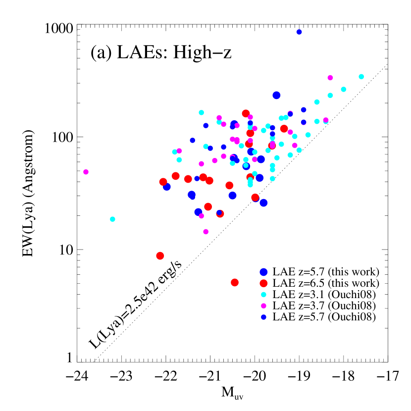
Figure 8.— EW(Ly$\alpha$) vs. $M_{\rm UV}$ for LAEs. (a) EW(Ly$\alpha$) is plotted as a function of $M_{\rm UV}$ for the $z\simeq 5.7$ and 6.5 LAEs in our sample, as well as for the $z\sim 3.1$, 3.7, and 5.7 LAEs by Ouchi et al. (2008). As for $M_{\rm UV}$, we used $M_{1500}$ listed in Table 2 for our sample. For the sample of Ouchi et al. (2008), we used the published $M_{\rm UV}$, which correspond to $M_{1300-1600}$ depending on redshift. The diagonal dotted line is defined by a limiting Ly$\alpha$ line luminosity of $2.5\times 10^{42}$ erg s^-1, which roughly corresponds to the limits of these LAE surveys. The slope of the EW(Ly$\alpha$)–$M_{\rm UV}$ correlation is largely shaped by the limiting luminosity. (b) GALEX-selected $z\simeq 0.2-0.4$ LAEs (Cowie, Barger, & Hu, 2011b) are added for comparison. $M_{\rm UV}$ was derived from the GALEX near-UV photometry in Cowie, Barger, & Hu (2010). The effective wavelength of the near-UV band is 2315.7 Å (Morrissey et al., 2007), so at redshifts $z\simeq 0.2-0.4$, the near-UV band is sampling $\sim$1650–1930 Å in the rest-frame. The near-UV, instead of the far-UV band, was used because the latter contains the redshifted Ly$\alpha$ emission. The figure indicates that the EW(Ly$\alpha$)–$M_{\rm UV}$ relation is largely shaped by the limiting luminosity.

Figure 9.— Same as Figure 8, but for LBGs from this work ($z\simeq 6$) and from Stark et al. (2010) ($z\simeq 3-6$). A number of LBGs from Stark et al. (2010) fall below the L(Ly$\alpha$)$=2.5\times 10^{42}$ erg s^-1 line, reflecting the deeper limiting Ly$\alpha$ line flux of the data. The overall distribution of the points appears similar between the LAE and LBG samples.

Figure 10.— UV continuum LFs of LAEs with $\rm EW>20$ Å at $z\simeq 5.7$ and 6.5. The thick blue and red lines represent the spatial densities of the LAEs in our sample, without incompleteness correction to $\rm EW=20$ Å. The shaded regions show the UV LFs of LAEs corrected to EW(Ly$\alpha$)$=$ 20 Å. Their lower and upper boundaries represent the lower and upper limits of the LFs. The $1\sigma$ statistical uncertainties have been included. The cyan and green curves represent the UV LFs of LBGs at $z\simeq 5.9$ and 6.8 (Bouwens et al., 2007, 2011; McLure et al., 2009; Ouchi et al., 2009). Compared to LBGs, LAEs have comparable spatial densities in the bright end, but significantly lower densities in the faint end.

Figure 11.— Normalized Ly$\alpha$ EW distribution of the LAEs in our sample. The vertical dotted lines represent the approximate EW limits for complete LAE samples at the given $M_{1500}$ ranges. We use an exponential function to fit the EW distribution. We adopt two extreme $e$-folding widths ($b=0.225$ and 0) in Section 5.3. The solid curve in the top panel is the best fit to the LAEs at $M_{1500}<-19.5$ mag (it is the same for the two cases). The dashed ($b=0.225$) and dash-dotted ($b=0$) curves in the other panels are the predicted EW distributions for the two extreme cases. The real distribution should be between the two.

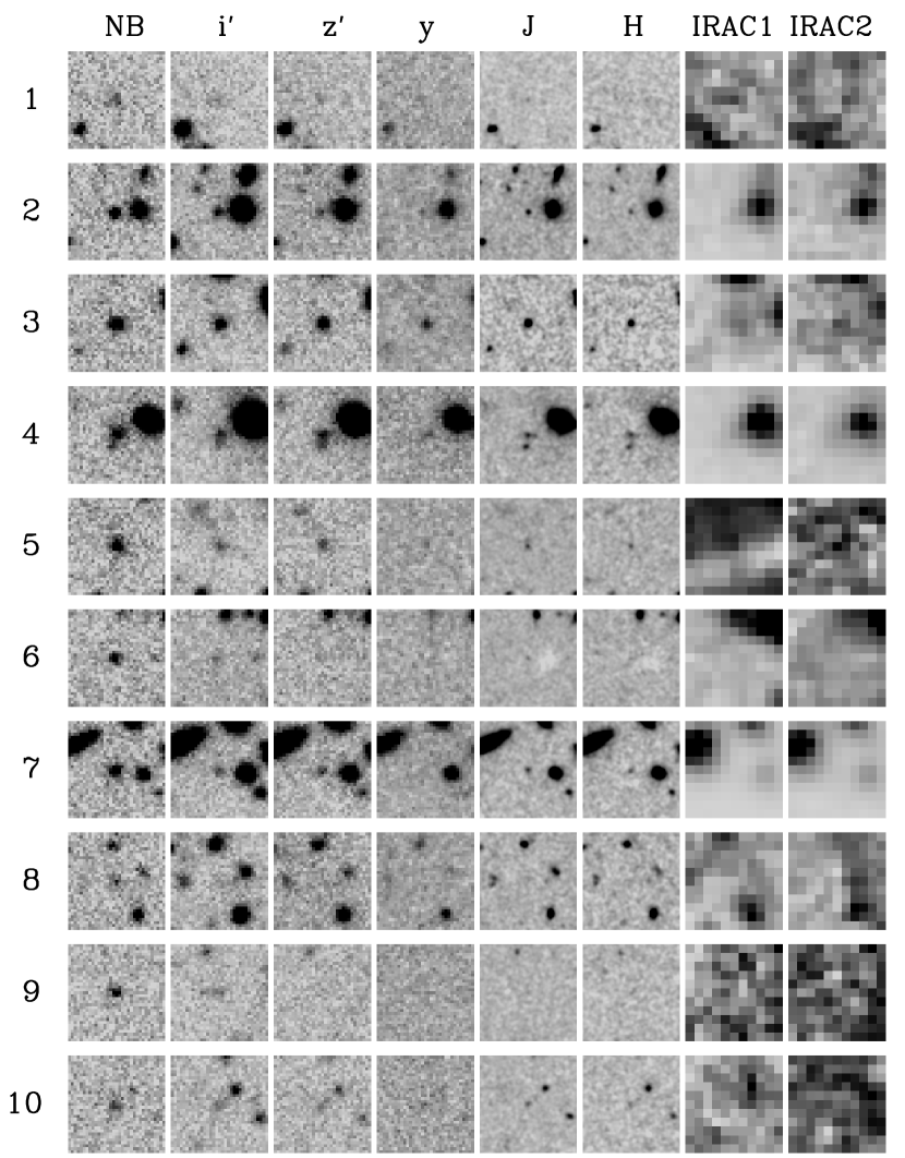
Figure 12.— Thumbnail images of the galaxies in our sample. The galaxies are in the middle of the images. The size of the images is $6\farcs 6\times 6\farcs 6$ (north is up and east to the left). An image is blank if the data is either not available or meaningless in this band.

Figure 12.— Continued.

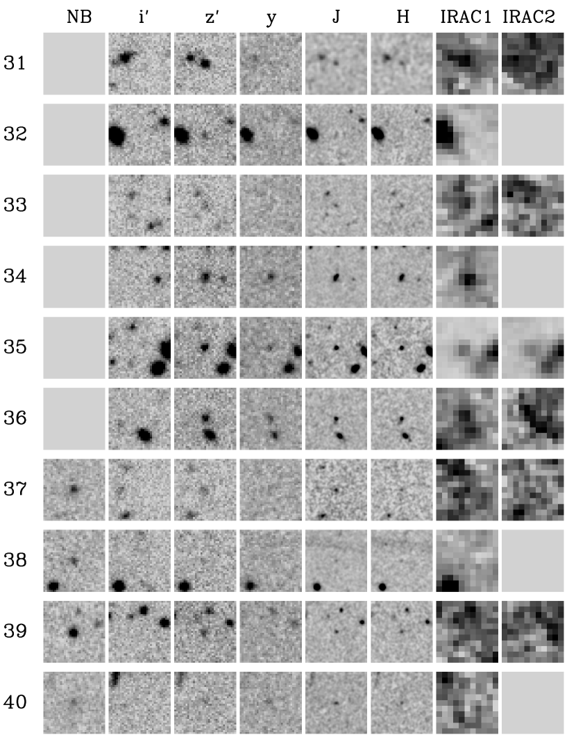
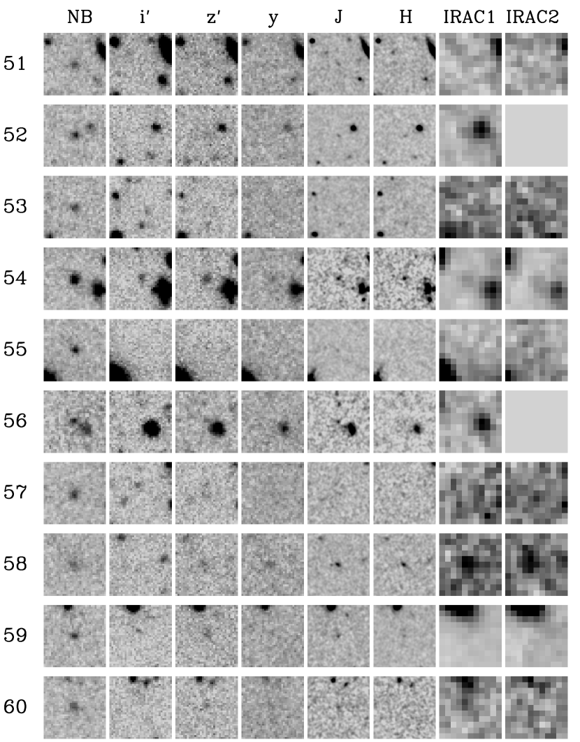
Figure 12.— Continued.

Figure 12.— Continued.

Figure 12.— Continued.

Figure 12.— Continued.

Figure 12.— Continued.

References

- Ando et al. (2006) Ando, M., Ohta, K., Iwata, I., et al. 2006, ApJ, 645, L9
- Baba et al. (2002) Baba, H., Yasuda, N., Ichikawa, S.-I., et al. 2002, Astronomical Data Analysis Software and Systems XI, 281, 298
- Bertin & Arnouts (1996) Bertin, E., & Arnouts, S. 1996, A&AS, 117, 393
- Bertin et al. (2002) Bertin, E., Mellier, Y., Radovich, M., et al. 2002, Astronomical Data Analysis Software and Systems XI, 281, 228
- Bertin (2006) Bertin, E. 2006, Astronomical Data Analysis Software and Systems XV, 351, 112
- Bradley et al. (2012) Bradley, L. D., Trenti, M., Oesch, P. A., et al. 2012, ApJ, 760, 108
- Bouwens et al. (2007) Bouwens, R. J., Illingworth, G. D., Franx, M., & Ford, H. 2007, ApJ, 670, 928
- Bouwens et al. (2009) Bouwens, R. J., Illingworth, G. D., Franx, M., et al. 2009, ApJ, 705, 936
- Bouwens et al. (2010) Bouwens, R. J., Illingworth, G. D., Oesch, P. A., et al. 2010, ApJ, 708, L69
- Bouwens et al. (2011) Bouwens, R. J., Illingworth, G. D., Oesch, P. A., et al. 2011, ApJ, 737, 90
- Bouwens et al. (2012a) Bouwens, R. J., Illingworth, G. D., Oesch, P. A., et al. 2012, ApJ, 752, L5
- Bouwens et al. (2012b) Bouwens, R. J., Illingworth, G. D., Oesch, P. A., et al. 2012, ApJ, 754, 83
- Bowler et al. (2012) Bowler, R. A. A., Dunlop, J. S., McLure, R. J., et al. 2012, MNRAS, 426, 2772
- Bunker et al. (2004) Bunker, A. J., Stanway, E. R., Ellis, R. S., & McMahon, R. G. 2004, MNRAS, 355, 374
- Bunker et al. (2010) Bunker, A. J., Wilkins, S., Ellis, R. S., et al. 2010, MNRAS, 409, 855
- Cai et al. (2011) Cai, Z., Fan, X., Jiang, L., et al. 2011, ApJ, 736, L28
- Ciardullo et al. (2012) Ciardullo, R., Gronwall, C., Wolf, C., et al. 2012, ApJ, 744, 110
- Clément et al. (2012) Clément, B., Cuby, J.-G., Courbin, F., et al. 2012, A&A, 538, A66
- Cowie, Barger, & Hu (2010) Cowie, L. L., Barger, A. J., & Hu, E. M. 2010, ApJ, 711, 928
- Cowie, Barger, & Hu (2011b) Cowie, L. L., Barger, A. J., & Hu, E. M. 2011, ApJ, 738, 136
- Cowie et al. (2011a) Cowie, L. L., Hu, E. M., & Songaila, A. 2011, ApJ, 735, L38
- Curtis-Lake et al. (2012) Curtis-Lake, E., McLure, R. J., Pearce, H. J., et al. 2012, MNRAS, 422, 1425
- Curtis-Lake et al. (2013) Curtis-Lake, E., McLure, R. J., Dunlop, J. S., et al. 2013, MNRAS, 429, 302
- Dayal & Ferrara (2012) Dayal, P., & Ferrara, A. 2012, MNRAS, 421, 2568
- de Barros et al. (2012) de Barros, S., Schaerer, D., & Stark, D. P. 2012, arXiv:1207.3663
- Dickinson et al. (2004) Dickinson, M., et al. 2004, ApJ, 600, L99
- Dijkstra et al. (2011) Dijkstra, M., Mesinger, A., & Wyithe, J. S. B. 2011, MNRAS, 414, 2139
- Dow-Hygelund et al. (2007) Dow-Hygelund, C. C., Holden, B. P., Bouwens, R. J., et al. 2007, ApJ, 660, 47
- Dunlop et al. (2012a) Dunlop, J. S., McLure, R. J., Robertson, B. E., et al. 2012, MNRAS, 420, 901
- Dunlop et al. (2012b) Dunlop, J. S., Rogers, A. B., McLure, R. J., et al. 2012, arXiv:1212.0860
- Egami et al. (2005) Egami, E., Kneib, J.-P., Rieke, G. H., et al. 2005, ApJ, 618, L5
- Ellis et al. (2013) Ellis, R. S, McLure, R. J, Dunlop, J. S, et al. 2013, ApJ, 763, L7
- Eyles et al. (2005) Eyles, L. P., Bunker, A. J., Stanway, E. R., et al. 2005, MNRAS, 364, 443
- Eyles et al. (2007) Eyles, L. P., Bunker, A. J., Ellis, R. S., et al. 2007, MNRAS, 374, 910
- Fan et al. (2001) Fan, X., Narayanan, V. K., Lupton, R. H., et al. 2001, AJ, 122, 2833
- Fan et al. (2006) Fan, X., Carilli, C. L., & Keating, B. 2006, ARA&A, 44, 415
- Finkelstein et al. (2010) Finkelstein, S. L., Papovich, C., Giavalisco, M., et al. 2010, ApJ, 719, 1250
- Finkelstein et al. (2012) Finkelstein, S. L., Papovich, C., Salmon, B., et al. 2012, ApJ, 756, 164
- Finlator et al. (2011) Finlator, K., Oppenheimer, B. D., & Davé, R. 2011, MNRAS, 410, 1703
- Finlator (2012) Finlator, K. 2012, arXiv:1203.4862
- Forero-Romero et al. (2012) Forero-Romero, J. E., Yepes, G., Gottlöber, S., & Prada, F. 2012, MNRAS, 419, 952
- Furusawa et al. (2008) Furusawa, H., Kosugi, G., Akiyama, M., et al. 2008, ApJS, 176, 1
- Garel et al. (2012) Garel, T., Blaizot, J., Guiderdoni, B., et al. 2012, MNRAS, 422, 310
- Giavalisco (2002) Giavalisco, M. 2002, ARA&A, 40, 579
- González et al. (2010) González, V., Labbé, I., Bouwens, R. J., et al. 2010, ApJ, 713, 115
- González et al. (2012) González, V., Bouwens, R., Labbe, I., et al. 2012, ApJ, 755, 148
- Grogin et al. (2011) Grogin, N. A., Kocevski, D. D., Faber, S. M., et al. 2011, ApJS, 197, 35
- Henry et al. (2012) Henry, A. L., Martin, C. L., Dressler, A., Sawicki, M., & McCarthy, P. 2012, ApJ, 744, 149
- Hibon et al. (2010) Hibon, P., et al. 2010, A&A, 515, 97
- Hu et al. (2002) Hu, E. M., Cowie, L. L., McMahon, R. G., et al. 2002, ApJ, 568, L75
- Hu et al. (2010) Hu, E. M., Cowie, L. L., Barger, A. J., et al. 2010, ApJ, 725, 394
- Hsieh et al. (2012) Hsieh, B.-C., Wang, W.-H., Yan, H., et al. 2012, ApJ, 749, 88
- Iye et al. (2006) Iye, M., Ota, K., Kashikawa, N., et al. 2006, Nature, 443, 186
- Jiang et al. (2011) Jiang, L., Egami, E., Kashikawa, N., et al. 2011, ApJ, 743, 65
- Kashikawa et al. (2004) Kashikawa, N., Shimasaku, K., Yasuda, N., et al. 2004, PASJ, 56, 1011
- Kashikawa et al. (2006) Kashikawa, N., Shimasaku, K., Malkan, M. A., et al. 2006, ApJ, 648, 7
- Kashikawa et al. (2011) Kashikawa, N., Shimasaku, K., Matsuda, Y., et al. 2011, ApJ, 734, 119
- Kennicutt (1998) Kennicutt, R. C., Jr. 1998, ARA&A, 36, 189
- Kodaira et al. (2003) Kodaira, K., Taniguchi, Y., Kashikawa, N., et al. 2003, PASJ, 55, L17
- Koekemoer et al. (2002) Koekemoer, A. M., Fruchter, A. S., Hook, R. N., & Hack, W. 2002, The 2002 HST Calibration Workshop : Hubble after the Installation of the ACS and the NICMOS Cooling System, 337
- Koekemoer et al. (2011) Koekemoer, A. M., Faber, S. M., Ferguson, H. C., et al. 2011, ApJS, 197, 36
- Komatsu et al. (2011) Komatsu, E., Smith, K. M., Dunkley, J., et al. 2011, ApJS, 192, 18
- Krug et al. (2012) Krug, H. B., Veilleux, S., Tilvi, V., et al. 2012, ApJ, 745, 122
- Laporte et al. (2012) Laporte, N., Pelló, R., Hayes, M., et al. 2012, A&A, 542, L31
- Lorenzoni et al. (2011) Lorenzoni, S., Bunker, A. J., Wilkins, S. M., et al. 2011, MNRAS, 414, 1455
- Madau et al. (1998) Madau, P., Pozzetti, L., & Dickinson, M. 1998, ApJ, 498, 106
- Magee et al. (2007) Magee, D. K., Bouwens, R. J., & Illingworth, G. D. 2007, in ASP Conf. Ser. 376, Astronomical Data Analysis Software and Systems XVI, ed. R. A. Shaw, F. Hill, & D. J. Bell (San Francisco: ASP), 261
- McLure et al. (2009) McLure, R. J., Cirasuolo, M., Dunlop, J. S., Foucaud, S., & Almaini, O. 2009, MNRAS, 395, 2196
- McLure et al. (2010) McLure, R. J., Dunlop, J. S., Cirasuolo, M., et al. 2010, MNRAS, 403, 960
- McLure et al. (2011) McLure, R. J., Dunlop, J. S., de Ravel, L., et al. 2011, MNRAS, 418, 2074
- Morrissey et al. (2007) Morrissey, P., et al. 2007, ApJS, 173, 682
- Nagao et al. (2004) Nagao, T., Taniguchi, Y., Kashikawa, N., et al. 2004, ApJ, 613, L9
- Nagao et al. (2005) Nagao, T., Kashikawa, N., Malkan, M. A., et al. 2005, ApJ, 634, 142
- Nagao et al. (2007) Nagao, T., Murayama, T., Maiolino, R., et al. 2007, A&A, 468, 877
- Nilsson et al. (2009) Nilsson, K. K., Möller-Nilsson, O., Møller, P., Fynbo, J. P. U., & Shapley, A. E. 2009, MNRAS, 400, 232
- Oesch et al. (2010) Oesch, P. A., Bouwens, R. J., Illingworth, G. D., et al. 2010, ApJ, 709, L16
- Oesch et al. (2012) Oesch, P. A., Bouwens, R. J., Illingworth, G. D., et al. 2012, ApJ, 759, 135
- Oke & Gunn (1983) Oke, J. B., & Gunn, J. E. 1983, ApJ, 266, 713
- Ono et al. (2010) Ono, Y., Ouchi, M., Shimasaku, K., et al. 2010, ApJ, 724, 1524
- Ono et al. (2012) Ono, Y., Ouchi, M., Mobasher, B., et al. 2012, ApJ, 744, 83
- Osterbrock et al. (1989) Osterbrock, D. E. 1989, Astrophysics of Gaseous Nebulae and Active Galactic Nuclei (Mill Valley, CA: Univ. Science Books)
- Ota et al. (2008) Ota, K., Kashikawa, N., Malkan, M. A., et al. 2008, arXiv:0804.3448
- Ota & Iye (2012) Ota, K., & Iye, M. 2012, MNRAS, 423, 444
- Ouchi et al. (2004) Ouchi, M., Shimasaku, K., Okamura, S., et al. 2004, ApJ, 611, 660
- Ouchi et al. (2008) Ouchi, M., Shimasaku, K., Akiyama, M., et al. 2008, ApJS, 176, 301
- Ouchi et al. (2009) Ouchi, M., Mobasher, B., Shimasaku, K., et al. 2009, ApJ, 706, 1136
- Ouchi et al. (2010) Ouchi, M., Shimasaku, K., Furusawa, H., et al. 2010, ApJ, 723, 869
- Pentericci et al. (2011) Pentericci, L., Fontana, A., Vanzella, E., et al. 2011, ApJ, 743, 132
- Pirzkal et al. (2007) Pirzkal, N., Malhotra, S., Rhoads, J. E., & Xu, C. 2007, ApJ, 667, 49
- Pirzkal et al. (2012) Pirzkal, N., Rothberg, B., Nilsson, K. K., et al. 2012, ApJ, 748, 122
- Reddy et al. (2008) Reddy, N. A., Steidel, C. C., Pettini, M., et al. 2008, ApJS, 175, 48
- Rhoads et al. (2004) Rhoads, J. E., Xu, C., Dawson, S., et al. 2004, ApJ, 611, 59
- Rhoads et al. (2012) Rhoads, J. E., Hibon, P., Malhotra, S., Cooper, M., & Weiner, B. 2012, ApJ, 752, L28
- Robertson et al. (2010) Robertson, B. E., Ellis, R. S., Dunlop, J. S., McLure, R. J., & Stark, D. P. 2010, Nature, 468, 49
- Schaerer & de Barros (2010) Schaerer, D., & de Barros, S. 2010, A&A, 515, A73
- Schenker et al. (2012) Schenker, M. A., Stark, D. P., Ellis, R. S., et al. 2012, ApJ, 744, 179
- Shapley et al. (2003) Shapley, A. E., Steidel, C. C., Pettini, M., & Adelberger, K. L. 2003, ApJ, 588, 65
- Shibuya et al. (2012) Shibuya, T., Kashikawa, N., Ota, K., et al. 2012, ApJ, 752, 114
- Shimasaku et al. (2006) Shimasaku, K., Kashikawa, N., Doi, M., et al. 2006, PASJ, 58, 313
- Silva et al. (2013) Silva, M., Santos, M. G., Gong, Y., & Cooray, A. 2013, ApJ, 763, 132
- Stark et al. (2010) Stark, D. P., Ellis, R. S., Chiu, K., Ouchi, M., & Bunker, A. 2010, MNRAS, 408, 1628
- Stark et al. (2011) Stark, D. P., Ellis, R. S., & Ouchi, M. 2011, ApJ, 728, L2
- Stark et al. (2013) Stark, D. P., Schenker, M. A., Ellis, R. S., et al. 2013, ApJ, 763, 129
- Steidel & Hamilton (1993) Steidel, C. C., & Hamilton, D. 1993, AJ, 105, 2017
- Taniguchi et al. (2005) Taniguchi, Y., Ajiki, M., Nagao, T., et al. 2005, PASJ, 57, 165
- Tilvi et al. (2010) Tilvi, V., Rhoads, J. E., Hibon, P., et al. 2010, ApJ, 721, 1853
- Toshikawa et al. (2012) Toshikawa, J., Kashikawa, N., Ota, K., et al. 2012, ApJ, 750, 137
- Vanzella et al. (2011) Vanzella, E., Pentericci, L., Fontana, A., et al. 2011, ApJ, 730, L35
- van Dokkum (2001) van Dokkum, P. G. 2001, PASP, 113, 1420
- Walter et al. (2012) Walter, F., Decarli, R., Carilli, C., et al. 2012, ApJ, 752, 93
- Wilkins et al. (2010) Wilkins, S. M., Bunker, A. J., Ellis, R. S., et al. 2010, MNRAS, 403, 938
- Wilkins et al. (2011) Wilkins, S. M., Bunker, A. J., Stanway, E., Lorenzoni, S., & Caruana, J. 2011, MNRAS, 417, 717
- Willott et al. (2013) Willott, C. J., McLure, R. J., Hibon, P., et al. 2013, AJ, 145, 4
- Windhorst et al. (2011) Windhorst, R. A., et al. 2011, ApJS, 193, 27
- Yagi et al. (2002) Yagi, M., Kashikawa, N., Sekiguchi, M., et al. 2002, AJ, 123, 66
- Yajima et al. (2012) Yajima, H., Li, Y., Zhu, Q., & Abel, T. 2012, MNRAS, 424, 884
- Yan & Windhorst (2004) Yan, H., & Windhorst, R. A. 2004, ApJ, 612, L93
- Yan et al. (2005) Yan, H., Dickinson, M., Stern, D., et al. 2005, ApJ, 634, 109
- Yan et al. (2006) Yan, H., Dickinson, M., Giavalisco, M., et al. 2006, ApJ, 651, 24
- Yan et al. (2010) Yan, H., Windhorst, R., Hathi, N., et al. 2010, Res. Astron. Astrophys., 10, 867
- Zheng et al. (2010) Zheng, Z., Cen, R., Trac, H., & Miralda-Escudé, J. 2010, ApJ, 716, 574