Modeling the transport of interacting matter-waves in disorder by a nonlinear diffusion equation

Abstract

We model the expansion of an interacting atomic Bose-Einstein condensate in a disordered lattice with a nonlinear diffusion equation normally used for a variety of classical systems. We find approximate solutions of the diffusion equation that well reproduce the experimental observations for both short and asymptotic expansion times. Our study establishes a connection between the peculiar shape of the expanding density profiles and the microscopic nonlinear diffusion coefficients.

I Introduction

The interplay of disorder and interactions in quantum systems gives rise to a variety of interesting phenomena, ranging from glassy quantum phases to non-standard transport properties. In particular, interactions are known to be able to break the Anderson localization due to disorder, restoring transport in otherwise insulating systems. The prototypal systems in which such effect has been studied are one-dimensional disordered potentials, where the expansion dynamics of an initially localized wavepacket has been extensively investigated both in theory Shepe93 ; Kopidakis08 ; Pikovsky08 ; Flach09 ; Skokos09 ; Veksler09 ; Mulansky10 ; Laptyeva10 ; Iomin10 ; Min ; Larcher09 and experiments Lucioni11 . There is now a general agreement on an anomalous diffusion process, where the time-exponent of the expansion is smaller than the one found in linear systems, e.g. $<x^{2}>\sim t^{\alpha}$, with $\alpha<1$. This subdiffusion is essentially due to the presence of a local diffusion coefficient that depends on density and therefore decreases as the wavepacket expands. While the time-evolution of the second moment of the distribution observed in numerics and experiments agrees with microscopic models, a satisfying modeling of the evolution of the overall shape of the wavepacket is still missing. A natural question is whether this expansion process can be modeled with a nonlinear diffusion equation widely employed to describe related transport processes in classical systems Leibenzon ; Ames , which contains explicitly a density-dependent diffusion coefficient Mulansky11 ; Mulansky12 ; Laptyeva12 ; Cherroret . Recent numerical studies have indeed established a link between the nonlinear diffusion equation (NDE) and the asymptotic regime of subdiffusion, employing known self-similar solutions of the NDE Mulansky12 ; Laptyeva12 . However, a comparison with experimental data is not yet possible, since these solutions do not apply to the limited time interval that is possible to study in experiments, where normally the shape of the wavepacket changes with time Lucioni11 .

In this work we study this problem and derive approximate solutions of the NDE for the short-time regime accessible in experiments. We find a relatively good agreement between the density distributions measured in the experiment and these solutions, and we identify a time-dependent exponent that links the evolution of the second moment to the changing shape of the distribution. While the present experiments lack the necessary spatial resolution, we find that the detailed study of such shape can give direct evidence of the exponent of nonlinearity of the local diffusion coefficient.

II The disordered, interacting system

In the experiment we employ an ultracold cloud on weakly-interacting bosons in a one-dimensional optical lattice that mimics a truly disordered potential. More in detail, we realize a quasiperiodic lattice by perturbing a strong sinusoidal lattice with a secondary one having an incommensurate spacing. As described in more detail elsewhere Lucioni11 ; Modugno09 , non-interacting particles in such potential can be described by the well-known Aubry-André tight-binding (single band) Hamiltonian Aubry :

$$H=-J\sum_{j}(b^{\dagger}_{j}b_{j+1}+b^{\dagger}_{j+1}b_{J})+\Delta\sum_{j}\cos(2\pi\beta j)n_{j}\,,$$ (1)

where $b^{\dagger}_{j},b_{j}$ and $n_{j}=b^{\dagger}_{j}b_{j}$ are the standard on-site creation, destruction and number bosonic operators, $J$ is the kinetic (hopping) energy, $\Delta$ is the quasi-disorder energy and $\beta$ is the ratio of the two lattice spacings. This model is known to show Anderson localization for $\Delta>2J$, with an essentially energy-independent localization length $\xi\sim 1/\ln(\Delta/2J)$, in units of the main lattice spacing Roati08 .

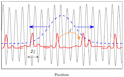
Figure 1: (color online) Schematic representation of the disordered, interacting system. An initial non-interacting wavepacket (blue dashed line) can be decomposed into exponentially-localized single-particle states (red thick lines) of the quasiperiodic lattice (grey thin line). A weak interaction couples the states with a density-dependent rate $\Gamma$ and allows an expansion of the wavepacket. Only states separated by one quasiperiod, 1/($\beta$-1), are shown for clarity.

In the experiment we can realize this single-particle regime, and also add a controllable repulsive interaction between the particles, by employing potassium-39 atoms with a magnetically-tunable Feshbach resonance Roati07 ; Derrico07 . In presence of interaction, one needs to introduce an additional term in the Hamiltonian

$$H_{int}=U\sum_{j}n_{j}(n_{j}-1)\,,$$ (2)

where $U$ parameterizes the two-particles interaction energy and $E_{int}\sim Un(x,t)$ represents the local interaction per particle, where $n(x,t)$ is the time-dependent density distribution. Such interaction can couple distinct single-particle localized states, allowing for macroscopic transport. To probe the transport properties in the experiment, we initially prepare a low-temperature sample in the combined potential of a quasi-periodic lattice with $\Delta>2J$ and a harmonic trap, characterized by a Gaussian density distribution $n(x)$. We then remove suddenly the trap, and let the sample expand along the lattice for a variable time, in presence of an additional radial confinement. In Fig.1 we show a schematic representation of the experiment. As shown in Fig.2, we essentially observe no expansion if $U$=0, while for finite $U$ the distribution broadens and changes shape with increasing time. The square root of the second moment of $n(x,t)$ increases with a subdiffusive behavior of the kind

$$\sigma(t)=\sqrt{\langle x^{2}\rangle}=\sigma_{0}(1+t/t_{0})^{\alpha}\,,$$ (3)

with a characteristic exponent $\alpha$ in the range 0.2-0.4 for $E_{int}\lesssim J$ as already discussed in ref.Lucioni11 (we do not consider the regime of $E_{int}\gg J$, where self-trapping phenomena can complicate the dynamics). While the subdiffusive expansion of the width can be explained with heuristic models of the microscopic dynamics Lucioni11 ; Aleiner , little or no analysis is available for the evolution of the overall shape of $n(x,t)$.

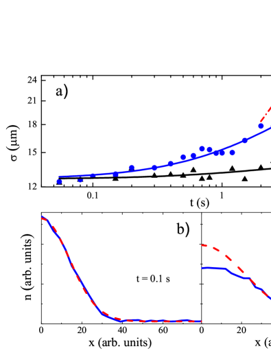
Figure 2: (color online) a) Time evolution of the width of the atomic distribution for strong (blue dots) and very weak (black triangles) interaction. The continuous lines are fits with Eq.(3) and give $\alpha$ exponents of $0.28\pm 0.02$ and $0.04\pm 0.02$ respectively; the dash-dotted line represents the asymptotic slope expected for normal diffusion. The initial Gaussian distribution (b) evolves into a flat-top distribution at longer times (c). The dashed lines are Gaussian fits of the tails of the distributions.

Let us start discussing a simple model of the microscopic dynamics which applies to the regime of weak interactions, where one can still describe the many body-states as superposition of few single-particle states. A general expectation is that a local diffusion coefficient can be defined as $D\sim\Gamma\xi^{2}$, where $\xi$ is the single-particle localization length and $\Gamma$ is the coupling rate of single-particle states by the interaction. The latter can be evaluated in perturbation theory as

$$\Gamma_{if}=\frac{2\pi}{\hbar}\frac{|\langle i|H_{int}|f\rangle|^{2}}{|E_{i}-E_{f}|}\,.$$ (4)

where $|i\rangle$ and $|f\rangle$ are two generic initial and final states (they actually represents quadruplets of single-particle states, because of the form of $H_{int}$) and $|E_{i}-E_{f}|$ is their energy separation, which is of the order of $\Delta$. Such coupling is possible only if $\langle i|H_{int}|f\rangle>|E_{i}-E_{f}|$. One can have two different scenarios. If $E_{int}\sim\Delta$, the dominant couplings are within nearby states, and one finds that $\langle i|H_{int}|f\rangle$ is essentially $E_{int}I_{if}$, where $I_{if}$ is an overlap integral of the order unity. This implies that $D\propto n(x,t)^{2}$ and, since in 1D $n\sim 1/\sigma$, that $D\propto\sigma^{-2}$. If instead $E_{int}\ll\Delta$, only long-distance couplings are possible, which tend to decrease with decreasing interaction energy. In this case one must expect $D\propto n(x,t)^{\beta}\propto\sigma^{-\beta}$, with $\beta>2$.

By solving the standard diffusion equation

$$\frac{\partial n(x,t)}{\partial t}=D\frac{\partial^{2}n(x,t)}{\partial x^{2}}$$ (5)

for the width of the distribution, $d\sigma^{2}(t)/dt=2D$, one finds a time dependence for $\sigma(t)$ of the form of Eq.(3), with $\alpha=1/2$. If the diffusion coefficient depends on the width itself as $D\propto\sigma^{-\beta}$, Eq.(3) continues to describe the time evolution of the width but with a time exponent $\alpha=1/(2+\beta)$. These simple expectations match what has been observed in experiments Lucioni11 and numerical calculations (e.g. Ref. Larcher12 and references therein) for the evolution of $\sigma(t)$.

III The nonlinear diffusion equation

Let us now turn our attention to the evolution of the shape of $n(x,t)$. The idea is to start from a nonlinear diffusion equation (NDE) of the form

$$\frac{\partial n(x,t)}{\partial t}=\frac{\partial}{\partial x}\Bigl{(}D_{0}n^{a}(x,t)\frac{\partial n(x,t)}{\partial x}\Bigr{)}\,,$$ (6)

which takes explicitly into account a density-dependent diffusion coefficient. The NDE is usually studied in the asymptotic limit, where a self-similar solution exists Tuck76 :

$$n(x,t)\propto\begin{cases}\Bigl{(}1-\frac{x^{2}}{w(t)^{2}}\Bigr{)}^{1/a}&\mbox{for }|x|<w(t)\\ 0\,&\mbox{for }|x|>w(t)\end{cases}$$ (7)

The front of the diffusion $w(t)$ has the time dependence $w(t)\propto t^{1/(2+a)}$, and the same dependence is found for $\sigma(t)$. In our specific problem we expect an exponent $a\geq 2$; for $a=2$ it is exactly an inverted parabola.

This self-similar solution obviously cannot reproduce our short-time expansion, where we clearly see a changing shape of the distribution. As shown in Fig.2, in the experiment $n(x)$ is initially Gaussian, while later it develops a flatter top and a relatively faster decay of the tails. This general behavior is actually consistent with the picture of a density-dependent diffusion coefficient discussed above, which predicts a larger $D$ at the center of the distribution, and a reduced one in the tails.

We therefore look for an approximate solution of the NDE which can interpolate between the initial Gaussian distribution and the asymptotic regime. One can start by noting that a Gaussian can be obtained as a limit of a slightly different version of Eq.(7)

$$e^{-x^{2}/w^{2}}=\lim_{b\rightarrow 0}\Bigl{(}1-\frac{bx^{2}}{w^{2}}\Bigr{)}^{1/b}\,.$$ (8)

The conjecture is then that a solution of the form

$$n(x,t)=\begin{cases}A\Bigl{(}1-\frac{b(t)x^{2}}{w(t)^{2}}\Bigr{)}^{1/b(t)}&|x|<w(t)/\sqrt{b(t)}\\ 0\,&|x|\geq w(t)/\sqrt{b(t)}\end{cases}$$ (9)

might reproduce the short-time regime of the true solution of the NDE. Here $A=A(b,w)$ is an appropriate normalization coefficient, and

$$b(t)=a(1-\exp(-t/\tau))$$ (10)

is a time-dependent exponent. To verify this conjecture, we solve numerically Eq.(6) for various values of the nonlinear diffusion exponent $a$, with an initial Gaussian distribution, and we compare the calculated $n(x,t)$ with the approximation above. As summarized in Fig.3, we find that this approximation works reasonably well at all times, for values of the nonlinear diffusion exponent in the range $a=1-3$ (see Appendix B for more details). In particular, the numerical $n(x)$ is reasonably well reproduced by Eq.(9), besides a limited deviation of the tails. As we will discuss later, this deviation is not an issue in the analysis of the experimental data, which has however a limited resolution. There is also a good agreement of the time evolution of the width with Eq.(3), for an exponent $\alpha$ that is consistent with $\alpha=1/(a+2)$. Finally, $b(t)$ is reasonably well fitted by Eq.(10).

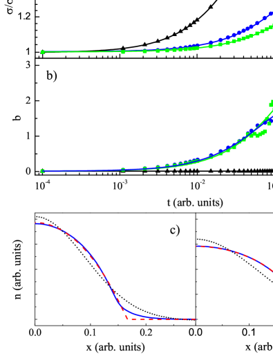
Figure 3: (color online) a) Time evolution of the width of the numerical solution of the NDE (6) for $a=0$ (black triangles), $a=2$ (blue dots) and $a=3$ (green squares). Lines are fits with Eq.(3) and give $\alpha$ exponents of 0.5, 0.24 and 0.18, respectively. b) Time evolution of the time-dependent exponent $b$, with same color and symbol scheme as above. Lines are fits with Eq.(10). c) Fit of the numerical solution of the NDE for $a=2$ (blue continuous) with Eq.(9) (red dashed) or a Gaussian (black dotted) for $t$=0.01; d) same as above, for $t$=0.1.

IV Experimental results

We can now use Eq.(9) to fit the experimental profiles. Fig.4 shows the results for a set of experimental data with a mean initial interaction energy $E_{int}=2.3J$ (blue data in Fig.2), with a rather good agreement. We find that $b$ is close to 0 for short expansion times (Fig.4a) and evolves to larger values for increasing expansion times as the flat-top distribution appears (Fig.4b). The goodness of the fit for varying time can be evaluated by the coefficient of determination $R^{2}$. Fig.4c shows the evolution of $R^{2}$ for both a Gaussian fit and the fit with the approximate solution of the NDE: while the fit with the Gaussian gets worse as the atomic cloud expands, the fit with Eq.(9) remains constantly good. We note that when the interaction energy is not strong enough to allow the atomic cloud expansion (black data in Fig.2), we cannot appreciate a variation of the the shape of $n(x)$, which is always well fitted by a Gaussian.

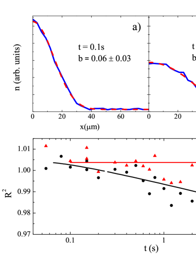
Figure 4: (color online) a,b) Fit of the experimental profiles (blue continuous line) with Eq.(9) (red dashed line). The initial Gaussian distribution (a) is well fitted with $b\approx 0$, while at longer times (b) the exponent increases. c) Coefficient of determination $R^{2}$ for a fit with Eq.(9) (red triangles) and for a Gaussian fit (black dots). The lines are a guide to the eye.

We can now compare the evolution of the exponents $b$ for the experiment and the numerical solution of the NDE. A direct comparison can be obtained by studying the evolution of $b$ as a function of the rescaled width $\sigma(t)/\sigma_{0}$, as shown for example in Fig.5. This allows to get rid of the different time and width scales in the experiment and in the simulations. The experimental data refer to the same set of Fig.4, for which we measured $\alpha=0.28\pm 0.02$, it is therefore natural to compare it with the solution of the NDE for $a=2$. One can note a qualitatively similar behavior of theory and experiment, with an initial $b\approx 0$ that increases towards an asymptotic value. However, the asymptotic value for the experiment is not the expected one, and the overall evolution is apparently slower.

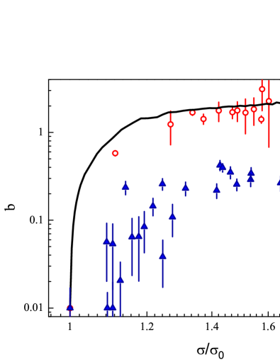
Figure 5: (color online) Evolution of the exponent $b$ with the rescaled width obtained by fitting $n(x,t)$ with the approximate solution of the NDE: experiment (blue triangles) numerical solution of the NDE with $a=2$ (black line), numerical solution of the DNLSE (red circles).

We attribute this discrepancy to the finite spatial resolution with which the experimental $n(x)$ is detected. Actually, for our imaging system we have a Gaussian point spread function with a width of $\sigma_{I}$=10$\mu$m, which is therefore comparable to the initial width $\sigma_{0}$. The expected effect of such finite resolution is indeed a smoothing of the steep decay of the tails of $n(x)$, and therefore a decrease of the measured exponent $b$. A comparison of the numerical and experimental profiles in Figs.3-4 confirms this argument.

A more quantitative comparison can be made by properly taking the finite resolution into account. To strengthen our analysis, we also performed a numerical simulation of the expansion by employing a one-dimensional discrete non-linear Schrödinger equation (DNLSE) that is known to reproduce the evolution of our type of disordered system in the regime of weak interaction. One example of the numerical $n(t)$ for a long expansion time is shown in Fig.6. In absence of a finite spatial resolution (Fig.6a), one notes rather steep tails that can indeed be fitted with the approximate solution of the NDE with an exponent $b\approx 2$. Actually, the full evolution of $b(t)$ for the solution of the DNLSE, which is also reported in Fig.5, shows a rather good agreement with the solution of the NDE at all times. When instead the distribution is convolved with the calculated Gaussian transfer function (Fig.6b), one can observe a clear smoothing of the tails, leading to a substantial reduction of $b$.

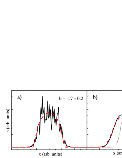
Figure 6: (color online) Effect of the finite imaging resolution on the numerical simulations with the DNLSE. a) $n(x)$ after a large expansion time (black continuous line), in absence of a finite resolution, fitted by Eq.(9) (red dashed line). b) the same $n(x)$ after convolution with Gaussian transfer function (gray dotted line).

A direct comparison of the experiment with the NDE can therefore be made only by properly taking into account such finite resolution also in the numerical solution of the NDE. Fig.7 compares the exponent $b$ from the experiment with those fitted from the numerical solutions of both NDE and DNLSE, convolved with the Gaussian point-spread function. The evolution of the NDE exponent is now slower, and rather close to the experimental one. Clearly, the asymptotic value $b=a$ can be reached only if the width of the distribution becomes much larger than $\sigma_{I}$.

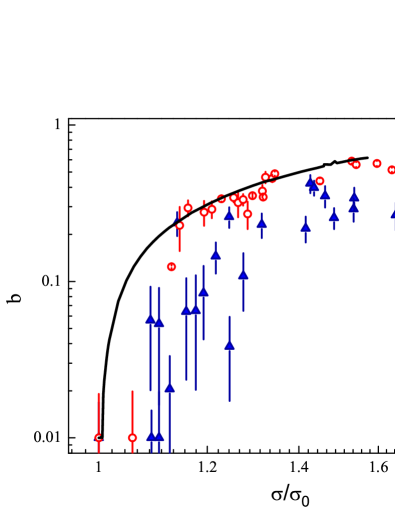
Figure 7: (color online) Evolution of the exponent $b$ with the rescaled width obtained by fitting $n(x,t)$, taking into account the finite spatial resolution: experiment (blue triangles), numerical solution of the NDE with $a=2$ (black line), numerical solution of the DNLSE (red circles).

The specific set of experimental data we have discussed so far is just one example. We have actually found similar results for other values of the initial interaction energy in the range $E_{int}$=0.5-3$J$. For weaker interactions, although a small expansion can be detected in the experiment (see for example the data in Fig.2), the shape stays essentially Gaussian up to the longest observation time. We speculate that other effects existing in the experimental setups, such as a weak time-dependent noise, might be responsible for this observationDerrico13 .

V Conclusions

In conclusion, we have compared the evolution of the density distribution during the subdiffusive expansion of interacting atoms in disorder with the solution of a general non-linear diffusion equation of the form of Eq.(6). In this equation the local diffusion coefficient is considered to be proportional to the density to some power $a$. To account for the relatively small timescales available in experiments, we have built an approximate solution of the nonlinear diffusion equation that provides a sufficiently accurate interpolation between the initial Gaussian wavepacket and the asymptotic distribution, which is characterized by steep tails. We can see a qualitative agreement on the evolution of the shape of the distribution, which confirms the hypothesis of a microscopic density-dependent diffusion coefficient. The finite experimental spatial resolution did not so far allow us to verify the expected relation between the spatial and time exponents. This might however be explored in future experiments having state-of-the-art spatial resolution.

VI Appendices

VI.1 Experimental methods and parameters

The quasiperiodic potential is created by perturbing a deep optical lattice with a weaker lattice of incommensurate wavelength: $V(x)$=$V_{1}\cos^{2}(k_{1}x)+V_{2}\cos^{2}(k_{2}x+\phi)$. Here $k_{i}$=$2\pi/\lambda_{i}$ are the wavevectors of the lattices, with $\lambda_{1}$=1064.4 nm and $\lambda_{2}$=859.6 nm, giving a ratio $\beta$=1.238…, $\phi$ is the relative phase between the two lattices. The main lattice fixes the lattice spacing, $d$=$\lambda_{1}/2$, and the tunneling energy $J$. The quasi-disorder strength, $\Delta$, scales linearly with the secondary lattice strength $V_{2}$ Modugno09 .

The atomic sample consists in a Bose-Einstein condensate of ³⁹K atoms in their ground state, whose $s$-wave scattering length $a_{s}$ can be adjusted from about zero to large positive values thanks to a broad magnetic Feshbach resonance Roati07 ; Derrico07 . The condensate is initially produced in a crossed optical trap at $a_{s}=280a_{0}$, and contains about $4\times 10^{4}$ atoms. A quasiperiodic lattice with $\Delta\approx 3J$ is then slowly added. The radial confinement induced by the optical trap and the lattice beams is $\omega_{r}\approx 2\pi\times 80$ Hz while the axial one is $\omega_{ax}\approx 2\pi\times 70$ Hz.

At a given time, $t=0$, the optical trap is suddenly switched off and the atoms are let free to expand along the lattice, in presence of a radial confinement of $\omega_{r}\approx 2\pi\times 50$ Hz given by the radial profile of the lattice beam. At the same time, $\Delta$ and $a$ are tuned to their final values within $10$ ms, and kept there for the rest of the evolution. The interaction parameter is set by the scattering length as

$$U=\frac{2\pi\hbar^{2}a_{s}}{m}\int\varphi^{4}d^{3}x\,,$$ (11)

where $\varphi$ is the 3D single-particle Wannier wavefunction. A maximum $E_{int}\approx J$ can be realized, since an increasing repulsion tends to broaden the system radially, thus reducing its density.

The atomic density distribution is detected via absorption imaging, and integrated along the radial direction to obtain the one-dimensional profiles $n(x)$.

VI.2 Approximate solution of the nonlinear diffusion equation

The complete expression for the approximation to the solutions of the NDE, normalized to unity, is

$$n(x,t)=\frac{b^{3/2}\Gamma(1/b+3/2)}{\sqrt{\pi}w\Gamma(1/b)}\Bigl{(}1-\frac{bx^{2}}{w^{2}}\Bigr{)}^{1/b}\,,$$ (12)

for $|x|<w/\sqrt{b}$, and zero otherwise. This expression provides an overall better fit of the numerical solutions of the NDE in all time regimes than either a Gaussian or the asymptotic solution of the NDE. Fig.8 shows for example the coefficient of determination for the specific case of $a=2$.

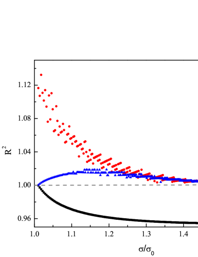
Figure 8: (color online) Coefficient of determination $R^{2}$ of the fit of the numerical solutions of the NDE with Eq.(12) (blue triangles), with a Gaussian (black squares) or with Eq.(7) (red dots).

VI.3 Numerical simulations

The DNLSE studied in the numerical simulations reproduces the experimental system in the limit of negligible population of the radial degrees of freedom:

$$i\frac{d}{dt}\psi_{j}(t)=-(\psi_{j+1}(t)+\psi_{j-1}(t))+$$

$$+\Delta/J\sin(2\pi\beta j+\phi)|\psi_{j}(t)|^{2}+\gamma|\psi_{j}|^{2}\psi_{j}\,.$$ (13)

Here $\psi_{j}(t)$ are the coefficients of the wave function in the Wannier basis, normalized in such a way that their squared modulus corresponds to the atom density on the j-th site of the lattice. The mean field interaction strength is given by $\gamma$. The relation between $E_{int}$ and $\gamma$ is approximately $E_{int}\approx 2J\gamma/\bar{n}_{s}$, where $\bar{n}_{s}$ is the mean number of sites occupied by the atomic distribution. The initial condition of the simulations is a Gaussian distribution as in the experiment. For each expansion time, $n(x)$ is obtained by averaging the profiles resulting from 100 different realizations of the quasiperiodic potential with randomly varied phase $\phi$ in the range $[0,2\pi]$. The specific results of Figs.5-7 where obtained with parameters $\gamma=40$ and $\Delta/J=2.5$

VII Acknowledgments

This work was motivated by an initial suggestion by Sergej Flach. We acknowledge support by the European Research Council (grants 203479, QUPOL and 247371, DISQUA), and the Italian Ministry for Research (PRIN 2009).

References

- (1) D. L. Shepelyansky, Phys. Rev. Lett. 70, 1787 (1993).
- (2) G. Kopidakis, S. Komineas, S. Flach, and S. Aubry, Phys. Rev. Lett. 100, 084103 (2008).
- (3) A. S. Pikovsky, D. L. Shepelyansky, Phys. Rev. Lett. 100, 094101 (2008).
- (4) S. Flach, D. O. Krimer, C. Skokos, Phys. Rev. Lett. 102, 024101 (2009).
- (5) C. Skokos, D. O. Krimer, S. Komineas, and S. Flach, Phys. Rev. E 79, 056211 (2009).
- (6) H. Veksler, Y. Krivolapov, S. Fishman, Phys. Rev. E 80, 037201 (2009).
- (7) M. Mulansky, A. Pikovsky, Europhys. Lett. 90, 10015 (2010).
- (8) T. V. Laptyeva, J. D. Bodyfelt, D. O. Krimer, Ch. Skokos, and S. Flach, Europhys. Lett. 91, 30001 (2010).
- (9) A. Iomin, Phys. Rev. E 81, 017601 (2010).
- (10) B.Min, T. Li, M. Rosenkranz, and W. Bao, Phys. Rev. A 86, 053612 (2012).
- (11) M. Larcher, F. Dalfovo, M. Modugno, Phys. Rev. A 80, 053606 (2009).
- (12) E. Lucioni, B. Deissler, L. Tanzi, G. Roati, M. Zaccanti, M. Modugno, M. Larcher, F. Dalfovo, M. Inguscio, G. Modugno, Phys. Rev. Lett. 106, 230403(2011).
- (13) L. S. Leibenzon, The motion of a gas in a porous medium, Complete Works of Acad. Sciences, URSS, 1930.
- (14) W. F. Ames, Nonlinear partial differential equation in engineering, New York: Academic, 1965.
- (15) M. Mulansky, K. Ahnert, and A. Pikovsky, Phys. Rev. E 83, 026205 (2011).
- (16) M. Mulansky and A. Pikovsky, arXiv:1205.3592v1.
- (17) T. V. Laptyeva, J.D. Bodyfelt and S. Flach, arXiv:1206.6085v1.
- (18) N. Cherroret and Thomas Wellens, Phys. Rev. E 84, 021114 (2011).
- (19) S. Aubry, G. André, Ann. Israel Phys. Soc 3, 133 (1980).
- (20) M. Modugno, New J. Phys. 11, 033023 (2009).
- (21) M. Larcher, T. V. Laptyeva, J. D. Bodyfelt, F. Dalfovo, M. Modugno, and S. Flach, New J. Phys. 14, 103036 (2012).
- (22) G. Roati, C. D’Errico, L. Fallani, M. Fattori, C. Fort, M. Zaccanti, G. Modugno, M. Modugno, and M. Inguscio, Nature 453, 895 (2008).
- (23) G. Roati, M. Zaccanti, C. D’Errico, J. Catani, M. Modugno, A. Simoni, M. Inguscio, and G. Modugno, Phys. Rev. Lett. 99, 010403 (2007).
- (24) C. D’Errico, M. Zaccanti, M. Fattori, G. Roati, M. Inguscio, G. Modugno, and A. Simoni, New J. Phys. 9, 223 (2007).
- (25) I. L. Aleiner, B. L. Altshuler, G. V. Shlyapnikov, Nat. Phys. 6, 900 (2010).
- (26) B. Tuck, Journ. of Phys. D: Appl. Phys. 9, no. 11, 1559-1569 (1976).
- (27) C. D’Errico, M. Moratti, E. Lucioni, L. Tanzi, B. Deissler, M. Inguscio, G. Modugno, M.B. Plenio, and F. Caruso, arXiv:1204.1313v2 (2013).