Spectral singularities in $\mathcal{PT}$-symmetric Bose-Einstein condensates

Abstract

We consider the model of a $\mathcal{PT}$-symmetric Bose-Einstein condensate in a delta-functions double-well potential. We demonstrate that analytic continuation of the primarily non-analytic term $|\psi|^{2}\psi$ – occurring in the underlying Gross-Pitaevskii equation – yields new branch points where three levels coalesce. We show numerically that the new branch points exhibit the behaviour of exceptional points of second and third order. A matrix model which confirms the numerical findings in analytic terms is given.

1 Introduction

It is a characteristic feature of non-Hermitian but $\mathcal{PT}$-symmetric Hamiltonians that, as an external parameter is varied, pairs of real eigenvalues coalesce at an exceptional point (EP) and turn into complex conjugate pairs (Bender and Boettcher [1], Moiseyev [2]). Hamiltonians are called $\mathcal{PT}$ symmetric if they commute with the combined action of the parity ($\mathcal{P}$: $x\to-x$, $p\to-p$) and time reversal ($\mathcal{T}$: $x\to x$, $p\to-p$, $\mathrm{i}\to-\mathrm{i}$) operators, i.e. $[\mathcal{PT},H]=0$. For non-Hermitian Hamiltonians in position space the condition for being $\mathcal{PT}$ symmetric is $V(-x)=V^{\ast}(x)$, i.e. the real and imaginary part of the potential has to be a symmetric and antisymmetric function of $x$, respectively. Imaginary potentials are used to model effects of gain (positive imaginary part: source term) and loss (negative imaginary part: sink term), i.e. an increase or a decrease of the probability density. For Bose-Einstein condensates gain (loss) of the probability density is achieved by coherently adding (removing) particles to the condensate. The gain and loss effects provide access to interesting physical properties as such non-Hermitian Hamiltonians can have real eigenvalue spectra [1]. Dissipation effects may also be exploited to enhance coherence properties of quantum systems [3, 4, 5], which can be important in quantum information processing.

Recent investigations of non-linear $\mathcal{PT}$-symmetric Hamiltonians modelling Bose-Einstein condensates in double-well potentials with sink and source terms of atoms at the respective wells have revealed a specific spectral behaviour which implies apparently new spectral singularities [6, 7, 8, 9, 10, 11, 12]. Pairs of real eigenvalues merge at an EP when the strength of the non-Hermiticity is increased, but no pairs of complex conjugate eigenvalues appear beyond the EP. Rather, such pairs are born as if “out of nowhere” before the EP, that is for smaller values of the loss/gain term, where they bifurcate from the branch of the ground state eigenvalue.

The reason for this unusual behaviour is the non-analyticity of the non-linear term $|\psi|^{2}\psi$ in the underlying Gross-Pitaevskii equation. Numerical calculations for Bose-Einstein condensates in $\mathcal{PT}$-symmetric double-well potentials have shown [10, 11, 12] that by appropriate analytic continuation of the non-linear term pairs of complex conjugate eigenstates indeed arise at the branch point. Moreover, in an analytically solvable toy model for a $\mathcal{PT}$-symmetric two-mode Bose-Einstein condensate Graefe [9] used a particular analytic extension of eigenvalues and eigenstates. This way it has been demonstrated that the “prematurely” born pairs of complex conjugate eigenvalues emerge from an additional pair of real eigenvalues. Therefore three real eigenvalues effectively coalesce at what we shall term a triple point.

The features of a non-linear term of the form $|\psi|^{2}\psi$ have become very relevant for the study of $\mathcal{PT}$-symmetric physical systems since this type of non-linearity not only appears in the mean-field description of Bose-Einstein condensates. $\mathcal{PT}$-symmetric optical setups of coupled dual waveguides including a Kerr non-linearity show exactly the same structure in the underlying equations. They have been used to demonstrate the existence of uni-directional structures [13] or the presence of solitons in loss/gain media [14, 15, 16, 17, 18, 19]. The remarkable success of realising $\mathcal{PT}$ symmetry and $\mathcal{PT}$-symmetry breaking experimentally emphasises the relevance of these optical setups [20, 21]. The additional properties of the combination with a non-linearity as the possibility of uni-directionality [13] might lead to new technical devices. In quantum mechanics non-linear $\mathcal{PT}$-symmetric systems have been discussed in model potentials by Musslimani et al. [22], and for Bose-Einstein condensates described in a two-mode approximation [6, 7, 8, 9] or by solving the mean-field limit of the Gross-Pitaevskii equation in position space [10, 11, 12].

Potentials consisting only of delta-functions often provide a very simple access to solutions, in many cases they can be obtained analytically. For example, the spontaneous symmetry breaking in double-well structures has been investigated analytically in the limit of infinitely narrow potential wells described by delta-functions by Mayteevarunyoo et al. [23]. Rapedius and Korsch investigated the decay of Bose-Einstein condensates in a double-delta-setup [24]. Bifurcations of stationary solutions have been studied by Witthaut et al. [25] for Bose-Einstein condensates in a delta-comb. With the exception of the study of Bose-Einstein condensates in a $\mathcal{PT}$-symmetric double-delta-trap [10, 11], the discussion of $\mathcal{PT}$-symmetry in delta-potentials has been restricted to linear quantum mechanics. Jakubský and Znojil [26] considered analytical solutions of a particle in an infinitely high square well containing two purely imaginary delta-functions in a $\mathcal{PT}$-symmetric arrangement. The influence of a pair of $\mathcal{PT}$-symmetric delta-functions on the bound and scattering states of a single real delta-function has been investigated by Jones [27]. The spectral properties, in particular bound states and spectral singularities, in non-Hermitian delta-potentials have been studied by Mostafazadeh et al. [28, 29, 30].

It is the purpose of the present paper to study the new types of spectral singularities in more detail. We do this in Section 2 by solving numerically an analytically continued version of the Gross-Pitaevskii equation for the model of a Bose-Einstein condensate in a $\mathcal{PT}$-symmetric double delta potential. We find that the triple point can exhibit the behaviour of a second-order (EP2) or a third-order (EP3) exceptional point depending on the particular encirclement. To achieve this an appropriate analytic extension of the Gross-Pitaevskii equation is used to reveal the mathematical structure of the branch points. In a matrix model presented in Section 3 this behaviour is described in analytic terms, by which more insight is gained into the behaviour of the spectral singularities, and it allows for a detailed analysis of the nontrivial limit of a vanishing nonlinearity in the Gross-Pitaevskii equation.

2 Complexification of the Gross-Pitaevskii equation

2.1 Model with delta-function traps

The model of a Bose-Einstein condensate trapped in two $\mathcal{PT}$-symmetric potential wells represented by delta-functions has been introduced in [10, 11]. Here we only recall the essential points which are relevant to the present discussion. In the mean-field description the non-linear Gross-Pitaevskii equation to be solved reads in dimensionless units

$$-\psi^{\prime\prime}(x) - \left[(1+\rmi\gamma)\delta(x+a/2)+(1-\rmi\gamma)\delta(x-a/2)\right]\psi(x)$$ (1)

$$- g|\psi(x)|^{2}\psi(x)=-\kappa^{2}\psi(x)\,.$$

Throughout the paper we fix the normalisation by $\int|\psi(x)|^{2}{\rm d}x=1$. Here $g$ is the non-linear interaction strength, the real-valued parameter $\gamma$ determines the strength of the gain and loss terms in the two delta wells located at $\pm a/2$. (The relation to physical quantities can be found in [10, 11] as well as details on the numerics.) The gain and loss terms have here been introduced on the level of the Gross-Pitaevskii equation, i.e. they influence the probability density of the whole condensed phase. The physical interpretation is a coherent gain or loss of particles, i.e. particles are added or removed directly to or from the condensate. A physical realisation of this process is possible by an active coupling of the two wells to a reservoir, e.g. a third well in which a condensate is trapped, or by embedding the double well in a transport chain, a system which has shown to exhibit the same stationary states and dynamics [31]. Note that the treatment of loss effects in cold atom systems with a master equation [32, 33] leads to a similar equation in the mean-field limit if coherence is preserved. A slightly different equation is obtained in [7], where the gain and loss is introduced on the single-particle level.

We are interested in the lower end of the eigenvalue spectrum, including complex eigenvalues, i.e. solutions of (1) are searched with $\kappa\in{\mathbb{C}}$. Throughout the article we will only investigate bound states, i.e. square integrable wave functions with $\psi(\pm\infty)=0$ and no scattering solutions. Figure 1

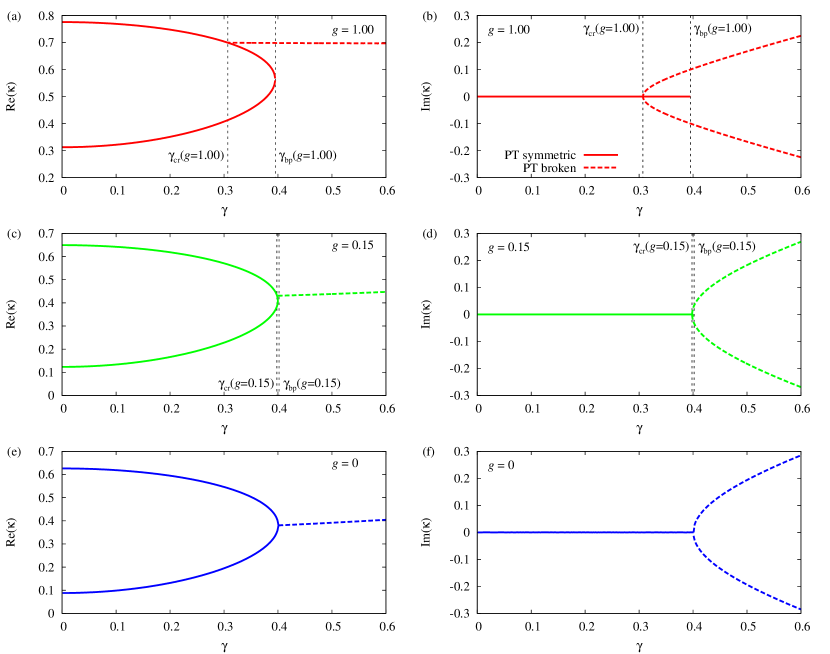
Figure 1: Real parts [(a), (c), (e)] and imaginary parts [(b), (d), (f)] of the eigenvalues $\kappa$ of the full non-linear equation (1) as functions of the loss/gain parameter $\gamma$ for $a=2.2$ and the three values of the non-linearity parameter $g=1.00$ [(a) and (b)], $0.15$ [(c) and (d)] and $0$ [(e) and (f)]. Solid lines denote purely real eigenvalues, dashed lines complex conjugate eigenvalues. For $g\neq 0$ the complex conjugate eigenvalues bifurcate from the ground state branch at $\gamma_{\mathrm{cr}}$ before the branch point $\gamma_{\mathrm{bp}}$ where the two real solutions coalesce. Between $\gamma_{\mathrm{cr}}$ and $\gamma_{\mathrm{bp}}$ the $\mathcal{PT}$-broken and the $\mathcal{PT}$-symmetric branches coexist.

recapitulates the results for the eigenvalues $\kappa$ for different values of the non-linearity parameter $g$. It can be seen that for every value of $g$ a pair of real eigenvalues exists up to some value $\gamma_{\mathrm{bp}}$, where they coalesce at a branch point. Pairs of complex conjugate eigenvalues emerge at critical values $\gamma_{\mathrm{cr}}<\gamma_{\mathrm{bp}}$, where $\gamma_{\mathrm{cr}}$ decreases for increasing $g$. We discuss only examples with $g\geq 0$ in this article, for which the complex conjugate eigenvalues bifurcate from the ground state. Note that the ground state is the upper branch in Figure 1 since the largest value $\kappa$ leads to the lowest energy $E=-\kappa^{2}$. We mention that for $g<0$ the complex eigenvalues branch off from the excited state. For sufficiently large non-linearity these solutions already appear for $\gamma=0$. Thus one has ranges of $\gamma$ where two real and two complex conjugate eigenvalues coexist. The wave functions show that those belonging to the real eigenvalues are themselves $\mathcal{PT}$-symmetric, i.e. they are eigenfunctions of $\mathcal{PT}$, whereas the two states with complex eigenvalues $\kappa$ are not.

Figure 1 reveals that the branching-off of the real eigenvalue changes continuously from the branch for $g=0$. The wave functions, however, show a non-uniform limit as $g$ tends to zero: for every value $g>0$ their asymptotic form is given by $1/\cosh(\kappa x)$, while at $g=0$ it is $\exp(\pm\kappa x)$. The non-uniform behaviour of $g\to 0$ will be addressed in more detail in Section 3.

Pairs of complex conjugate eigenvalues emerge at the branch points only when the non-analytic term $|\psi(x)|^{2}$ in (1) is continued beyond the branch points. This is illustrated in figure 2.

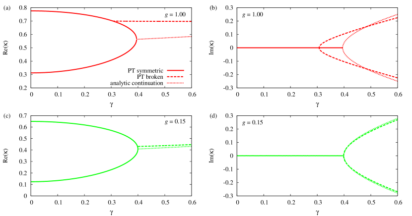
Figure 2: Real parts [(a) and (c)] and imaginary parts [(b) and (d)] of the eigenvalues $\kappa$ for the states appearing at $g=1$ [(a) and (b)] and $g=0.15$ [(c) and (d)]. Using the substitution $|\psi(x)|^{2}\to\psi(x)\psi(-x)$ the analytic continuation beyond the branch point $\gamma_{\mathrm{bp}}$ of the two real $\mathcal{PT}$-symmetric eigenvalue states is obtained.

For the analytic continuation we exploit the $\mathcal{PT}$-symmetry of the wave functions corresponding to the real eigenvalues, i.e. $\psi^{\ast}(x)=\psi(-x)$. Therefore, when approaching the branch point we replace the non-linear term $g|\psi(x)|^{2}$ for the $\mathcal{PT}$-symmetric states by $g\,\psi(x)\psi(-x)$. This function can be continued analytically. We note that in the numerical calculation the additional condition $\int\psi(x)\psi(-x)dx=1$ must be enforced to fix the phase of the non-linearity in the $\mathcal{PT}$ broken regime.

The substitution of $|\psi(x)|^{2}$ by $\psi(x)\psi(-x)$ allowing analytic continuation of the square modulus of $\mathcal{PT}$-symmetric eigenstates shows that the number of solutions does not change at the branch point $\gamma_{\mathrm{bp}}$. Yet, at $\gamma<\gamma_{\mathrm{cr}}<\gamma_{\mathrm{bp}}$ the number of states seem to be less. In fact, the pair of complex eigenvalues bifurcating from the ground state at $\gamma_{\mathrm{cr}}$ seem to come about without real-valued precursors. However, employing a different strategy of complex continuation these precursors and their corresponding eigenstates can indeed also be found.

2.2 Analytic continuation

The procedure [34] is to express all complex quantities by two real-valued functions, either amplitude and phase, or real and imaginary parts. The non-analytic Gross-Pitaevskii equation then decomposes into two coupled real-valued differential equations which can be continued analytically.

We write for the wave function, the double well potential and the eigenvalue $\psi=\psi_{\rm r}+\rmi\psi_{\rm i},\;V=V_{\rm r}+\rmi V_{\rm i}$ and $\kappa=\kappa_{\rm r}+\rmi\kappa_{\rm i}$, respectively. Inserting into the Gross-Pitaevskii equation and sorting the real and imaginary contributions leads to

$$-\psi_{\rm r}^{\prime\prime}+V_{\rm r}\psi_{\rm r}-V_{\rm i}\psi_{\rm i}-g(\psi_{\rm r}^{2}+\psi_{\rm i}^{2})\psi_{\rm r} =\kappa_{\rm r}\psi_{\rm r}-\kappa_{\rm i}\psi_{\rm i}\,,$$ (2a)

$$-\psi_{\rm i}^{\prime\prime}+V_{\rm r}\psi_{\rm i}+V_{\rm i}\psi_{\rm r}-g(\psi_{\rm r}^{2}+\psi_{\rm i}^{2})\psi_{\rm i} =\kappa_{\rm r}\psi_{\rm i}+\kappa_{\rm i}\psi_{\rm r}\,.$$ (2b)

The full analytical extension is implemented by allowing these real and imaginary parts of the wave functions and eigenvalues to become themselves complex:

$$\psi_{\rm r} =\psi_{{\rm r}{\rm r}}+\rmi\psi_{{\rm r}{\rm i}}\,,\quad\psi_{\rm i}=\psi_{\rm i\rm r}+\rmi\psi_{\rm i\rm i}\,,$$ (2ca)

$$\kappa_{\rm r} =\kappa_{\rm r\rm r}+\rmi\kappa_{\rm r\rm i}\,,\quad\kappa_{\rm i}=\kappa_{\rm i\rm r}+\rmi\kappa_{\rm i\rm i}\,.$$ (2cb)

This extension allows for continuing both the $\mathcal{PT}$-symmetric and the $\mathcal{PT}$-broken states beyond the corresponding branch points. When plotting the eigenvalues we recombine the 4 real quantities $\kappa_{\rm r\rm r},\kappa_{\rm r\rm i},\kappa_{\rm i\rm r},\kappa_{\rm i\rm i}$ into the real and imaginary parts of $\kappa$, i. e.

$$\kappa=(\kappa_{\rm r\rm r}-\kappa_{\rm i\rm i})+\rmi(\kappa_{\rm r\rm i}+\kappa_{\rm i\rm r})=\mathrm{Re}(\kappa)+\rmi\,\mathrm{Im}(\kappa)\,.$$ (2cd)

For the value of the non-linearity parameter $g=1$ the results for $\mathrm{Re}(\kappa)$ and $\mathrm{Im}(\kappa)$ are shown in figure 3.

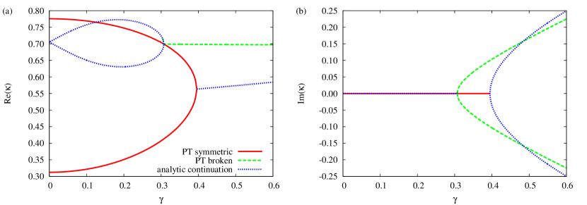
Figure 3: Real parts $\mathrm{Re}(\kappa)$ (a) and imaginary parts $\mathrm{Im}(\kappa)$ (b) of the spectrum after the analytical extension for $g=1$. The red solid and green dashed lines represent the $\mathcal{PT}$-symmetric and $\mathcal{PT}$-broken states already known without any analytic continuation. The new states visible with the full analytic continuation (2ca), (2cb), (2cd) are marked by blue dotted lines. With these continued states the number of states does no longer change with $\gamma$.

For $\gamma\leq\gamma_{\mathrm{cr}}$ there are indeed two new branches of real-valued $\kappa$. They merge at the triple point and give rise to the complex conjugate pair of eigenvalues. Moreover, these two solutions are present even at $\gamma=0$, where they refer to two degenerate eigenvalues.

It is remarkable that the spectra of the two additional states obtained by the analytic continuation become very similar to the spectra of the original $\mathcal{PT}$-symmetric solutions when $g$ is decreased. This is demonstrated in figure 4,

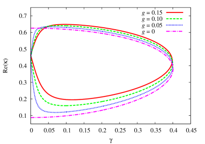
Figure 4: Eigenvalue spectra for $g=0.15$ (red solid lines), $g=0.10$ (green dashed lines), and $g=0.05$ (blue dotted lines). For comparison the spectrum without the non-linear term ($g=0$) is also displayed .

where the spectra shown should be compared with those in figure 1. There is, however, one difference: the two additional solutions are degenerate at $\gamma=0$ for any $g\neq 0$, while the eigenvalues of the two original $\mathcal{PT}$-symmetric states always have different values at this point.

For $g>0$ the wave functions of the analytically continued states shown in figure 4 differ of course from those of the original real eigenvalues where only $\kappa_{\mathrm{rr}}$ features. It is of interest to have a look at these wave functions. They are illustrated for $g=1$ in figure 5

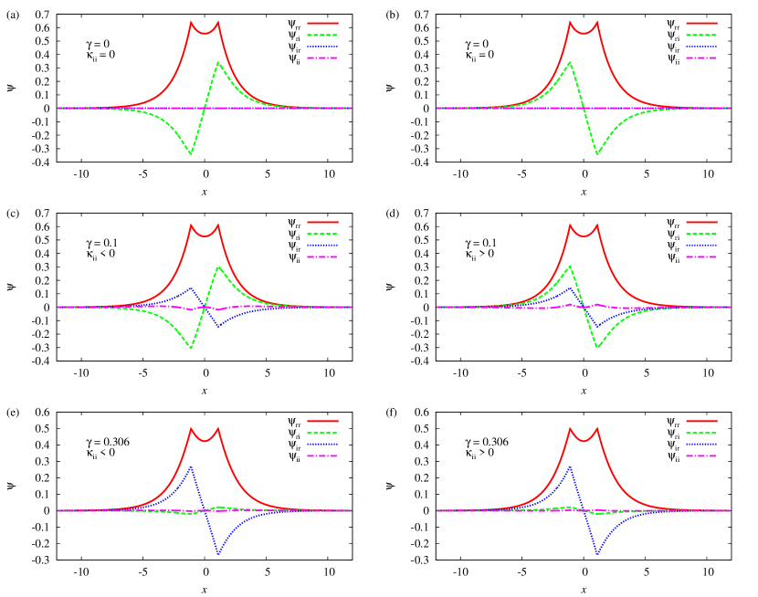
Figure 5: Wave functions of the analytically extended solutions for a few values of $\gamma$ and $g=1$. The right (left) column refers to the lower (upper) branch of the eigenvalues.

for a few values of $0\leq\gamma\leq\gamma_{\mathrm{cr}}$. Note that the functions are eigenfunctions of $\mathcal{PT}$ throughout in that their real parts are symmetric and their imaginary parts antisymmetric. Note further that there is a non-vanishing imaginary part $\psi_{\mathrm{ri}}$ due to the analytic continuation even at $\gamma=0$. At this point the two wave functions are associated with the same energy value as $\kappa_{\rm ii}=0$, i.e. there is a genuine degeneracy. (This in in contrast to the wave functions of the other two energies appearing for $\gamma=0$ (see figure 3)). The imaginary part $\psi_{\mathrm{ri}}$ tends to zero when $\gamma_{\mathrm{cr}}$ is approached while another imaginary part $\psi_{\mathrm{ir}}$ – not due to the analytical continuation – emerges. Eventually, that is at $\gamma_{\mathrm{cr}}$, the two wave functions become equal to themselves and to the third (original) state with which they coalesce at the triple point. From this point onwards the states are found without the complex extension, in fact the parts invoked from the extension vanish. Note also, that the additional real part $\psi_{\rm ii}$ switches on and off at the endpoints of the interval $[0,\gamma_{\mathrm{cr}}$] similar to the behaviour of $\kappa_{\rm ii}$.

2.3 Exceptional point behaviour

As pointed out above the three eigenfunctions are identical at the triple point. Therefore the question arises whether or not the triple point is a third-order exceptional point (denoted by EP3). This is a crucial difference between the nonlinear Gross-Pitaevskii equation [9, 10, 11, 12] and linear $\mathcal{PT}$-symmetric quantum systems, in which the additional triple point does not appear. Exceptional points are isolated singularities of the spectrum in the physical parameter space. We denote by EP2 the point where two states coalesce, i.e. their eigenvalues and their wave functions are identical; similarly, an EP3 denotes the point where three states coalesce. As a function of the parameter the levels and state vectors have a square root singularity at an EP2 and a cubic root singularity at an EP3. As a consequence the eigenvalues and the wave functions are interchanged at an EP2 (up to a possible phase of the latter, see e.g. [35]) when the exceptional point is encircled on a closed contour in parameter space. The three identical wave functions at the triple point indicate an EP3, i.e. a cubic root branch point. For a closed contour around this point a cyclic permutation of all three eigenvalues and eigenfunctions is then observable (see e.g. [36]).

To test numerically the precise character of the exceptional point one parameter must be extended into the complex plane. Confirmation is obtained by encircling the point of coalescence and checking the appropriate change of the eigenvalues and state vectors. Figure 6

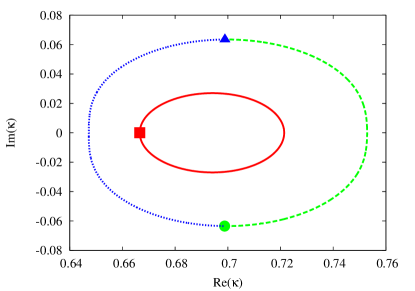
Figure 6: Exceptional point behaviour: circle with complex $\gamma=0.308+0.04\mathrm{e}^{\mathrm{i}\varphi}$, $\varphi=0\dots 2\pi$, for $g=1$, where $\gamma\approx 0.308$ is the triple point. For $\varphi=0$ we have $\gamma=0.312$ and the three states exist without complex continuation. The red square marks the ground state with real $\kappa$. Its trace on the parameter space circle is represented by the red solid line. The two states with positive and negative imaginary parts of the eigenvalues $\kappa$ are represented by the blue triangle (blue dotted line for $\varphi\neq 0$) and the green circle (green dashed line), respectively.

shows the result for a non-linearity of $g=1$ when the triple point at $\gamma_{\mathrm{cr}}\approx 0.308$ is encircled in the complex extended $\gamma$ plane. One clearly sees that only the two complex eigenvalues interchange while the ground state remains unaffected. The same holds for the corresponding eigenfunctions. It thus appears that we deal with an EP2 corresponding to the merging of the two new eigenvalues.

However, when we allow an arbitrarily small asymmetry for the real part of the double well potential by considering $V_{\rm asym}=A\left[\delta(x-a/2)-\delta(x+a/2)\right]$, and encircle now the branch point around $A=0$ in the complex extended $A$ plane, figure 7

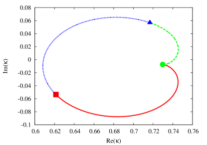
Figure 7: Exceptional point behaviour: circle with complex $A=0.04\mathrm{e}^{\mathrm{i}\varphi}$, $\varphi=0\dots 2\pi$, for $g=1$ and $\gamma=0.308$. The triple point is located exactly at $A=0$. The symbols and lines have the same meaning as in Fig. 6. The circle in the asymmetry parameter clearly reveals the nature of an EP3.

clearly points to an EP3. We stress that any other perturbation would produce the same result: the apparent EP2 which does not involve the third state becomes a true EP3 nesting together all three states as soon as the problem becomes disturbed, no matter of what nature and how small the disturbance may be. This behaviour is similar to that of a study of a simple matrix model by Demange and Graefe [36] where three coalescing eigenvectors can exhibit both the behaviour of second- or third-order exceptional point depending on the choice of parameters. The same behaviour has also been found in the investigation of pitchfork bifurcations occurring in Bose-Einstein condensates with dipolar interaction [37].

To summarise: the numerical solution of the $\mathcal{PT}$-symmetric Gross-Pitaevskii equation (1) brings about spectral properties calling for deeper insight of the physical system. In the following section the precise nature of these spectral singularities will be clarified in analytic terms by means of a matrix model simulating the properties of the non-linear physical system.

3 The Matrix Model

Here we present a simple low-dimensional matrix model that simulates the parameter dependence of the spectrum of the numerical solutions of the Gross-Pitaevskii equation as discussed in the previous section. In particular, the various types of the EPs as found above are of crucial importance: the simulation must reflect the particular types of these spectral singularities.

3.1 General properties

Our starting point is a two-mode model for a $\mathcal{PT}$-symmetric Bose-Einstein condensate [9] that mimics well that of the full Gross-Pitaevskii equation. In the two-mode approximation the $\mathcal{PT}$-symmetric stationary GP-equation assumes the form

$$\pmatrix{-\rmi\gamma+g|\phi_{1}|^{2}&1\cr 1&+\rmi\gamma+g|\phi_{2}|^{2}}\pmatrix{\phi_{1}\cr\phi_{2}}=E\pmatrix{\phi_{1}\cr\phi_{2}}$$ (2ce)

with the normalisation $|\phi_{1}|^{2}+|\phi_{2}|^{2}=1$. The off-diagonal element in the Hamiltonian describes the tunnelling between the two modes, and has been normalised to unity. The analytic extension of the GP-equation in the spirit of Ref. [34] then yields the eigenvalues [9]

$$E_{1} = -\sqrt{1-\gamma^{2}}\,,$$

$$E_{2} = +\sqrt{1-\gamma^{2}}\,,$$

$$E_{3} = g/2-\gamma\sqrt{\frac{1-\gamma^{2}-g^{2}/4}{\gamma^{2}+g^{2}/4}}\,,$$

$$E_{4} = g/2+\gamma\sqrt{\frac{1-\gamma^{2}-g^{2}/4}{\gamma^{2}+g^{2}/4}}\,.$$ (2cf)

Note that here $\gamma_{\rm bp}=1$ and $\gamma_{\rm cr}=\sqrt{1-g^{2}/4}$. In figure 8 such spectra are illustrated for some values of $g$. It is striking how well these eigenvalues quantitatively describe the behaviour of those found numerically from the GP-equation. This perfect simulation includes in particular the spectral singularities and also allows to study the precise behaviour of the non-uniform limit $g\to 0$.

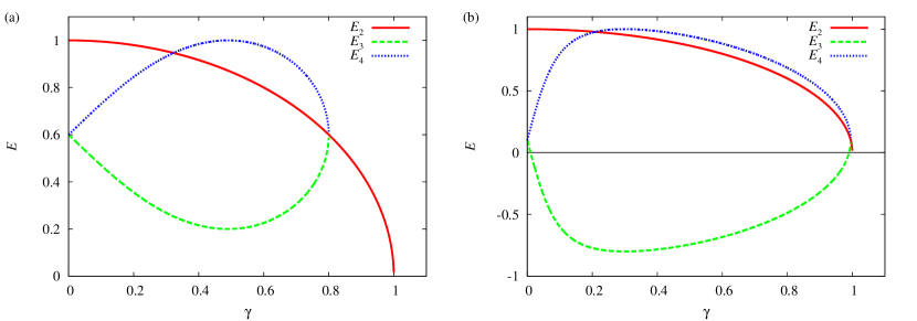
Figure 8: Eigenvalues $E_{2}$, $E_{3}$ and $E_{4}$ from Eq. (2cf) as a function of the non-Hermiticity parameter $\gamma$ for different strengths of the non-linearity, viz. $g=1.2$ (a), $g=0.2$ (b). Note the similarity with the spectra in figure 4.

At the critical point $\gamma=\sqrt{1-g^{2}/4}$ the three eigenvalues $E_{2},E_{3}$ and $E_{4}$ all assume the same value $g/2$. Beyond this point $E_{3}$ and $E_{4}$ become complex; in fact, $E_{3}$ and $E_{4}$ have a square root singularity that appears to have some characteristics of a usual EP. The precise nature, especially its interplay with $E_{2}$, cannot be deduced from the spectrum alone. It is the interaction giving rise to particular wave functions that determines the precise nature of a spectral singularity. As we are interested in the intersection point of the three levels $E_{2},E_{3}$ and $E_{4}$ we restrict ourselves to a three-dimensional matrix model and leave out the level $E_{1}$ altogether as it seems immaterial to our specific interest here.

We seek a three-dimensional matrix, i.e. a model Hamiltonian which produces the spectrum $\{E_{2},E_{3},E_{4}\}$, but in such a way that all levels are fully interacting. This is in contrast to the matrix given in [9] where an interaction between the two branches $E_{1},E_{2}$ and $E_{3},E_{4}$ is not taken into account. In other words, we seek a similarity transformation $s$ such that

$$ham=s\cdot j\cdot s^{-1}$$ (2cg)

where $j$ is diagonal with the levels $\{E_{2},E_{3},E_{4}\}$ in its diagonal and $s$ invokes the interaction between the levels. For our purpose the matrix $s$ must bear all singularities of the eigenvalues, that is of $j$. Moreover, a particular rank drop of $s$ at the critical point $\gamma=\sqrt{1-g^{2}/4}$ indicates as to whether the identical eigenvalues are simply degenerate, or whether there is a coalescence of two or even three eigenstates. In the first case we encounter a usual EP2 and in the second an EP3. Note that $s^{-1}$ does not exist if $s$ does not have full rank whereas $ham$ is still well defined but may no longer be diagonalisable; this is, apart from the branch point behaviour, the algebraic signature of an EP: instead of the diagonal form for $ham$ there exists always the (non-diagonal) Jordan normal form.

A judicious choice fulfilling the requirements is given by

$$s=\pmatrix{1&\sqrt{1-\gamma^{2}}&\sqrt{1-\gamma^{2}}\cr 1&g/2-\gamma\sqrt{\frac{1-\gamma^{2}-g^{2}/4}{\gamma^{2}+g^{2}/4}}&g/2+\gamma\sqrt{\frac{1-\gamma^{2}-g^{2}/4}{\gamma^{2}+g^{2}/4}}\cr 1&(\sqrt{g/2}-\gamma\sqrt{\frac{1-\gamma^{2}-g^{2}/4}{\gamma^{2}+g^{2}/4}})^{2}&(\sqrt{g/2}+\gamma\sqrt{\frac{1-\gamma^{2}-g^{2}/4}{\gamma^{2}+g^{2}/4}})^{2}}.$$ (2ch)

For $\gamma\neq\sqrt{1-g^{2}/4}$ one sees that encircling the critical point in the complex plane swaps the levels $E_{3}$ and $E_{4}$ including their (unnormalised) eigenfunctions listed in $s$ from Eq. (2ch)

$$\pmatrix{\sqrt{1-\gamma^{2}}\cr g/2-\gamma\sqrt{\frac{1-\gamma^{2}-g^{2}/4}{\gamma^{2}+g^{2}/4}}\cr(\sqrt{g/2}-\gamma\sqrt{\frac{1-\gamma^{2}-g^{2}/4}{\gamma^{2}+g^{2}/4}})^{2}}\quad{\rm and}\quad\pmatrix{\sqrt{1-\gamma^{2}}\cr g/2+\gamma\sqrt{\frac{1-\gamma^{2}-g^{2}/4}{\gamma^{2}+g^{2}/4}}\cr(\sqrt{g/2}+\gamma\sqrt{\frac{1-\gamma^{2}-g^{2}/4}{\gamma^{2}+g^{2}/4}})^{2}}$$

being just the characteristic of an EP2. In fact, the square root $\sqrt{1-\gamma^{2}-g^{2}/4}$ simply changes sign when a circle is traced out in the complex $\gamma$-plane around the point $\sqrt{1-g^{2}/4}$ thereby interchanging $E_{3}$ and $E_{4}$ and their corresponding eigenvectors. Note, however, that at the critical point all three eigenvectors also become equal (up to a constant) thus indicating the special nature of this point. In fact, at the critical point the rank drop of $s$ is 2, i.e. rank($s$)=1. At this point $ham$ cannot be diagonalised (recall $s^{-1}$ does not exist), but the Jordan normal form of $ham$ always exists and is given by

$$J[ham]=\pmatrix{g/2&1&0\cr 0&g/2&1\cr 0&0&g/2}.$$ (2ci)

This is the clear algebraic signature of an EP3, where three levels are coalescing. Its analytic counterpart, that is the cubic root behaviour, has been demonstrated in Section 2 by numerical means.

We emphasise that the clear signature of an EP3 as presented above is only available when analytic expressions are at hand. To obtain this result directly by numerical means is virtually impossible. One rather has to resort to the means as presented in the previous section, where the existence of the EP3 is established by invoking an asymmetry and then use closed contours in a suitable complex parameter plane. To elucidate this pattern we discuss in the appendix a three-dimensional matrix demonstrating the underlying mechanism; as our matrix $ham$ is unsuitable for demonstration due to its complicated structure we use a much simplified matrix.

3.2 Behaviour for $g\to 0$

All these statements hold for $g>0$ but care must be taken when $g\to 0$. Recall that the GP-equation has a non-uniform limit for $g\to 0$ as is discussed in Section 2. The same holds for the matrix model when $g\to 0$. As the limiting behaviour is subtle and difficult to obtain numerically, we here give some results obtained in the matrix model. Note in particular how the triple point approaches the branch point where the $\mathcal{PT}$-eigenfunctions meet when $g\to 0$ for the matrix model (figure 8) and $g\to 0$ for the numerical solution (figure 4).

The eigenvalues $E_{3}$ and $E_{4}$ have, for $g>0$, the value $g/2$ at $\gamma=0$. Yet these eigenvalues are $\pm 1$ for $g=0$ and $\gamma=0$. Similarly, the derivative tends to infinity at $\gamma=0$ for $g\to 0$, as can be checked analytically, and is visualized also in figure 8. But it is zero when $g=0$ is taken from the outset. In other words, $E_{4}$ is getting nearer and nearer to $E_{2}$, but at $\gamma=0$ in a non-continuous fashion ($E_{3}$ approaches $-E_{4}$ for $g\to 0$). Note that this behaviour nicely reflects the behaviour of the numerical solutions of the full GP-equation (see figure 4).

At $\gamma=1$ it is the eigenfunctions that show the typical non-uniform behaviour. Note that the eigenvectors as listed in Eq. (2ch) cannot be used in the limits $\gamma\to 1$ and $g\to 0$, irrespective of the order of the limits taken, since $s^{-1}$ does not exist. Rather, the full matrix $ham$ must be considered. If $g=0$, corresponding to switching off the non-linearity in the GP-equation, the eigenvectors of the two positive solutions ($E_{2}=E_{4}=\sqrt{1-\gamma^{2}}$) are given by

$$\pmatrix{0\cr 0\cr 1}\quad{\rm and}\quad\pmatrix{1\cr 1\cr 0}$$

whereas, when the limits are commuted ($\gamma=1$ first and then $g\to 0$) the corresponding eigenvectors are

$$\pmatrix{0\cr 1+\rmi\cr 1}\quad{\rm and}\quad\pmatrix{0\cr 1-\rmi\cr 1}.$$

Recall that $E_{3}$ and $E_{4}$ are complex when $\gamma$ is to the right of the critical point, that is if $\gamma>\sqrt{1-g^{2}/4}$, a condition met for the order of the limits taken. This is reflected here in the complex eigenvectors, even though the eigenvalues are zero in either limit.

A further point of interest is the behaviour of the scalar product taken from the eigenvectors referring to the plain solution for $g=0$ and the eigenvector referring to $g>0$. Of interest is the limit $g\to 0$ of the scalar product. For the eigenvalue $E_{4}=g/2+\gamma\sqrt{\frac{1-\gamma^{2}-g^{2}/4}{\gamma^{2}+g^{2}/4}}$ we obtain for the normalised eigenvectors the scalar product

$$\langle E_{4}^{g>0}|E_{4}^{g=0}\rangle=\frac{g/2+\sqrt{1-\gamma^{2}}+\gamma\sqrt{\frac{1-g^{2}/4-\gamma^{2}}{g^{2}/4+\gamma^{2}}}}{\sqrt{2}\sqrt{1-\gamma^{2}+(\sqrt{g/2}+\gamma\sqrt{\frac{1-\gamma^{2}-g^{2}/4}{\gamma^{2}+g^{2}/4}})^{4}+(g/2+\gamma\sqrt{\frac{1-\gamma^{2}-g^{2}/4}{\gamma^{2}+g^{2}/4}})^{2}}}.$$ (2cj)

We simply list some major facts as they can be easily verified from Eq. (2cj). The scalar product behaves in its limit $g\to 0$ non-uniformly at both ends of the $\gamma$-interval. At $\gamma=0$ Eq. (2cj) assumes the value $(1+g/2)/\sqrt{2+4g^{2}/4}$ whereas the value $\sqrt{2/3}$ is assumed when $g=0$ is set first. At the right end of the $\gamma$-interval the value is unity when $g=0$ while the value is $\sqrt{(1/2+\rmi)}\,(3-\rmi)/5$ when $\gamma=1$ is set before $g\to 0$. We mention that the intricacy of the expansion of $\langle E_{4}^{g>0}|E_{4}^{g=0}\rangle$ in powers of $g$ probably hints to the difficulty in approaching the limit $g\to 0$ numerically using the GP-equation directly. In fact the expansion reads

$$\frac{\sqrt{1-\gamma^{2}}\sqrt{2}}{\sqrt{3-4\gamma^{2}+\gamma^{4}}}-\sqrt{g}\frac{2(\gamma^{2}-1)}{(\gamma^{2}-3)\sqrt{3-4\gamma^{2}+\gamma^{4}}}+\ldots$$

where the $\gamma$-dependent coefficient of $\sqrt{g}$ vanishes for $\gamma=1$; it means that the behaviour of the square root in $g$ will show for $\gamma<1$ but not for $\gamma=1$. In figure 9

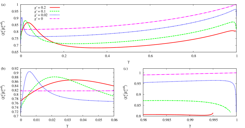
Figure 9: Scalar product of the eigenvector for $g=0$ with the eigenvector for $g^{\prime}\neq 0$ as function of $\gamma$ in the range $0\leq\gamma\leq 1$ (a). The values displayed refer to $g^{\prime}=0.2$ (red solid line), $g^{\prime}=0.1$ (green dashed line), $g^{\prime}=0.02$ (blue dotted line) and $g^{\prime}\to 0$ (purple dashed-dotted line). For better illustration the $\gamma$-axis is stretched at $\gamma=0$ (b) and at $\gamma=1$ (c). All lines are purely real only for $\gamma<\sqrt{1-g^{2}/4}$; it explains the ending for $\gamma<1$ as only pure real values are displayed.

the scalar product is illustrated for a few values of $g$. The non-uniform behaviour at both ends of the $\gamma$-interval is clearly visible. We note that the scalar product assumes the value $\sqrt{2/3}$ at the critical point, independent of $g$.

4 Summary and Conclusions

A number of novel aspects originating from the non-linear term $g|\psi|^{2}$ in the interaction term of the Schrödinger equation are communicated in the present paper. There is the occurrence of two new bound states in the low energy spectrum. Naively, they are seen for $g>0$ only when they emerge as complex solutions from the ground state for $\gamma\geq\gamma_{\rm cr}$ thereby breaking the $\mathcal{PT}$-symmetry of the system. An appropriate complex extension of the GP-equation reveals that two real additional solutions do exist for $\gamma<\gamma_{\rm cr}$ which are in fact eigenfunctions of $\mathcal{PT}$. A further novel result is the triple point at $\gamma=\gamma_{\rm cr}$, in particular the singular spectral behaviour. With a superficial look the singularity appears as a “common” EP2 where the two new solutions turn complex while the ground state from which they emerge seems to be unaffected. However, a more thorough analysis reveals that the three states are nested in an EP3; in fact, for any generic perturbation this result prevails.

While these results are obtained by careful numerical analysis the point $g=0$ being a singular point of the non-linear equation seems to be inaccessible by numerical means. In other words, the limit $g\to 0$ leading to the simpler linear equation is subtle, there is a clear non-uniform behaviour for the spectrum and eigenfunctions. To study this aspect in analytic terms a matrix model simulating quantitatively the spectrum of the GP-equation is presented. While the model elucidates the limit very clearly it also sheds light on the specific behaviour of the triple point: the distinction between the EP2 and EP3 behaviour depending on the specific approach of the singular point becomes evident in analytic terms. The matrix model is designed to be as simple and instructive as possible since our interest is focused upon the explanation of the spectra. An exact quantitative agreement with the numerical results is not intended as it will complicate the analytic discussion.

We believe that these findings are expected to have an impact in experimental work in that specific effects can be detected related to the structure of the model studied. It is well known that EPs have a definite physical significance [35] in a great variety of physical systems. The presence of the triple point has already been established to lead to an instability in the dynamical behaviour [12].

It remains a challenge to detect the signature of the EP3 in a BEC. Whether or not the two additional $\mathcal{PT}$-symmetric states (for $\gamma<\gamma_{\mathrm{cr}}$) merging at $\gamma=\gamma_{\mathrm{cr}}$ into the EP3 have physical significance is, at this stage, an open question. However, it has already been shown that an experimental realisation of a Bose-Einstein condensate in a $\mathcal{PT}$-symmetric double-well setup can be achieved by embedding the double well in a partially tilted multi-well structure [31]. These systems are well accessible with today’s experimental techniques [38, 39, 40]. If they are exposed to loss effects they exhibit resonances, which show as functions of the physical parameters changes of their crossing scenarios, i.e. an effect typical for the presence of exceptional points [41]. It will be interesting to investigate the relation of these exceptional points with those appearing for the balanced gain and loss scenario studied in this article.

As an alternative method for an experimental realisation one may think of introducing spatially separated regions with gain and loss of atoms. Bidirectional couplings between spatially separated condensates have already been realised [42, 43]. Furthermore, electron beams have successfully been used to introduce loss in single sites of optical lattices [44], and an influx of atoms can be achieved by exploiting different electronic states of the atoms to transfer them from a reservoir into one well of a trap [45].

Appendix

The matrix

$$\pmatrix{2&-1&0\cr 2+y&-1&-y\cr-1&0&2}$$

has the spectrum

$$E_{1} = 1$$

$$E_{2} = 1+\sqrt{1-y}$$

$$E_{3} = 1-\sqrt{1-y}.$$

Clearly, and from the structure of the associated eigenfunctions, there is an EP2 at $y=1$. However, when $y=1$ is chosen from the outset the Jordan normal form reads

$$\pmatrix{1&1&0\cr 0&1&1\cr 0&0&1}$$

which clearly indicates an EP3. How to find this by numerical means?

We use a perturbation $\epsilon$

$$\pmatrix{2+\epsilon&-1&0\cr 2+y&-1&-y\cr-1&0&2}.$$

The expansions of the eigenvalues read

$$E_{1} = 1+\frac{2}{1-y}\epsilon+O(\epsilon^{2})$$

$$E_{2} = 1+\sqrt{1-y}+\left(\frac{1+y}{2(1-y)}+\frac{1}{2\sqrt{1-y}}\right)\epsilon+O(\epsilon^{2})$$

$$E_{3} = 1-\sqrt{1-y}+\left(\frac{1+y}{2(1-y)}-\frac{1}{2\sqrt{1-y}}\right)\epsilon+O(\epsilon^{2}).$$

Obviously, the expansion breaks down at the critical point $y=1$. When $y$ is set equal to $1$ in the perturbed matrix, we now see clearly how the eigenvalues sprout from the EP3 in the expected manner. The expansions read now

$$E_{1} = 1-2^{1/3}\exp(2\rmi\pi/3)\epsilon^{1/3}+O(\epsilon^{2/3})$$

$$E_{2} = 1-2^{1/3}\epsilon^{1/3}+O(\epsilon^{2/3})$$

$$E_{3} = 1-2^{1/3}\exp(-2\rmi\pi/3)\epsilon^{1/3}+O(\epsilon^{2/3}).$$

This pattern is basically unchanged for any generic perturbation. It clearly demonstrates the principle underlying in the numerical manifestation of the EP3.

References

References

- [1] C. M. Bender and S. Boettcher. Real spectra in non-Hermitian Hamiltonians having symmetry. Phys. Rev. Lett., 80:5243, 1998.
- [2] N. Moiseyev. Non-Hermitian Quantum Mechanics. Cambridge University Press, Cambridge, 2011.
- [3] S. Diehl, A. Micheli, A. Kantian, B. Kraus, H. P. Büchler, and P. Zoller. Quantum states and phases in driven open quantum systems with cold atoms. Nat. Phys., 4:878–883, 2008.
- [4] D. Witthaut, F. Trimborn, and S. Wimberger. Dissipation induced coherence of a two-mode Bose-Einstein condensate. Phys. Rev. Lett., 101:200402, 2008.
- [5] H. Krauter, C. A. Muschik, K. Jensen, W. Wasilewski, J. M. Petersen, J. I. Cirac, and E. S. Polzik. Entanglement generated by dissipation and steady state entanglement of two macroscopic objects. Phys. Rev. Lett., 107:080503, 2011.
- [6] E. M. Graefe, J. Günther, Korsch H. J., and Niederle A. E. A non-Hermitian symmetric Bose-Hubbard model: eigenvalue rings from unfolding higher-order exceptional points. J. Phys. A, 41:255206, 2008.
- [7] E. M. Graefe, H. J. Korsch, and A. E. Niederle. Mean-field dynamics of a non-Hermitian Bose-Hubbard dimer. Phys. Rev. Lett., 101:150408, 2008.
- [8] E. M. Graefe, H. J. Korsch, and A. E. Niederle. Quantum-classical correspondence for a non-Hermitian Bose-Hubbard dimer. Phys. Rev. A, 82:013629, 2010.
- [9] E. M. Graefe. Stationary states of a symmetric two-mode Bose-Einstein condensate. J. Phys. A, 45:444015, 2012.
- [10] H. Cartarius and G. Wunner. Model of a -symmetric Bose-Einstein condensate in a -function double-well potential. Phys. Rev. A, 86:013612, 2012.
- [11] H. Cartarius, D. Haag, D. Dast, and G. Wunner. Nonlinear Schrödinger equation for a -symmetric delta-function double well. J. Phys. A, 45:444008, 2012.
- [12] D. Dast, D. Haag, H. Cartarius, G. Wunner, R. Eichler, and J. Main. A Bose-Einstein condensate in a symmetric double well. Fortschr. Physik, 61:124–139, 2013.
- [13] H. Ramezani, T. Kottos, R. El-Ganainy, and D. N. Christodoulides. Unidirectional nonlinear -symmetric optical structures. Phys. Rev. A, 82:043803, 2010.
- [14] Z. H. Musslimani, K. G. Makris, R. El-Ganainy, and D. N. Christodoulides. Optical solitons in periodic potentials. Phys. Rev. Lett., 100:30402, 2008.
- [15] F. Kh. Abdullaev, V. V. Konotop, M. Salerno, and A. V. Yulin. Dissipative periodic waves, solitons, and breathers of the nonlinear Schrödinger equation with complex potentials. Phys. Rev. E, 82:056606, 2010.
- [16] Yu. V. Bludov and V. V. Konotop. Nonlinear patterns in Bose-Einstein condensates in dissipative optical lattices. Phys. Rev. A, 81:013625, 2010.
- [17] R. Driben and B. A. Malomed. Stability of solitons in parity-time-symmetric couplers. Opt. Lett., 36:4323–4325, 2011.
- [18] F. Kh. Abdullaev, Y. V. Kartashov, Vladimir V. Konotop, and D. A. Zezyulin. Solitons in -symmetric nonlinear lattices. Phys. Rev. A, 83:41805, 2011.
- [19] Yu. V. Bludov, V. V. Konotop, and B. A. Malomed. Stable dark solitons in -symmetric dual-core waveguides. Phys. Rev. A, 87:013816, Jan 2013.
- [20] A. Guo, G. J. Salamo, D. Duchesne, R. Morandotti, M. Volatier-Ravat, V. Aimez, G. A. Siviloglou, and D. N. Christodoulides. Observation of -symmetry breaking in complex optical potentials. Phys. Rev. Lett., 103:093902, 2009.
- [21] C. E. Rüter, K. G. Makris, R. El-Ganainy, D. N. Christodoulides, M. Segev, and D. Kip. Observation of parity-time symmetry in optics. Nat. Phys., 6:192, 2010.
- [22] Z. H. Musslimani, K. G. Makris, R. El-Ganainy, and D. N. Christodoulides. Analytical solutions to a class of nonlinear Schrödinger equations with -like potentials. J. Phys. A, 41:244019, 2008.
- [23] Th. Mayteevarunyoo, B. A. Malomed, and G. Dong. Spontaneous symmetry breaking in a nonlinear double-well structure. Phys. Rev. A, 78:053601, 2008.
- [24] K. Rapedius and H. J. Korsch. Resonance solutions of the nonlinear Schrödinger equation in an open double-well potential. J. Phys. B, 42:044005, 2009.
- [25] D. Witthaut, K. Rapedius, and H. J. Korsch. The nonlinear Schroedinger equation for the delta-comb potential: quasi-classical chaos and bifurcations of periodic stationary solutions. J. Nonlin. Math. Phys., 16:207–233, 2008.
- [26] V. Jakubský and M. Znojil. An explicitly solvable model of the spontaneous -symmetry breaking. Czech. J. Phys., 55:1113–1116, 2005.
- [27] H. F. Jones. Interface between Hermitian and non-Hermitian Hamiltonians in a model calculation. Phys. Rev. D, 78:065032, 2008.
- [28] A. Mostafazadeh. Delta-function potential with a complex coupling. J. Phys. A, 39:13495, 2006.
- [29] A. Mostafazadeh and H. Mehri-Dehnavi. Spectral singularities, biorthonormal systems and a two-parameter family of complex point interactions. J. Phys. A, 42:125303, 2009.
- [30] H. Mehri-Dehnavi, A. Mostafazadeh, and A. Batal. Application of pseudo-Hermitian quantum mechanics to a complex scattering potential with point interactions. J. Phys. A, 43:145301, 2010.
- [31] M. Kreibich, J. Main, H. Cartarius, and G. Wunner. Hermitian four-well potential as a realization of a -symmetric system. Phys. Rev. A, 87:051601, 2013.
- [32] F. Trimborn, D. Witthaut, and S. Wimberger. Mean-field dynamics of a two-mode Bose-Einstein condensate subject to noise and dissipation. J. Phys. B, 41:171001, 2008.
- [33] D. Witthaut, F. Trimborn, H. Hennig, G. Kordas, T. Geisel, and S. Wimberger. Beyond mean-field dynamics in open Bose-Hubbard chains. Phys. Rev. A, 83:063608, 2011.
- [34] H. Cartarius, J. Main, and G. Wunner. Discovery of exceptional points in the Bose-Einstein condensation of gases with attractive 1/r interaction. Phys. Rev. A, 77:013618, 2008.
- [35] W. D. Heiss. The physics of exceptional points. J. Phys. A, 45:444016, 2012.
- [36] G. Demange and E. M. Graefe. Signatures of three coalescing eigenfunctions. J. Phys. A, 45:025303, 2012.
- [37] R. Gutöhrlein, J. Main, H. Cartarius, and G. Wunner. Bifurcations and exceptional points in dipolar Bose-Einstein condensates. J. Phys. A, in press, Preprint arXiv:1302.5615, 2013.
- [38] T. Salger, C. Geckeler, S. Kling, and M. Weitz. Atomic Landau-Zener tunneling in Fourier-synthesized optical lattices. Phys. Rev. Lett., 99:190405, 2007.
- [39] S. Fölling, S. Trotzky, P. Cheinet, M. Feld, R. Saers, A. Widera, T. Müller, and I. Bloch. Direct observation of second-order atom tunnelling. Nature, 448:1029–1032, 2007.
- [40] K. Henderson, C. Ryu, C. MacCormick, and M. G. Boshier. Experimental demonstration of painting arbitrary and dynamic potentials for Bose-Einstein condensates. New J. Phys., 11:043030, 2009.
- [41] D. Witthaut, E. M. Graefe, S. Wimberger, and H. J. Korsch. Bose-Einstein condensates in accelerated double-periodic optical lattices: Coupling and crossing of resonances. Phys. Rev. A, 75:013617, 2007.
- [42] Y. Shin, G.-B. Jo, M. Saba, T. A. Pasquini, W. Ketterle, and D. E. Pritchard. Optical weak link between two spatially separated Bose-Einstein condensates. Phys. Rev. Lett., 95:170402, 2005.
- [43] R. Gati, M. Albiez, J. Fölling, B. Hemmerling, and M.K. Oberthaler. Realization of a single Josephson junction for Bose-Einstein condensates. Appl. Phys. B, 82:207, 2006.
- [44] T. Gericke, P. Wurtz, D. Reitz, T. Langen, and H. Ott. High-resolution scanning electron microscopy of an ultracold quantum gas. Nature Phys., 4:949–953, 2008.
- [45] N. P. Robins, C. Figl, M. Jeppesen, G. R. Dennis, and J. D. Close. A pumped atom laser. Nature Phys., 4:731–736, 2008.