Second-Order Non-Stationary Online Learning
for Regression

Abstract

The goal of a learner, in standard online learning, is to have the cumulative loss not much larger compared with the best-performing function from some fixed class. Numerous algorithms were shown to have this gap arbitrarily close to zero, compared with the best function that is chosen off-line. Nevertheless, many real-world applications, such as adaptive filtering, are non-stationary in nature, and the best prediction function may drift over time. We introduce two novel algorithms for online regression, designed to work well in non-stationary environment. Our first algorithm performs adaptive resets to forget the history, while the second is last-step min-max optimal in context of a drift. We analyze both algorithms in the worst-case regret framework and show that they maintain an average loss close to that of the best slowly changing sequence of linear functions, as long as the cumulative drift is sublinear. In addition, in the stationary case, when no drift occurs, our algorithms suffer logarithmic regret, as for previous algorithms. Our bounds improve over the existing ones, and simulations demonstrate the usefulness of these algorithms compared with other state-of-the-art approaches.

I Introduction

We consider the classical problem of online learning for regression. On each iteration, an algorithm receives a new instance (for example, input from an array of antennas) and outputs a prediction of a real value (for example distance to the source). The correct value is then revealed, and the algorithm suffers a loss based on both its prediction and the correct output value.

In the past half a century many algorithms were proposed (see e.g. a comprehensive book [9]) for this problem, some of which are able to achieve an average loss arbitrarily close to that of the best function in retrospect. Furthermore, such guarantees hold even if the input and output pairs are chosen in a fully adversarial manner with no distributional assumptions. Many of these algorithms exploit first-order information (e.g. gradients).

Recently there is an increased amount of interest in algorithms that exploit second order information. For example the second order perceptron algorithm [8], confidence-weighted learning [13, 11], adaptive regularization of weights (AROW) [12], all designed for classification; and AdaGrad [14] and FTPRL [28] for general loss functions.

Despite the extensive and impressive guarantees that can be made for algorithms in such settings, competing with the best fixed function is not always good enough. In many real-world applications, the true target function is not fixed, but is slowly changing over time. Consider a filter designed to cancel echoes in a hall. Over time, people enter and leave the hall, furniture are being moved, microphones are replaced and so on. When this drift occurs, the predictor itself must also change in order to remain relevant.

With such properties in mind, we develop new learning algorithms, based on second-order quantities, designed to work with target drift. The goal of an algorithm is to maintain an average loss close to that of the best slowly changing sequence of functions, rather than compete well with a single function. We focus on problems for which this sequence consists only of linear functions. Most previous algorithms (e.g. [27, 1, 23, 26]) designed for this problem are based on first-order information, such as gradient descent, with additional control on the norm of the weight-vector used for prediction [26] or the number of inputs used to define it [6].

In Sec. II we review three second-order learning algorithms: the recursive least squares (RLS) [22] algorithm, the Aggregating Algorithm for regression (AAR) ([21, 36]), which can be shown to be derived based on a last-step min-max approach [16], and the AROWR algorithm [35] which is a modification of the AROW algorithm [12] for regression. All three algorithms obtain logarithmic regret in the stationary setting, although derived using different approaches, and they are not equivalent in general. In Sec. III we formally present the non-stationary setting both in terms of algorithms and in terms of theoretical analysis.

For the RLS algorithm, a variant called CR-RLS ([31, 20, 10]) for the non-stationary setting was described, yet not analyzed, before. In Sec. IV we present two algorithms for the non-stationary setting, that build on the other two algorithms. Specifically, in Sec. IV-A we extend the AROWR algorithm for the non-stationary setting, yielding an algorithm called ARCOR for adaptive regularization with covariance reset. Similar to CR-RLS, ARCOR performs a step called covariance-reset, which resets the second-order information from time-to-time, yet it is done based on the properties of this covariance-like matrix, and not based on the number of examples observed, as in CR-RLS.

In Sec. IV-B we derive different algorithm based on the last-step min-max approach proposed by Forster [16] and later used [34] for online density estimation. On each iteration the algorithm makes the optimal min-max prediction with respect to the regret, assuming it is the last iteration. Yet, unlike previous work [16], it is optimal when a drift is allowed. As opposed to the derivation of the last-step min-max predictor for a fixed vector, the resulting optimization problem is not straightforward to solve. We develop a dynamic program (a recursion) to solve this problem, which allows to compute the optimal last-step min-max predictor. We call this algorithm LASER for last step adaptive regressor algorithm. We conclude the algorithmic part in Sec. IV-C in which we compare all non-stationary algorithms head-to-head highlighting their similarities and differences. Additionally, after describing the details of our algorithms, we provide in Sec. V a comprehensive review of previous work, that puts our contribution in perspective. Both algorithms reduce to their stationary counterparts when no drift occurs.

We then move to Sec. VI which summarizes our next contribution stating and proving regret bounds for both algorithms. We analyse both algorithms in the worst-case regret-setting and show that as long as the amount of average-drift is sublinear, the average-loss of both algorithms will converge to the average-loss of the best sequence of functions. Specifically, we show in Sec. VI-A that the cumulative loss of ARCOR after observing $T$ examples, denoted by $L_{T}(\textrm{ARCOR})$, is upper bounded by the cumulative loss of any sequence of weight-vectors $\{{\boldsymbol{u}}_{t}\}$, denoted by $L_{T}(\{{\boldsymbol{u}}_{t}\})$, plus an additional term ${\mathcal{O}}\left({T^{1/2}\left({V(\{{\boldsymbol{u}}_{t}\})}\right)^{1/2}\log T}\right)$ where $V(\{{\boldsymbol{u}}_{t}\})$ measures the differences (or variance) between consecutive weight-vectors of the sequence $\{{\boldsymbol{u}}_{t}\}$. Later, we show in Sec. VI-B a similar bound for the loss of LASER, denoted by $L_{T}(\textrm{LASER})$, for which the second term is ${\mathcal{O}}\left({T^{2/3}\left({V(\{{\boldsymbol{u}}_{t}\})}\right)^{1/3}}\right)$. We emphasize that in both bounds the measure $V(\{{\boldsymbol{u}}_{t}\})$ of differences between consecutive weight-vectors is not defined in the same way, and thus, the bounds are not comparable in general.

In Sec. VII we report results of simulations designed to highlight the properties of both algorithms, as well as the commonalities and differences between them. We conclude in Sec. VIII and most of the technical proofs appear in the appendix.

The ARCOR algorithm was presented in a shorter publication [35], as well with its analysis and some of its details. The LASER algorithm and its analysis was also presented in a shorter version [30]. The contribution of this submission is three-fold. First, we provide head-to-head comparison of three second-order algorithms for the stationary case. Second, we fill the gap of second-order algorithms for the non-stationary case. Specifically, we add to the CR-RLS (which extends RLS) and design second-order algorithms for the non-stationary case and analyze them, building both on AROWR and AAR. Our algorithms are derived from different principles from each other, which is reflected in our analysis. Finally, we provide empirical evidence showing that under various conditions different algorithm performs the best.

Some notation we use throughout the paper: For a symmetric matrix $\Sigma$ we denote its j$th$ eigenvalue by $\lambda_{j}(\Sigma)$. Similarly we denote its smallest eigenvalue by $\lambda_{min}(\Sigma)=\min_{j}\lambda_{j}(\Sigma)$, and its largest eigenvalue by $\lambda_{max}(\Sigma)=\max_{j}\lambda_{j}(\Sigma)$. For a vector ${\boldsymbol{u}}\in\mathbb{R}^{d}$, we denote by $\|{\boldsymbol{u}}\|$ the $\ell_{2}$-norm of the vector. Finally, for $y>0$ we define $clip(x,y)={\rm sign}(x)\min\{|x|,y\}$.

II Stationery Online Learning

We focus on the regression task evaluated with the squared loss. Our algorithms are designed for the online setting and work in iterations (or rounds). On each round an online algorithm receives an input-vector ${\boldsymbol{x}}_{t}\in\mathbb{R}^{d}$ and predicts a real value $\hat{y}_{t}\in\mathbb{R}$. Then the algorithm receives a target label $y_{t}\in\mathbb{R}$ associated with ${\boldsymbol{x}}_{t}$, and uses it to update its prediction rule, and proceeds to the next round.

At each iteration, the performance of the algorithm is evaluated using the squared loss, $\ell_{t}(\textrm{alg})=\ell\left({y_{t},\hat{y}_{t}}\right)=\left({\hat{y}_{t}-y_{t}}\right)^{2}$. The cumulative loss suffered by the algorithm over $T$ iterations is, $L_{T}(\textrm{alg})=\sum_{t=1}^{T}\ell_{t}(\textrm{alg}).$

The goal of the algorithm is to have low cumulative loss compared to predictors from some class. A large body of work, which we adopt as well, is focused on linear prediction functions of the form $f({\boldsymbol{x}})={{\boldsymbol{x}}}^{\top}{\boldsymbol{u}}$ where ${\boldsymbol{u}}\in\mathbb{R}^{d}$ is some weight-vector. We denote by $\ell_{t}({\boldsymbol{u}})=\left({{{\boldsymbol{x}}}^{\top}_{t}{\boldsymbol{u}}-y_{t}}\right)^{2}$ the instantaneous loss of a weight-vector ${\boldsymbol{u}}$. The cumulative loss suffered by a fixed weight-vector ${\boldsymbol{u}}$ is, $L_{T}({\boldsymbol{u}})=\sum_{t}^{T}\ell_{t}({\boldsymbol{u}})$.

The goal of the learning algorithm is to suffer low loss compared with the best linear function. Formally we define the regret of an algorithm to be

$${R}(T)=L_{T}(\textrm{alg})-\inf_{\boldsymbol{u}}L_{T}({\boldsymbol{u}})~{}.$$ (1)

The goal of an algorithm is to have ${R}(T)=o(T)$, such that the average loss will converge to the average loss of the best linear function ${\boldsymbol{u}}$.

Numerous algorithms were developed for this problem, see a comprehensive review in the book of Cesa-Bianchi and Lugosi [9]. Among these, a few second-order online algorithms for regression were proposed in recent years, which we summarize in Table I. One approach for online learning is to reduce the problem into consecutive batch problems, and specifically use all previous examples to generate a classifier, which is used to predict current example. Recursive least squares (RLS) [22] approach, for example, sets a weight-vector to be the solution of the following optimization problem,

$${\boldsymbol{w}}_{t}=\arg\min_{\boldsymbol{w}}\left({\sum_{i=1}^{t}r^{t-i}\left({y_{i}-{\boldsymbol{w}}\cdot{\boldsymbol{x}}_{i}}\right)^{2}}\right)$$

Since the last problem grows with time, the well known recursive least squares (RLS) [22] algorithm was developed to generate a solution recursively. The RLS algorithm maintains both a vector ${\boldsymbol{w}}_{t}$ and a positive semi-definite (PSD) matrix $\Sigma_{t}$. On each iteration, after making a prediction $\hat{y}_{t}={{\boldsymbol{x}}}^{\top}_{t}{\boldsymbol{w}}_{t-1}$, the algorithm receives the true label $y_{t}$ and updates,

$${\boldsymbol{w}}_{t} ={\boldsymbol{w}}_{t-1}+\frac{(y_{t}-{{\boldsymbol{x}}}^{\top}_{t}{\boldsymbol{w}}_{t-1})\Sigma_{t-1}{\boldsymbol{x}}_{t}}{r+{{\boldsymbol{x}}}^{\top}_{t}\Sigma_{t-1}{\boldsymbol{x}}_{t}}$$ (2)

$${\Sigma}_{t}^{-1} =r\Sigma_{t-1}^{-1}+{\boldsymbol{x}}_{t}{{\boldsymbol{x}}}^{\top}_{t}~{}.$$ (3)

The update of the prediction vector ${\boldsymbol{w}}_{t}$ is additive, with vector $\Sigma_{t-1}{\boldsymbol{x}}_{t}$ scaled by the error $(y_{t}-{{\boldsymbol{x}}}^{\top}_{t}{\boldsymbol{w}}_{t-1})$ over the norm of the input measured using the norm defined by the matrix ${{\boldsymbol{x}}}^{\top}_{t}\Sigma_{t-1}{\boldsymbol{x}}_{t}$. The algorithm is summarized in the right column of Table I.

The Aggregating Algorithm for regression (AAR) [21, 36], summarized in the middle column of Table I, was introduced by Vovk and it is similar to the RLS algorithm, except it shrinks its predictions. The AAR algorithm was shown to be last-step min-max optimal by Forster [16]. Given a new input ${\boldsymbol{x}}_{T}$ the algorithm predicts $\hat{y}_{T}$ which is the minimizer of the following problem,

$$\arg\min_{\hat{y}_{T}}\max_{y_{T}}\left[{\sum_{t=1}^{T}(y_{t}-\hat{y}_{t})^{2}-\inf_{{\boldsymbol{u}}}\left({b\left\|{\boldsymbol{u}}\right\|^{2}+L_{T}({\boldsymbol{u}})}\right)}\right].\!\!\!$$ (4)

Forster proposed also a simpler analysis with the same regret bound.

Finally, the AROWR algorithm [35] is a modification of the AROW algorithm [12] for regression. In a nutshell, the AROW algorithm maintains a Gaussian distribution parameterized by a mean ${\boldsymbol{w}}_{t}\in\mathbb{R}^{d}$ and a full covariance matrix $\Sigma_{t}\in\mathbb{R}^{d\times d}$. Intuitively, the mean ${\boldsymbol{w}}_{t}$ represents a current linear function, while the covariance matrix $\Sigma_{t}$ captures the uncertainty in the linear function ${\boldsymbol{w}}_{t}$. Given a new example $({\boldsymbol{x}}_{t},y_{t})$ the algorithm uses its current mean to make a prediction $\hat{y}_{t}={{\boldsymbol{x}}}^{\top}_{t}{\boldsymbol{w}}_{t-1}$. AROWR then sets the new distribution to be the solution of the following optimization problem,

$$\arg\min_{{\boldsymbol{w}},\Sigma}~{} {\textrm{D}_{\textrm{KL}}}\left({{\mathcal{N}}\left({{\boldsymbol{w}},\Sigma}\right)\,\|\,{\mathcal{N}}\left({{\boldsymbol{w}}_{t-1},\Sigma_{t-1}}\right)}\right)$$

$$+\frac{1}{2r}\left({y_{t}-{{\boldsymbol{w}}}^{\top}{\boldsymbol{x}}_{t}}\right)^{2}+\frac{1}{2r}\left({{{\boldsymbol{x}}}^{\top}_{t}\Sigma{\boldsymbol{x}}_{t}}\right)$$ (5)

This optimization problem is similar to the one of AROW [12] for classification, except we use the square loss rather than squared-hinge loss used in AROW. Intuitively, the optimization problem trades off between three requirements. The first term forces the parameters not to change much per example, as the entire learning history is encapsulated within them. The second term requires that the new vector ${\boldsymbol{w}}_{t}$ should perform well on the current instance, and finally, the third term reflects the fact that the uncertainty about the parameters reduces as we observe the current example ${\boldsymbol{x}}_{t}$.

The weight vector solving this optimization problem (details given by Vaits and Crammer [35]) is given by,

$${\boldsymbol{w}}_{t} ={\boldsymbol{w}}_{t-1}+\left({\frac{y_{t}-{\boldsymbol{w}}_{t-1}\cdot{\boldsymbol{x}}_{t}}{r+{{\boldsymbol{x}}}^{\top}_{t}\Sigma_{t-1}{\boldsymbol{x}}_{t}}}\right)\Sigma_{t-1}{\boldsymbol{x}}_{t}~{},$$ (6)

and the optimal covariance matrix is,

$$\Sigma_{t}^{-1}=\Sigma_{t-1}^{-1}+\frac{1}{r}{\boldsymbol{x}}_{t}{{\boldsymbol{x}}}^{\top}_{t}~{}.$$ (7)

The algorithm is summarized in the left column of Table I. Comparing AROW to RLS we observe that while the update of the weights of (6) is equivalent to the update of RLS in (2), the update of the matrix (3) for RLS is not equivalent to (7), as in the former case the matrix goes via a multiplicative update as well as additive, while in (7) the update is only additive. The two updates are equivalent only by setting $r=1$. Moving to AAR, we note that the update rules for ${\boldsymbol{w}}_{t}$ and $\Sigma_{t}$ in AROWR and AAR are the same if we define $\Sigma_{t}^{AAR}=\Sigma_{t}^{AROWR}/r$, but AROWR does not shrink its predictions as AAR. Thus all three algorithms are not equivalent, although very similar.

III Non-Stationary Online Learning

All previous algorithms assume both by design and analysis that the data is stationary. The analysis of all algorithms compares their performance to that of a single fixed weight vector ${\boldsymbol{u}}$, and all suffer regret that is logarithmic is $T$.

We use an extended notion of evaluation, comparing our algorithms to a sequence of functions. We define the loss suffered by such a sequence to be,

$$L_{T}({\boldsymbol{u}}_{1},\ldots,{\boldsymbol{u}}_{T})=L_{T}(\{{\boldsymbol{u}}_{t}\})=\sum_{t}^{T}\ell_{t}({\boldsymbol{u}}_{t})~{},$$

and the regret is then defined to be,

$${R}(T)=L_{T}(\textrm{alg})-\inf_{{\boldsymbol{u}}_{1},\ldots,{\boldsymbol{u}}_{T}}L_{T}(\{{\boldsymbol{u}}_{t}\})~{}.$$ (8)

We focus on algorithms that are able to compete against sequences of weight-vectors, $({\boldsymbol{u}}_{1},\ldots,{\boldsymbol{u}}_{T})\in\mathbb{R}^{d}\times\dots\times\mathbb{R}^{d}$, where ${\boldsymbol{u}}_{t}$ is used to make a prediction for the t$th$ example $({\boldsymbol{x}}_{t},y_{t})$.

Clearly, with no restriction over the set $\{{\boldsymbol{u}}_{t}\}$ the right term of the regret can easily be zero by setting, ${\boldsymbol{u}}_{t}={\boldsymbol{x}}_{t}(y_{t}/\left\|{{\boldsymbol{x}}_{t}}\right\|^{2})$, which implies $\ell_{t}({\boldsymbol{u}}_{t})=0$ for all $t$. Thus, in the analysis below we will make use of the total drift of the weight-vectors defined to be,

$$V^{(P)}=V^{(P)}_{T}(\{{\boldsymbol{u}}_{t}\})=\sum_{t=1}^{T-1}\|{\boldsymbol{u}}_{t}-{\boldsymbol{u}}_{t+1}\|^{P}~{},$$

where $P\in\{1,2\}$.

For all three algorithms, as was also observed previously in the context of CW [13], AROW [12], AdaGrad [14] and FTPRL [28], the matrix $\Sigma$ can be interpreted as adaptive learning rate. As these algorithms process more examples, that is larger values of $t$, the eigenvalues of the matrix ${\Sigma}_{t}^{-1}$ increase, and the eigenvalues of the matrix ${\Sigma}_{t}$ decrease, and we get that the rate of updates is getting smaller, since the additive term $\Sigma_{t-1}{\boldsymbol{x}}_{t}$ is getting smaller. As a consequence the algorithms will gradually stop updating using current instances which lie in the subspace of examples that were previously observed numerous times. This property leads to a very fast convergence in the stationary case. However, when we allow these algorithms to be compared with a sequence of weight-vectors, each applied to a different input example, or equivalently, there is a drift or shift of a good prediction vector, these algorithms will perform poorly, as they will converge and not be able to adapt to the non-stationarity nature of the data.

This phenomena motivated the proposal of the CR-RLS algorithm ([31, 20, 10]), which re-sets the covariance matrix every fixed number of input examples, causing the algorithm not to converge or get stuck. The pseudo-code of CR-RLS algorithm is given in the right column of Table II. The only difference of CR-RLS from RLS is that after updating the matrix $\Sigma_{t}$, the algorithm checks whether $T_{0}$ (a predefined natural number) examples were observed since the last restart, and if this is the case, it sets the matrix to be the identity matrix. Clearly, if $T_{0}=\infty$ the CR-RLS algorithm is reduced to the RLS algorithm.

TABLE I: Algorithms for stationary setting

		AROWR	AAR	RLS
Parameters		$0<r$	$0<b$	$0<r\leq 1$
Initialize		${\boldsymbol{w}}_{0}=0~{},~{}\Sigma_{0}=I$	${\boldsymbol{w}}_{0}=0~{},~{}\Sigma_{0}=b^{-1}I$	${\boldsymbol{w}}_{0}=0~{},~{}\Sigma_{0}=I$
		Receive an instance ${\boldsymbol{x}}_{t}$
For	Output	$$\hat{y}_{t}={{\boldsymbol{x}}}^{\top}_{t}{\boldsymbol{w}}_{t-1}$$	$$\hat{y}_{t}=\frac{{{\boldsymbol{x}}}^{\top}_{t}{\boldsymbol{w}}_{t-1}}{1+{{\boldsymbol{x}}}^{\top}_{t}\Sigma_{t-1}{\boldsymbol{x}}_{t}}$$	$$\hat{y}_{t}={{\boldsymbol{x}}}^{\top}_{t}{\boldsymbol{w}}_{t-1}$$
$t=1...T$	prediction
		Receive a correct label $y_{t}$
	Update $\Sigma_{t}$:	$$\Sigma_{t}^{-1}=\Sigma_{t-1}^{-1}+\frac{1}{r}{\boldsymbol{x}}_{t}{{\boldsymbol{x}}}^{\top}_{t}$$	$$\Sigma_{t}^{-1}=\Sigma_{t-1}^{-1}+{\boldsymbol{x}}_{t}{{\boldsymbol{x}}}^{\top}_{t}$$	$$\Sigma_{t}^{-1}=r\Sigma_{t-1}^{-1}+{\boldsymbol{x}}_{t}{{\boldsymbol{x}}}^{\top}_{t}$$
	Update ${\boldsymbol{w}}_{t}$:	$$\begin{array}[]{ll}{\boldsymbol{w}}_{t}&\!\!\!\!={\boldsymbol{w}}_{t-1}\\ &\!\!\!\!+\frac{(y_{t}-{{\boldsymbol{x}}}^{\top}_{t}{\boldsymbol{w}}_{t-1})\Sigma_{t-1}{\boldsymbol{x}}_{t}}{r+{{\boldsymbol{x}}}^{\top}_{t}\Sigma_{t-1}{\boldsymbol{x}}_{t}}\\ {}\\ \end{array}$$	$$\!\!\!\!\!\!\begin{array}[]{ll}{\boldsymbol{w}}_{t}&\!\!\!\!\!={\boldsymbol{w}}_{t-1}\\ &\!\!\!\!\!+\frac{(y_{t}-{{\boldsymbol{x}}}^{\top}_{t}{\boldsymbol{w}}_{t-1})\Sigma_{t-1}{\boldsymbol{x}}_{t}}{1+{{\boldsymbol{x}}}^{\top}_{t}\Sigma_{t-1}{\boldsymbol{x}}_{t}}\end{array}$$	$$\begin{array}[]{ll}{\boldsymbol{w}}_{t}&\!\!\!\!={\boldsymbol{w}}_{t-1}\\ &\!\!\!\!+\frac{(y_{t}-{{\boldsymbol{x}}}^{\top}_{t}{\boldsymbol{w}}_{t-1})\Sigma_{t-1}{\boldsymbol{x}}_{t}}{r+{{\boldsymbol{x}}}^{\top}_{t}\Sigma_{t-1}{\boldsymbol{x}}_{t}}\end{array}$$
Output		${\boldsymbol{w}}_{T}\ ,\ \Sigma_{T}$	${\boldsymbol{w}}_{T}\ ,\ \Sigma_{T}$	${\boldsymbol{w}}_{T}\ ,\ \Sigma_{T}$
Extension to non-stationary setting		ARCOR Sec. IV-A below	LASER Sec. IV-B      below	CR-RLS [31, 20, 10]
Analysis		yes, Sec. VI-A           below	yes, Sec. VI-B           below	No

IV Algorithms for Non-Stationary Regression

In this work we fill the gap and propose extension to non-stationary setting for the two other algorithms in Table I. Similar to CR-RLS, both algorithms modify the matrix $\Sigma_{t}$ to prevent its eigen-values to shrink to zero. The first algorithm, described in Sec. IV-A, extends AROWR to the non-stationary setting and is similar in spirit to CR-RLS, yet the restart operations it performs depend on the spectral properties of the covariance matrix, rather than the time index $t$. Additionally, this algorithm performs a projection of the weight vector into a predefined ball. Similar technique was used in first order algorithms by Herbster and Warmuth [23], and Kivinen and Warmuth [25]. Both steps are motivated both from the design and analysis of AROWR. Its design is composed of solving small optimization problems defined in (5), one per input example. The non-stationary version performs explicit corrections to its update, in order to prevent from the covariance matrix to shrink to zero, and the weight-vector to grow too fast.

The second algorithm described in Sec. IV-B is based on a last-step min-max prediction principle and objective, where we replace $L_{T}({\boldsymbol{u}})$ in (4) with $L_{T}(\{{\boldsymbol{u}}_{t}\})$ and some additional modifications preventing the solution being degenerate. Here the algorithmic modifications from the original AAR algorithm are implicit and are due to the modifications of the objective. The resulting algorithm smoothly interpolates the covariance matrix with a unit matrix.

IV-A ARCOR: Adaptive regularization of weights for Regression with COvariance Reset

Our first algorithm is based on the AROWR. We propose two modifications to (6) and (7), which in combination overcome the problem that the algorithm’s learning rate gradually goes to zero. The modified algorithm operates on segments of the input sequence. In each segment indexed by $i$, the algorithm checks whether the lowest eigenvalue of $\Sigma_{t}$ is greater than a given lower bound $\Lambda_{i}$. Once the lowest eigenvalue of $\Sigma_{t}$ is smaller than $\Lambda_{i}$ the algorithm resets $\Sigma_{t}=I$ and updates the value of the lower bound $\Lambda_{i+1}$. Formally, the algorithm uses the update (7) to compute an intermediate candidate for $\Sigma_{t}$, denoted by

$$\tilde{\Sigma}_{t}=\left({\Sigma_{t-1}^{-1}+\frac{1}{r}{\boldsymbol{x}}_{t}{{\boldsymbol{x}}}^{\top}_{t}}\right)^{-1}.$$ (9)

If indeed $\tilde{\Sigma}_{t}\succeq\Lambda_{i}I$ then it sets $\Sigma_{t}=\tilde{\Sigma}_{t}$, otherwise it sets $\Sigma_{t}=I$ and the segment index is increased by $1$.

Additionally, before our modification, the norm of the weight vector ${\boldsymbol{w}}_{t}$ did not increase much as the “effective” learning rate (the matrix $\Sigma_{t}$) went to zero. After our update, as the learning rate is effectively bounded from below, the norm of ${\boldsymbol{w}}_{t}$ may increase too fast, which in turn will cause a low update-rate in non-stationarity inputs.

We thus employ additional modification which is exploited by the analysis. After updating the mean ${\boldsymbol{w}}_{t}$ as in (6)

$$\tilde{{\boldsymbol{w}}}_{t} ={\boldsymbol{w}}_{t-1}+\frac{(y_{t}-{{\boldsymbol{x}}}^{\top}_{t}{\boldsymbol{w}}_{t-1})\Sigma_{t-1}{\boldsymbol{x}}_{t}}{r+{{\boldsymbol{x}}}^{\top}_{t}\Sigma_{t-1}{\boldsymbol{x}}_{t}},$$ (10)

we project it into a ball $B$ around the origin of radius $R_{B}$ using a Mahalanobis distance. Formally, we define the function $\textrm{proj}(\tilde{{\boldsymbol{w}}},\Sigma,R_{B})$ to be the solution of the following optimization problem,

$$\arg\min_{\|{\boldsymbol{w}}\|\leq R_{B}}\frac{1}{2}\left({{\boldsymbol{w}}-\tilde{{\boldsymbol{w}}}}\right)^{\top}\Sigma^{-1}\left({{\boldsymbol{w}}-\tilde{{\boldsymbol{w}}}}\right)$$

We write the Lagrangian,

$${\mathcal{L}}=\frac{1}{2}\left({{\boldsymbol{w}}-\tilde{{\boldsymbol{w}}}}\right)^{\top}\Sigma^{-1}\left({{\boldsymbol{w}}-\tilde{{\boldsymbol{w}}}}\right)+\alpha\left({\frac{1}{2}\|{\boldsymbol{w}}\|^{2}-\frac{1}{2}R_{B}^{2}}\right)~{}.$$

Setting the gradient with respect to ${\boldsymbol{w}}$ to zero we get, $\Sigma^{-1}\left({{\boldsymbol{w}}-\tilde{{\boldsymbol{w}}}}\right)+\alpha{\boldsymbol{w}}=0$. Solving for ${\boldsymbol{w}}$ we get

$${\boldsymbol{w}}=\left({\alpha I+\Sigma^{-1}}\right)^{-1}\Sigma^{-1}\tilde{{\boldsymbol{w}}}=\left({I+\alpha\Sigma}\right)^{-1}\tilde{{\boldsymbol{w}}}~{}.$$

From KKT conditions we get that if $\|\tilde{{\boldsymbol{w}}}\|\leq R_{B}$ then $\alpha=0$ and ${\boldsymbol{w}}=\tilde{{\boldsymbol{w}}}$. Otherwise, $\alpha$ is the unique positive scalar that satisfies $\|\left({I+\alpha\Sigma}\right)^{-1}\tilde{{\boldsymbol{w}}}\|=R_{B}$. The value of $\alpha$ can be found using binary search and eigen-decomposition of the matrix $\Sigma$. We write explicitly $\Sigma=V\Lambda V^{\top}$ for a diagonal matrix $\Lambda$. By denoting ${\boldsymbol{u}}=V^{\top}\tilde{{\boldsymbol{w}}}$ we rewrite the last equation, $\|\left({I+\alpha\Lambda}\right)^{-1}{\boldsymbol{u}}\|=R_{B}$. We thus wish to find $\alpha$ such that $\sum_{j}^{d}\frac{u_{j}^{2}}{(1+\alpha\Lambda_{j,j})^{2}}=R_{B}^{2}$. It can be done using a binary search for $\alpha\in[0,a]$ where $a=(\|{\boldsymbol{u}}\|/R_{B}-1)/\lambda_{\min}(\Lambda)$. To summarize, the projection step can be performed in time cubic in $d$ and logarithmic in $R_{B}$ and $\Lambda_{i}$.

We call the algorithm ARCOR for adaptive regularization with covariance reset. A pseudo-code of the algorithm is summarized in the left column of Table II. We defer a comparison of ARCOR and CR-RLS after the presentation of our second algorithm now.

TABLE II: ARCOR, LASER and CR-RLS algorithms

		ARCOR	LASER	CR-RLS
Parameters		$0<r,R_{B}$  ,  a sequence $1>\Lambda_{1}\geq\Lambda_{2}...$	$0<b<c$	$0<r\leq 1,T_{0}\in\mathbb{N}$
Initialize		${\boldsymbol{w}}_{0}=0~{},~{}\Sigma_{0}=I~{},~{}i=1$	${\boldsymbol{w}}_{0}=0~{},~{}\Sigma_{0}=\frac{c-b}{bc}I$	${\boldsymbol{w}}_{0}=0~{},~{}\Sigma_{0}=I$
		Receive an instance ${\boldsymbol{x}}_{t}$
For	Output	$$\hat{y}_{t}={{\boldsymbol{x}}}^{\top}_{t}{\boldsymbol{w}}_{t-1}$$	$$\hat{y}_{t}=\frac{{{\boldsymbol{x}}}^{\top}_{t}{\boldsymbol{w}}_{t-1}}{1+{{\boldsymbol{x}}}^{\top}_{t}\left({\Sigma_{t-1}+c^{-1}I}\right){\boldsymbol{x}}_{t}}$$	$$\hat{y}_{t}={{\boldsymbol{x}}}^{\top}_{t}{\boldsymbol{w}}_{t-1}$$
$t=1...T$	prediction
		Receive a correct label $y_{t}$
	Update $\Sigma_{t}$:	$$\tilde{\Sigma}_{t}^{-1}=\Sigma_{t-1}^{-1}+\frac{1}{r}{\boldsymbol{x}}_{t}{{\boldsymbol{x}}}^{\top}_{t}$$	$$\Sigma_{t}^{-1}=\left({\Sigma_{t-1}+c^{-1}I}\right)^{-1}+{\boldsymbol{x}}_{t}{{\boldsymbol{x}}}^{\top}_{t}$$	$$\tilde{\Sigma}_{t}^{-1}=r\Sigma_{t-1}^{-1}+{\boldsymbol{x}}_{t}{{\boldsymbol{x}}}^{\top}_{t}$$
		If $\tilde{\Sigma}_{t}\succeq\Lambda_{i}I$ set $\Sigma_{t}=\tilde{\Sigma}_{t}$ else set $\Sigma_{t}=I~{},~{}i=i+1$		If $\mod(t,T_{0})>0$ set $\Sigma_{t}=\tilde{\Sigma}_{t}$ else set $\Sigma_{t}=I$
	Update ${\boldsymbol{w}}_{t}$:	$$\begin{array}[]{ll}\tilde{{\boldsymbol{w}}}_{t}&\!\!\!\!={\boldsymbol{w}}_{t-1}\\ &\!\!\!\!+\frac{(y_{t}-{{\boldsymbol{x}}}^{\top}_{t}{\boldsymbol{w}}_{t-1})\Sigma_{t-1}{\boldsymbol{x}}_{t}}{r+{{\boldsymbol{x}}}^{\top}_{t}\Sigma_{t-1}{\boldsymbol{x}}_{t}}\\ {}\\ {\boldsymbol{w}}_{t}&\!\!\!\!=\textrm{proj}\left({{\tilde{{\boldsymbol{w}}}_{t}},\Sigma_{t},R_{B}}\right)\end{array}$$	$$\!\!\!\!\!\!\begin{array}[]{ll}{\boldsymbol{w}}_{t}&\!\!\!\!\!={\boldsymbol{w}}_{t-1}\\ &\!\!\!\!\!+\frac{(y_{t}-{{\boldsymbol{x}}}^{\top}_{t}{\boldsymbol{w}}_{t-1})\left({\Sigma_{t-1}+c^{-1}I}\right){\boldsymbol{x}}_{t}}{1+{{\boldsymbol{x}}}^{\top}_{t}\left({\Sigma_{t-1}+c^{-1}I}\right){\boldsymbol{x}}_{t}}\end{array}$$	$$\begin{array}[]{ll}{\boldsymbol{w}}_{t}&\!\!\!\!={\boldsymbol{w}}_{t-1}\\ &\!\!\!\!+\frac{(y_{t}-{{\boldsymbol{x}}}^{\top}_{t}{\boldsymbol{w}}_{t-1})\Sigma_{t-1}{\boldsymbol{x}}_{t}}{r+{{\boldsymbol{x}}}^{\top}_{t}\Sigma_{t-1}{\boldsymbol{x}}_{t}}\end{array}$$
Output		${\boldsymbol{w}}_{T}\ ,\ \Sigma_{T}$	${\boldsymbol{w}}_{T}\ ,\ \Sigma_{T}$	${\boldsymbol{w}}_{T}\ ,\ \Sigma_{T}$

IV-B Last-Step Min-Max Algorithm for Non-stationary Setting

Our second algorithm is based on a last-step min-max predictor proposed by Forster [16] and later modified by Moroshko and Crammer [29] to obtain sub-logarithmic regret in the stationary case. On each round, the algorithm predicts as it is the last round, and assumes a worst case choice of $y_{t}$ given the algorithm’s prediction.

We extend this rule for the non-stationary setting given in (4), and re-define the last-step minmax predictor $\hat{y}_{T}$ to be,

$$\arg\min_{\hat{y}_{T}}\max_{y_{T}}\left[\sum_{t=1}^{T}\left(y_{t}-\hat{y}_{t}\right)^{2}\!-\!\!\!\min_{{\boldsymbol{u}}_{1},..,{\boldsymbol{u}}_{T}}\!\!Q_{T}\left({\boldsymbol{u}}_{1},...,{\boldsymbol{u}}_{T}\right)\right],$$ (11)

where,

$$Q_{t}\left({\boldsymbol{u}}_{1},\ldots,{\boldsymbol{u}}_{t}\right)= b\left\|{\boldsymbol{u}}_{1}\right\|^{2}+c\sum_{s=1}^{t-1}\left\|{\boldsymbol{u}}_{s+1}-{\boldsymbol{u}}_{s}\right\|^{2}$$

$$+\sum_{s=1}^{t}\left(y_{s}-{{\boldsymbol{u}}}^{\top}_{s}{\boldsymbol{x}}_{s}\right)^{2}~{},$$ (12)

for some positive constants $b,c$. The first term of (11) is the loss suffered by the algorithm while $Q_{t}\left({\boldsymbol{u}}_{1},\ldots,{\boldsymbol{u}}_{t}\right)$ defined in (12) is a sum of the loss suffered by some sequence of linear functions $\left({\boldsymbol{u}}_{1},\ldots,{\boldsymbol{u}}_{t}\right)$ and a penalty for consecutive pairs that are far from each other, and for the norm of the first to be far from zero.

We develop the algorithm by solving the three optimization problems in (11), first, minimizing the inner term, $\min_{{\boldsymbol{u}}_{1},..,{\boldsymbol{u}}_{T}}Q_{T}\left({\boldsymbol{u}}_{1},...,{\boldsymbol{u}}_{T}\right)$, maximizing over ${\boldsymbol{y}}_{T}$, and finally, minimizing over $\hat{y}_{T}$. We start with the inner term for which we define an auxiliary function,

$$P_{t}\left({\boldsymbol{u}}_{t}\right)=\min_{{\boldsymbol{u}}_{1},\ldots,{\boldsymbol{u}}_{t-1}}Q_{t}\left({\boldsymbol{u}}_{1},\ldots,{\boldsymbol{u}}_{t}\right)~{},$$

which clearly satisfies,

$$\min_{{\boldsymbol{u}}_{1},\ldots,{\boldsymbol{u}}_{t}}Q_{t}\left({\boldsymbol{u}}_{1},\ldots,{\boldsymbol{u}}_{t}\right)=\min_{{\boldsymbol{u}}_{t}}P_{t}({\boldsymbol{u}}_{t})~{}.$$

The following lemma states a recursive form of the function-sequence $P_{t}({\boldsymbol{u}}_{t})$.

Lemma 1

For $t=2,3,\ldots$

$$P_{1}({\boldsymbol{u}}_{1}) =Q_{1}({\boldsymbol{u}}_{1})$$

$$P_{t}\left({\boldsymbol{u}}_{t}\right) =\min_{{\boldsymbol{u}}_{t-1}}\left(P_{t-1}\left({\boldsymbol{u}}_{t-1}\right)\!\!+\!\!c\left\|{\boldsymbol{u}}_{t}-{\boldsymbol{u}}_{t-1}\right\|^{2}\!\!+\!\!\left(y_{t}\!-\!{{\boldsymbol{u}}}^{\top}_{t}{\boldsymbol{x}}_{t}\right)^{2}\right).$$

The proof appears in Sec. -A. Using Lemma 1 we write explicitly the function $P_{t}({\boldsymbol{u}}_{t})$.

Lemma 2

The following equality holds

$$P_{t}\left({\boldsymbol{u}}_{t}\right)={{\boldsymbol{u}}}^{\top}_{t}D_{t}{\boldsymbol{u}}_{t}-2{{\boldsymbol{u}}}^{\top}_{t}{\boldsymbol{e}}_{t}+f_{t}~{},$$ (13)

where,

$$D_{1}\!=bI+{\boldsymbol{x}}_{1}{{\boldsymbol{x}}}^{\top}_{1}~{},~{}~{}D_{t}=\left(D_{t-1}^{-1}+c^{-1}I\right)^{-1}+{\boldsymbol{x}}_{t}{{\boldsymbol{x}}}^{\top}_{t}$$ (14)

$${\boldsymbol{e}}_{1}\!=y_{1}{\boldsymbol{x}}_{1}~{},~{}~{}{\boldsymbol{e}}_{t}=\left(I+c^{-1}D_{t-1}\right)^{-1}{\boldsymbol{e}}_{t-1}+y_{t}{\boldsymbol{x}}_{t}$$ (15)

$$f_{1}\!=y_{1}^{2}~{},~{}~{}f_{t}=f_{t-1}-{\boldsymbol{e}}^{\top}_{t-1}\left(cI+D_{t-1}\right)^{-1}{\boldsymbol{e}}_{t-1}+y_{t}^{2}$$ (16)

Note that $D_{t}\in\mathbb{R}^{d\times d}$ is a positive definite matrix, ${\boldsymbol{e}}_{t}\in\mathbb{R}^{d\times 1}$ and $f_{t}\in\mathbb{R}$. The proof appears in Sec. -B. From Lemma 2 we conclude that,

$$\min_{{\boldsymbol{u}}_{1},\ldots,{\boldsymbol{u}}_{t}}Q_{t}\left({\boldsymbol{u}}_{1},\ldots,{\boldsymbol{u}}_{t}\right)=\min_{{\boldsymbol{u}}_{t}}P_{t}\left({\boldsymbol{u}}_{t}\right)$$

$$=\min_{{\boldsymbol{u}}_{t}}\left({{\boldsymbol{u}}}^{\top}_{t}D_{t}{\boldsymbol{u}}_{t}-2{{\boldsymbol{u}}}^{\top}_{t}{\boldsymbol{e}}_{t}+f_{t}\right)=-{\boldsymbol{e}}^{\top}_{t}D_{t}^{-1}{\boldsymbol{e}}_{t}+f_{t}~{}.$$ (17)

Substituting (17) back in (11) we get that the last-step minmax predictor is given by,

$$\hat{y}_{T}=\arg\min_{\hat{y}_{T}}\max_{y_{T}}\left[\sum_{t=1}^{T}\left(y_{t}-\hat{y}_{t}\right)^{2}+{\boldsymbol{e}}^{\top}_{T}D_{T}^{-1}{\boldsymbol{e}}_{T}-f_{T}\right]~{}.$$ (18)

Since ${\boldsymbol{e}}_{T}$ depends on $y_{T}$ we substitute (15) in the second term of (18),

$${\boldsymbol{e}}^{\top}_{T}D_{T}^{-1}{\boldsymbol{e}}_{T}=$$

$$\left(\left(I+c^{-1}D_{T-1}\right)^{-1}{\boldsymbol{e}}_{T-1}+y_{T}{\boldsymbol{x}}_{T}\right)^{\top}D_{T}^{-1}$$

$$\left(\left(I+c^{-1}D_{T-1}\right)^{-1}{\boldsymbol{e}}_{T-1}+y_{T}{\boldsymbol{x}}_{T}\right)~{}.$$ (19)

Substituting (19) and (16) in (18) and omitting terms not depending explicitly on $y_{T}$ and $\hat{y}_{T}$ we get,

$$\hat{y}_{T} =\arg\min_{\hat{y}_{T}}\max_{y_{T}}\bigg{[}\left(y_{T}-\hat{y}_{T}\right)^{2}+y_{T}^{2}{{\boldsymbol{x}}}^{\top}_{T}D_{T}^{-1}{\boldsymbol{x}}_{T}$$

$$\quad+2y_{T}{{\boldsymbol{x}}}^{\top}_{T}D_{T}^{-1}\left(I+c^{-1}D_{T-1}\right)^{-1}{\boldsymbol{e}}_{T-1}-y_{T}^{2}\bigg{]}$$

$$=\arg\min_{\hat{y}_{T}}\max_{y_{T}}\bigg{[}\left({{\boldsymbol{x}}}^{\top}_{T}D_{T}^{-1}{\boldsymbol{x}}_{T}\right)y_{T}^{2}$$ (20)

$$\quad+2y_{T}\left({{\boldsymbol{x}}}^{\top}_{T}D_{T}^{-1}\left(I+c^{-1}D_{T-1}\right)^{-1}{\boldsymbol{e}}_{T-1}-\hat{y}_{T}\right)+\hat{y}_{T}^{2}\bigg{]}~{}.$$

The last equation is strictly convex in $y_{T}$ and thus the optimal solution is not bounded. To solve it, we follow an approach used by Forster in a different context [16]. In order to make the optimal value bounded, we assume that the adversary can only choose labels from a bounded set $y_{T}\in[-Y,Y]$. Thus, the optimal solution of (20) over $y_{T}$ is given by the following equation, since the optimal value is $y_{T}\in\{+Y,-Y\}$,

$$\hat{y}_{T} =\arg\min_{\hat{y}_{T}}\bigg{[}\left({{\boldsymbol{x}}}^{\top}_{T}D_{T}^{-1}{\boldsymbol{x}}_{T}\right)Y^{2}$$

$$\quad+2Y\left|{{\boldsymbol{x}}}^{\top}_{T}D_{T}^{-1}\left(I+c^{-1}D_{T-1}\right)^{-1}{\boldsymbol{e}}_{T-1}-\hat{y}_{T}\right|+\hat{y}_{T}^{2}\bigg{]}~{}.$$

This problem is of a similar form to the one discussed by Forster [16], from which we get the optimal solution, $\hat{y}_{T}=clip\left({{{\boldsymbol{x}}}^{\top}_{T}D_{T}^{-1}\left(I+c^{-1}D_{T-1}\right)^{-1}{\boldsymbol{e}}_{T-1},Y}\right).$

The optimal solution depends explicitly on the bound $Y$, and as its value is not known, we thus ignore it, and define the output of the algorithm to be,

$$\hat{y}_{T} ={{\boldsymbol{x}}}^{\top}_{T}D_{T}^{-1}\left(I+c^{-1}D_{T-1}\right)^{-1}{\boldsymbol{e}}_{T-1}$$

$$={{\boldsymbol{x}}}^{\top}_{T}D_{T}^{-1}D^{\prime}_{T-1}{\boldsymbol{e}}_{T-1}~{},$$ (21)

where we define

$$D^{\prime}_{t-1}=\left(I+c^{-1}D_{t-1}\right)^{-1}~{}.$$ (22)

We call the algorithm LASER for last step adaptive regressor algorithm. Clearly, for $c=\infty$ the LASER algorithm reduces to the AAR algorithm. Similar to CR-RLS and ARCOR, this algorithm can be also expressed in terms of weight-vector ${\boldsymbol{w}}_{t}$ and a PSD matrix $\Sigma_{t}$, by denoting ${\boldsymbol{w}}_{t}=D_{t}^{-1}{\boldsymbol{e}}_{t}$ and $\Sigma_{t}=D_{t}^{-1}$. The algorithm is summarized in the middle column of Table II.

IV-C Discussion

Table II enables us to compare the three algorithms head-to-head. All algorithms perform linear predictions, and then update the prediction vector ${\boldsymbol{w}}_{t}$ and the matrix $\Sigma_{t}$. CR-RLS and ARCOR are more similar to each other, both stem from a stationary algorithm, and perform resets from time-to-time. For CR-RLS it is performed every fixed time steps, while for ARCOR it is performed when the eigenvalues of the matrix (or effective learning rate) are too small. ARCOR also performs a projection step, which is motivated to ensure that the weight-vector will not grow to much, and is used explicitly in the analysis below. Note that CR-RLS (as well as RLS) also uses a forgetting factor (if $r<1$).

Our second algorithm, LASER, controls the covariance matrix in a smoother way. On each iteration it interpolates it with the identity matrix before adding ${\boldsymbol{x}}_{t}{{\boldsymbol{x}}}^{\top}_{t}$. Note that if $\lambda$ is an eigenvalue of $\Sigma_{t-1}^{-1}$ then $\lambda\times\left({c/(\lambda+c)}\right)<\lambda$ is an eigenvalue of $\left({\Sigma_{t-1}+c^{-1}I}\right)^{-1}$. Thus the algorithm implicitly reduce the eigenvalues of the inverse covariance (and increase the eigenvalues of the covariance).

Finally, all three algorithms can be combined with Mercer kernels as they employ only sums of inner- and outer-products of its inputs. This allows them to perform non-linear predictions, similar to SVM.

V Related Work

There is a large body of research in online learning for regression problems. Almost half a century ago, Widrow and Hoff [37] developed a variant of the least mean squares (LMS) algorithm for adaptive filtering and noise reduction. The algorithm was further developed and analyzed extensively (for example by Feuer [15]). The normalized least mean squares filter (NLMS) [3, 4] builds on LMS and performs better to scaling of the input. The recursive least squares (RLS) [22] is the closest to our algorithms in the signal processing literature and also maintains a weight-vector and a covariance-like matrix, which is positive semi-definite (PSD), that is used to re-weight inputs.

In the machine learning literature the problem of online regression was studied extensively, and clearly we cannot cover all the relevant work. Cesa-Bianchi et al. [7] studied gradient descent based algorithms for regression with the squared loss. Kivinen and Warmuth [25] proposed various generalizations for general regularization functions. We refer the reader to a comprehensive book in the subject [9].

Foster [17] studied an online version of the ridge regression algorithm in the worst-case setting. Vovk [21] proposed a related algorithm called the Aggregating Algorithm (AA), which was later applied to the problem of linear regression with square loss [36]. Forster [16] simplified the regret analysis for this problem. Both algorithms employ second order information. ARCOR for the separable case is very similar to these algorithms, although has alternative derivation. Recently, few algorithms were proposed either for classification [8, 13, 11, 12] or for general loss functions [14, 28] in the online convex programming framework. AROWR [35] shares the same design principles of AROW [12] yet it is aimed for regression. The ARCOR algorithm takes AROWR one step further and it has two important modifications which makes it work in the drifting or shifting settings. These modifications make the analysis more complex than of AROW.

Two of the approaches used in previous algorithms for non-stationary setting are to bound the weight vector and covariance reset. Bounding the weight vector was performed either by projecting it into a bounded set [23], shrinking it by multiplication [26], or subtraction of previously seen examples [6]. These three methods (or at least most of their variants) can be combined with kernel operators, and in fact, the last two approaches were designed and motivated by kernels.

The Covariance Reset RLS algorithm (CR-RLS) [31, 20, 10] was designed for adaptive filtering. CR-RLS makes covariance reset every fixed amount of data points, while ARCOR performs restarts based on the actual properties of the data - the eigenspectrum of the covariance matrix. Furthermore, as far as we know, there is no analysis in the mistake bound model for this algorithm. Both ARCOR and CR-RLS are motivated from the property that the covariance matrix goes to zero and becomes rank deficient. In both algorithms the information encapsulated in the covariance matrix is lost after restarts. In a rapidly varying environments, like a wireless channel, this loss of memory can be beneficial, as previous contributions to the covariance matrix may have little correlation with the current structure. Recent versions of CR-RLS [19, 33] employ covariance reset to have numerically stable computations.

ARCOR algorithm combines both techniques with online learning that employs second order algorithm for regression. In this aspect we have the best of all worlds, fast convergence rate due to the usage of second order information, and the ability to adapt in non-stationary environments due to projection and resets.

LASER is simpler than all these algorithms as it controls the increase of the eigenvalues of the covariance matrix implicitly rather than explicitly by “averaging” it with a fixed diagonal matrix (see (14)), and it do not involve projection steps. The Kalman filter [24] and the $H_{\infty}$ algorithm (e.g. the work of Simon [32]) designed for filtering take a similar approach, yet the exact algebraic form is different.

The derivation of the LASER algorithm in this work shares similarities with the work of Forster [16] and the work of Moroshko and Crammer [29]. These algorithms are motivated from the last-step min-max predictor. Yet, the algorithms of Forster and Moroshko and Crammer are designed for the stationary setting, while LASER is primarily designed for the non-stationary setting. Moroshko and Crammer [29] also discussed a weak variant of the non-stationary setting, where the complexity is measured by the total distance from a reference vector $\bar{\mathbf{u}}$, rather than the total distance of consecutive vectors (as in this paper), which is more relevant to non-stationary problems.

VI Regret bounds

We now analyze our algorithms in the non-stationary case, upper bounding the regret using more than a single comparison vector. Specifically, our goal is to prove bounds that would hold uniformly for all inputs, and are of the form,

$$L_{T}(\textrm{alg})\leq L_{T}(\{{\boldsymbol{u}}_{t}\})+\alpha(T)\left({V^{(P)}}\right)^{\gamma}+\beta(T)~{},$$

for either $P=1$ or $P=2$, a constant $\gamma$ and some functions $\alpha(T),\beta(T)$ that may depend implicitly on other quantities of the problem.

Specifically, in the next section we show that under a particular choice of $\Lambda_{i}=\Lambda_{i}(V^{(1)})$ for the ARCOR algorithm, its regret is bounded by,

$$L_{T}(\textrm{ARCOR})\leq L_{T}(\{{\boldsymbol{u}}_{t}\})+{\mathcal{O}}\left({T^{\frac{1}{2}}\left({V^{(1)}}\right)^{\frac{1}{2}}\log T}\right)~{}.$$

Additionally, in Sec. VI-B, we show that under proper choice of the constant $c=c\left({V^{(2)}}\right)$, the regret of LASER is bounded by,

$$L_{T}(\textrm{LASER})\leq L_{T}(\{{\boldsymbol{u}}_{t}\})+{\mathcal{O}}\left({T^{\frac{2}{3}}\left({V^{(2)}}\right)^{\frac{1}{3}}}\right)~{}.$$

The two bounds are not comparable in general. For example, assume a constant instantaneous drift $\|{\boldsymbol{u}}_{t+1}-{\boldsymbol{u}}_{t}\|=\nu$ for some constant value $\nu$. In this case the variance and squared variance are, $V^{(1)}=T\nu$ and $V^{(2)}=T\nu^{2}$. The bound of ARCOR becomes $\nu^{\frac{1}{2}}T\log T$, while the bound of LASER becomes $\nu^{\frac{2}{3}}T$. The bound of ARCOR is larger if $(\log T)^{6}>\nu$, and the bound of LASER is larger in the opposite case.

Another example is polynomial decay of the drift, $\|{\boldsymbol{u}}_{t+1}-{\boldsymbol{u}}_{t}\|\leq t^{-\kappa}$ for some $\kappa>0$. In this case, for $\kappa\neq 1$ we get $V^{(1)}\leq\sum^{T-1}_{t=1}t^{-\kappa}\leq\int^{T-1}_{1}t^{-\kappa}dt+1=\frac{(T-1)^{1-\kappa}-\kappa}{1-\kappa}$. For $\kappa=1$ we get $V^{(1)}\leq\log(T-1)+1$. For LASER we have, for $\kappa\neq 0.5$, $V^{(2)}\leq\sum^{T-1}_{t=1}t^{-2\kappa}\leq\int^{T-1}_{1}t^{-2\kappa}dt+1=\frac{(T-1)^{1-2\kappa}-2\kappa}{1-2\kappa}$. For $\kappa=0.5$ we get $V^{(2)}\leq\log(T-1)+1$. Asymptotically, ARCOR outperforms LASER about when $\kappa\geq 0.7$.

Herbster and Warmuth [23] developed shifting bounds for general gradient descent algorithms with projection of the weight-vector using the Bregman divergence. In their bounds, there is a factor greater than 1 multiplying the term $L_{T}\left({\left\{{{\boldsymbol{u}}_{t}}\right\}}\right)$, leading to a small regret only when the data is close to be realizable with linear models. Busuttil and Kalnishkan [5] developed a variant of the Aggregating Algorithm [21] for the non-stationary setting. However, to have sublinear regret they require a strong assumption on the drift $V^{(2)}=o(1)$, while we require only $V^{(2)}=o(T)$ (for LASER) or $V^{(1)}=o(T)$ (for ARCOR).

VI-A Analysis of ARCOR algorithm

Let us define additional notation that we will use in our bounds. We denote by $t_{i}$ the example index for which a restart was performed for the i$th$ time, that is $\Sigma_{t_{i}}=I$ for all $i$. We define by $n$ the total number of restarts, or intervals. We denote by $T_{i}=t_{i}-t_{i-1}$ the number of examples between two consecutive restarts. Clearly $T=\sum_{i=1}^{n}T_{i}$. Finally, we denote by $\Sigma^{i-1}=\Sigma_{t_{i}-1}$ just before the i$th$ restart, and we note that it depends on exactly $T_{i}$ examples (since the last restart).

In what follows we compare the performance of the ARCOR algorithm to the performance of a sequence of weight vectors ${\boldsymbol{u}}_{t}\in\mathbb{R}^{d}$ all of which are of bounded norm $R_{B}$. In other words, all the vectors ${\boldsymbol{u}}_{t}$ belong to $B$. We break the proof into four steps. In the first step (Theorem 3) we bound the regret when the algorithm is executed with some value of parameters $\{\Lambda_{i}\}$ and the resulting covariance matrices. In the second step, summarized in Corollary 4, we remove the dependencies in the covariance matrices, by taking a worst case bound. In the third step, summarized in Lemma 5, we upper bound the total number of switches $n$ given the parameters $\{\Lambda_{i}\}$. Finally, in Corollary 6 we provide the regret bound for a specific choice of the parameters. We now move to state the first theorem.

Theorem 3

Assume that the ARCOR algorithm is run with an input sequence $({\boldsymbol{x}}_{1},y_{1}),\ldots,({\boldsymbol{x}}_{T},y_{T})$. Assume that all the inputs are upper bounded by unit norm $\|{\boldsymbol{x}}_{t}\|\leq 1$ and that the outputs are bounded by $Y=\max_{t}|y_{t}|$. Let ${\boldsymbol{u}}_{t}$ be any sequence of bounded weight vectors $\|{\boldsymbol{u}}_{t}\|\leq R_{B}$. Then, the cumulative loss is bounded by,

$$\begin{split}L_{T}(&\textrm{ARCOR})\leq L_{T}(\{{\boldsymbol{u}}_{t}\})+2R_{B}r\sum_{t}\frac{1}{\Lambda_{i(t)}}\|{\boldsymbol{u}}_{t-1}-{\boldsymbol{u}}_{t}\|\\ &+r{{\boldsymbol{u}}}^{\top}_{T}\Sigma_{T}^{-1}{\boldsymbol{u}}_{T}+2\left({R_{B}^{2}+Y^{2}}\right)\sum_{i}^{n}\log\det\left({\left({\Sigma^{i}}\right)^{-1}}\right)\end{split}$$

where $n$ is the number of covariance restarts and $\Sigma^{i-1}$ is the value of the covariance matrix just before the $i$th restart.

The proof appears in Sec. -C. Note that the number of restarts $n$ is not fixed but depends both on the total number of examples $T$ and the scheme used to set the values of the lower bound of the eigenvalues $\Lambda_{i}$. In general, the lower the values of $\Lambda_{i}$ are, the smaller number of covariance-restarts occur, yet the larger the value of the last term of the bound is, which scales inversely proportional to $\Lambda_{i}$. A more precise statement is given in the next corollary.

Corollary 4

Assume that the ARCOR algorithm made $n$ restarts. Under the conditions of Theorem 3 we have,

$$\begin{split}L_{T}(&\textrm{ARCOR})\leq L_{T}(\{{\boldsymbol{u}}_{t}\})+2R_{B}r\Lambda_{n}^{-1}\sum_{t}\|{\boldsymbol{u}}_{t-1}-{\boldsymbol{u}}_{t}\|\\ &+2\left({R_{B}^{2}+Y^{2}}\right)dn\log\left({1+\frac{T}{nrd}}\right)+r{{\boldsymbol{u}}}^{\top}_{T}\Sigma_{T}^{-1}{\boldsymbol{u}}_{T}\end{split}$$

Proof:

By definition we have

$$\left({\Sigma^{i}}\right)^{-1}=I+\frac{1}{r}\sum_{t=t_{i}}^{T_{i}+t_{i}}{\boldsymbol{x}}_{t}{{\boldsymbol{x}}}^{\top}_{t}~{}.$$

Denote the eigenvalues of $\sum_{t=t_{i}}^{T_{i}+t_{i}}{\boldsymbol{x}}_{t}{{\boldsymbol{x}}}^{\top}_{t}$ by $\lambda_{1},\ldots,\lambda_{d}$. Since $\|{\boldsymbol{x}}_{t}\|\leq 1$ their sum is ${\rm Tr}\left({\sum_{t=t_{i}}^{T_{i}+t_{i}}{\boldsymbol{x}}_{t}{{\boldsymbol{x}}}^{\top}_{t}}\right)\leq T_{i}$. We use the concavity of the $\log$ function to bound $\log\det\left({\left({\Sigma^{i}}\right)^{-1}}\right)=\sum_{j}^{d}\log\left({1+\frac{\lambda_{j}}{r}}\right)\leq d\log\left({1+\frac{T_{i}}{rd}}\right).$ We use concavity again to bound the sum

$$\sum_{i}^{n}\log\det\left({\left({\Sigma^{i}}\right)^{-1}}\right) \leq\sum_{i}^{n}d\log\left({1+\frac{T_{i}}{rd}}\right)$$

$$\leq dn\log\left({1+\frac{T}{nrd}}\right)~{},$$

where we used the fact that $\sum_{i}^{n}T_{i}=T$. Substituting the last inequality in Theorem 3, as well as using the monotonicity of the coefficients, $\Lambda_{i}\geq\Lambda_{n}$ for all $i\leq n$, yields the desired bound. ∎

Implicitly, the second and third terms of the bound have opposite dependence on $n$. The second term is decreasing with $n$. If $n$ is small it means that the lower bound $\Lambda_{n}$ is very low (otherwise we would make many restarts) and thus $\Lambda_{n}^{-1}$ is large. The third term is increasing with $n\ll T$. We now make this implicit dependence explicit.

Our goal is to bound the number of restarts $n$ as a function of the number of examples $T$. This depends on the exact sequence of values $\Lambda_{i}$ used. The following lemma provides a bound on $n$ given a specific sequence of $\Lambda_{i}$.

Lemma 5

Assume that the ARCOR algorithm is run with some sequence of $\Lambda_{i}$. Then, the number of restarts is upper bounded by,

$$n\leq\max_{N}\left\{{N~{}:~{}T\geq r\sum_{i}^{N}\left({\Lambda_{i}^{-1}-1}\right)}\right\}~{}.$$

Proof:

Since $\sum_{i=1}^{n}T_{i}=T$, then the number of restarts is maximized when the number of examples between restarts $T_{i}$ is minimized. We prove now a lower bound on $T_{i}$ for all $i=1\dots n$. A restart occurs for the i$th$ time when the smallest eigenvalue of $\Sigma_{t}$ is smaller (for the first time) than $\Lambda_{i}$.

As before, by definition, $\left({\Sigma^{i}}\right)^{-1}=I+\frac{1}{r}\sum_{t=t_{i}}^{T_{i}+t_{i}}{\boldsymbol{x}}_{t}{{\boldsymbol{x}}}^{\top}_{t}$. By a result in matrix analysis [18, Theorem 8.1.8] we have that there exists a matrix $A\in\mathbb{R}^{d\times T_{i}}$ with each column belongs to a bounded convex body that satisfy $a_{k,l}\geq 0$ and $\sum_{k}a_{k,l}\leq 1$ for $l=1,\ldots,T_{i}$, such that the $k$th eigenvalue $\lambda_{k}^{i}$ of $\left({\Sigma^{i}}\right)^{-1}$ equals to $\lambda_{k}^{i}=1+\frac{1}{r}\sum_{l=1}^{T_{i}}a_{k,l}$. The value of $T_{i}$ is defined as when largest eigenvalue of $\left({\Sigma^{i}}\right)^{-1}$ hits $\Lambda_{i}^{-1}$. Formally, we get the following lower bound on $T_{i}$,

$$\arg\min_{\{a_{k,l}\}}~{}s ~{}\max_{k}\left({1+\frac{1}{r}\sum_{l=1}^{s}a_{k,l}}\right)\geq\Lambda_{i}^{-1}$$    s.t.

$$~{}a_{k,l}\geq 0\quad\textrm{ for }k=1,\ldots,d,l=1,\ldots,s$$

$$~{}\sum_{k}a_{k,l}\leq 1\quad\textrm{ for }l\leq 1,\ldots,s$$

For a fixed value of $s$, a maximal value $\max_{k}\left({1+\frac{1}{r}\sum_{l=1}^{s}a_{k,l}}\right)$ is obtained if all the “mass” is concentrated in one value $k$ and for this $k$ each $a_{k,l}$ is equal to its maximal value $1$. That is, we have $a_{k,l}=1$ for $k=k_{0}$ and $a_{k,l}=0$ otherwise. In this case $\max_{k}\left({1+\frac{1}{r}\sum_{l=1}^{s}a_{k,l}}\right)=\left({1+\frac{1}{r}s}\right)$ and the lower bound is obtained when $\left({1+\frac{1}{r}s}\right)=\Lambda_{i}^{-1}$. Solving for $s$ we get that the shortest possible length of the i$th$ interval is bounded by, $T_{i}\geq r\left({\Lambda_{i}^{-1}-1}\right).$ Summing over the last equation we get, $T=\sum_{i}^{n}T_{i}\geq r\sum_{i}^{n}\left({\Lambda_{i}^{-1}-1}\right).$ Thus, the number of restarts is upper bounded by the maximal value $n$ that satisfy the last inequality. ∎

We now prove a bound for a specific choice of the parameters $\{\Lambda_{i}\}$, namely polynomial decay, $\Lambda_{i}^{-1}=i^{q-1}+1$. This schema to set $\{\Lambda_{i}\}$ balances between the amount of noise (need for many restarts) and the property that using the covariance matrix for updates achieves fast-convergence. We note that an exponential schema $\Lambda_{i}=2^{-i}$ will lead to very few restarts, and very small eigenvalues of the covariance matrix. Intuitively, this is because the last segment will be about half the length of the entire sequence. Combining Lemma 5 with Corollary 4 we get,

Corollary 6

Assume that the ARCOR algorithm is run with a polynomial schema, that is $\Lambda_{i}^{-1}=i^{q-1}+1$ for some $q\neq 0$. Under the conditions of Theorem 3 we have,

$$L_{T} (\textrm{ARCOR})\leq L_{T}(\{{\boldsymbol{u}}_{t}\})+r{{\boldsymbol{u}}}^{\top}_{T}\Sigma_{T}^{-1}{\boldsymbol{u}}_{T}$$

$$+2\left({R_{B}^{2}+Y^{2}}\right)d\left({qT+1}\right)^{\frac{1}{q}}\log\left({1+\frac{T}{nrd}}\right)$$ (23)

$$+2R_{B}r\left({\left({qT\!+\!1}\right)^{\frac{q-1}{q}}\!+\!1}\right)\sum_{t}\|{\boldsymbol{u}}_{t-1}-{\boldsymbol{u}}_{t}\|.$$ (24)

Proof:

Substituting $\Lambda_{i}^{-1}=i^{q-1}+1$ in Lemma 5 we get,

$$T\geq r\sum_{i}^{n}\left({\Lambda_{i}^{-1}-1}\right)=r\sum_{i=1}^{n}i^{q-1}\geq r\int_{1}^{n}x^{q-1}dx=\frac{r}{q}\left({n^{q}-1}\right)~{}.$$

this yields an upper bound on $n$,

$$n\leq\left({qT+1}\right)^{\frac{1}{q}}\quad\Rightarrow\quad\Lambda_{n}^{-1}\leq\left({qT+1}\right)^{\frac{q-1}{q}}+1$$

∎

Comparing the last two terms of the bound of Corollary 6 we observe a natural tradeoff in the value of $q$. The third term of (23) is decreasing with large values of $q$, while the fourth term of (24) is increasing with $q$.

Assuming a bound on the deviation $\sum_{t}\|{\boldsymbol{u}}_{t-1}-{\boldsymbol{u}}_{t}\|=V^{(1)}_{T}\leq{\mathcal{O}}\left({T^{1/p}}\right)$, or in other words $p=\left({\log T}\right)/\left({\log V^{(1)}}\right)$. We set a drift dependent parameter $q=\left({2p}\right)/\left({p+1}\right)=\left({2\log T}\right)/\left({\log T+\log V^{(1)}}\right)$ and get that the sum of (23) and (24) is of order ${\mathcal{O}}\left({T^{\frac{p+1}{2p}}\log(T)}\right)={\mathcal{O}}\left({\sqrt{V^{(1)}T}\log T}\right)$.

Few comments are in order. First, as long as $p>1$ the sum of (23) and (24) is ${o}(T)$ and thus vanishing. Second, when the noise is very low, that is $p\approx-(1+\epsilon)$, the algorithm sets $q\approx 2+(2/\epsilon)$, and thus it will not make any restarts, and the bound of ${\mathcal{O}}(\log T)$ for the stationary case is retrieved. In other words, for this choice of $q$ the algorithm will have only one interval, and there will be no restarts.

To conclude, we showed that if the algorithm is given an upper bound on the amount of drift, which is sub-linear in $T$, it can achieve sub-linear regret. Furthermore, if it is known that there is no non-stationarity in the reference vectors, then running the algorithm with large enough $q$ will have a regret logarithmic in $T$.

VI-B Analysis of LASER algorithm

We now analyze the performance of the LASER algorithm in the worst-case setting in six steps. First, state a technical lemma that is used in the second step (Theorem 8), in which we bound the regret with a quantity proportional to $\sum_{t=1}^{T}{{\boldsymbol{x}}}^{\top}_{t}D_{t}^{-1}{\boldsymbol{x}}_{t}$. Third, in Lemma 9 we bound each of the summands with two terms, one logarithmic and one linear in the eigenvalues of the matrices $D_{t}$. In the fourth (Lemma 10) and fifth (Lemma 11) steps we bound the eigenvalues of $D_{t}$ first for scalars and then extend the results to matrices. Finally, in Corollary 12 we put all these results together and get the desired bounds.

Lemma 7

For all $t$ the following statement holds,

$$D^{\prime}_{t-1}D_{t}^{-1}{\boldsymbol{x}}_{t}{{\boldsymbol{x}}}^{\top}_{t}D_{t}^{-1}D^{\prime}_{t-1}+D^{\prime}_{t-1}\left(D_{t}^{-1}D^{\prime}_{t-1}+c^{-1}I\right)$$

$$-D_{t-1}^{-1}\preceq 0$$

where as defined in (22) we have $D^{\prime}_{t-1}=\left(I+c^{-1}D_{t-1}\right)^{-1}~{}.$

The proof appears in Sec. -D. We next bound the cumulative loss of the algorithm,

Theorem 8

Assume that the labels are bounded $\sup_{t}|y_{t}|\leq Y$ for some $Y\in\mathbb{R}$. Then the following bound holds,

$$L_{T}(\textrm{LASER}) \leq\min_{{\boldsymbol{u}}_{1},\ldots,{\boldsymbol{u}}_{T}}\left[L_{T}(\{{\boldsymbol{u}}_{t}\})+cV^{(2)}_{T}(\{{\boldsymbol{u}}_{t}\})+b\left\|{\boldsymbol{u}}_{1}\right\|^{2}\right]$$

$$\quad+Y^{2}\sum_{t=1}^{T}{{\boldsymbol{x}}}^{\top}_{t}D_{t}^{-1}{\boldsymbol{x}}_{t}~{}.$$ (25)

Proof:

Fix $t$. A long algebraic manipulation, given in Sec. -E yields,

$$\left(y_{t}-\hat{y}_{t}\right)^{2}+\min_{{\boldsymbol{u}}_{1},\ldots,{\boldsymbol{u}}_{t-1}}Q_{t-1}\left({\boldsymbol{u}}_{1},\ldots,{\boldsymbol{u}}_{t-1}\right)$$

$$~{}~{}~{}~{}~{}~{}~{}~{}~{}~{}~{}~{}-\min_{{\boldsymbol{u}}_{1},\ldots,{\boldsymbol{u}}_{t}}Q_{t}\left({\boldsymbol{u}}_{1},\ldots,{\boldsymbol{u}}_{t}\right)$$

$$= \left(y_{t}-\hat{y}_{t}\right)^{2}+2y_{t}{{\boldsymbol{x}}}^{\top}_{t}D_{t}^{-1}D^{\prime}_{t-1}{\boldsymbol{e}}_{t-1}$$

$$\!+\!{\boldsymbol{e}}^{\top}_{t-1}\!\Bigg{[}\!-\!D_{t-1}^{-1}\!+\!\!D^{\prime}_{t-1}\!\left(D_{t}^{-1}D^{\prime}_{t-1}\!\!\!+\!c^{-1}I\right)\!\!\Bigg{]}\!{\boldsymbol{e}}_{t-1}$$

$$+y_{t}^{2}{{\boldsymbol{x}}}^{\top}_{t}D_{t}^{-1}{\boldsymbol{x}}_{t}-y_{t}^{2}~{}.$$ (26)

Substituting the specific value of the predictor $\hat{y}_{t}={{\boldsymbol{x}}}^{\top}_{t}D_{t}^{-1}D^{\prime}_{t-1}{\boldsymbol{e}}_{t-1}$ from (21), we get that (26) equals to,

$$\hat{y}_{t}^{2}+y_{t}^{2}{{\boldsymbol{x}}}^{\top}_{t}D_{t}^{-1}{\boldsymbol{x}}_{t}$$

$$+{\boldsymbol{e}}^{\top}_{t-1}\Bigg{[}-D_{t-1}^{-1}+D^{\prime}_{t-1}\left(D_{t}^{-1}D^{\prime}_{t-1}+c^{-1}I\right)\Bigg{]}{\boldsymbol{e}}_{t-1}$$

$$=~{} {\boldsymbol{e}}^{\top}_{t-1}D^{\prime}_{t-1}D_{t}^{-1}{\boldsymbol{x}}_{t}{{\boldsymbol{x}}}^{\top}_{t}D_{t}^{-1}D^{\prime}_{t-1}{\boldsymbol{e}}_{t-1}+y_{t}^{2}{{\boldsymbol{x}}}^{\top}_{t}D_{t}^{-1}{\boldsymbol{x}}_{t}$$

$$+{\boldsymbol{e}}^{\top}_{t-1}\Bigg{[}-D_{t-1}^{-1}+D^{\prime}_{t-1}\left(D_{t}^{-1}D^{\prime}_{t-1}+c^{-1}I\right)\Bigg{]}{\boldsymbol{e}}_{t-1}$$

$$=~{} {\boldsymbol{e}}^{\top}_{t-1}\tilde{D}_{t}{\boldsymbol{e}}_{t-1}+y_{t}^{2}{{\boldsymbol{x}}}^{\top}_{t}D_{t}^{-1}{\boldsymbol{x}}_{t}~{},$$ (27)

where $\tilde{D}_{t}=D^{\prime}_{t-1}D_{t}^{-1}{\boldsymbol{x}}_{t}{{\boldsymbol{x}}}^{\top}_{t}D_{t}^{-1}D^{\prime}_{t-1}-D_{t-1}^{-1}+D^{\prime}_{t-1}\left(D_{t}^{-1}D^{\prime}_{t-1}+c^{-1}I\right)$. Using Lemma 7 we upper bound $\tilde{D}_{t}\preceq 0$ and thus (27) is bounded,

$$y_{t}^{2}{{\boldsymbol{x}}}^{\top}_{t}D_{t}^{-1}{\boldsymbol{x}}_{t}\leq Y^{2}{{\boldsymbol{x}}}^{\top}_{t}D_{t}^{-1}{\boldsymbol{x}}_{t}~{}.$$

Finally, summing over $t\in\left\{1,\ldots,T\right\}$ gives the desired bound,

$$L_{T}(\textrm{LASER})-\min_{{\boldsymbol{u}}_{1},\ldots,{\boldsymbol{u}}_{T}}\left[b\left\|{\boldsymbol{u}}_{1}\right\|^{2}+cV^{(2)}_{T}(\{{\boldsymbol{u}}_{t}\})+L_{T}(\{{\boldsymbol{u}}_{t}\})\right]$$

$$\leq Y^{2}\sum_{t=1}^{T}{{\boldsymbol{x}}}^{\top}_{t}D_{t}^{-1}{\boldsymbol{x}}_{t}~{}.$$

∎

In the next lemma we further bound the right term of (25) This type of bound is based on the usage of the covariance-like matrix $D$.

Lemma 9

$$\sum_{t=1}^{T}{{\boldsymbol{x}}}^{\top}_{t}D_{t}^{-1}{\boldsymbol{x}}_{t}\leq\ln\left|\frac{1}{b}D_{T}\right|+c^{-1}\sum_{t=1}^{T}{\rm Tr}\left({D_{t-1}}\right)~{}.$$ (28)

Proof:

Let $B_{t}\doteq D_{t}-{\boldsymbol{x}}_{t}{{\boldsymbol{x}}}^{\top}_{t}=\left(D_{t-1}^{-1}+c^{-1}I\right)^{-1}\succ 0$.

$${{\boldsymbol{x}}}^{\top}_{t}D_{t}^{-1}{\boldsymbol{x}}_{t} ={\rm Tr}\left({{\boldsymbol{x}}}^{\top}_{t}D_{t}^{-1}{\boldsymbol{x}}_{t}\right)={\rm Tr}\left(D_{t}^{-1}{\boldsymbol{x}}_{t}{{\boldsymbol{x}}}^{\top}_{t}\right)$$

$$={\rm Tr}\left(D_{t}^{-1}\left(D_{t}-B_{t}\right)\right)$$

$$={\rm Tr}\left(D_{t}^{-1/2}\left(D_{t}-B_{t}\right)D_{t}^{-1/2}\right)$$

$$={\rm Tr}\left(I-D_{t}^{-1/2}B_{t}D_{t}^{-1/2}\right)$$

$$=\sum_{j=1}^{d}\left[1-\lambda_{j}\left(D_{t}^{-1/2}B_{t}D_{t}^{-1/2}\right)\right]~{}.$$

We continue using $1-x\leq-\ln\left(x\right)$ and get

$${{\boldsymbol{x}}}^{\top}_{t}D_{t}^{-1}{\boldsymbol{x}}_{t} \leq-\sum_{j=1}^{d}\ln\left[\lambda_{j}\left(D_{t}^{-1/2}B_{t}D_{t}^{-1/2}\right)\right]$$

$$=-\ln\left[\prod_{j=1}^{d}\lambda_{j}\left(D_{t}^{-1/2}B_{t}D_{t}^{-1/2}\right)\right]$$

$$=-\ln\left|D_{t}^{-1/2}B_{t}D_{t}^{-1/2}\right|$$

$$=\ln\frac{\left|D_{t}\right|}{\left|B_{t}\right|}=\ln\frac{\left|D_{t}\right|}{\left|D_{t}-{\boldsymbol{x}}_{t}{{\boldsymbol{x}}}^{\top}_{t}\right|}~{}.$$

It follows that,

$${{\boldsymbol{x}}}^{\top}_{t}D_{t}^{-1}{\boldsymbol{x}}_{t} \leq\ln\frac{\left|D_{t}\right|}{\left|\left(D_{t-1}^{-1}+c^{-1}I\right)^{-1}\right|}$$

$$=\ln\frac{\left|D_{t}\right|}{\left|D_{t-1}\right|}\left|\left(I+c^{-1}D_{t-1}\right)\right|$$

$$=\ln\frac{\left|D_{t}\right|}{\left|D_{t-1}\right|}+\ln\left|\left(I+c^{-1}D_{t-1}\right)\right|~{}.$$

and because $\ln\left|\frac{1}{b}D_{0}\right|\geq 0$ we get

$$\sum_{t=1}^{T}{{\boldsymbol{x}}}^{\top}_{t}D_{t}^{-1}{\boldsymbol{x}}_{t} \leq\ln\left|\frac{1}{b}D_{T}\right|+\sum_{t=1}^{T}\ln\left|\left(I+c^{-1}D_{t-1}\right)\right|$$

$$\leq\ln\left|\frac{1}{b}D_{T}\right|+c^{-1}\sum_{t=1}^{T}{\rm Tr}\left({D_{t-1}}\right)~{}.$$

∎

At first sight it seems that the right term of (28) may grow super-linearly with $T$, as each of the matrices $D_{t}$ grows with $t$. The next two lemmas show that this is not the case, and in fact, the right term of (28) is not growing too fast, which will allow us to obtain a sub-linear regret bound. Lemma 10 analyzes the properties of the recursion of $D$ defined in (14) for scalars, that is $d=1$. In Lemma 11 we extend this analysis to matrices.

Lemma 10

Define $f(\lambda)={\lambda\beta}/\left({\lambda+\beta}\right)+x^{2}$ for $\beta,\lambda\geq 0$ and some $x^{2}\leq\gamma^{2}$. Then:

1. $f(\lambda)\leq\beta+\gamma^{2}$

2. $f(\lambda)\leq\lambda+\gamma^{2}$

3. $f(\lambda)\leq\max\left\{{\lambda,\frac{3\gamma^{2}+\sqrt{\gamma^{4}+4\gamma^{2}\beta}}{2}}\right\}$

Proof:

For the first property we have $f(\lambda)={\lambda\beta}/\left({\lambda+\beta}\right)+x^{2}\leq\beta\times 1+x^{2}$. The second property follows from the symmetry between $\beta$ and $\lambda$. To prove the third property we decompose the function as, $f(\lambda)=\lambda-\frac{\lambda^{2}}{\lambda+\beta}+x^{2}$. Therefore, the function is bounded by its argument $f(\lambda)\leq\lambda$ if, and only if, $-\frac{\lambda^{2}}{\lambda+\beta}+x^{2}\leq 0$. Since we assume $x^{2}\leq\gamma^{2}$, the last inequality holds if, $-\lambda^{2}+\gamma^{2}\lambda+\gamma^{2}\beta\leq 0$, which holds for $\lambda\geq\frac{\gamma^{2}+\sqrt{\gamma^{4}+4\gamma^{2}\beta}}{2}$.

To conclude. If $\lambda\geq\frac{\gamma^{2}+\sqrt{\gamma^{4}+4\gamma^{2}\beta}}{2}$, then $f(\lambda)\!\leq\!\lambda$. Otherwise, by the second property, we have,

$$f(\lambda)\!\leq\!\lambda\!+\!\gamma^{2}\!\leq\!\frac{\gamma^{2}\!+\!\sqrt{\gamma^{4}\!+\!4\gamma^{2}\beta}}{2}\!+\!\gamma^{2}=\frac{3\gamma^{2}\!+\!\sqrt{\gamma^{4}\!+\!4\gamma^{2}\beta}}{2},$$

as required.∎

We build on Lemma 10 to bound the maximal eigenvalue of the matrices $D_{t}$.

Lemma 11

Assume $\left\|{{\boldsymbol{x}}_{t}}\right\|^{2}\leq X^{2}$ for some $X$. Then, the eigenvalues of $D_{t}$ (for $t\geq 1$), denoted by $\lambda_{i}\left({D_{t}}\right)$, are upper bounded by

$$\max_{i}\lambda_{i}\left({D_{t}}\right)\leq\max\left\{{\frac{3X^{2}+\sqrt{X^{4}+4X^{2}c}}{2},b+X^{2}}\right\}~{}.$$

Proof:

By induction. From (14) we have that $\lambda_{i}(D_{1})\leq b+X^{2}$ for $i=1,\ldots,d$. We proceed with a proof for some $t$. For simplicity, denote by $\lambda_{i}=\lambda_{i}(D_{t-1})$ the i$th$ eigenvalue of $D_{t-1}$ with a corresponding eigenvector ${\boldsymbol{v}}_{i}$. From (14) we have,

$$D_{t} =\left(D_{t-1}^{-1}+c^{-1}I\right)^{-1}+{\boldsymbol{x}}_{t}{{\boldsymbol{x}}}^{\top}_{t}$$

$$\preceq\left(D_{t-1}^{-1}+c^{-1}I\right)^{-1}+I\left\|{{\boldsymbol{x}}_{t}}\right\|^{2}$$

$$=\sum_{i}^{d}{\boldsymbol{v}}_{i}{{\boldsymbol{v}}}^{\top}_{i}\left({\left({\lambda_{i}^{-1}+c^{-1}}\right)^{-1}+\left\|{{\boldsymbol{x}}_{t}}\right\|^{2}}\right)$$

$$=\sum_{i}^{d}{\boldsymbol{v}}_{i}{{\boldsymbol{v}}}^{\top}_{i}\left({\frac{\lambda_{i}c}{\lambda_{i}+c}+\left\|{{\boldsymbol{x}}_{t}}\right\|^{2}}\right)~{}.$$ (29)

Plugging Lemma 10 in (29) we get,

$$D_{t} \preceq\sum_{i}^{d}{\boldsymbol{v}}_{i}{{\boldsymbol{v}}}^{\top}_{i}\max\left\{{\frac{3X^{2}+\sqrt{X^{4}+4X^{2}c}}{2},b+X^{2}}\right\}$$

$$=\max\left\{{\frac{3X^{2}+\sqrt{X^{4}+4X^{2}c}}{2},b+X^{2}}\right\}I~{}.$$

∎

Finally, equipped with the above lemmas we are able to prove the main result of this section.

Corollary 12

Assume $\left\|{{\boldsymbol{x}}_{t}}\right\|^{2}\leq X^{2}$, $|y_{t}|\leq Y$. Then,

$$L_{T}(\textrm{LASER})\leq b\left\|\mathbf{u}_{1}\right\|^{2}+L_{T}(\{{\boldsymbol{u}}_{t}\})+Y^{2}\ln\left|\frac{1}{b}\mathbf{D}_{T}\right|$$

$$+c^{-1}Y^{2}{\rm Tr}\left({\mathbf{D}_{0}}\right)+cV^{(2)}$$

$$+c^{-1}Y^{2}Td\max\left\{{\frac{3X^{2}+\sqrt{X^{4}+4X^{2}c}}{2},b+X^{2}}\right\}~{}.$$ (30)

Furthermore, set $b=\varepsilon c$ for some $0<\varepsilon<1$. Denote by $\mu=\max\left\{{9/8X^{2},\frac{\left({b+X^{2}}\right)^{2}}{8X^{2}}}\right\}$ and $M=\max\left\{{3X^{2},b+X^{2}}\right\}$. If $V^{(2)}\leq T\frac{\sqrt{2}Y^{2}dX}{\mu^{3/2}}$ (low drift) then by setting

$$c=\frac{\sqrt{2}TY^{2}dX}{\left({V^{(2)}}\right)^{2/3}}$$ (31)

we have,

$$L_{T}(\textrm{LASER})\leq$$

$$\quad b\left\|\mathbf{u}_{1}\right\|^{2}+3\left({\sqrt{2}Y^{2}dX}\right)^{2/3}T^{2/3}\left({V^{(2)}}\right)^{1/3}$$

$$\quad+\frac{\varepsilon}{1-\varepsilon}Y^{2}d+L_{T}(\{{\boldsymbol{u}}_{t}\})+Y^{2}\ln\left|\frac{1}{b}\mathbf{D}_{T}\right|~{}.$$ (32)

The proof appears in Sec. -F. Note that if $V^{(2)}\geq T\frac{Y^{2}dM}{\mu^{2}}$ then by setting $c=\sqrt{{Y^{2}dMT}/{V^{(2)}}}$ we have,

$$L_{T}(\textrm{LASER})\leq b\left\|\mathbf{u}_{1}\right\|^{2}+2\sqrt{Y^{2}dTMV^{(2)}}$$

$$\quad+\frac{\varepsilon}{1-\varepsilon}Y^{2}d+L_{T}(\{{\boldsymbol{u}}_{t}\})+Y^{2}\ln\left|\frac{1}{b}\mathbf{D}_{T}\right|$$ (33)

(See Sec. -G for details). The last bound is linear in $T$ and can be obtained also by a naive algorithm that outputs $\hat{y}_{t}=0$ for all $t$.

A few remarks are in order. When the variance $V^{(2)}=0$ goes to zero, we set $c=\infty$ and thus we have $D_{t}=bI+\sum_{s=1}^{t}{\boldsymbol{x}}_{s}{{\boldsymbol{x}}}^{\top}_{s}$ used in recent algorithms ([36, 16, 22, 8]). In this case the algorithm reduces to the algorithm by Forster [16] (which is also the AAR algorithm of Vovk [36]), with the same logarithmic regret bound (note that the last term in the bounds is logarithmic in $T$, see the proof of Forster [16]). See also the work of Azoury and Warmuth [2].

VII Simulations

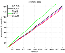
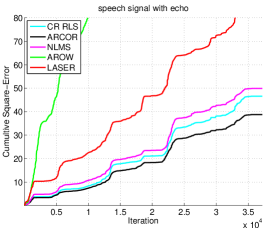
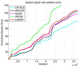
Figure 1: Cumulative squared loss for AROWR, ARCOR, LASER, NLMS and CR-RLS vs iteration. Left panel shows result for synthetic datasets with drift, and two right panels show results for a problem of acoustic echo cancelation on speech signal (best shown in color).

We evaluate our algorithms on three datasets, one synthetic and two real world. The synthetic dataset contains $2,000$ points in $\mathbb{R}^{20}$, where the first ten coordinates were grouped into five groups of size two. Each such pair was drawn from a $45^{\circ}$ rotated Gaussian distribution with standard deviations $10$ and $1$. The remaining $10$ coordinates were drawn from independent Gaussian distributions ${\mathcal{N}}\left({0,2}\right)$. The dataset was generated using a sequence of vectors ${\boldsymbol{u}}_{t}\in\mathbb{R}^{20}$ for which the only non-zero coordinates are the first two, where their values are the coordinates of a unit vector that is rotating with a constant rate. Specifically, we have $\|{\boldsymbol{u}}_{t}\|=1$ and the instantaneous drift $\|{\boldsymbol{u}}_{t}-{\boldsymbol{u}}_{t-1}\|$ is constant.

The other two datasets are generated from echoed speech signal. The first speech echoed signal was generated using FIR filter with $k$ delays and varying attenuated amplitude. This effect imitates acoustic echo reflections from large, distant and dynamic obstacles. The difference equation $y(n)=x(n)+\sum_{D=1}^{k}{A(n)x(n-D)}+v(n)$ was used, where $D$ is a delay in samples, the coefficient $A(n)$ describes the changing attenuation related from object reflection and $v(n)\sim{\mathcal{N}}\left({0,10^{-3}}\right)$ is a white noise. The second speech echoed signal was generated using a flange IIR filter, where the delay is not constat, but changing with time. This effect imitates time stretching of audio signal caused by moving and changing objects in the room. The difference equation $y(n)=x(n)+Ay\left({n-D(n)}\right)+v(n)$ was used.

Five algorithms are evaluated: NLMS (normalized least mean square) ([3, 4]) which is a state-of-the-art first-order algorithm, AROWR (AROW for Regression) with no restarts nor projection, ARCOR, LASER and CR-RLS. For the synthetic datasets the algorithms’ parameters were tuned using a single random sequence. We repeat each experiment $100$ times reporting the mean cumulative square-loss. We note that AAR ([21, 36]) is a special case of LASER and RLS is a special case of CR-RLS, for a specific choice of their respective parameters. Additionally, the performance of AROWR, AAR and RLS is similar, and thus only the performance of AROWR is shown. For the speech signal the algorithms’ parameters were tuned on $10\%$ of the signal, then the best parameter choices for each algorithm were used to evaluate the performance on the remaining signal.

The results are summarized in Fig. 1. AROWR performs worst on all datasets as it converges very fast and thus not able to track the changes in the data. Focusing on the left panel, showing the results for the synthetic signal, we observe that ARCOR performs relatively bad as suggested by our analysis for constant, yet not too large, drift. Both CR-RLS and NLMS perform better, where CR-RLS is slightly better as it is a second order algorithm, and allows to converge faster between switches. On the other hand, NLMS is not converging and is able to adapt to the drift. Finally, LASER performs the best, as hinted by its analysis, for which the bound is lower where there is a constant drift.

Moving to the center panel, showing the results for first echoed speech signal with varying amplitude, we observe that LASER is the worst among all algorithms except AROWR. Indeed, it does preventing convergence by keeping the learning rates far from zero, yet it is a min-max algorithm designed for the worst-case, which is not the case for real-world speech data. However, speech data is highly regular and the instantaneous drift vary. NLMS performs better as it is not converging, yet both CR-RLS and ARCOR perform even better, as they both not-converging due to covariance resets on the one hand, and second order updates on the other hand. ARCOR outperforms CR-RLS as the former adapts the resets to actual data, and is not using pre-defined scheduling as the later.

Finally, the right panel summarizes the results for evaluations on the second echoed speech signal. Note that the amount of drift grows since the data is generated using flange filter. Both LASER and ARCOR are out-performed as both assume drift that is sublinear or at most linear, which is not the case. CR-RLS outperforms NLMS. The later is first order, so is able to adapt to changes, yet has slower converge rate. The former is able to cope with drift due to resets.

Interestingly, in all experiments, NLMS was not performing the best nor the worst. There is no clear winner among the three algorithms that are both second order, and designed to adapt to drifts. Intuitively, if the drift suits the assumptions of an algorithm, that algorithm would perform the best, and otherwise, its performance may even be worse than of NLMS.

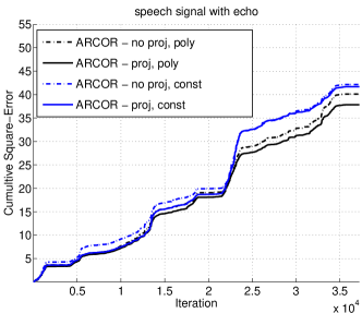
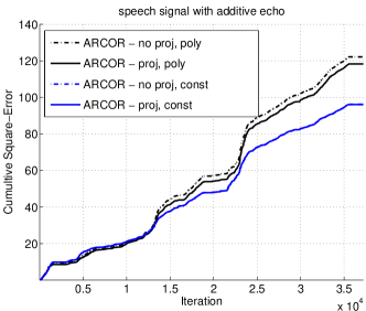
Figure 2: Cumulative squared loss of four variants of ARCOR vs iteration.

We have seen above that ARCOR performs a projection step, which partially was motivated from the analysis. We now evaluate its need and affect in practice on two speech problems. We test two modifications of ARCOR, resulting in four variants altogether. First, we replace the the polynomial thresholds scheme to the constant thresholds scheme, that is, all thresholds are equal. Second, we omit the projection step. The results are summarized in Fig. 2. The line corresponding to the original algorithm, is called “proj, poly” as it performs a projection step and uses polynomial schema for the lower-bound on eigenvalues. The version that omits projection and uses constant schema, called “no proj, const”, is most similar to CR-RLS. Both resets the covariance matrix, CR-RLS after fixed amount of iterations, while “ARCOR-no proj, const” when the eigenvalues meets a specified fixed lower bound. The difference between the two plots is the amount of drift used: the top panel shows results for sublinear drift, and the bottom panel shows results with increasing per-instance drift. The original version, as hinted by the analysis, is designed to work with sub-linear drift, and performs the best in this case. However, when this assumption over the amount of drift breaks, this version is not optimal anymore, and constat schema performs better, as it allows the algorithm to adapt to non-vanishing drift. Finally, in both datasets, the algorithm that perform best perform a projection step after each iteration. Providing some empirical evidence for its need.

VIII Summary and Conclusions

We proposed and analyzed two novel algorithms for non-stationary online regression designed and analyzed with the squared loss in the worst-case regret framework. The ARCOR algorithm was built on AROWR, that employs second order information, yet performs data-dependent covariance resets, which provides it the ability to track drifts. The LASER algorithm was built on the last-step minmax predictor with the proper modifications for non-stationary problems. Regret bounds shown and proven are optimized using knowledge on the amount of drift, and in general the two algorithms are not comparable.

Few open directions are possible. First, to extend these algorithms to other loss functions rather than the squared loss. Second, currently, direct implementation of both algorithms requires either matrix inversion or eigenvector decomposition. A possible direction is to design a more efficient version of these algorithms. Third, an interesting direction is to design algorithms that automatically detect the level of drift, or do not need this information before run-time.

-A Proof of Lemma 1

Proof:

We calculate

$$P_{t}\left({\boldsymbol{u}}_{t}\right)= \min_{{\boldsymbol{u}}_{1},\ldots,{\boldsymbol{u}}_{t-1}}\Bigg{(}b\left\|{\boldsymbol{u}}_{1}\right\|^{2}+c\sum_{s=1}^{t-1}\left\|{\boldsymbol{u}}_{s+1}-{\boldsymbol{u}}_{s}\right\|^{2}$$

$$+\sum_{s=1}^{t}\left(y_{s}-{{\boldsymbol{u}}}^{\top}_{s}{\boldsymbol{x}}_{s}\right)^{2}\Bigg{)}$$

$$= \min_{{\boldsymbol{u}}_{1},\ldots,{\boldsymbol{u}}_{t-1}}\Bigg{(}b\left\|{\boldsymbol{u}}_{1}\right\|^{2}+c\sum_{s=1}^{t-2}\left\|{\boldsymbol{u}}_{s+1}-{\boldsymbol{u}}_{s}\right\|^{2}$$

$$+\sum_{s=1}^{t-1}\left(y_{s}-{{\boldsymbol{u}}}^{\top}_{s}{\boldsymbol{x}}_{s}\right)^{2}+c\left\|{\boldsymbol{u}}_{t}-{\boldsymbol{u}}_{t-1}\right\|^{2}$$

$$+\left(y_{t}-{{\boldsymbol{u}}}^{\top}_{t}{\boldsymbol{x}}_{t}\right)^{2}\Bigg{)}$$

$$= \min_{{\boldsymbol{u}}_{t-1}}\min_{{\boldsymbol{u}}_{1},\ldots,{\boldsymbol{u}}_{t-2}}\Bigg{(}b\left\|{\boldsymbol{u}}_{1}\right\|^{2}+c\sum_{s=1}^{t-2}\left\|{\boldsymbol{u}}_{s+1}-{\boldsymbol{u}}_{s}\right\|^{2}$$

$$+\sum_{s=1}^{t-1}\left(y_{s}-{{\boldsymbol{u}}}^{\top}_{s}{\boldsymbol{x}}_{s}\right)^{2}+c\left\|{\boldsymbol{u}}_{t}-{\boldsymbol{u}}_{t-1}\right\|^{2}$$

$$+\left(y_{t}-{{\boldsymbol{u}}}^{\top}_{t}{\boldsymbol{x}}_{t}\right)^{2}\Bigg{)}$$

$$= \min_{{\boldsymbol{u}}_{t-1}}\Bigg{[}\min_{{\boldsymbol{u}}_{1},\ldots,{\boldsymbol{u}}_{t-2}}\bigg{(}b\left\|{\boldsymbol{u}}_{1}\right\|^{2}+c\sum_{s=1}^{t-2}\left\|{\boldsymbol{u}}_{s+1}-{\boldsymbol{u}}_{s}\right\|^{2}$$

$$+\sum_{s=1}^{t-1}\left(y_{s}-{{\boldsymbol{u}}}^{\top}_{s}{\boldsymbol{x}}_{s}\right)^{2}\bigg{)}$$

$$+c\left\|{\boldsymbol{u}}_{t}-{\boldsymbol{u}}_{t-1}\right\|^{2}+\left(y_{t}-{{\boldsymbol{u}}}^{\top}_{t}{\boldsymbol{x}}_{t}\right)^{2}\Bigg{]}$$

$$= \min_{{\boldsymbol{u}}_{t-1}}\Bigg{(}P_{t-1}\left({\boldsymbol{u}}_{t-1}\right)+c\left\|{\boldsymbol{u}}_{t}-{\boldsymbol{u}}_{t-1}\right\|^{2}$$

$$+\left(y_{t}-{{\boldsymbol{u}}}^{\top}_{t}{\boldsymbol{x}}_{t}\right)^{2}\Bigg{)}~{}.$$

∎

-B Proof of Lemma 2

Proof:

By definition,

$$P_{1}\left({\boldsymbol{u}}_{1}\right) =Q_{1}\left({\boldsymbol{u}}_{1}\right)=b\left\|{\boldsymbol{u}}_{1}\right\|^{2}+\left(y_{1}-{{\boldsymbol{u}}}^{\top}_{1}{\boldsymbol{x}}_{1}\right)^{2}$$

$$={{\boldsymbol{u}}}^{\top}_{1}\left(bI+{\boldsymbol{x}}_{1}{{\boldsymbol{x}}}^{\top}_{1}\right){\boldsymbol{u}}_{1}-2y_{1}{{\boldsymbol{u}}}^{\top}_{1}{\boldsymbol{x}}_{1}+y_{1}^{2}~{},$$

and indeed $D_{1}=bI+{\boldsymbol{x}}_{1}{{\boldsymbol{x}}}^{\top}_{1}$, ${\boldsymbol{e}}_{1}=y_{1}{\boldsymbol{x}}_{1}$, and $f_{1}=y_{1}^{2}$.

We proceed by induction, assume that, $P_{t-1}\left({\boldsymbol{u}}_{t-1}\right)={{\boldsymbol{u}}}^{\top}_{t-1}D_{t-1}{\boldsymbol{u}}_{t-1}-2{{\boldsymbol{u}}}^{\top}_{t-1}{\boldsymbol{e}}_{t-1}+f_{t-1}$.

Applying Lemma 1 we get,

$$P_{t}\left({\boldsymbol{u}}_{t}\right) =\min_{{\boldsymbol{u}}_{t-1}}\Bigg{(}{{\boldsymbol{u}}}^{\top}_{t-1}D_{t-1}{\boldsymbol{u}}_{t-1}-2{{\boldsymbol{u}}}^{\top}_{t-1}{\boldsymbol{e}}_{t-1}+f_{t-1}$$

$$\quad+c\left\|{\boldsymbol{u}}_{t}-{\boldsymbol{u}}_{t-1}\right\|^{2}+\left(y_{t}-{{\boldsymbol{u}}}^{\top}_{t}{\boldsymbol{x}}_{t}\right)^{2}\Bigg{)}$$

$$=\min_{{\boldsymbol{u}}_{t-1}}\Bigg{(}{{\boldsymbol{u}}}^{\top}_{t-1}\left(cI+D_{t-1}\right){\boldsymbol{u}}_{t-1}-2{{\boldsymbol{u}}}^{\top}_{t-1}\left(c{\boldsymbol{u}}_{t}+{\boldsymbol{e}}_{t-1}\right)$$

$$\quad+f_{t-1}+c\left\|{\boldsymbol{u}}_{t}\right\|^{2}+\left(y_{t}-{{\boldsymbol{u}}}^{\top}_{t}{\boldsymbol{x}}_{t}\right)^{2}\Bigg{)}$$

$$=-\left(c{\boldsymbol{u}}_{t}+{\boldsymbol{e}}_{t-1}\right)^{\top}\left(cI+D_{t-1}\right)^{-1}\left(c{\boldsymbol{u}}_{t}+{\boldsymbol{e}}_{t-1}\right)+f_{t-1}$$

$$\quad+c\left\|{\boldsymbol{u}}_{t}\right\|^{2}+\left(y_{t}-{{\boldsymbol{u}}}^{\top}_{t}{\boldsymbol{x}}_{t}\right)^{2}$$

$$={{\boldsymbol{u}}}^{\top}_{t}\left(cI+{\boldsymbol{x}}_{t}{{\boldsymbol{x}}}^{\top}_{t}-c^{2}\left(cI+D_{t-1}\right)^{-1}\right){\boldsymbol{u}}_{t}$$

$$\quad-2{{\boldsymbol{u}}}^{\top}_{t}\left[c\left(cI+D_{t-1}\right)^{-1}{\boldsymbol{e}}_{t-1}+y_{t}{\boldsymbol{x}}_{t}\right]$$

$$\quad-{\boldsymbol{e}}^{\top}_{t-1}\left(cI+D_{t-1}\right)^{-1}{\boldsymbol{e}}_{t-1}+f_{t-1}+y_{t}^{2}~{}.$$

Using the Woodbury identity we continue to develop the last equation,

$$={{\boldsymbol{u}}}^{\top}_{t}\left(cI+{\boldsymbol{x}}_{t}{{\boldsymbol{x}}}^{\top}_{t}-c^{2}\left[c^{-1}I-c^{-2}\left(D_{t-1}^{-1}+c^{-1}I\right)^{-1}\right]\right){\boldsymbol{u}}_{t}$$

$$\quad-2{{\boldsymbol{u}}}^{\top}_{t}\left[\left(I+c^{-1}D_{t-1}\right)^{-1}{\boldsymbol{e}}_{t-1}+y_{t}{\boldsymbol{x}}_{t}\right]$$

$$\quad-{\boldsymbol{e}}^{\top}_{t-1}\left(cI+D_{t-1}\right)^{-1}{\boldsymbol{e}}_{t-1}+f_{t-1}+y_{t}^{2}$$

$$={{\boldsymbol{u}}}^{\top}_{t}\left(\left(D_{t-1}^{-1}+c^{-1}I\right)^{-1}+{\boldsymbol{x}}_{t}{{\boldsymbol{x}}}^{\top}_{t}\right){\boldsymbol{u}}_{t}$$

$$\quad-2{{\boldsymbol{u}}}^{\top}_{t}\left[\left(I+c^{-1}D_{t-1}\right)^{-1}{\boldsymbol{e}}_{t-1}+y_{t}{\boldsymbol{x}}_{t}\right]$$

$$\quad-{\boldsymbol{e}}^{\top}_{t-1}\left(cI+D_{t-1}\right)^{-1}{\boldsymbol{e}}_{t-1}+f_{t-1}+y_{t}^{2}~{},$$

and indeed $D_{t}=\left(D_{t-1}^{-1}+c^{-1}I\right)^{-1}+{\boldsymbol{x}}_{t}{{\boldsymbol{x}}}^{\top}_{t}$, ${\boldsymbol{e}}_{t}=\left(I+c^{-1}D_{t-1}\right)^{-1}{\boldsymbol{e}}_{t-1}+y_{t}{\boldsymbol{x}}_{t}$ and, $f_{t}=f_{t-1}-{\boldsymbol{e}}^{\top}_{t-1}\left(cI+D_{t-1}\right)^{-1}{\boldsymbol{e}}_{t-1}+y_{t}^{2}$, as desired. ∎

-C Proof of Theorem 3

We prove the theorem in four steps. First, we state the following technical lemma, for which we define the following notation,

$$d_{t}\left({{\boldsymbol{z}},{\boldsymbol{v}}}\right)=({\boldsymbol{z}}-{\boldsymbol{v}})^{\top}\Sigma_{t}^{-1}({\boldsymbol{z}}-{\boldsymbol{v}})~{},~{}$$

$$d_{\tilde{t}}\left({{\boldsymbol{z}},{\boldsymbol{v}}}\right)=({\boldsymbol{z}}-{\boldsymbol{v}})^{\top}\tilde{\Sigma}_{t}^{-1}({\boldsymbol{z}}-{\boldsymbol{v}})~{},~{}$$

$$\chi_{t}={\boldsymbol{x}}_{t}^{\top}\Sigma_{t-1}{\boldsymbol{x}}_{t}~{}.$$

Second, we define a telescopic sum and in Lemma 14 prove a lower bound for each element. Third, in Lemma 15 we upper bound one term of the telescopic sum, and finally, in the fourth step we combine all these parts to conclude the proof. Let us start with the technical lemma.

Lemma 13

Let ${\tilde{{\boldsymbol{w}}}_{t}}$ and $\tilde{\Sigma}_{t}$ be defined in (9) and (10), then,

$$d_{t-1}\left({{\boldsymbol{w}}_{t-1},{\boldsymbol{u}}_{t-1}}\right)-d_{\tilde{t}}\left({\tilde{{\boldsymbol{w}}_{t}},{\boldsymbol{u}}_{t-1}}\right)=\frac{1}{r}\ell_{t}-\frac{1}{r}g_{t}-\frac{\ell_{t}\chi_{t}}{r\left({r+\chi_{t}}\right)}~{}.$$

where $\ell_{t}=\left({y_{t}-{{\boldsymbol{w}}}^{\top}_{t-1}{\boldsymbol{x}}_{t}}\right)^{2}$ and $g_{t}=\left({y_{t}-{{\boldsymbol{u}}}^{\top}_{t-1}{\boldsymbol{x}}_{t}}\right)^{2}$.

Proof:

We start by writing the distances explicitly

$$d_{t-1}\left({{\boldsymbol{w}}_{t-1},{\boldsymbol{u}}_{t-1}}\right)-d_{\tilde{t}}\left({\tilde{{\boldsymbol{w}}}_{t},{\boldsymbol{u}}_{t-1}}\right)$$

$$= -{\left({{\boldsymbol{u}}_{t-1}-\tilde{{\boldsymbol{w}}}_{t}}\right)}^{\top}\tilde{\Sigma}_{t}^{-1}\left({{\boldsymbol{u}}_{t-1}-\tilde{{\boldsymbol{w}}}_{t}}\right)$$

$$+{\left({{\boldsymbol{u}}_{t-1}-{\boldsymbol{w}}_{t-1}}\right)}^{\top}\Sigma_{t-1}^{-1}\left({{\boldsymbol{u}}_{t-1}-{\boldsymbol{w}}_{t-1}}\right)~{}.$$

Substituting ${\tilde{{\boldsymbol{w}}}_{t}}$ as appears in (10) the last equation becomes,

$$-{\left({{\boldsymbol{u}}_{t-1}-{\boldsymbol{w}}_{t-1}}\right)}^{\top}\tilde{\Sigma}_{t}^{-1}\left({{\boldsymbol{u}}_{t-1}-{\boldsymbol{w}}_{t-1}}\right)$$

$$+2({\boldsymbol{u}}_{t-1}-{\boldsymbol{w}}_{t-1})\tilde{\Sigma}_{t}^{-1}\Sigma_{t-1}{\boldsymbol{x}}_{t}\frac{(y_{t}-{{\boldsymbol{x}}}^{\top}_{t}{\boldsymbol{w}}_{t-1})}{r+{{\boldsymbol{x}}}^{\top}_{t}\Sigma_{t-1}{\boldsymbol{x}}_{t}}$$

$$-\left({\frac{(y_{t}-{{\boldsymbol{x}}}^{\top}_{t}{\boldsymbol{w}}_{t-1})}{r+{{\boldsymbol{x}}}^{\top}_{t}\Sigma_{t-1}{\boldsymbol{x}}_{t}}}\right)^{2}{{\boldsymbol{x}}}^{\top}_{t}\Sigma_{t-1}\tilde{\Sigma}_{t}^{-1}\Sigma_{t-1}{\boldsymbol{x}}_{t}$$

$$+{\left({{\boldsymbol{u}}_{t-1}-{\boldsymbol{w}}_{t-1}}\right)}^{\top}\Sigma_{t-1}^{-1}\left({{\boldsymbol{u}}_{t-1}-{\boldsymbol{w}}_{t-1}}\right)~{}.$$

Plugging $\tilde{\Sigma}_{t}$ as appears in (9) we get,

$$d_{t-1}\left({{\boldsymbol{w}}_{t-1},{\boldsymbol{u}}_{t-1}}\right)-d_{\tilde{t}}\left({\tilde{{\boldsymbol{w}}}_{t},{\boldsymbol{u}}_{t-1}}\right)$$

$$= -{\left({{\boldsymbol{u}}_{t-1}-{\boldsymbol{w}}_{t-1}}\right)}^{\top}\left({\Sigma_{t-1}^{-1}+\frac{1}{r}{\boldsymbol{x}}_{t}{{\boldsymbol{x}}}^{\top}_{t}}\right)\left({{\boldsymbol{u}}_{t-1}-{\boldsymbol{w}}_{t-1}}\right)$$

$$+2{({\boldsymbol{u}}_{t-1}\!-\!{\boldsymbol{w}}_{t-1})}^{\top}\!\!\left({\Sigma_{t-1}^{-1}\!+\!\frac{1}{r}{\boldsymbol{x}}_{t}{{\boldsymbol{x}}}^{\top}_{t}}\right)\Sigma_{t-1}\!{\boldsymbol{x}}_{t}\frac{(y_{t}\!-\!{{\boldsymbol{x}}}^{\top}_{t}{\boldsymbol{w}}_{t-1})}{r\!+\!{{\boldsymbol{x}}}^{\top}_{t}\Sigma_{t-1}{\boldsymbol{x}}_{t}}$$

$$-\frac{(y_{t}-{{\boldsymbol{x}}}^{\top}_{t}{\boldsymbol{w}}_{t-1})^{2}}{\left({r+{{\boldsymbol{x}}}^{\top}_{t}\Sigma_{t-1}{\boldsymbol{x}}_{t}}\right)^{2}}{{\boldsymbol{x}}}^{\top}_{t}\Sigma_{t-1}\left({\Sigma_{t-1}^{-1}+\frac{1}{r}{\boldsymbol{x}}_{t}{{\boldsymbol{x}}}^{\top}_{t}}\right)\Sigma_{t-1}{\boldsymbol{x}}_{t}$$

$$+{\left({{\boldsymbol{u}}_{t-1}-{\boldsymbol{w}}_{t-1}}\right)}^{\top}\Sigma_{t-1}^{-1}\left({{\boldsymbol{u}}_{t-1}-{\boldsymbol{w}}_{t-1}}\right)~{}.$$

Finally, we substitute $\ell_{t}=\left({y_{t}-{{\boldsymbol{x}}}^{\top}_{t}{\boldsymbol{w}}_{t-1}}\right)^{2}$ , $g_{t}=\left({y_{t}-{{\boldsymbol{x}}}^{\top}_{t}{\boldsymbol{u}}_{t-1}}\right)^{2}$ and, $\chi_{t}={{\boldsymbol{x}}}^{\top}_{t}\Sigma_{t-1}{\boldsymbol{x}}_{t}$. Rearranging the terms,

$$d_{t-1}\left({{\boldsymbol{w}}_{t-1},{\boldsymbol{u}}_{t-1}}\right)-d_{\tilde{t}}\left({\tilde{{\boldsymbol{w}}}_{t},{\boldsymbol{u}}_{t-1}}\right)$$

$$= -\frac{1}{r}\left({y_{t}-{{\boldsymbol{x}}}^{\top}_{t}{\boldsymbol{w}}_{t-1}-\left({y_{t}-{{\boldsymbol{x}}}^{\top}_{t}{\boldsymbol{u}}_{t-1}}\right)}\right)^{2}$$

$$-\frac{2\left({y_{t}\!-\!{{\boldsymbol{x}}}^{\top}_{t}{\boldsymbol{u}}_{t-1}\!-\!\left({y_{t}\!-\!{{\boldsymbol{x}}}^{\top}_{t}{\boldsymbol{w}}_{t-1}}\right)}\right)\left({y_{t}\!-\!{{\boldsymbol{x}}}^{\top}_{t}{\boldsymbol{w}}_{t-1}}\right)}{r+\chi_{t}}\!\left({1\!+\!\frac{\chi_{t}}{r}}\right)$$

$$-\frac{\ell_{t}\chi_{t}}{\left({r+\chi_{t}}\right)^{2}}\left({1+\frac{\chi_{t}}{r}}\right)$$

$$= -\frac{1}{r}\ell_{t}+2\left({y_{t}-{{\boldsymbol{x}}}^{\top}_{t}{\boldsymbol{w}}_{t-1}}\right)\left({y_{t}-{{\boldsymbol{x}}}^{\top}_{t}{\boldsymbol{u}}_{t-1}}\right)\frac{1}{r}-\frac{1}{r}g_{t}$$

$$+\frac{2\ell_{t}}{r+\chi_{t}}\left({1+\frac{\chi_{t}}{r}}\right)-\frac{\ell_{t}\chi_{t}}{r\left({r+\chi_{t}}\right)}$$

$$-2\frac{\left({y_{t}-{{\boldsymbol{x}}}^{\top}_{t}{\boldsymbol{w}}_{t-1}}\right)\left({y_{t}-{{\boldsymbol{x}}}^{\top}_{t}{\boldsymbol{u}}_{t-1}}\right)}{r+\chi_{t}}\left({1+\frac{\chi_{t}}{r}}\right)$$

$$= \frac{1}{r}\ell_{t}-\frac{1}{r}g_{t}-\frac{\ell_{t}\chi_{t}}{r\left({r+\chi_{t}}\right)}~{},$$

which completes the proof. ∎

We now define one element of the telescopic sum, and lower bound it,

Lemma 14

Denote by

$$\Delta_{t}=d_{t-1}\left({{\boldsymbol{w}}_{t-1},{\boldsymbol{u}}_{t-1}}\right)-d_{t}\left({{\boldsymbol{w}}_{t},{\boldsymbol{u}}_{t}}\right)$$

then

$$\Delta_{t} \geq\frac{1}{r}\left({\ell_{t}-g_{t}}\right)-\ell_{t}\frac{\chi_{t}}{r(r+\chi_{t})}$$

$$\quad+{{\boldsymbol{u}}}^{\top}_{t-1}\Sigma_{t-1}^{-1}{\boldsymbol{u}}_{t-1}-{{\boldsymbol{u}}}^{\top}_{t}\Sigma_{t}^{-1}{\boldsymbol{u}}_{t}-2R_{B}\Lambda_{i}^{-1}\|{\boldsymbol{u}}_{t-1}-{\boldsymbol{u}}_{t}\|$$

where $i-1$ is the number of restarts occurring before example $t$.

Proof:

We write $\Delta_{t}$ as a telescopic sum of four terms as follows,

$$\Delta_{t,1} =d_{t-1}\left({{\boldsymbol{w}}_{t-1},{\boldsymbol{u}}_{t-1}}\right)-d_{\tilde{t}}\left({\tilde{{\boldsymbol{w}}}_{t},{\boldsymbol{u}}_{t-1}}\right)$$

$$\Delta_{t,2} =d_{\tilde{t}}\left({\tilde{{\boldsymbol{w}}}_{t},{\boldsymbol{u}}_{t-1}}\right)-d_{t}\left({\tilde{{\boldsymbol{w}}}_{t},{\boldsymbol{u}}_{t-1}}\right)$$

$$\Delta_{t,3} =d_{t}\left({\tilde{{\boldsymbol{w}}}_{t},{\boldsymbol{u}}_{t-1}}\right)-d_{t}\left({{\boldsymbol{w}}_{t},{\boldsymbol{u}}_{t-1}}\right)$$

$$\Delta_{t,4} =d_{t}\left({{\boldsymbol{w}}_{t},{\boldsymbol{u}}_{t-1}}\right)-d_{t}\left({{\boldsymbol{w}}_{t},{\boldsymbol{u}}_{t}}\right)$$

We lower bound each of the four terms. Since the value of $\Delta_{t,1}$ was computed in Lemma 13, we start with the second term. If no reset occurs then $\Sigma_{t}=\tilde{\Sigma}_{t}$ and $\Delta_{t,2}=0$. Otherwise, we use the facts that $0\preceq\tilde{\Sigma_{t}}\preceq I$ and $\Sigma_{t}=I$, and get,

$$\Delta_{t,2} ={\left({\tilde{{\boldsymbol{w}}}_{t}-{\boldsymbol{u}}_{t-1}}\right)}^{\top}\tilde{\Sigma}_{t}^{-1}\left({\tilde{{\boldsymbol{w}}}_{t}-{\boldsymbol{u}}_{t-1}}\right)$$

$$\quad-{\left({\tilde{{\boldsymbol{w}}}_{t}-{\boldsymbol{u}}_{t-1}}\right)}^{\top}\Sigma_{t}^{-1}\left({\tilde{{\boldsymbol{w}}}_{t}-{\boldsymbol{u}}_{t-1}}\right)$$

$$\geq{\rm Tr}\left({{\left({\tilde{{\boldsymbol{w}}}_{t}-{\boldsymbol{u}}_{t-1}}\right){\left({\tilde{{\boldsymbol{w}}}_{t}-{\boldsymbol{u}}_{t-1}}\right)}^{\top}\left({I-I}\right)}}\right)=0~{}.$$

To summarize, $\Delta_{t,2}\geq 0$. We can lower bound $\Delta_{t,3}\geq 0$ by using the fact that ${\boldsymbol{w}}_{t}$ is a projection of $\tilde{{\boldsymbol{w}}}_{t}$ onto a closed set (a ball of radius $R_{B}$ around the origin), which by our assumption contains ${\boldsymbol{u}}_{t}$. Employing Corollary 3 of Herbster and Warmuth [23] we get, $d_{t}\left({\tilde{{\boldsymbol{w}}}_{t},{\boldsymbol{u}}_{t-1}}\right)\geq d_{t}\left({{\boldsymbol{w}}_{t},{\boldsymbol{u}}_{t-1}}\right)$ and thus $\Delta_{t,3}\geq 0$.

Finally, we lower bound for the fourth term $\Delta_{t,4}$,

$$\Delta_{t,4} ={\left({{\boldsymbol{w}}_{t}-{\boldsymbol{u}}_{t-1}}\right)}^{\top}\Sigma_{t}^{-1}\left({{\boldsymbol{w}}_{t}-{\boldsymbol{u}}_{t-1}}\right)$$

$$\quad-{\left({{\boldsymbol{w}}_{t}-{\boldsymbol{u}}_{t}}\right)}^{\top}\Sigma_{t}^{-1}\left({{\boldsymbol{w}}_{t}-{\boldsymbol{u}}_{t}}\right)$$ (34)

$$={{\boldsymbol{u}}}^{\top}_{t-1}\Sigma_{t}^{-1}{\boldsymbol{u}}_{t-1}-{{\boldsymbol{u}}}^{\top}_{t}\Sigma_{t}^{-1}{\boldsymbol{u}}_{t}-2{{\boldsymbol{w}}}^{\top}_{t}\Sigma_{t}^{-1}\left({{\boldsymbol{u}}_{t-1}-{\boldsymbol{u}}_{t}}\right)$$

We use Hölder inequality and then Cauchy-Schwartz inequality to get the following lower bound,

$$-2{{\boldsymbol{w}}}^{\top}_{t}\Sigma_{t}^{-1}\left({{\boldsymbol{u}}_{t-1}-{\boldsymbol{u}}_{t}}\right)=-2{\rm Tr}\left({\Sigma_{t}^{-1}\left({{\boldsymbol{u}}_{t-1}-{\boldsymbol{u}}_{t}}\right){{\boldsymbol{w}}}^{\top}_{t}}\right)$$

$$~{}~{}~{}~{}~{}~{}~{}\geq-2\lambda_{max}\left({\Sigma_{t}^{-1}}\right){{\boldsymbol{w}}}^{\top}_{t}\left({{\boldsymbol{u}}_{t-1}-{\boldsymbol{u}}_{t}}\right)$$

$$~{}~{}~{}~{}~{}~{}~{}\geq-2\lambda_{max}\left({\Sigma_{t}^{-1}}\right)\|{\boldsymbol{w}}_{t}\|\|{{\boldsymbol{u}}_{t-1}-{\boldsymbol{u}}_{t}}\|~{}.$$

Using the facts that $\|{\boldsymbol{w}}_{t}\|\leq R_{B}$ and that $\lambda_{max}\left({\Sigma_{t}^{-1}}\right)=1/\lambda_{min}\left({\Sigma_{t}}\right)\leq\Lambda_{i}^{-1}$, where $i$ is the current segment index, we get,

$$-2{{\boldsymbol{w}}}^{\top}_{t}\Sigma_{t}^{-1}\left({{\boldsymbol{u}}_{t-1}-{\boldsymbol{u}}_{t}}\right) \geq-2\Lambda_{i}^{-1}R_{B}\|{{\boldsymbol{u}}_{t-1}-{\boldsymbol{u}}_{t}}\|~{}.$$ (35)

Substituting (35) in (34) and using $\Sigma_{t}\preceq\Sigma_{t-1}$ a lower bound is obtained,

$$\Delta_{t,4}\geq ~{}{{\boldsymbol{u}}}^{\top}_{t-1}\Sigma_{t}^{-1}{\boldsymbol{u}}_{t-1}-{{\boldsymbol{u}}}^{\top}_{t}\Sigma_{t}^{-1}{\boldsymbol{u}}_{t}-2R_{B}\Lambda_{i}^{-1}\|{\boldsymbol{u}}_{t-1}-{\boldsymbol{u}}_{t}\|$$

$$\geq ~{}{{\boldsymbol{u}}}^{\top}_{t-1}\Sigma_{t-1}^{-1}{\boldsymbol{u}}_{t-1}-{{\boldsymbol{u}}}^{\top}_{t}\Sigma_{t}^{-1}{\boldsymbol{u}}_{t}$$

$$-2R_{B}\Lambda_{i}^{-1}\|{\boldsymbol{u}}_{t-1}-{\boldsymbol{u}}_{t}\|~{}.$$ (36)

Combining (36) with Lemma 13 concludes the proof. ∎

Next we state an upper bound that will appear in one of the summands of the telescopic sum,

Lemma 15

During the runtime of the ARCOR algorithm we have,

$$\sum_{t=t_{i}}^{t_{i}+T_{i}}\!\frac{\chi_{t}}{(\chi_{t}+r)}\!\leq\!\log{\left({\det{\left({\Sigma_{t_{i+1}-1}^{-1}}\right)}}\right)}\!=\!\log{\left({\det{\left({\left({\Sigma^{i}}\right)^{-1}}\right)}}\right)}~{}.$$

We remind the reader that $t_{i}$ is the first example index after the $i$th restart, and $T_{i}$ is the number of examples observed before the next restart. We also remind the reader the notation $\Sigma^{i}=\Sigma_{t_{i+1}-1}$ is the covariance matrix just before the next restart.

The proof of the lemma is similar to the proof of Lemma 4 by Crammer et. al. [12] and thus omitted. We now put all the pieces together and prove Theorem 3.

Proof:

We bound the sum $\sum_{t}\Delta_{t}$ from above and below, and start with an upper bound using the property of telescopic sum,

$$\sum_{t}\Delta_{t} =\sum_{t}\left({d_{t-1}\left({{\boldsymbol{w}}_{t-1},{\boldsymbol{u}}_{t-1}}\right)-d_{t}\left({{\boldsymbol{w}}_{t},{\boldsymbol{u}}_{t}}\right)}\right)$$

$$=d_{0}\left({{\boldsymbol{w}}_{0},{\boldsymbol{u}}_{0}}\right)-d_{T}\left({{\boldsymbol{w}}_{T},{\boldsymbol{u}}_{T}}\right)\leq{d_{0}\left({{\boldsymbol{w}}_{0},{\boldsymbol{u}}_{0}}\right)}~{}.$$ (37)

We compute a lower bound by applying Lemma 14,

$$\sum_{t}\Delta_{t}\geq\sum_{t}\Bigg{(}\frac{1}{r}\left({\ell_{t}-g_{t}}\right)-\ell_{t}\frac{\chi_{t}}{r(r+\chi_{t})}$$

$$\quad+{{\boldsymbol{u}}}^{\top}_{t-1}\Sigma_{t-1}^{-1}{\boldsymbol{u}}_{t-1}-{{\boldsymbol{u}}}^{\top}_{t}\Sigma_{t}^{-1}{\boldsymbol{u}}_{t}-2R_{B}\Lambda_{i(t)}^{-1}\|{\boldsymbol{u}}_{t-1}-{\boldsymbol{u}}_{t}\|\Bigg{)}~{},$$

where ${i(t)}$ is the number of restarts occurred before observing the $t$th example. Continuing to develop the last equation we obtain,

$$\sum_{t}\Delta_{t}\geq \frac{1}{r}\sum_{t}\ell_{t}-\frac{1}{r}\sum_{t}g_{t}-\sum_{t}\ell_{t}\frac{\chi_{t}}{r(r+\chi_{t})}$$

$$+\sum_{t}\Bigg{(}{{\boldsymbol{u}}}^{\top}_{t-1}\Sigma_{t-1}^{-1}{\boldsymbol{u}}_{t-1}-{{\boldsymbol{u}}}^{\top}_{t}\Sigma_{t}^{-1}{\boldsymbol{u}}_{t}\Bigg{)}$$

$$-\sum_{t}2R_{B}\Lambda_{i(t)}^{-1}\|{\boldsymbol{u}}_{t-1}-{\boldsymbol{u}}_{t}\|$$

$$= \frac{1}{r}\sum_{t}\ell_{t}-\frac{1}{r}\sum_{t}g_{t}-\sum_{t}\ell_{t}\frac{\chi_{t}}{r(r+\chi_{t})}$$

$$+{{\boldsymbol{u}}}^{\top}_{0}\Sigma_{0}^{-1}{\boldsymbol{u}}_{0}-{{\boldsymbol{u}}}^{\top}_{T}\Sigma_{T}^{-1}{\boldsymbol{u}}_{T}$$

$$-2R_{B}\sum_{t}\Lambda_{i(t)}^{-1}\|{\boldsymbol{u}}_{t-1}-{\boldsymbol{u}}_{t}\|~{}.$$ (38)

Combining (37) with (38) and using ${d_{0}\left({{\boldsymbol{w}}_{0},{\boldsymbol{u}}_{0}}\right)}={{\boldsymbol{u}}}^{\top}_{0}\Sigma_{0}^{-1}{\boldsymbol{u}}_{0}$ (as ${\boldsymbol{w}}_{0}={\boldsymbol{0}}$),

$$\frac{1}{r}\sum_{t}\ell_{t}-\frac{1}{r}\sum_{t}g_{t}-\sum_{t}\ell_{t}\frac{\chi_{t}}{r(r+\chi_{t})}-{{\boldsymbol{u}}}^{\top}_{T}\Sigma_{T}^{-1}{\boldsymbol{u}}_{T}$$

$$\quad-2R_{B}\sum_{t}\Lambda_{i(t)}^{-1}\|{\boldsymbol{u}}_{t-1}-{\boldsymbol{u}}_{t}\|\leq 0~{}.$$

Rearranging the terms of the last inequality,

$$\sum_{t} \ell_{t}\leq\sum_{t}g_{t}+\sum_{t}\ell_{t}\frac{\chi_{t}}{r+\chi_{t}}+r{{\boldsymbol{u}}}^{\top}_{T}\Sigma_{T}^{-1}{\boldsymbol{u}}_{T}$$

$$+2R_{B}r\sum_{t}\frac{1}{\Lambda_{i(t)}}\|{\boldsymbol{u}}_{t-1}-{\boldsymbol{u}}_{t}\|~{}.$$

Since $\|{\boldsymbol{w}}_{t}\|\leq R_{B}$ and we assume that $\|{\boldsymbol{x}}_{t}\|=1$ and $\sup_{t}|y_{t}|=Y$, we get that $\sup_{t}\ell_{t}\leq 2(R_{B}^{2}+Y^{2})$. Substituting the last inequality in Lemma 15, we bound the second term in the right-hand-side,

$$\sum_{t}\ell_{t}\frac{\chi_{t}}{r+\chi_{t}} =\sum_{i}^{n}\sum_{t=t_{i}}^{t_{i}+T_{i}}\ell_{t}\frac{\chi_{t}}{r+\chi_{t}}$$

$$\leq\sum_{i}^{n}\left({\sup_{t}\ell_{t}}\right)\log\det\left({\left({\Sigma^{i}}\right)^{-1}}\right)$$

$$\leq 2\left({R_{B}^{2}+Y^{2}}\right)\sum_{i}^{n}\log\det\left({\left({\Sigma^{i}}\right)^{-1}}\right)~{}.$$

which completes the proof. ∎

-D Proof of Lemma 7

Proof:

We first use the Woodbury equation to get the following two identities

$$D_{t}^{-1}=\left[\left(D_{t-1}^{-1}+c^{-1}I\right)^{-1}+{\boldsymbol{x}}_{t}{{\boldsymbol{x}}}^{\top}_{t}\right]^{-1}$$

$$\quad=D_{t-1}^{-1}+c^{-1}I-\frac{\left(D_{t-1}^{-1}+c^{-1}I\right){\boldsymbol{x}}_{t}{{\boldsymbol{x}}}^{\top}_{t}\left(D_{t-1}^{-1}+c^{-1}I\right)}{1+{{\boldsymbol{x}}}^{\top}_{t}\left(D_{t-1}^{-1}+c^{-1}I\right){\boldsymbol{x}}_{t}}$$

$$\left(I+c^{-1}D_{t-1}\right)^{-1}=I-c^{-1}\left(D_{t-1}^{-1}+c^{-1}I\right)^{-1}~{}.$$

Multiplying both identities with each other we get,

$$D_{t}^{-1}\left(I+c^{-1}D_{t-1}\right)^{-1}$$

$$=~{} \left[D_{t-1}^{-1}+c^{-1}I-\frac{\left(D_{t-1}^{-1}+c^{-1}I\right){\boldsymbol{x}}_{t}{{\boldsymbol{x}}}^{\top}_{t}\left(D_{t-1}^{-1}+c^{-1}I\right)}{1+{{\boldsymbol{x}}}^{\top}_{t}\left(D_{t-1}^{-1}+c^{-1}I\right){\boldsymbol{x}}_{t}}\right]$$

$$\left[I-c^{-1}\left(D_{t-1}^{-1}+c^{-1}I\right)^{-1}\right]=$$

$$=~{} D_{t-1}^{-1}-\frac{\left(D_{t-1}^{-1}+c^{-1}I\right){\boldsymbol{x}}_{t}{{\boldsymbol{x}}}^{\top}_{t}D_{t-1}^{-1}}{1+{{\boldsymbol{x}}}^{\top}_{t}\left(D_{t-1}^{-1}+c^{-1}I\right){\boldsymbol{x}}_{t}}~{},$$ (39)

and, similarly, we multiply the identities in the other order and get,

$$\left(I+c^{-1}D_{t-1}\right)^{-1}D_{t}^{-1}=$$

$$=~{} \left[I-c^{-1}\left(D_{t-1}^{-1}+c^{-1}I\right)^{-1}\right]\left[D_{t-1}^{-1}+c^{-1}I\vphantom{\frac{\left(D_{t-1}^{-1}+c^{-1}I\right){\boldsymbol{x}}_{t}{{\boldsymbol{x}}}^{\top}_{t}\left(D_{t-1}^{-1}+c^{-1}I\right)}{1+{{\boldsymbol{x}}}^{\top}_{t}\left(D_{t-1}^{-1}+c^{-1}I\right){\boldsymbol{x}}_{t}}}\right.$$

$$\left.-\frac{\left(D_{t-1}^{-1}+c^{-1}I\right){\boldsymbol{x}}_{t}{{\boldsymbol{x}}}^{\top}_{t}\left(D_{t-1}^{-1}+c^{-1}I\right)}{1+{{\boldsymbol{x}}}^{\top}_{t}\left(D_{t-1}^{-1}+c^{-1}I\right){\boldsymbol{x}}_{t}}\right]$$

$$=~{} D_{t-1}^{-1}-\frac{D_{t-1}^{-1}{\boldsymbol{x}}_{t}{{\boldsymbol{x}}}^{\top}_{t}\left(D_{t-1}^{-1}+c^{-1}I\right)}{1+{{\boldsymbol{x}}}^{\top}_{t}\left(D_{t-1}^{-1}+c^{-1}I\right){\boldsymbol{x}}_{t}}~{},$$ (40)

Finally, from (39) we get,

$$\left(I+c^{-1}D_{t-1}\right)^{-1}D_{t}^{-1}{\boldsymbol{x}}_{t}{{\boldsymbol{x}}}^{\top}_{t}D_{t}^{-1}\left(I+c^{-1}D_{t-1}\right)^{-1}-D_{t-1}^{-1}$$

$$\quad+\left(I+c^{-1}D_{t-1}\right)^{-1}\left[D_{t}^{-1}\left(I+c^{-1}D_{t-1}\right)^{-1}+c^{-1}I\right]$$

$$=~{} \left(I+c^{-1}D_{t-1}\right)^{-1}D_{t}^{-1}{\boldsymbol{x}}_{t}{{\boldsymbol{x}}}^{\top}_{t}D_{t}^{-1}\left(I+c^{-1}D_{t-1}\right)^{-1}$$

$$\quad-D_{t-1}^{-1}+\Bigg{[}I-c^{-1}\left(D_{t-1}^{-1}+c^{-1}I\right)^{-1}\Bigg{]}\Bigg{[}D_{t-1}^{-1}+c^{-1}I\vphantom{\frac{\left(D_{t-1}^{-1}+c^{-1}I\right){\boldsymbol{x}}_{t}{{\boldsymbol{x}}}^{\top}_{t}\left(D_{t-1}^{-1}+c^{-1}I\right)}{1+{{\boldsymbol{x}}}^{\top}_{t}\left(D_{t-1}^{-1}+c^{-1}I\right){\boldsymbol{x}}_{t}}}$$

$$\quad-\frac{\left(D_{t-1}^{-1}+c^{-1}I\right){\boldsymbol{x}}_{t}{{\boldsymbol{x}}}^{\top}_{t}D_{t-1}^{-1}}{1+{{\boldsymbol{x}}}^{\top}_{t}\left(D_{t-1}^{-1}+c^{-1}I\right){\boldsymbol{x}}_{t}}\Bigg{]}~{}.$$

We further develop the last equality and use (39) and (40) in the second equality below,

$$=~{} \left(I\!+\!c^{-1}D_{t-1}\right)^{-1}\!D_{t}^{-1}{\boldsymbol{x}}_{t}{{\boldsymbol{x}}}^{\top}_{t}D_{t}^{-1}\left(I\!+\!c^{-1}D_{t-1}\right)^{-1}\!-\!D_{t-1}^{-1}$$

$$+D_{t-1}^{-1}-\frac{D_{t-1}^{-1}{\boldsymbol{x}}_{t}{{\boldsymbol{x}}}^{\top}_{t}D_{t-1}^{-1}}{1+{{\boldsymbol{x}}}^{\top}_{t}\left(D_{t-1}^{-1}+c^{-1}I\right){\boldsymbol{x}}_{t}}$$

$$=~{} \left[D_{t-1}^{-1}-\frac{D_{t-1}^{-1}{\boldsymbol{x}}_{t}{{\boldsymbol{x}}}^{\top}_{t}\left(D_{t-1}^{-1}+c^{-1}I\right)}{1+{{\boldsymbol{x}}}^{\top}_{t}\left(D_{t-1}^{-1}+c^{-1}I\right){\boldsymbol{x}}_{t}}\right]{\boldsymbol{x}}_{t}{{\boldsymbol{x}}}^{\top}_{t}$$

$$\Bigg{[}D_{t-1}^{-1}\vphantom{\frac{\left(D_{t-1}^{-1}+c^{-1}I\right){\boldsymbol{x}}_{t}{{\boldsymbol{x}}}^{\top}_{t}D_{t-1}^{-1}}{1+{{\boldsymbol{x}}}^{\top}_{t}\left(D_{t-1}^{-1}+c^{-1}I\right){\boldsymbol{x}}_{t}}}-\frac{\left(D_{t-1}^{-1}+c^{-1}I\right){\boldsymbol{x}}_{t}{{\boldsymbol{x}}}^{\top}_{t}D_{t-1}^{-1}}{1+{{\boldsymbol{x}}}^{\top}_{t}\left(D_{t-1}^{-1}+c^{-1}I\right){\boldsymbol{x}}_{t}}\Bigg{]}$$

$$-\frac{D_{t-1}^{-1}{\boldsymbol{x}}_{t}{{\boldsymbol{x}}}^{\top}_{t}D_{t-1}^{-1}}{1+{{\boldsymbol{x}}}^{\top}_{t}\left(D_{t-1}^{-1}+c^{-1}I\right){\boldsymbol{x}}_{t}}$$

$$=~{} -\frac{{{\boldsymbol{x}}}^{\top}_{t}\left(D_{t-1}^{-1}+c^{-1}I\right){\boldsymbol{x}}_{t}D_{t-1}^{-1}{\boldsymbol{x}}_{t}{{\boldsymbol{x}}}^{\top}_{t}D_{t-1}^{-1}}{\left(1+{{\boldsymbol{x}}}^{\top}_{t}\left(D_{t-1}^{-1}+c^{-1}I\right){\boldsymbol{x}}_{t}\right)^{2}}~{}~{}\preceq~{}~{}0~{}.$$

∎

-E Derivations for Theorem 8

$$\left(y_{t}-\hat{y}_{t}\right)^{2}+\min_{{\boldsymbol{u}}_{1},\ldots,{\boldsymbol{u}}_{t-1}}Q_{t-1}\left({\boldsymbol{u}}_{1},\ldots,{\boldsymbol{u}}_{t-1}\right)$$

$$-\min_{{\boldsymbol{u}}_{1},\ldots,{\boldsymbol{u}}_{t}}Q_{t}\left({\boldsymbol{u}}_{1},\ldots,{\boldsymbol{u}}_{t}\right)$$

$$= \left(y_{t}-\hat{y}_{t}\right)^{2}-{\boldsymbol{e}}^{\top}_{t-1}D_{t-1}^{-1}{\boldsymbol{e}}_{t-1}+f_{t-1}+{\boldsymbol{e}}^{\top}_{t}D_{t}^{-1}{\boldsymbol{e}}_{t}-f_{t}$$

$$= \left(y_{t}-\hat{y}_{t}\right)^{2}-{\boldsymbol{e}}^{\top}_{t-1}D_{t-1}^{-1}{\boldsymbol{e}}_{t-1}$$

$$+\left(\left(I+c^{-1}D_{t-1}\right)^{-1}{\boldsymbol{e}}_{t-1}+y_{t}{\boldsymbol{x}}_{t}\right)^{\top}D_{t}^{-1}$$

$$~{}~{}~{}\left(\left(I+c^{-1}D_{t-1}\right)^{-1}\vphantom{\left(I+c^{-1}D_{t-1}\right)^{-1}}{\boldsymbol{e}}_{t-1}+y_{t}{\boldsymbol{x}}_{t}\right)$$

$$+{\boldsymbol{e}}^{\top}_{t-1}\left(cI+D_{t-1}\right)^{-1}{\boldsymbol{e}}_{t-1}-y_{t}^{2}~{},$$

where the last equality follows from (15) and (16). We proceed to develop the last equality,

$$= \left(y_{t}-\hat{y}_{t}\right)^{2}-{\boldsymbol{e}}^{\top}_{t-1}D_{t-1}^{-1}{\boldsymbol{e}}_{t-1}$$

$$+{\boldsymbol{e}}^{\top}_{t-1}\left(I+c^{-1}D_{t-1}\right)^{-1}D_{t}^{-1}\left(I+c^{-1}D_{t-1}\right)^{-1}{\boldsymbol{e}}_{t-1}$$

$$+2y_{t}{{\boldsymbol{x}}}^{\top}_{t}D_{t}^{-1}\left(I+c^{-1}D_{t-1}\right)^{-1}{\boldsymbol{e}}_{t-1}$$

$$+y_{t}^{2}{{\boldsymbol{x}}}^{\top}_{t}D_{t}^{-1}{\boldsymbol{x}}_{t}+{\boldsymbol{e}}^{\top}_{t-1}\left(cI+D_{t-1}\right)^{-1}{\boldsymbol{e}}_{t-1}-y_{t}^{2}$$

$$= \left(y_{t}-\hat{y}_{t}\right)^{2}+{\boldsymbol{e}}^{\top}_{t-1}\Bigg{(}-D_{t-1}^{-1}$$

$$+\left(I+c^{-1}D_{t-1}\right)^{-1}D_{t}^{-1}\Big{(}I+c^{-1}D_{t-1}\Big{)}^{-1}$$

$$+c^{-1}\left(I+c^{-1}D_{t-1}\right)^{-1}\Bigg{)}{\boldsymbol{e}}_{t-1}$$

$$+2y_{t}{{\boldsymbol{x}}}^{\top}_{t}D_{t}^{-1}\left(I\!+\!c^{-1}D_{t-1}\right)^{-1}{\boldsymbol{e}}_{t-1}\!+\!y_{t}^{2}{{\boldsymbol{x}}}^{\top}_{t}D_{t}^{-1}{\boldsymbol{x}}_{t}\!-\!y_{t}^{2}$$

$$= \left(y_{t}-\hat{y}_{t}\right)^{2}+{\boldsymbol{e}}^{\top}_{t-1}\Bigg{(}-D_{t-1}^{-1}+\Big{(}I\vphantom{\left[D_{t}^{-1}\left(I+c^{-1}D_{t-1}\right)^{-1}+c^{-1}I\right]}+c^{-1}D_{t-1}\Big{)}^{-1}$$

$$\left[D_{t}^{-1}\left(I+c^{-1}D_{t-1}\right)^{-1}+c^{-1}I\right]\Bigg{)}{\boldsymbol{e}}_{t-1}$$

$$+2y_{t}{{\boldsymbol{x}}}^{\top}_{t}D_{t}^{-1}\left(I\!+\!c^{-1}D_{t-1}\right)^{-1}{\boldsymbol{e}}_{t-1}\!+\!y_{t}^{2}{{\boldsymbol{x}}}^{\top}_{t}D_{t}^{-1}{\boldsymbol{x}}_{t}\!-\!y_{t}^{2}~{}.$$

-F Proof of Corollary 12

Proof:

Plugging Lemma 9 in Theorem 8 we have for all $({\boldsymbol{u}}_{1}\dots\boldsymbol{u}_{T})$,

$$L_{T}(\textrm{LASER})$$

$$\leq~{} b\left\|{\boldsymbol{u}}_{1}\right\|^{2}+cV^{(2)}+L_{T}(\{{\boldsymbol{u}}_{t}\})+Y^{2}\ln\left|\frac{1}{b}D_{T}\right|$$

$$+c^{-1}Y^{2}\sum_{t=1}^{T}{\rm Tr}\left({D_{t-1}}\right)$$

$$\leq~{} b\left\|{\boldsymbol{u}}_{1}\right\|^{2}+L_{T}(\{{\boldsymbol{u}}_{t}\})+Y^{2}\ln\left|\frac{1}{b}D_{T}\right|$$

$$+c^{-1}Y^{2}{\rm Tr}\left({D_{0}}\right)+cV^{(2)}$$

$$+c^{-1}Y^{2}Td\max\left\{{\!\!\frac{3X^{2}\!+\!\sqrt{X^{4}\!+\!4X^{2}c}}{2},b\!+\!X^{2}\!\!}\right\}~{},$$

where the last inequality follows from Lemma 11. The term $c^{-1}Y^{2}{\rm Tr}\left({D_{0}}\right)$ does not depend on $T$, because

$$c^{-1}Y^{2}{\rm Tr}\left({D_{0}}\right)=c^{-1}Y^{2}d\frac{bc}{c-b}=\frac{\varepsilon}{1-\varepsilon}Y^{2}d~{}.$$

To show (32), note that

$$V^{(2)}\leq T\frac{\sqrt{2}Y^{2}dX}{\mu^{3/2}}\Leftrightarrow\mu\leq\left({\frac{\sqrt{2}Y^{2}dXT}{V^{(2)}}}\right)^{2/3}=c~{}.$$

We thus have that the right term of (30) is upper bounded,

$$\max\left\{{\frac{3X^{2}+\sqrt{X^{4}+4X^{2}c}}{2},b+X^{2}}\right\}$$

$$\leq~{} \max\left\{{\frac{3X^{2}+\sqrt{8X^{2}c}}{2},b+X^{2}}\right\}$$

$$\leq~{} \max\left\{{\sqrt{8X^{2}c},b+X^{2}}\right\}\leq 2X\sqrt{2c}~{}.$$

Using this bound and plugging the value of $c$ from (31) we bound (30),

$$\left({\frac{\sqrt{2}TY^{2}dX}{V^{(2)}}}\right)^{2/3}V^{(2)}+Y^{2}Td2X\sqrt{2\left({\frac{\sqrt{2}TY^{2}dX}{V^{(2)}}}\right)^{-2/3}}$$

$$\quad=3\left({\sqrt{2}TY^{2}dX}\right)^{2/3}\left({V^{(2)}}\right)^{1/3}~{},$$

which concludes the proof. ∎

-G Details for the bound (33)

To show the bound (33), note that,

$$V^{(2)}\geq T\frac{Y^{2}dM}{\mu^{2}}\Leftrightarrow\mu\geq\sqrt{\frac{TY^{2}dM}{V^{(2)}}}=c~{}.$$

We thus have that the right term of (30) is upper bounded as follows,

$$\max\left\{{\frac{3X^{2}+\sqrt{X^{4}+4X^{2}c}}{2},b+X^{2}}\right\}$$

$$\leq~{} \max\left\{{3X^{2},\sqrt{X^{4}+4X^{2}c},b+X^{2}}\right\}$$

$$\leq~{} \max\left\{{3X^{2},\sqrt{2}X^{2},\sqrt{8X^{2}c},b+X^{2}}\right\}$$

$$=~{} \sqrt{8X^{2}}\max\left\{{\frac{3X^{2}}{\sqrt{8X^{2}}},\sqrt{c},\frac{b+X^{2}}{\sqrt{8X^{2}}}}\right\}$$

$$=~{} \sqrt{8X^{2}}\sqrt{\max\left\{{\frac{(3X^{2})^{2}}{{8X^{2}}},c,\frac{\left({b+X^{2}}\right)^{2}}{{8X^{2}}}}\right\}}$$

$$=~{} \sqrt{8X^{2}}\sqrt{\max\left\{{\mu,c}\right\}}\leq\sqrt{8X^{2}}\sqrt{\mu} =M~{}.$$

Using this bound and plugging $c=\sqrt{{Y^{2}dMT}/{V^{(2)}}}$ we bound (30), $\sqrt{\frac{Y^{2}dMT}{V^{(2)}}}V^{(2)}+\frac{1}{\sqrt{\frac{Y^{2}dMT}{V^{(2)}}}}TdY^{2}M=2\sqrt{Y^{2}dMTV^{(2)}}~{}.$

References

• [1] Peter Auer and Manfred K. Warmuth. Tracking the best disjunction. Electronic Colloquium on Computational Complexity (ECCC), 7(70), 2000.
• [2] K.S. Azoury and M.W. Warmuth. Relative loss bounds for on-line density estimation with the exponential family of distributions. Machine Learning, 43(3):211–246, 2001.
• [3] N. J. Bershad. Analysis of the normalized lms algorithm with gaussian inputs. IEEE Transactions on Acoustics, Speech, and Signal Processing, 34(4):793–806, 1986.
• [4] R. R. Bitmead and B. D. O. Anderson. Performance of adaptive estimation algorithms in dependent random environments. IEEE Transactions on Automatic Control, 25:788–794, 1980.
• [5] Steven Busuttil and Yuri Kalnishkan. Online regression competitive with changing predictors. In ALT, pages 181–195, 2007.
• [6] Giovanni Cavallanti, Nicolò Cesa-Bianchi, and Claudio Gentile. Tracking the best hyperplane with a simple budget perceptron. Machine Learning, 69(2-3):143–167, 2007.
• [7] Nicolo Ceas-Bianchi, Philip M. Long, and Manfred K. Warmuth. Worst case quadratic loss bounds for on-line prediction of linear functions by gradient descent. Technical Report IR-418, University of California, Santa Cruz, CA, USA, 1993.
• [8] Nicoló Cesa-Bianchi, Alex Conconi, and Claudio Gentile. A second-order perceptron algorithm. Siam Journal of Commutation, 34(3):640–668, 2005.
• [9] Nicolo Cesa-Bianchi and Gabor Lugosi. Prediction, Learning, and Games. Cambridge University Press, New York, NY, USA, 2006.
• [10] Min-Shin Chen and Jia-Yush Yen. Application of the least squares algorithm to the observer design for linear time-varying systems. Automatic Control, IEEE Transactions on, 44(9):1742 –1745, sep 1999.
• [11] K. Crammer, M. Dredze, and F. Pereira. Exact confidence-weighted learning. In NIPS 22, 2008.
• [12] K. Crammer, A. Kulesza, and M. Dredze. Adaptive regularization of weighted vectors. In Advances in Neural Information Processing Systems 23, 2009.
• [13] M. Dredze, K. Crammer, and F. Pereira. Confidence-weighted linear classification. In ICML, 2008.
• [14] John Duchi, Elad Hazan, and Yoram Singer. Adaptive subgradient methods for online learning and stochastic optimization. In COLT, pages 257–269, 2010.
• [15] A. Feuer and E. Weinstein. Convergence analysis of lms filters with uncorrelated gaussian data. IEEE Transactions on Acoustics, Speech, and Signal Processing, 33(1):222–230, 1985.
• [16] Jurgen Forster. On relative loss bounds in generalized linear regression. In Fundamentals of Computation Theory (FCT), 1999.
• [17] Dean P. Foster. Prediction in the worst case. The Annals of Statistics, 19(2):1084–1090, 1991.
• [18] Gene H. Golub and Charles F. Van Loan. Matrix computations (3rd ed.). Johns Hopkins University Press, Baltimore, MD, USA, 1996.
• [19] S.G. Goodhart, K.J. Burnham, and D.J.G. James”. Logical covariance matrix reset in self-tuning control. Mechatronics, 1(3):339 – 351, 1991.
• [20] G.C. Goodwin, E.K. Teoh, and H. Elliott. Deterministic convergence of a self-tuning regulator with covariance resetting. Control Theory and App., IEE Proc. D, 130(1):6 –8, 83.
• [21] Volodimir G.Vovk. Aggregating strategies. In Proceedings of the Third Annual Workshop on Computational Learning Theory, pages 371–383. Morgan Kaufmann, 1990.
• [22] Monson H. Hayes. 9.4: Recursive least squares. In Statistical Digital Signal Processing and Modeling, page 541, 1996.
• [23] Mark Herbster and Manfred K. Warmuth. Tracking the best linear predictor. Journal of Machine Learning Research, 1:281–309, 2001.
• [24] Rudolph Emil Kalman. A new approach to linear filtering and prediction problems. Transactions of the ASME–Journal of Basic Engineering, 82(Series D):35–45, 1960.
• [25] Jyrki Kivinen and Manfred K.Warmuth. Exponential gradient versus gradient descent for linear predictors. Information and Computation, 132:132–163, 1997.
• [26] Jyrki Kivinen, Alex J. Smola, and Robert C. Williamson. Online learning with kernels. In NIPS, pages 785–792, 2001.
• [27] Nick Littlestone and Manfred K. Warmuth. The weighted majority algorithm. Inf. Comput., 108(2):212–261, 1994.
• [28] H. Brendan McMahan and Matthew J. Streeter. Adaptive bound optimization for online convex optimization. In COLT, pages 244–256, 2010.
• [29] Edward Moroshko and Koby Crammer. Weighted last-step min-max algorithm with improved sub-logarithmic regret. In The 23nd International Conference on Algorithmic Learning Theory, ALT ’12, 2012.
• [30] Edward Moroshko and Koby Crammer. A last-step regression algorithm for non-stationary online learning. In AISTATS, 2013.
• [31] Mario E. Salgado, Graham C. Goodwin, and Richard H. Middleton. Modified least squares algorithm incorporating exponential resetting and forgetting. International Journal of Control, 47(2):477 –491, 1988.
• [32] Dan Simon. Optimal State Estimation: Kalman, H Infinity, and Nonlinear Approaches. Wiley-Interscience, 2006.
• [33] Hong-Seok Song, Kwanghee Nam, and P. Mutschler. Very fast phase angle estimation algorithm for a single-phase system having sudden phase angle jumps. In Industry Applications Conference. 37th IAS Annual Meeting, volume 2, pages 925 – 931, 2002.
• [34] Eiji Takimoto and Manfred K. Warmuth. The last-step minimax algorithm. In ALT, pages 279–290, 2000.
• [35] Nina Vaits and Koby Crammer. Re-adapting the regularization of weights for non-stationary regression. In The 22nd International Conference on Algorithmic Learning Theory, ALT ’11, 2011.
• [36] Volodya Vovk. Competitive on-line statistics. International Statistical Review, 69, 2001.
• [37] B. Widrow and Jr. M.E. Hoff. Adaptive switching circuits. 1960.