Quasi-likelihood for Spatial Point Processes

Abstract

Fitting regression models for intensity functions of spatial point processes is of great interest in ecological and epidemiological studies of association between spatially referenced events and geographical or environmental covariates. When Cox or cluster process models are used to accommodate clustering not accounted for by the available covariates, likelihood based inference becomes computationally cumbersome due to the complicated nature of the likelihood function and the associated score function. It is therefore of interest to consider alternative more easily computable estimating functions. We derive the optimal estimating function in a class of first-order estimating functions. The optimal estimating function depends on the solution of a certain Fredholm integral equation which in practice is solved numerically. The approximate solution is equivalent to a quasi-likelihood for binary spatial data and we therefore use the term quasi-likelihood for our optimal estimating function approach. We demonstrate in a simulation study and a data example that our quasi-likelihood method for spatial point processes is both statistically and computationally efficient.

1 INTRODUCTION

In many applications of spatial point processes it is of interest to fit a regression model for the intensity function. In case of a Poisson point process, maximum likelihood estimation of regression parameters is rather straightforward with a user-friendly implementation available in the R package spatstat. However, if Cox or cluster point process models are used to accommodate clustering not explained by a Poisson process, then maximum likelihood estimation is in general difficult from a computational point of view (see e.g. Møller and Waagepetersen, 2004). Alternatively, one may follow composite likelihood arguments (e.g. Møller and Waagepetersen, 2007) to obtain an estimating function that is equivalent to the score of the Poisson likelihood function. This provides a computationally tractable estimating function and theoretical properties of the resulting estimator are well understood, see e.g. Schoenberg (2005), Waagepetersen (2007) and Guan and Loh (2007).

A drawback of the Poisson score function approach is the loss of efficiency since possible dependence between points is ignored. In the context of intensity estimation, it appears that only Mrkvička and Molchanov (2005) and Guan and Shen (2010) have tried to incorporate second-order properties in the estimation so as to improve efficiency. Mrkvička and Molchanov (2005) show that their proposed estimator is optimal among a class of linear, unbiased intensity estimators, where the word ‘optimal’ refers to minimum variance. However, their approach is confined to a very restrictive type of intensity function known up to a one-dimensional scaling factor. In contrast, Guan and Shen (2010) propose a weighted estimating equation approach that is applicable to intensity functions in more general forms. A similar optimality result can on the other hand not be established for their approach.

In this paper we derive an optimal estimating function that not only takes into account possible spatial correlation but also is applicable for point processes with a general regression model for the intensity function. In the spirit of generalized linear models the intensity is given by a differentiable function of a linear predictor depending on spatial covariates. The optimal estimating function depends on the solution of a certain Fredholm integral equation and reduces to the likelihood score in case of a Poisson process. We show in Section 3.2 that the optimality result in Mrkvička and Molchanov (2005) is a special case of our more general result, and that the estimation method in Guan and Shen (2010) is only a crude approximation of our new approach. Apart from being computationally efficient, our estimating function only requires specification of the intensity function and the so-called pair correlation function, which is another advantage compared with maximum likelihood estimation.

For many types of correlated data other than spatial point patterns, estimating functions have been widely used for model fitting when maximum likelihood estimation is computationally challenging. Examples of such data include longitudinal data Liang and Zeger (1986), time series data Zeger (1988), clustered failure time data Gray (2003) and spatial binary or count data Gotway and Stroup (1997); Lin and Clayton (2005). For most of these methods, the inverse of a covariance matrix is used in their formulations as a way to account for the correlation in data, and optimality can be established when the so-called quasi-score estimating functions are used Heyde (1997). For point processes there is not a direct analogue of a spatial covariance matrix, but it turns out that a numerical implementation of our method is closely related to the quasi-likelihood for spatial data considered in Gotway and Stroup (1997) and Lin and Clayton (2005). Our work hence not only lays the theoretical foundation for optimal intensity estimation, but also fills in a critical gap between existing literature on spatial point processes and the well-established quasi-likelihood estimation method. We therefore adopt the term quasi-likelihood for our approach.

Following some background material on point processes and estimating functions, we derive our optimal estimating function and discuss the practical implementation of it based on a numerical solution of the Fredholm integral equation. Asymptotic properties of the resulting parameter estimator is then considered and the superior performance of the quasi-likelihood method compared with existing ones is demonstrated through a simulation study. We finally illustrate the practical use of the quasi-likelihood in a data example of three tropical tree species.

2 BACKGROUND

In this section we provide background on first- and second-order moments of spatial point processes, composite likelihood estimation and estimating functions. Throughout the presentation, we use ${\mathbb{E}}$, ${\mathbb{V}\mathrm{ar}}$ and ${\mathbb{C}\mathrm{ov}}$ to denote expectation, variance and covariance, respectively.

2.1 Intensity and Pair Correlation Function

Let $X$ be a point process on $\mathbb{R}^{2}$ and let $N(B)$ denote the number of points in $X\cap B$ for any bounded (Borel) set $B\subseteq\mathbb{R}^{2}$. We assume that $X$ has an intensity function $\lambda(\cdot)$ and a pair correlation function $g(\cdot,\cdot)$, whereby the first- and second-order moments of the counts $N(B)$ are given by

$${\mathbb{E}}N(B)=\int_{B}\lambda({\mathbf{u}})\mathrm{d}{\mathbf{u}}$$ (1)

and

$${\mathbb{C}\mathrm{ov}}[N(A),N(B)]=\int_{A\cap B}\lambda({\mathbf{u}})\mathrm{d}{\mathbf{u}}+\int_{A}\int_{B}\lambda({\mathbf{u}})\lambda({\mathbf{v}})[g({\mathbf{u}},{\mathbf{v}})-1]\mathrm{d}{\mathbf{u}}\mathrm{d}{\mathbf{v}}$$ (2)

for bounded sets $A,B\subseteq\mathbb{R}^{2}$ (Møller and Waagepetersen, 2004).

For convenience of exposition we assume that $g({\mathbf{u}},{\mathbf{v}})$ only depends on the difference ${\mathbf{u}}-{\mathbf{v}}$ since this is the common assumption in practice. In the following we thus let $g({\mathbf{r}})$ denote the pair correlation function for two points ${\mathbf{u}}$ and ${\mathbf{v}}$ with ${\mathbf{u}}-{\mathbf{v}}={\mathbf{r}}$. However, our proposed optimal estimating function is applicable also in the case of a non-translation invariant pair correlation function.

2.2 Composite Likelihood

Assume that the intensity function is given in terms of a parametric model $\lambda({\mathbf{u}})=\lambda({\mathbf{u}};{\boldsymbol{\beta}})$, where ${\boldsymbol{\beta}}=(\beta_{1},\ldots,\beta_{p})\in\mathbb{R}^{p}$ is a vector of regression parameters. Popular choices of the parametric model include linear and log linear models, $\lambda({\mathbf{u}};{\boldsymbol{\beta}})={\mathbf{z}}({\mathbf{u}}){\boldsymbol{\beta}}^{\mbox{\scriptsize\sf T}}$ and $\log\lambda({\mathbf{u}};{\boldsymbol{\beta}})={\mathbf{z}}({\mathbf{u}}){\boldsymbol{\beta}}^{\mbox{\scriptsize\sf T}}$, where ${\mathbf{z}}({\mathbf{u}})=(z_{1}({\mathbf{u}}),\ldots,z_{p}({\mathbf{u}}))$ is a covariate vector for each ${\mathbf{u}}\in\mathbb{R}^{2}$. A first-order log composite likelihood function Schoenberg (2005); Waagepetersen (2007) for estimation of ${\boldsymbol{\beta}}$ is given by

$$\sum_{{\mathbf{u}}\in X\cap W}\log\lambda({\mathbf{u}};{\boldsymbol{\beta}})-\int_{W}\lambda({\mathbf{u}};{\boldsymbol{\beta}})\mathrm{d}{\mathbf{u}},$$ (3)

where $W\subset\mathbb{R}^{2}$ is the observation window. This can be viewed as a limit of log composite likelihood functions for binary variables $Y_{i}=1[N(B_{i})>0]$, $i=1,\ldots,m$, where the cells $B_{i}$ form a disjoint partitioning of $W$ and $1[\cdot]$ is an indicator function (e.g. Møller and Waagepetersen, 2007). The limit is obtained when the number of cells tends to infinity and the areas of the cells tend to zero. In case of a Poisson process, the composite likelihood coincides with the likelihood function.

The composite likelihood is computationally simple and enjoys considerable popularity in particular in studies of tropical rain forest ecology where spatial point process models are fitted to huge spatial point pattern data sets of rain forest tree locations (see e.g. Shen et al., 2009; Lin et al., 2011). However, it is not statistically efficient for non-Poisson data since possible correlations between counts of points are ignored.

2.3 Primer on Estimating Functions

Referring to the previous Section 2.2, the composite likelihood estimator of ${\boldsymbol{\beta}}$ is obtained by maximizing the log composite likelihood (3). Assuming that $\lambda$ is differentiable with respect to ${\boldsymbol{\beta}}$ with gradient ${\boldsymbol{\lambda}}^{\prime}({\mathbf{u}};{\boldsymbol{\beta}})=\mathrm{d}\lambda({\mathbf{u}};{\boldsymbol{\beta}})/\mathrm{d}{\boldsymbol{\beta}}$, this is equivalent to solving the following equation:

$${\mathbf{e}}({\boldsymbol{\beta}})=\mathbf{0},$$ (4)

where

$${\mathbf{e}}({\boldsymbol{\beta}})=\sum_{{\mathbf{u}}\in X\cap W}\frac{{\boldsymbol{\lambda}}^{\prime}({\mathbf{u}};{\boldsymbol{\beta}})}{\lambda({\mathbf{u}};{\boldsymbol{\beta}})}-\int_{W}{\boldsymbol{\lambda}}^{\prime}({\mathbf{u}};{\boldsymbol{\beta}})\mathrm{d}{\mathbf{u}}$$ (5)

is the gradient of (3) with respect to ${\boldsymbol{\beta}}$. Equations in the form of (4) are typically referred to as estimating equations and functions like ${\mathbf{e}}({\boldsymbol{\beta}})$ are called estimating functions (Heyde, 1997). Note that many other statistical estimation procedures, such as maximum likelihood estimation, moment based estimation and minimum contrast estimation, can all be written in terms of estimating functions.

We defer rigorous asymptotic details to Section 5 and here just provide an informal overview of properties of an estimator $\hat{\boldsymbol{\beta}}$ based on an estimating function ${\mathbf{e}}({\boldsymbol{\beta}})$. By a first-order Taylor series expansion at $\hat{\boldsymbol{\beta}}$,

$${\mathbf{e}}({\boldsymbol{\beta}})\approx{\mathbf{e}}(\hat{\boldsymbol{\beta}})+[\hat{\boldsymbol{\beta}}-{\boldsymbol{\beta}}]{\mathbf{S}}=(\hat{\boldsymbol{\beta}}-{\boldsymbol{\beta}}){\mathbf{S}},$$

where ${\mathbf{S}}=-{\mathbb{E}}{\mathrm{d}{\mathbf{e}}({\boldsymbol{\beta}})}/{\mathrm{d}{\boldsymbol{\beta}}^{\mbox{\scriptsize\sf T}}}$ is the so-called sensitivity matrix (e.g. page 62 in Song, 2007) and the equality is due to ${\mathbf{e}}(\hat{\boldsymbol{\beta}})=\mathbf{0}$ as required by (4). It then follows immediately that $\hat{\boldsymbol{\beta}}\approx{\boldsymbol{\beta}}+{\mathbf{e}}({\boldsymbol{\beta}}){\mathbf{S}}^{-1}$. Thus, with ${\boldsymbol{\beta}}$ equal to the true parameter value, $\hat{\boldsymbol{\beta}}$ is approximately unbiased if ${\mathbb{E}}{\mathbf{e}}({\boldsymbol{\beta}})=0$, i.e. ${\mathbf{e}}({\boldsymbol{\beta}})$ is an unbiased estimating function. Moreover, ${\mathbb{V}\mathrm{ar}}\hat{\boldsymbol{\beta}}\approx{\mathbf{S}}^{-1}{\boldsymbol{\Sigma}}{\mathbf{S}}^{-1}$ where ${\boldsymbol{\Sigma}}={\mathbb{V}\mathrm{ar}}{\mathbf{e}}({\boldsymbol{\beta}})$ and ${\mathbf{S}}^{-1}{\boldsymbol{\Sigma}}{\mathbf{S}}^{-1}$ is the asymptotic covariance matrix when the size of the data set goes to infinity in a suitable manner (Section 5). The inverse of ${\mathbf{S}}^{-1}{\boldsymbol{\Sigma}}{\mathbf{S}}^{-1}$, i.e. ${\mathbf{S}}{\boldsymbol{\Sigma}}^{-1}{\mathbf{S}}$, is called the Godambe information (e.g. Definition 3.7 in Song, 2007).

Suppose that two competing estimating functions ${\mathbf{e}}_{1}({\boldsymbol{\beta}})$ and ${\mathbf{e}}_{2}({\boldsymbol{\beta}})$ with respective Godambe informations ${\mathbf{I}}_{1}$ and ${\mathbf{I}}_{2}$ are used to obtain the estimators $\hat{\boldsymbol{\beta}}_{1}$ and $\hat{\boldsymbol{\beta}}_{2}$. Then ${\mathbf{e}}_{1}({\boldsymbol{\beta}})$ is said to be superior to ${\mathbf{e}}_{2}({\boldsymbol{\beta}})$ if ${\mathbf{I}}_{1}-{\mathbf{I}}_{2}$ is positive definite, since this essentially means that $\hat{\boldsymbol{\beta}}_{1}$ has a smaller asymptotic variance than $\hat{\boldsymbol{\beta}}_{2}$. If ${\mathbf{I}}_{1}-{\mathbf{I}}_{2}$ is positive definite for all possible ${\mathbf{e}}_{2}({\boldsymbol{\beta}})$, then we say that ${\mathbf{e}}_{1}({\boldsymbol{\beta}})$ has the maximal Godambe information and is an optimal estimating function. The resulting estimator $\hat{\boldsymbol{\beta}}_{1}$ is then the asymptotically most efficient.

3 AN OPTIMAL FIRST-ORDER ESTIMATING EQUATION

The estimating function given in (5) can be rewritten as

$${\mathbf{e}}_{\mathbf{f}}({\boldsymbol{\beta}})=\sum_{{\mathbf{u}}\in X\cap W}{\mathbf{f}}({\mathbf{u}})-\int_{W}{\mathbf{f}}({\mathbf{u}})\lambda({\mathbf{u}};{\boldsymbol{\beta}})\mathrm{d}{\mathbf{u}},$$ (6)

where ${\mathbf{f}}({\mathbf{u}})={\boldsymbol{\lambda}}^{\prime}({\mathbf{u}};{\boldsymbol{\beta}})/\lambda({\mathbf{u}};{\boldsymbol{\beta}})$. In general, ${\mathbf{f}}({\mathbf{u}})$ can be any $1\times p$ real vector valued function, where $p$ is the dimension of ${\boldsymbol{\beta}}$. We call (6) a first-order estimating function. Our aim is to find a function ${\boldsymbol{\phi}}$ so that ${\mathbf{e}}_{{\boldsymbol{\phi}}}$ is optimal within the class of first-order estimating functions; in other words, the resulting estimator of ${\boldsymbol{\beta}}$ associated with ${\mathbf{e}}_{{\boldsymbol{\phi}}}$ is asymptotically most efficient.

Let ${\boldsymbol{\Sigma}}_{\mathbf{f}}={\mathbb{V}\mathrm{ar}}{\mathbf{e}}_{\mathbf{f}}({\boldsymbol{\beta}})$, ${\mathbf{J}}_{\mathbf{f}}=-\mathrm{d}{\mathbf{e}}_{\mathbf{f}}({\boldsymbol{\beta}})/\mathrm{d}{\boldsymbol{\beta}}^{\mbox{\scriptsize\sf T}}$ and ${\mathbf{S}}_{\mathbf{f}}={\mathbb{E}}{\mathbf{J}}_{\mathbf{f}}$. Note that ${\boldsymbol{\Sigma}}_{\mathbf{f}}$, ${\mathbf{J}}_{\mathbf{f}}$ and ${\mathbf{S}}_{\mathbf{f}}$ all depend on ${\boldsymbol{\beta}}$ but we suppress this dependence in this section for ease of presentation. Recalling the definition of optimality in Section 2.3, for ${\mathbf{e}}_{{\boldsymbol{\phi}}}$ to be optimal we must have that

$${\mathbf{S}}_{\boldsymbol{\phi}}{\boldsymbol{\Sigma}}_{\boldsymbol{\phi}}^{-1}{\mathbf{S}}_{\boldsymbol{\phi}}-{\mathbf{S}}_{\mathbf{f}}{\boldsymbol{\Sigma}}_{\mathbf{f}}^{-1}{\mathbf{S}}_{\mathbf{f}}$$ (7)

is non-negative definite for all ${\mathbf{f}}:W\to\mathbb{R}^{p}$. A sufficient condition for this is

$${\boldsymbol{\Sigma}}_{{\boldsymbol{\phi}}{\mathbf{f}}}={\mathbf{S}}_{\mathbf{f}}\$$ (8)

for all ${\mathbf{f}}$ where ${\boldsymbol{\Sigma}}_{{\mathbf{f}}{\boldsymbol{\phi}}}={\mathbb{C}\mathrm{ov}}[{\mathbf{e}}_{\mathbf{f}}({\boldsymbol{\beta}}),{\mathbf{e}}_{\boldsymbol{\phi}}({\boldsymbol{\beta}})]$. This type of condition is provided in Theorem 2.1 in Heyde (1997) for discrete or continuous vector-valued data. In Appendix A, we give a short self-contained proof of the sufficiency of (8) in our setting.

By the Campbell formulae (e.g. Møller and Waagepetersen, 2004, Chapter 4),

$${\boldsymbol{\Sigma}}_{{\boldsymbol{\phi}}{\mathbf{f}}} =\!\!\int_{W}\!\!\!{\mathbf{f}}^{\mbox{\scriptsize\sf T}}({\mathbf{u}}){\boldsymbol{\phi}}({\mathbf{u}})\lambda({\mathbf{u}};{\boldsymbol{\beta}})\mathrm{d}{\mathbf{u}}+\!\int_{W^{2}}\!\!\!\!\!{\mathbf{f}}^{\mbox{\scriptsize\sf T}}({\mathbf{u}}){\boldsymbol{\phi}}({\mathbf{v}})\lambda({\mathbf{u}};{\boldsymbol{\beta}})\lambda({\mathbf{v}};{\boldsymbol{\beta}})[g({\mathbf{u}}-{\mathbf{v}})-1]\mathrm{d}{\mathbf{u}}\mathrm{d}{\mathbf{v}},$$

$${\mathbf{S}}_{\mathbf{f}} =\int_{W}{\mathbf{f}}^{\mbox{\scriptsize\sf T}}({\mathbf{u}}){\boldsymbol{\lambda}}^{\prime}({\mathbf{u}};{\boldsymbol{\beta}})\mathrm{d}{\mathbf{u}}.$$

Hence, (8) is equivalent to

$$\int_{W}{\mathbf{f}}^{\mbox{\scriptsize\sf T}}({\mathbf{u}})\big{\{}{\boldsymbol{\lambda}}^{\prime}({\mathbf{u}};{\boldsymbol{\beta}})-{\boldsymbol{\phi}}({\mathbf{u}})\lambda({\mathbf{u}};{\boldsymbol{\beta}})-\lambda({\mathbf{u}};{\boldsymbol{\beta}})\int_{W}\phi({\mathbf{v}})\lambda({\mathbf{v}};{\boldsymbol{\beta}})[g({\mathbf{u}}-{\mathbf{v}})-1]\mathrm{d}{\mathbf{v}}\big{\}}\mathrm{d}{\mathbf{u}}={\bf 0}$$

for all ${\mathbf{f}}:W\to\mathbb{R}^{p}$, which is true if

$${\boldsymbol{\lambda}}^{\prime}({\mathbf{u}};{\boldsymbol{\beta}})-{\boldsymbol{\phi}}({\mathbf{u}})\lambda({\mathbf{u}};{\boldsymbol{\beta}})-\lambda({\mathbf{u}};{\boldsymbol{\beta}})\int_{W}\phi({\mathbf{v}})\lambda({\mathbf{v}};{\boldsymbol{\beta}})[g({\mathbf{u}}-{\mathbf{v}})-1]\mathrm{d}{\mathbf{v}}=0$$ (9)

for all ${\mathbf{u}}\in W$. Assuming $\lambda>0$, (9) implies that ${\boldsymbol{\phi}}$ is a solution to the Fredholm integral equation (e.g. Hackbusch, 1995, Chapter 3)

$${\boldsymbol{\phi}}=\frac{{\boldsymbol{\lambda}}^{\prime}}{\lambda}-{\mathbf{T}}{\boldsymbol{\phi}},$$ (10)

where ${\mathbf{T}}$ is the operator given by

$$({\mathbf{T}}{\mathbf{f}})({\mathbf{u}})=\int_{W}t({\mathbf{u}},{\mathbf{v}}){\mathbf{f}}({\mathbf{v}})\mathrm{d}{\mathbf{v}}\ \text{ with }\ t({\mathbf{u}},{\mathbf{v}})=\lambda({\mathbf{v}};{\boldsymbol{\beta}})[g({\mathbf{u}}-{\mathbf{v}})-1].$$ (11)

Assume that $g$ is continuous so that ${\mathbf{T}}$ is compact in the space of continuous functions on $W$ (Hackbusch, 1995, Theorem 3.2.5) and moreover that $-1$ is not an eigenvalue (we return to this condition in the next section). It then follows by Theorem 3.2.1 in Hackbusch (1995) that (10) has a unique solution

$${\boldsymbol{\phi}}=({\mathbf{I}}+{\mathbf{T}})^{-1}\frac{{\boldsymbol{\lambda}}^{\prime}}{\lambda},$$

where ${\mathbf{I}}$ is the identity operator (or, depending on context, the identity matrix) and $({\mathbf{I}}+{\mathbf{T}})^{-1}$ is the bounded linear inverse of ${\mathbf{I}}+{\mathbf{T}}$. We define

$${\mathbf{e}}({\boldsymbol{\beta}}) ={\mathbf{e}}_{\boldsymbol{\phi}}({\boldsymbol{\beta}})=\sum_{{\mathbf{u}}\in X\cap W}{\boldsymbol{\phi}}({\mathbf{u}})-\int_{W}{\boldsymbol{\phi}}({\mathbf{u}})\lambda({\mathbf{u}};{\boldsymbol{\beta}})\mathrm{d}{\mathbf{u}},$$ (12)

$${\boldsymbol{\Sigma}} ={\mathbb{V}\mathrm{ar}}{\mathbf{e}}({\boldsymbol{\beta}}),\,{\mathbf{J}}=-\mathrm{d}{\mathbf{e}}({\boldsymbol{\beta}})/\mathrm{d}{\boldsymbol{\beta}}^{\mbox{\scriptsize\sf T}},\,{\mathbf{S}}={\mathbb{E}}{\mathbf{J}}$$

where by the above derivations,

$${\mathbf{S}}={\boldsymbol{\Sigma}}=\int_{W}{\boldsymbol{\phi}}^{\mbox{\scriptsize\sf T}}({\mathbf{u}}){\boldsymbol{\lambda}}^{\prime}({\mathbf{u}};{\boldsymbol{\beta}})\mathrm{d}{\mathbf{u}}.$$ (13)

In the Poisson process case where $g(\cdot)=1$, (12) reduces to the Poisson likelihood score (5).

We develop a more explicit expression for ${\boldsymbol{\phi}}$ by using Neumann series expansion in Appendix B. The Neumann series expansion is also useful for checking the conditions for our asymptotic results; see Appendix C. However, it is not essential for our approach so we omit the detailed discussion here.

3.1 Condition for non-negative eigenvalues of ${\mathbf{T}}$

In general it is difficult to assess the eigenvalues of ${\mathbf{T}}$ given by (11). However, suppose that $g-1$ is non-negative definite so that ${\mathbf{T}}^{s}$ is a positive operator (i.e., $\int_{W}{\mathbf{f}}^{{\mbox{\scriptsize\sf T}}}({\mathbf{u}})({\mathbf{T}}^{s}{\mathbf{f}})({\mathbf{u}})\mathrm{d}{\mathbf{u}}\geq 0$) where ${\mathbf{T}}^{s}$ is given by the symmetric kernel

$$t^{s}({\mathbf{u}},{\mathbf{v}})=\lambda({\mathbf{u}};{\boldsymbol{\beta}})^{1/2}\lambda({\mathbf{v}};{\boldsymbol{\beta}})^{1/2}\big{[}g({\mathbf{u}}-{\mathbf{v}})-1\big{]}.$$

Then all eigenvalues of ${\mathbf{T}}^{s}$ are non-negative (Lax, 2002, Corollary 1, p. 320). In particular, $-1$ is not an eigenvalue. The same holds for ${\mathbf{T}}$ since it is easy to see that the eigenvalues of ${\mathbf{T}}$ coincide with those of ${\mathbf{T}}^{s}$.

The assumption of a non-negative definite $g(\cdot)-1$ is valid for the wide class of Cox point processes which in turn includes the class of Poisson cluster processes. For a Cox process driven by a random intensity function $\Lambda$, $g(u,v)=1+{\mathbb{C}\mathrm{ov}}[\Lambda({\mathbf{u}}),\Lambda({\mathbf{v}})]/[\lambda({\mathbf{u}})\lambda({\mathbf{v}})]$ so that $g(\cdot)-1$ is non-negative definite.

3.2 Relation to Existing Methods

Suppose we approximate the operator ${\mathbf{T}}$ by

$$({\mathbf{T}}{\mathbf{f}})({\mathbf{u}})=\int_{W}{\mathbf{f}}({\mathbf{v}})\lambda({\mathbf{v}};{\boldsymbol{\beta}})[g({\mathbf{u}}-{\mathbf{v}})-1)]\mathrm{d}{\mathbf{v}}\approx\lambda({\mathbf{u}};{\boldsymbol{\beta}}){\mathbf{f}}({\bf u})\int_{W}[g({\mathbf{u}}-{\mathbf{v}})-1]\mathrm{d}{\mathbf{v}}.$$ (14)

This is justified if ${\mathbf{f}}({\mathbf{v}})\lambda({\mathbf{v}};{\boldsymbol{\beta}})$ is close to ${\mathbf{f}}({\mathbf{u}})\lambda({\mathbf{u}};{\boldsymbol{\beta}})$ for the ${\mathbf{v}}$ where $g({\mathbf{u}}-{\mathbf{v}})-1$ differs substantially from zero. Then the Fredholm integral equation (10) can be approximated by

$${\boldsymbol{\phi}}=\frac{{\boldsymbol{\lambda}}^{\prime}}{\lambda}-\lambda A{\boldsymbol{\phi}},$$

where

$$A({\mathbf{u}})=\int_{W}\big{[}g({\mathbf{u}}-{\mathbf{v}})-1\big{]}\mathrm{d}{\mathbf{v}}.$$

We hence obtain an approximate solution ${\boldsymbol{\phi}}=w{\boldsymbol{\lambda}}^{\prime}/\lambda$ with $w({\mathbf{u}})=[1+\lambda({\mathbf{u}};{\boldsymbol{\beta}})A({\mathbf{u}})]^{-1}$. Using this approximation in (12) we obtain the estimating function

$$\sum_{{\mathbf{u}}\in X\cap W}w({\mathbf{u}})\frac{{\boldsymbol{\lambda}}^{\prime}({\mathbf{u}};{\boldsymbol{\beta}})}{\lambda({\mathbf{u}};{\boldsymbol{\beta}})}-\int_{W}w({\mathbf{u}}){\boldsymbol{\lambda}}^{\prime}({\mathbf{u}};{\boldsymbol{\beta}})\mathrm{d}{\mathbf{u}},$$

which is precisely the weighted Poisson score suggested in Guan and Shen (2010).

Mrkvička and Molchanov (2005) derived optimal intensity estimators in the situation of $\lambda({\mathbf{u}};\rho)=\rho\gamma({\mathbf{u}})$ for some known function $\gamma({\mathbf{u}})$ and unknown parameter $\rho>0$. Since $\rho$ is the only unknown parameter, a direct application of (10) yields

$$\rho{\boldsymbol{\phi}}({\mathbf{u}})+\rho^{2}\int_{W}{\boldsymbol{\phi}}({\mathbf{v}})\gamma({\mathbf{v}})\big{[}g({\mathbf{u}}-{\mathbf{v}})-1\big{]}\mathrm{d}{\mathbf{v}}=1,$$

which is essentially Corollary 3.1 of Mrkvička and Molchanov (2005). It is uncommon for an intensity function to be known up to a one-dimensional scaling factor. In contrast, our proposed modeling framework for the intensity function closely mimics that used in classical regression analysis and is more general. As a result, our method of derivation is completely different from that in Mrkvička and Molchanov (2005).

4 IMPLEMENTATION

In this section we discuss practical issues concerning the implementation of our proposed optimal estimating function. In particular we show in Section 4.2 that a particular numerical approximation of our optimal estimating function is equivalent to a quasi-likelihood for binary spatial data for which an iterative generalized least squares solution can be implemented. An R implementation will appear in future releases of spatstat.

4.1 Numerical Approximation

To estimate ${\boldsymbol{\phi}}$, consider the numerical approximation

$$({\mathbf{T}}{\boldsymbol{\phi}})({\mathbf{u}})=\int_{W}t({\mathbf{u}},{\mathbf{v}}){\boldsymbol{\phi}}({\mathbf{v}})\mathrm{d}{\mathbf{v}}\approx\sum_{i=1}^{m}t({\mathbf{u}},{\mathbf{u}}_{i}){\boldsymbol{\phi}}({\mathbf{u}}_{i})w_{i},$$ (15)

where ${\mathbf{u}}_{i},i=1,\ldots,m$, are quadrature points with associated weights $w_{i}$. Inserting this approximation in (10) with ${\mathbf{u}}={\mathbf{u}}_{l}$ we obtain estimates $\hat{\boldsymbol{\phi}}({\mathbf{u}}_{l})$ of ${\boldsymbol{\phi}}({\mathbf{u}}_{l})$, $l=1,\ldots,m$, by solving the system of linear equations,

$${\boldsymbol{\phi}}({\mathbf{u}}_{l})+\sum_{i=1}^{m}t({\mathbf{u}}_{l},{\mathbf{u}}_{i}){\boldsymbol{\phi}}({\mathbf{u}}_{i})w_{i}={{\boldsymbol{\lambda}}^{\prime}({\mathbf{u}}_{l};{\boldsymbol{\beta}})\over\lambda({\mathbf{u}}_{l};{\boldsymbol{\beta}})},\;\;l=1,\ldots,m.$$

Then $({\mathbf{T}}{\boldsymbol{\phi}})({\mathbf{u}})\approx\sum_{i=1}^{m}t({\mathbf{u}},{\mathbf{u}}_{i})\hat{\boldsymbol{\phi}}({\mathbf{u}}_{i})w_{i}$ and plugging this further approximation into (10), the Nyström approximate solution of (10) directly becomes

$$\hat{\boldsymbol{\phi}}({\mathbf{u}})={{\boldsymbol{\lambda}}^{\prime}({\mathbf{u}};{\boldsymbol{\beta}})\over\lambda({\mathbf{u}};{\boldsymbol{\beta}})}-\sum_{i=1}^{m}t({\mathbf{u}},{\mathbf{u}}_{i})\hat{\boldsymbol{\phi}}({\mathbf{u}}_{i})w_{i}.$$ (16)

In (12) we replace ${\boldsymbol{\phi}}$ by $\hat{\boldsymbol{\phi}}$ and we approximate the integral term applying again the quadrature rule used to obtain $\hat{\boldsymbol{\phi}}$. This leads to

$$\hat{\mathbf{e}}({\boldsymbol{\beta}})=\sum_{{\mathbf{u}}\in X\cap W}\hat{\boldsymbol{\phi}}({\mathbf{u}})-\sum_{i=1}^{m}\hat{\boldsymbol{\phi}}({\mathbf{u}}_{i})\lambda({\mathbf{u}}_{i};{\boldsymbol{\beta}})w_{i}.$$ (17)

To estimate ${\boldsymbol{\beta}}$, we solve $\hat{\mathbf{e}}({\boldsymbol{\beta}})=0$ iteratively using Fisher scoring. Suppose that the current estimate is ${\boldsymbol{\beta}}^{(l)}$. Then ${\boldsymbol{\beta}}^{(l+1)}$ is obtained by the Fisher scoring update

$${\boldsymbol{\beta}}^{(l+1)}={\boldsymbol{\beta}}^{(l)}+\hat{\mathbf{e}}({\boldsymbol{\beta}}^{(l)})\hat{\mathbf{S}}^{-1},$$ (18)

where

$$\hat{\mathbf{S}}=\sum_{i=1}^{m}\hat{\boldsymbol{\phi}}({\mathbf{u}}_{i})^{\mbox{\scriptsize\sf T}}{\boldsymbol{\lambda}}^{\prime}({\mathbf{u}}_{i};{\boldsymbol{\beta}}^{(l)})w_{i}$$ (19)

is the numerical approximation of the sensitivity matrix ${\mathbf{S}}=\int_{W}{\boldsymbol{\phi}}^{\mbox{\scriptsize\sf T}}({\mathbf{u}}){\boldsymbol{\lambda}}^{\prime}({\mathbf{u}};{\boldsymbol{\beta}}^{(l)})\mathrm{d}{\mathbf{u}}$.

Provided the quadrature scheme is convergent, it follows by Lemma 4.7.4, Lemma 4.7.6 and Theorem 4.7.7 in Hackbusch (1995) that $\|{\boldsymbol{\phi}}-\hat{\boldsymbol{\phi}}\|_{\infty}$ converges to zero as $m\to\infty$. This justifies the use of the Nyström method to obtain an approximate solution of the Fredholm integral equation.

4.2 Implementation as quasi-likelihood

Suppose that we are using simple Riemann quadrature in (15). Then the $w_{i}$’s correspond to areas of some sets $B_{i}$ that partition $W$ and for each $i$, ${\mathbf{u}}_{i}\in B_{i}$. Let $Y_{i}$ denote the number of points from $X$ falling in $B_{i}$ and define $\mu_{i}=\lambda({\mathbf{u}}_{i};{\boldsymbol{\beta}})w_{i}$. If the $B_{i}$’s are sufficiently small so that the $Y_{i}$’s are binary then (17) is approximately equal to

$$\sum_{i=1}^{m}\hat{\boldsymbol{\phi}}({\mathbf{u}}_{i})(Y_{i}-\mu_{i}).$$ (20)

Further, by (1) and (2), ${\mathbb{E}}Y_{i}\approx\mu_{i}$ and

$${\mathbb{C}\mathrm{ov}}(Y_{i},Y_{j}) =1(i=j)\int_{B_{i}}\lambda({\mathbf{u}};{\boldsymbol{\beta}})\mathrm{d}{\mathbf{u}}+\int_{B_{i}\times B_{j}}\lambda({\mathbf{u}};{\boldsymbol{\beta}})\lambda({\mathbf{v}};{\boldsymbol{\beta}})\big{[}g({\mathbf{u}}-{\mathbf{v}})-1\big{]}\mathrm{d}{\mathbf{u}}\mathrm{d}{\mathbf{v}}$$

$$\approx V_{ij}=\mu_{i}1(i=j)+\mu_{i}\mu_{j}\big{[}g({\mathbf{u}}_{i},{\mathbf{u}}_{j})-1\big{]}.$$

Define ${\mathbf{Y}}=(Y_{i})_{i}$, ${\boldsymbol{\mu}}=(\mu_{i})_{i}$ and ${\mathbf{V}}=[V_{ij}]_{ij}$. Then ${\mathbb{E}}{\mathbf{Y}}\approx{\boldsymbol{\mu}}$ and ${\mathbb{C}\mathrm{ov}}{\mathbf{Y}}\approx{\mathbf{V}}$. Moreover, from (16), $[\hat{\boldsymbol{\phi}}({\mathbf{u}}_{i})]_{i}={\mathbf{V}}^{-1}{\mathbf{D}}$ where ${\mathbf{D}}=\mathrm{d}{\boldsymbol{\mu}}^{\mbox{\scriptsize\sf T}}/\mathrm{d}{\boldsymbol{\beta}}$ is the $m\times p$ matrix of partial derivatives $\mathrm{d}\mu_{i}/\mathrm{d}\beta_{j}$. Hence, (20) becomes

$$({\mathbf{Y}}-{\boldsymbol{\mu}}){\mathbf{V}}^{-1}{\mathbf{D}},$$ (21)

which is formally a quasi-likelihood score for spatial data ${\mathbf{Y}}$ with mean ${\boldsymbol{\mu}}$ and covariance matrix ${\mathbf{V}}$ Gotway and Stroup (1997).

Similarly, $\hat{\mathbf{S}}$ in (19) becomes ${\mathbf{D}}^{\mbox{\scriptsize\sf T}}{\mathbf{V}}^{-1}{\mathbf{D}}$ and substituting $\hat{\mathbf{e}}$ in (18) by (21), we obtain the iterative generalized least squares equation

$$({\boldsymbol{\beta}}^{(l+1)}-{\boldsymbol{\beta}}^{(l)}){\mathbf{D}}({\boldsymbol{\beta}}^{(l)})^{\mbox{\scriptsize\sf T}}{\mathbf{V}}({\boldsymbol{\beta}}^{(l)})^{-1}{\mathbf{D}}({\boldsymbol{\beta}}^{(l)})=[{\mathbf{Y}}-{\boldsymbol{\mu}}({\boldsymbol{\beta}}^{(l)})]{\mathbf{V}}({\boldsymbol{\beta}}^{(l)})^{-1}{\mathbf{D}}({\boldsymbol{\beta}}^{(l)}),$$ (22)

where we have used the notation ${\mathbf{D}}({\boldsymbol{\beta}})$, ${\mathbf{V}}({\boldsymbol{\beta}})$ and ${\boldsymbol{\mu}}({\boldsymbol{\beta}})$ to emphasize the dependence of ${\mathbf{D}}$, ${\mathbf{V}}$, and ${\boldsymbol{\mu}}$ on ${\boldsymbol{\beta}}$.

4.3 Preliminary Estimation of Intensity and Pair Correlation

Using the notation from Section 4.2, ${\mathbf{V}}={\mathbf{V}}_{\boldsymbol{\mu}}^{1/2}({\mathbf{I}}+{\mathbf{G}}){\mathbf{V}}_{\boldsymbol{\mu}}^{1/2}$ where ${\mathbf{V}}_{\boldsymbol{\mu}}=\text{Diag}(\mu_{i})$ and

$$G_{ij}=\sqrt{\mu_{i}\mu_{j}}\big{[}g({\mathbf{u}}_{i},{\mathbf{u}}_{j})-1\big{]}$$

so that ${\mathbf{G}}=[G_{ij}]_{ij}$ is the matrix analogue of the symmetric operator ${\mathbf{T}}^{s}$ from Section 3.1. In general $g$ is unknown and must be replaced by an estimate. Moreover it is advantageous if ${\mathbf{G}}$ is fixed in order to avoid the computational burden of repeated matrix inversion in the generalized least squares iterations (22).

To estimate $g$ we assume that $g({\mathbf{r}})=g({\mathbf{r}};{\boldsymbol{\psi}})$ where $g(\cdot;{\boldsymbol{\psi}})$ is a translation invariant parametric pair correlation function model. We replace ${\boldsymbol{\psi}}$ and ${\boldsymbol{\beta}}$ inside ${\mathbf{G}}$ by preliminary estimates $\tilde{\boldsymbol{\beta}}$ and $\tilde{\boldsymbol{\psi}}$ which are fixed during the iterations (22). The estimates $\tilde{\boldsymbol{\beta}}$ and $\tilde{\boldsymbol{\psi}}$ can be obtained using the two-step approach in Waagepetersen and Guan (2009) where $\tilde{\boldsymbol{\beta}}$ is obtained from the composite likelihood function and $\tilde{\boldsymbol{\psi}}$ is a minimum contrast estimate based on the $K$-function. If translation invariance can not be assumed, ${\boldsymbol{\psi}}$ may instead be estimated by using a second-order composite likelihood as in Jalilian et al. (2012).

4.4 Tapering

The matrix ${\mathbf{V}}$ can be of very high dimension. However, many entries in ${\mathbf{V}}$ are very close to zero and we can therefore approximate ${\mathbf{V}}$ by a sparse matrix ${\mathbf{V}}_{\text{taper}}$ obtained by tapering (e.g. Furrer et al., 2006). More precisely, we replace ${\mathbf{G}}$ in ${\mathbf{V}}$ by a matrix ${\mathbf{G}}_{\text{taper}}$ obtained by assigning zero to entries $G_{ij}$ below a suitable threshold. We then compute a sparse matrix Cholesky decomposition, ${\mathbf{I}}+{\mathbf{G}}_{\text{taper}}={\mathbf{L}}{\mathbf{L}}^{\mbox{\scriptsize\sf T}}$. Then $({\mathbf{Y}}-{\boldsymbol{\mu}}){\mathbf{V}}^{-1/2}_{\boldsymbol{\mu}}({\mathbf{I}}+{\mathbf{G}}_{\text{taper}})^{-1}$ can be easily computed by solving the equation $\mathbf{x}{\mathbf{L}}{\mathbf{L}}^{\mbox{\scriptsize\sf T}}=({\mathbf{Y}}-{\boldsymbol{\mu}}){\mathbf{V}}_{\boldsymbol{\mu}}^{-1/2}$ in terms of $\mathbf{x}$ using forward and back substitution for the sparse Cholesky factors ${\mathbf{L}}$ and ${\mathbf{L}}^{\mbox{\scriptsize\sf T}}$, respectively.

In practice, it is often assumed that $g({\bf r})=g_{0}(\|{\bf r}\|)$ for some function $g_{0}$. If $g_{0}$ is a decreasing function of $\|{\bf r}\|$ then we may define the entries in ${\mathbf{G}}_{\text{taper}}$ as $G_{ij}1[\|{\mathbf{u}}_{i}-{\mathbf{u}}_{j}\|\leq d_{\text{taper}}]$, where $d_{\text{taper}}$ solves $[g_{0}(d)-1]/[g_{0}(0)-1]=\epsilon$ for some small $\epsilon$. That is, we replace entries $G_{ij}$ by zero if $g_{0}(\|{\mathbf{u}}_{i}-{\mathbf{u}}_{j}\|)-1$ is below some small percentage of the maximal value $g_{0}(0)-1$.

When ${\mathbf{V}}$ in (22) is replaced by ${\mathbf{V}}_{\text{taper}}$ we obtain the following estimate of the covariance matrix of $\hat{\boldsymbol{\beta}}$:

$${\mathbf{S}}_{\text{taper}}^{-1}{\mathbf{D}}^{\mbox{\scriptsize\sf T}}{\mathbf{V}}_{\text{taper}}^{-1}{\mathbf{V}}\ {\mathbf{V}}_{\text{taper}}^{-1}{\mathbf{D}}{\mathbf{S}}_{\text{taper}}^{-1}$$ (23)

where ${\mathbf{S}}_{\text{taper}}={\mathbf{D}}^{\mbox{\scriptsize\sf T}}{\mathbf{V}}_{\text{taper}}^{-1}{\mathbf{D}}$. Note that it is not required to invert the non-sparse covariance matrix ${\mathbf{V}}$ in order to compute (23).

5 ASYMPTOTIC THEORY

Let $W_{n}\subset\mathbb{R}^{2}$ be an increasing sequence of observation windows in $\mathbb{R}^{2}$. Following Section 4.3 we assume that the true pair correlation function is given by a parametric model $g({\mathbf{r}})=g({\mathbf{r}};{\boldsymbol{\psi}})$ for some unknown parameter vector ${\boldsymbol{\psi}}\in\mathbb{R}^{q}$. Let ${\boldsymbol{\theta}}=({\boldsymbol{\beta}},{\boldsymbol{\psi}})\in\mathbb{R}^{p+q}$. We denote the true value of ${\boldsymbol{\theta}}$ by ${\boldsymbol{\theta}}^{*}=({\boldsymbol{\beta}}^{*},{\boldsymbol{\psi}}^{*})$. In what follows, ${\mathbb{E}}$ and ${\mathbb{V}\mathrm{ar}}$ denote expectation and variance under the distribution corresponding to ${\boldsymbol{\theta}}^{*}$.

Introducing the dependence on $n$ and ${\boldsymbol{\theta}}$ in the notation from Section 3, we have

$${\boldsymbol{\phi}}_{n,{\boldsymbol{\theta}}}({\mathbf{u}},{\boldsymbol{\beta}})=\Big{[}({\mathbf{I}}+{\mathbf{T}}_{n,{\boldsymbol{\theta}}})^{-1}\frac{{\boldsymbol{\lambda}}^{\prime}(\cdot;{\boldsymbol{\beta}})}{\lambda(\cdot;{\boldsymbol{\beta}})}\Big{]}({\mathbf{u}}),\quad({\mathbf{T}}_{n,{\boldsymbol{\theta}}}{\mathbf{f}})({\mathbf{u}})=\int_{W_{n}}t_{\boldsymbol{\theta}}({\mathbf{u}},{\mathbf{v}}){\mathbf{f}}({\mathbf{v}})\mathrm{d}{\mathbf{v}}$$

and

$$t_{\boldsymbol{\theta}}({\mathbf{u}},{\mathbf{v}})=\lambda({\mathbf{v}};{\boldsymbol{\beta}})\big{[}g({\mathbf{u}}-{\mathbf{v}};{\boldsymbol{\psi}})-1\big{]}.$$

Following Section 4.3 we replace ${\boldsymbol{\theta}}$ in the kernel $t_{\boldsymbol{\theta}}$ by a preliminary estimate $\tilde{\boldsymbol{\theta}}_{n}=(\tilde{\boldsymbol{\beta}}_{n},\tilde{\boldsymbol{\psi}}_{n})$. The estimating function (12) then becomes ${\mathbf{e}}_{n,\tilde{\boldsymbol{\theta}}_{n}}({\boldsymbol{\beta}})$ where

$${\mathbf{e}}_{n,{\boldsymbol{\theta}}}({\boldsymbol{\beta}})=\sum_{{\mathbf{u}}\in X\cap W_{n}}{\boldsymbol{\phi}}_{n,{\boldsymbol{\theta}}}({\mathbf{u}},{\boldsymbol{\beta}})-\int_{W_{n}}{\boldsymbol{\phi}}_{n,{\boldsymbol{\theta}}}({\mathbf{u}},{\boldsymbol{\beta}})\lambda({\mathbf{u}};{\boldsymbol{\beta}})\mathrm{d}{\mathbf{u}}.$$

Let $\hat{\boldsymbol{\beta}}_{n}$ denote the estimator obtained by solving ${\mathbf{e}}_{n,\tilde{\boldsymbol{\theta}}_{n}}({\boldsymbol{\beta}})=0$. Further, define

$$\bar{\boldsymbol{\Sigma}}_{n}=|W_{n}|^{-1}{\mathbb{V}\mathrm{ar}}{\mathbf{e}}_{n,{\boldsymbol{\theta}}^{*}}({\boldsymbol{\beta}}^{*}),\;{\mathbf{J}}_{n,{\boldsymbol{\theta}}}({\boldsymbol{\beta}})=-\frac{\mathrm{d}}{\mathrm{d}{\boldsymbol{\beta}}^{\mbox{\scriptsize\sf T}}}{\mathbf{e}}_{n,{\boldsymbol{\theta}}}({\boldsymbol{\beta}})\,\text{ and }\,\bar{\mathbf{S}}_{n,{\boldsymbol{\theta}}}({\boldsymbol{\beta}})=|W_{n}|^{-1}{\mathbb{E}}{\mathbf{J}}_{n,{\boldsymbol{\theta}}}({\boldsymbol{\beta}}).$$

Note that $\bar{\boldsymbol{\Sigma}}_{n}$ and $\bar{\mathbf{S}}_{n,{\boldsymbol{\theta}}}({\boldsymbol{\beta}})$ are ‘averaged’ versions of ${\boldsymbol{\Sigma}}_{n}={\mathbb{V}\mathrm{ar}}{\mathbf{e}}_{n,{\boldsymbol{\theta}}^{*}}({\boldsymbol{\beta}}^{*})$ and ${\mathbf{S}}_{n,{\boldsymbol{\theta}}}({\boldsymbol{\beta}})={\mathbb{E}}{\mathbf{J}}_{n,{\boldsymbol{\theta}}}({\boldsymbol{\beta}})$.

In Appendix D we verify the existence of a $|W_{n}|^{1/2}$ consistent sequence of solutions $\hat{\boldsymbol{\beta}}_{n}$, i.e., $|W_{n}|^{1/2}(\hat{\boldsymbol{\beta}}_{n}-{\boldsymbol{\beta}}^{*})$ is bounded in probability. We further show in Appendix E that $|W_{n}|^{-1/2}{\mathbf{e}}_{n,\tilde{\boldsymbol{\theta}}_{n}}({\boldsymbol{\beta}}^{*})\bar{\boldsymbol{\Sigma}}_{n}^{-1/2}$ is asymptotically standard normal. The conditions needed for these results are listed in Appendix C. It then follows by a Taylor series expansion,

$$|W_{n}|^{-1/2}{\mathbf{e}}_{n,\tilde{\boldsymbol{\theta}}_{n}}({\boldsymbol{\beta}}^{*})\bar{\boldsymbol{\Sigma}}_{n}^{-1/2}=|W_{n}|^{1/2}(\hat{\boldsymbol{\beta}}_{n}-{\boldsymbol{\beta}}^{*})\frac{{\mathbf{J}}_{n,\tilde{\boldsymbol{\theta}}_{n}}(\mathbf{b}_{n})}{|W_{n}|}\bar{\boldsymbol{\Sigma}}_{n}^{-1/2}$$

for some $\mathbf{b}_{n}\in\mathbb{R}^{p}$ satisfying $\|\mathbf{b}_{n}-{\boldsymbol{\beta}}^{*}\|\leq\|\hat{\boldsymbol{\beta}}_{n}-{\boldsymbol{\beta}}^{*}\|$, and R2 and R3 in Appendix D that

$$|W_{n}|^{1/2}(\hat{\boldsymbol{\beta}}_{n}-{\boldsymbol{\beta}}^{*})\bar{\mathbf{S}}_{n,{\boldsymbol{\theta}}^{*}}({\boldsymbol{\beta}}^{*})\bar{\boldsymbol{\Sigma}}_{n}^{-1/2}\rightarrow N_{p}(0,{\mathbf{I}}).$$

Hence, for a fixed $n$ and since $\bar{\boldsymbol{\Sigma}}_{n}=\bar{\mathbf{S}}_{n,{\boldsymbol{\theta}}^{*}}({\boldsymbol{\beta}}^{*})$ by (13), $\hat{\boldsymbol{\beta}}_{n}$ is approximately normal with mean ${\boldsymbol{\beta}}^{*}$ and covariance matrix estimated by $|W_{n}|^{-1}\bar{\mathbf{S}}^{-1}_{n,(\tilde{\boldsymbol{\psi}}_{n},\hat{\boldsymbol{\beta}}_{n})}(\hat{\boldsymbol{\beta}}_{n})$.

6 SIMULATION STUDY AND DATA EXAMPLE

To examine the performance of our optimal intensity estimator relative to composite likelihood and weighted composite likelihood, we carry out a simulation study under the Guan and Shen (2010) setting. We use the quasi-likelihood implementation of our estimator as described in Sections 4.2-4.4 and hence use the term quasi-likelihood for our approach. We refrain from a comparison with maximum likelihood estimation due to the lack of a computationally feasible implementation of this method. In addition to the simulation study we demonstrate the practical usefulness of our method and discuss computational issues in a tropical rain forest data example.

6.1 Simulation Study

In the simulation study, following Guan and Shen (2010), realizations of Cox processes are generated on a square window $W$. Each simulation involves first the generation of a zero-mean Gaussian random field ${\bf Z}=\{Z({\mathbf{u}})\}_{{\mathbf{u}}\in W}$ with exponential covariance function $c({\mathbf{u}})=\exp(-\|{\mathbf{u}}\|/0.1)$ and then the generation of an inhomogeneous Thomas process given ${\bf Z}$ with intensity function $\lambda({\mathbf{u}};{\boldsymbol{\beta}})=\exp\big{[}\beta_{0}+\beta_{1}Z({\mathbf{u}})\big{]}$ and clustering parameter ${\boldsymbol{\psi}}=(\kappa,\omega)$, cf. (26) in Appendix B. For each simulation ${\boldsymbol{\beta}}=(\beta_{0},\beta_{1})$ is estimated using composite likelihood (CL), weighted composite likelihood (WCL), and quasi-likelihood (QL). The clustering parameter ${\boldsymbol{\psi}}$ is estimated using minimum contrast estimation based on the $K$-function (e.g. Section 10.1 in Møller and Waagepetersen, 2004).

The simulation window is either $W=[0,1]^{2}$ or $W=[0,2]^{2}$. The mean square error (MSE) of the CL, WCL and QL estimates is computed using 1000 simulations for each combination of different clustering levels (i.e., different expected numbers of clusters $\kappa^{*}=100$ or $200$ and different cluster radii $\omega^{*}=0.02$ or $0.04$), inhomogeneity levels ($\beta_{1}^{*}=0.5$ or $1$), and expected number of points ($400$ in the case of $W=[0,1]^{2}$ and 1600 in the case of $W=[0,2]^{2}$). The integral terms in the CL, WCL and QL estimating equations are approximated using a $50\times 50$ grid for $W=[0,1]^{2}$ and a $100\times 100$ grid for $W=[0,2]^{2}$. Tapering for QL is carried out as described in Section 4.4 using $d_{\text{taper}}$ obtained with $\epsilon=0.01$ for each estimated pair correlation function $g(\cdot;\hat{\boldsymbol{\psi}})$. For WCL we use $A({\mathbf{u}})\approx K(d_{\text{taper}};\hat{\boldsymbol{\psi}})-\pi d_{\text{taper}}^{2}$ where

$$K(t;{\boldsymbol{\psi}})=\int_{\|{\mathbf{r}}\|\leq t}g({\mathbf{r}};{\boldsymbol{\psi}})\mathrm{d}{\mathbf{r}}.$$

Table 1 shows the reduction in MSE for the WCL and QL estimators relative to the CL estimator. The reductions show that one can obtain more efficient estimates of the intensity function by taking into account the correlation structure of the process. As expected from the theoretical results, the QL estimator has superior performance compared with both the CL and the WCL estimators in all cases. The improvement over the CL estimator is especially substantial in the more clustered (corresponding to small $\kappa^{*}$ and $\omega^{*}$) and more inhomogeneous (corresponding to $\beta_{1}^{*}=1$) cases where the largest reduction is 68.5%. As we alluded in Section 3.2, the performance of the WCL estimator may rely on the validity of the approximation (14). In case of a longer dependence range, the approximation is expected to be less accurate and this explains the large drop in the efficiency of the WCL estimator relative to the CL estimator when $\omega^{*}$ increases from 0.02 to 0.04. In particular, the WCL estimator does not appear to perform any better than the CL estimator when ${\boldsymbol{\psi}}^{*}=(200,0.04)$. In contrast, the QL estimator still gives significant reductions in MSE of size 10-26% depending on the value of $\beta_{1}^{*}$ and $W$.

Table 1: Reduction (%) in MSE (summed for $\beta_{0}$ and $\beta_{1}$) for WCL and QL relative to CL.

	$W=[0,1]^{2}$				$W=[0,2]^{2}$
${\boldsymbol{\psi}}^{*}=(\kappa^{*},\omega^{*})$	$\beta_{1}^{*}=0.5$		$\beta_{1}^{*}=1.0$		$\beta_{1}^{*}=0.5$		$\beta_{1}^{*}=1.0$
	WCL	QL	WCL	QL	WCL	QL	WCL	QL
(100, 0.02)	15.6	35.9	41.4	59.3	17.2	39.7	52.2	68.5
(100, 0.04)	1.5	34.4	14.2	42.2	11.9	38.9	13.6	55.1
(200, 0.02)	4.9	15.4	20.2	34.0	8.6	19.9	26.3	40.0
(200, 0.04)	-3.5	16.5	3.0	26.2	2.0	10.3	-7.5	18.0

6.2 Data Example

A fundamental problem in biological research is to understand the very high biodiversity in tropical rain forests. One explanation is the niche assembly hypothesis, which states that different species coexist by adapting to different environmental niches. Data available for studying this hypothesis consist of point patterns of locations of trees as well as observations of environmental covariates.

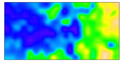
Figure 1: Locations of Acalypha, Lonchocarpus, and Capparis trees and image of interpolated potassium content in the surface soil (from top to bottom).

Figure 1 shows the spatial locations of three tree species, Acalypha diversifolia (528 trees), Lonchocarpus heptaphyllus (836 trees) and Capparis frondosa (3299 trees), in a $1000m\times 500m$ observation window on Barro Colorado Island Condit et al. (1996); Condit (1998); Hubbell and Foster (1983). Also one example of an environmental variable (potassium content in the soil) is shown.

In order to study the niche assembly hypothesis we use our quasi-likelihood method to fit log-linear regression models for the intensity functions depending on environmental variables. In addition to soil potassium content (K, divided by 1000), we consider nine other covariates for the intensity functions: pH, elevation (dem), slope gradient (grad), multi-resolution index of valley bottom flatness (mrvbf), incoming mean solar radiation (solar), topographic wetness index (twi) as well as soil contents of copper (Cu), mineralized nitrogen (Nmin) and phosphorus (P). The quasi-likelihood estimation was implemented as in the simulation study using a $100\times 50$ grid for the numerical quadrature and tapering tuning parameter $\epsilon=0.01$.

For each species we initially fit the following pair correlation functions of normal variance mixture type Jalilian et al. (2012):

$$g({\mathbf{r}};{\boldsymbol{\psi}})=1+c({\mathbf{r}};{\boldsymbol{\psi}}),\quad{\mathbf{r}}\in\mathbb{R}^{2},$$

where the covariance function $c({\mathbf{r}};{\boldsymbol{\psi}})$ is either Gaussian

$$c({\mathbf{r}};(\sigma^{2},\alpha))=\sigma^{2}\exp\big{[}-(\|{\mathbf{r}}\|/\alpha)^{2}\big{]},$$

Matérn ($K_{\nu}$ is the modified Bessel function of the second kind)

$$c({\mathbf{r}};(\sigma^{2},\alpha,\nu))=\sigma^{2}\frac{(\|{\mathbf{r}}\|/\alpha)^{\nu}K_{\nu}(\|{\mathbf{r}}\|/\alpha)}{2^{\nu-1}\Gamma(\nu)},$$

or Cauchy

$$c({\mathbf{r}};(\sigma^{2},\alpha))=\sigma^{2}\big{[}1+(\|{\mathbf{r}}\|/\alpha)^{2}\big{]}^{-3/2}.$$

These covariance functions represent very different tail behavior ranging from light (Gaussian), exponential (Matérn), to heavy tails (Cauchy). The pair correlation function obtained with the Gaussian covariance function is just a re-parametrization of the Thomas process pair correlation function (26). For the Matérn covariance we consider three different values of the shape parameter $\nu=0.25,0.5$ and $1$. With $\nu=0.5$ the exponential model $c[{\mathbf{r}};(\sigma^{2},\alpha,0.5)]=\sigma^{2}\exp(-\|{\mathbf{r}}\|/\alpha)$ is obtained while $\nu=0.25$ and $1$ yields respectively a log convex and a log concave covariance function.

Figure 2 shows $c(\cdot;\hat{\boldsymbol{\psi}})=g(\cdot;\hat{\boldsymbol{\psi}})-1$ for the best fitting (in terms of the minimum contrast criterion for the corresponding $K$-function) pair correlation functions: Cauchy for Acalypha ($\hat{\boldsymbol{\psi}}=(15.4,2.3)$), Matérn ($\hat{\boldsymbol{\psi}}=(2.2,15.5,0.5$)) for Lonchocarpus and Matérn ($\hat{\boldsymbol{\psi}}=(1.2,30.2,0.25)$) for Capparis.

Figure 2: Best fitting covariance functions $c(\cdot;\hat{\boldsymbol{\psi}})=g(\cdot;\hat{\boldsymbol{\psi}})-1$ for Acalypha (left), Lonchocarpus (middle), and Capparis (right).

The tapering distances corresponding to $\epsilon=0.01$ are respectively 20.9, 71.3 and 112.2 for the three species. Hence Capparis is the computationally most challenging case.

Backward model selection with significance level 5% was carried out for each species. According to the quasi-likelihood results, potassium (K) is a significant covariate at the 5% level for Acalypha, mineralized nitrogen (Nmin) and phosphorous (P) are significant for Lonchocarpus while elevation (dem), gradient (grad) and potassium are significant for Capparis. The fitted linear predictors with estimated standard errors in parenthesis are respectively -6.9+4.4K (0.085,1.2), -6.5-0.028Nmin-0.15P (0.088,0.0069,0.055) and -5.1+0.020dem-2.3grad+3.9K (0.078,0.0090,0.98,1.0).

The computing time for the QL estimation depends both on the grid used for the numerical quadrature and the tapering tuning parameter $\epsilon$. We also tried out a $150\times 75$ grid and $\epsilon=0.05$ and $0.02$ for the QL fitting of the final models. Parameter estimates and parameter estimation computing time (system plus CPU time on a 2.90 GHz lap top) for all combinations of grid sizes, $\epsilon$ and species are shown in Table 2. The computing time for the parameter estimation depends much on both grid sizes, $\epsilon$ and species (i.e. range of spatial dependence). Computing time including computation of standard errors is shown in Table 3, together with the computed standard errors for the parameter estimates in Table 2. The computing time with computation of standard errors is less sensitive to $\epsilon$ and species since in this case the main computational burden arises from the non-sparse matrix in (23). For the $100\times 50$ grid and $\epsilon=0.01$, the maximal computing time of 29.1 seconds (including computation of standard errors) occurs for Capparis. In contrast to large variations in the computing time, the parameter estimates and estimated standard errors for each species are very stable across the combinations of grid sizes and tapering parameter $\epsilon$.

Table 2: Computing times (T) in seconds (without computation of standard errors) and QL parameter estimates for different combinations of grid size and tapering.

		Acalypha		Lonchocarpus		Capparis
Grid	$\epsilon$	T	estm.	T	estm.	T	estm.
$100\!\!\times\!\!50$	0.05	0.3	-6.9 4.4	1.1	-6.5 -0.028 -0.16	2.4	-5.1 0.021 -2.4 4.2
	0.01	0.4	-6.9 4.4	2.6	-6.5 -0.028 -0.15	7.5	-5.1 0.020 -2.3 3.9
	.002	0.6	-6.9 4.4	4.4	-6.5 -0.028 -0.15	12.7	-5.1 0.020 -2.3 3.8
$150\!\!\times\!\!75$	0.05	0.5	-6.9 4.3	8.5	-6.5 -0.028 -0.16	34.9	-5.1 0.021 -2.3 4.1
	0.01	1.8	-6.9 4.3	23.7	-6.5 -0.028 -0.15	80.4	-5.1 0.020 -2.2 3.8
	.002	5.3	-6.9 4.3	41.6	-6.5 -0.028 -0.15	163.6	-5.1 0.020 -2.2 3.8

Table 3: Computing times (T) in seconds (including computation of standard errors) and estimated standard errors of QL parameter estimates for different combinations of grid size and tapering

		Acalypha		Lonchocarpus		Capparis
Grid	$\epsilon$	T	sd.	T	sd.	T	sd.
$100\!\!\times\!\!50$	0.05	12.1	0.085 1.2	22.4	0.088 0.0069 0.055	24.7	0.078 0.0091 0.98 1.1
	0.01	12.0	0.085 1.2	24.0	0.088 0.0069 0.055	29.1	0.078 0.0090 0.98 1.0
	.002	12.1	0.085 1.2	25.9	0.088 0.0069 0.055	34.3	0.078 0.0090 0.98 1.0
$150\!\!\times\!\!75$	0.05	59.4	0.079 1.1	187.2	0.087 0.0069 0.055	223.4	0.078 0.0090 0.96 1.0
	0.01	58.9	0.079 1.1	204.6	0.087 0.0069 0.055	255.2	0.078 0.0089 0.96 1.0
	.002	63.6	0.079 1.1	226.5	0.087 0.0069 0.055	300.9	0.078 0.0089 0.96 1.0

7 DISCUSSION

In contrast to maximum likelihood estimation our quasi-likelihood estimation method only requires the specification of the intensity function and a pair correlation function. Moreover, the estimation of the regression parameters can be expected to be quite robust toward misspecification of the pair correlation function since the resulting estimating equation is unbiased for any choice of pair correlation function. In the data example we considered pair correlation functions obtained from covariance functions of normal variance mixture type. Alternatively one might consider pair correlation functions of the log Gaussian Cox process type (Møller et al., 1998), i.e., $g({\mathbf{r}})=\exp\big{[}c({\mathbf{r}})\big{]}$, where $c(\cdot)$ is an arbitrary covariance function.

If a log Gaussian Cox process is deemed appropriate, a computationally feasible alternative to our approach is to use the method of integrated nested Laplace approximation (INLA, Rue et al., 2009; Illian et al., 2012) to implement Bayesian inference. However, in order to apply INLA it is required that the Gaussian field can be approximated well by a Gaussian Markov random field and this can limit the choice of covariance function. For example, the accurate Gaussian Markov random field approximations in Lindgren et al. (2011) of Gaussian fields with Matérn covariance functions are restricted to integer $\nu$ in the planar case. In contrast, our approach is not subject to such limitations and can also be applied to non-log Gaussian Cox processes.

We finally note that for the Nyström approximate solution of the Fredholm equation we used the simplest possible quadrature scheme given by a Riemann sum for a fine grid. This entails a minimum of assumptions regarding the integrand but at the expense of a typically high-dimensional covariance matrix ${\mathbf{V}}$. There may hence be scope for further development considering more sophisticated numerical quadrature schemes.
Acknowledgments
Abdollah Jalilian and Rasmus Waagepetersen’s research was supported by the Danish Natural Science Research Council, grant 09-072331 ‘Point process modeling and statistical inference’, Danish Council for Independent Research — Natural Sciences, Grant 12-124675, ‘Mathematical and Statistical Analysis of Spatial Data’, and by Centre for Stochastic Geometry and Advanced Bioimaging, funded by a grant from the Villum Foundation. Yongtao Guan’s research was supported by NSF grant DMS-0845368, by NIH grant 1R01DA029081-01A1 and by the VELUX Visiting Professor Programmme.

The BCI forest dynamics research project was made possible by National Science Foundation grants to Stephen P. Hubbell: DEB-0640386, DEB-0425651, DEB-0346488, DEB-0129874, DEB-00753102, DEB-9909347, DEB-9615226, DEB-9615226, DEB-9405933, DEB-9221033, DEB-9100058, DEB-8906869, DEB-8605042, DEB-8206992, DEB-7922197, support from the Center for Tropical Forest Science, the Smithsonian Tropical Research Institute, the John D. and Catherine T. MacArthur Foundation, the Mellon Foundation, the Celera Foundation, and numerous private individuals, and through the hard work of over 100 people from 10 countries over the past two decades. The plot project is part of the Center for Tropical Forest Science, a global network of large-scale demographic tree plots.

The BCI soils data set were collected and analyzed by J. Dalling, R. John, K. Harms, R. Stallard and J. Yavitt with support from NSF DEB021104, 021115, 0212284, 0212818 and OISE 0314581, STRI and CTFS. Paolo Segre and Juan Di Trani provided assistance in the field. The covariates dem, grad, mrvbf, solar and twi were computed in SAGA GIS by Tomislav Hengl (http://spatial-analyst.net/).

Appendix A Condition for optimality

To show that (8) implies non-negative definiteness of (7), let $\hat{\mathbf{e}}_{\boldsymbol{\phi}}({\boldsymbol{\beta}})={\mathbf{e}}_{\mathbf{f}}({\boldsymbol{\beta}}){\boldsymbol{\Sigma}}_{\mathbf{f}}^{-1}{\boldsymbol{\Sigma}}_{{\mathbf{f}}{\boldsymbol{\phi}}}$ be the optimal linear predictor of ${\mathbf{e}}_{\boldsymbol{\phi}}({\boldsymbol{\beta}})$ given ${\mathbf{e}}_{\mathbf{f}}({\boldsymbol{\beta}})$. Then

$${\mathbb{V}\mathrm{ar}}[\hat{\mathbf{e}}_{\boldsymbol{\phi}}({\boldsymbol{\beta}})-{\mathbf{e}}_{\boldsymbol{\phi}}({\boldsymbol{\beta}})]={\boldsymbol{\Sigma}}_{\boldsymbol{\phi}}-{\boldsymbol{\Sigma}}_{{\boldsymbol{\phi}}{\mathbf{f}}}{\boldsymbol{\Sigma}}^{-1}_{\mathbf{f}}{\boldsymbol{\Sigma}}_{{\mathbf{f}}{\boldsymbol{\phi}}}$$

is non-negative definite whereby

$${\mathbf{S}}_{\boldsymbol{\phi}}{\boldsymbol{\Sigma}}_{\boldsymbol{\phi}}^{-1}{\mathbf{S}}_{\boldsymbol{\phi}}-{\mathbf{S}}_{\boldsymbol{\phi}}{\boldsymbol{\Sigma}}_{\boldsymbol{\phi}}^{-1}{\boldsymbol{\Sigma}}_{{\boldsymbol{\phi}}{\mathbf{f}}}{\boldsymbol{\Sigma}}_{\mathbf{f}}^{-1}{\boldsymbol{\Sigma}}_{{\mathbf{f}}{\boldsymbol{\phi}}}{\boldsymbol{\Sigma}}_{{\boldsymbol{\phi}}}^{-1}{\mathbf{S}}_{\boldsymbol{\phi}}$$

is non-negative definite too. Hence, (7) is non-negative definite provided

$${\mathbf{S}}_{\boldsymbol{\phi}}{\boldsymbol{\Sigma}}_{\boldsymbol{\phi}}^{-1}{\boldsymbol{\Sigma}}_{{\boldsymbol{\phi}}{\mathbf{f}}}={\mathbf{S}}_{\mathbf{f}}$$

which follows from (8) (in particular, (8) implies ${\boldsymbol{\Sigma}}_{\boldsymbol{\phi}}={\boldsymbol{\Sigma}}_{{\boldsymbol{\phi}}{\boldsymbol{\phi}}}={\mathbf{S}}_{\boldsymbol{\phi}}$).

Appendix B SOLUTION USING NEUMANN SERIES EXPANSION

Suppose that $\|{\mathbf{T}}\|_{\text{op}}=\sup\{\|{\mathbf{T}}{\mathbf{f}}\|_{\infty}/\|{\mathbf{f}}\|_{\infty}\>:\>\|{\mathbf{f}}\|_{\infty}\neq 0\}<1$ where $\|{\mathbf{f}}\|_{\infty}$ denotes the supremum norm of a continuous function ${\mathbf{f}}$ on $W$. Then we can obtain the solution ${\boldsymbol{\phi}}$ of (10) using a Neumann series expansion which may provide additional insight on the properties of ${\boldsymbol{\phi}}$. More specifically,

$${\boldsymbol{\phi}}=\sum_{k=0}^{\infty}(-{\mathbf{T}})^{k}\frac{{\boldsymbol{\lambda}}^{\prime}}{\lambda}.$$ (24)

If the infinite sum in (24) is truncated to the first term ($k=0$) then (12) becomes the Poisson score. Note that

$$\|{\mathbf{T}}\|_{\infty}\leq\sup_{{\mathbf{u}}\in W}\int_{W}|t({\mathbf{u}},{\mathbf{v}})|\mathrm{d}{\mathbf{v}}.$$

Hence, a sufficient condition for the validity of the Neumann series expansion is

$$\sup_{{\mathbf{u}}\in W}\lambda({\mathbf{u}};{\boldsymbol{\beta}})\int_{\mathbb{R}^{2}}\big{|}g({\mathbf{r}})-1\big{|}\mathrm{d}{\mathbf{r}}<1.$$ (25)

Condition (25) roughly requires that $g({\mathbf{r}})-1$ does not decrease too slowly to zero and/or that $\lambda$ is moderate. For example, suppose that $g$ is the pair correlation function of a Thomas cluster process (e.g. Møller and Waagepetersen, 2004, Chapter 5),

$$g({\mathbf{r}})-1=\exp\big{[}-\|{\mathbf{r}}\|^{2}/(4\omega^{2})\big{]}/(4\pi\omega^{2}\kappa),\;\hbox{ for some }\kappa,\omega>0,$$ (26)

where $\kappa$ is the intensity of the parent process and $\omega$ is the normal dispersal parameter. Then,

$$\int_{\mathbb{R}^{2}}\big{|}g({\mathbf{r}})-1\big{|}\mathrm{d}{\mathbf{r}}=\frac{1}{4\pi\kappa\omega^{2}}\int_{\mathbb{R}^{2}}\exp(-\frac{\|{\mathbf{r}}\|^{2}}{4\omega^{2}})\mathrm{d}{\mathbf{r}}=1/\kappa$$

and (25) is equivalent to $\sup_{{\mathbf{u}}\in W}\lambda({\mathbf{u}};{\boldsymbol{\beta}})<\kappa.$ In this case, Condition (25) can be quite restrictive. However, the Neumann series expansion is not essential for our approach and we use it only for checking the conditions for asymptotic results; see Appendix C.

Appendix C CONDITIONS AND LEMMAS

To verify the existence of a $|W_{n}|^{1/2}$ consistent sequence of solutions $\hat{\boldsymbol{\beta}}_{n}$, we assume that the following conditions are satisfied:

1. $\lambda({\mathbf{u}};{\boldsymbol{\beta}})=\lambda({\mathbf{z}}({\mathbf{u}}){\boldsymbol{\beta}}^{\mbox{\scriptsize\sf T}})$ where $\lambda(\cdot)>0$ is twice continuously differentiable and
   $\sup_{{\mathbf{u}}\in\mathbb{R}^{2}}\|{\mathbf{z}}({\mathbf{u}})\|<K_{1}$ for some $K_{1}<\infty$.

2. for some $0<K_{2}<\infty$, $\int_{\mathbb{R}^{2}}\big{|}g({\mathbf{r}};{\boldsymbol{\psi}}^{*})-1\big{|}\mathrm{d}{\mathbf{r}}\leq K_{2}$.

3. ${\boldsymbol{\phi}}_{n,{\boldsymbol{\theta}}}({\mathbf{u}},{\boldsymbol{\beta}})$ is differentiable with respect to ${\boldsymbol{\theta}}$ and ${\boldsymbol{\beta}}$, and for $|{\boldsymbol{\phi}}_{n,{\boldsymbol{\theta}}}({\mathbf{u}},{\boldsymbol{\beta}})|$, $|\mathrm{d}{\boldsymbol{\phi}}_{n,{\boldsymbol{\theta}}}({\mathbf{u}},{\boldsymbol{\beta}})/\mathrm{d}{\boldsymbol{\beta}}|$ and $|\mathrm{d}{\boldsymbol{\phi}}_{n,{\boldsymbol{\theta}}}({\mathbf{u}},{\boldsymbol{\beta}})/\mathrm{d}{\boldsymbol{\theta}}|$, the supremum over ${\mathbf{u}}\in\mathbb{R}^{2},{\boldsymbol{\beta}}\in b({\boldsymbol{\beta}}^{*},K_{3}),{\boldsymbol{\theta}}\in b({\boldsymbol{\theta}}^{*},K_{3})$ is bounded for some $K_{3}>0$, where $b(\mathbf{x},r)$ denotes the ball centered at $\mathbf{x}$ with radius $r>0$.

4. $|W_{n}|^{1/2}(\tilde{\boldsymbol{\theta}}_{n}-{\boldsymbol{\theta}}^{*})$ is bounded in probability.

5. $l=\liminf_{n}l_{n}>0$, where for each $n$, $l_{n}$ denotes the minimal eigenvalue of

   $$\bar{\mathbf{S}}_{n,{\boldsymbol{\theta}}^{*}}({\boldsymbol{\beta}}^{*})=|W_{n}|^{-1}{\mathbb{E}}{\mathbf{J}}_{n,{\boldsymbol{\theta}}^{*}}({\boldsymbol{\beta}}^{*})=|W_{n}|^{-1}\int_{W_{n}}{\boldsymbol{\phi}}_{n,{\boldsymbol{\theta}}^{*}}({\mathbf{u}})^{\mbox{\scriptsize\sf T}}{\boldsymbol{\lambda}}^{\prime}({\mathbf{u}};{\boldsymbol{\beta}}^{*})\mathrm{d}{\mathbf{u}}.$$

Condition C1 and C2 imply L1 and L2 below.

1. for $\lambda({\mathbf{u}};{\boldsymbol{\beta}})$, ${\boldsymbol{\lambda}}^{\prime}({\mathbf{u}};{\boldsymbol{\beta}})$ and ${\boldsymbol{\lambda}}^{\prime\prime}({\mathbf{u}};{\boldsymbol{\beta}})$, the supremum over ${\mathbf{u}}\in\mathbb{R}^{2},{\boldsymbol{\beta}}\in b({\boldsymbol{\beta}}^{*},K_{3}),{\boldsymbol{\theta}}\in b({\boldsymbol{\theta}}^{*},K_{3})$ is bounded.

2. for a function $h:\mathbb{R}^{2}\to\mathbb{R}$,

   $${\mathbb{V}\mathrm{ar}}\sum_{{\mathbf{u}}\in X\cap W_{n}}h({\mathbf{u}})\leq|W_{n}|\big{[}1+\sup_{{\mathbf{u}}\in W_{n}}\lambda({\mathbf{u}};{\boldsymbol{\beta}}^{*})K_{2}\big{]}\sup_{{\mathbf{u}}\in W_{n}}h({\mathbf{u}})^{2}\sup_{{\mathbf{u}}\in W_{n}}\lambda({\mathbf{u}};{\boldsymbol{\beta}}^{*}).$$

   In particular, $|W_{n}|^{-1}{\mathbb{V}\mathrm{ar}}\sum_{{\mathbf{u}}\in X\cap W_{n}}h({\mathbf{u}})$ is bounded when $h$ is bounded.

The condition C3 is not so easy to verify in general due to the abstract nature of the function ${\boldsymbol{\phi}}_{n,{\boldsymbol{\theta}}}$. However, it can be verified e.g. assuming that ${\boldsymbol{\phi}}_{n,{\boldsymbol{\theta}}}$ can be expressed using the Neumann series. Condition C4 holds under conditions specified in Waagepetersen and Guan (2009) (including e.g. C1 and C2). Condition C5 is not unreasonable since

$$\bar{\mathbf{S}}_{n,{\boldsymbol{\theta}}^{*}}({\boldsymbol{\beta}}^{*})=|W_{n}|^{-1}\int_{W_{n}}\Big{[}\frac{{\boldsymbol{\lambda}}^{\prime}({\mathbf{u}};{\boldsymbol{\beta}}^{*})}{\lambda({\mathbf{u}};{\boldsymbol{\beta}}^{*})^{1/2}}\Big{]}^{\mbox{\scriptsize\sf T}}\Big{[}({\mathbf{I}}+{\mathbf{T}}^{s}_{n,{\boldsymbol{\theta}}^{*}})^{-1}\frac{{\boldsymbol{\lambda}}^{\prime}(\cdot;{\boldsymbol{\beta}}^{*})}{\lambda(\cdot;{\boldsymbol{\beta}}^{*})^{1/2}}\Big{]}({\mathbf{u}})\mathrm{d}{\mathbf{u}}$$

and $({\mathbf{I}}+{\mathbf{T}}^{s}_{n,{\boldsymbol{\theta}}^{*}})^{-1}$ is a positive operator (see Section 3.1). Since $\bar{\boldsymbol{\Sigma}}_{n}=\bar{\mathbf{S}}_{n,{\boldsymbol{\theta}}^{*}}({\boldsymbol{\beta}}^{*})$, C5 also implies

1. $l=\liminf_{n}l_{n}>0$ where for each $n$, $l_{n}$ denotes the minimal eigenvalue of $\bar{\boldsymbol{\Sigma}}_{n}$.

To prove the asymptotic normality of $|W_{n}|^{-1/2}{\mathbf{e}}_{n,\tilde{\boldsymbol{\theta}}_{n}}({\boldsymbol{\beta}}^{*})\bar{\boldsymbol{\Sigma}}_{n}^{-1/2}$, we assume that the following additional conditions are satisfied:

1. $W_{n}=nA$ where $A\subset(0,1]\times(0,1]$ is the interior of a simple closed curve with nonempty interior.

2. $\sup_{p}{\alpha(p;k)\over p}=\hbox{O}(k^{-\epsilon})$ for some $\epsilon>2$, where $\alpha(p;k)$ is the strong mixing coefficient (Rosenblatt, 1956). For each $p$ and $k$, the mixing condition measures the dependence between $X\cap E_{1}$ and $X\cap E_{2}$ where $E_{1}$ and $E_{2}$ are arbitrary Borel subsets of $\mathbb{R}^{2}$ each of volume less than $p$ and at distance $k$ apart.

3. for some $K_{4}<\infty$ and $k=3,4$,

   $$\sup_{{\mathbf{u}}_{1}\in\mathbb{R}^{2}}\int_{\mathbb{R}^{2}}\cdots\int_{\mathbb{R}^{2}}\big{|}Q_{k}({\mathbf{u}}_{1},\cdots,{\mathbf{u}}_{k})\big{|}\mathrm{d}{\mathbf{u}}_{2}\cdots\mathrm{d}{\mathbf{u}}_{k}<K_{4},$$

   where $Q_{k}$ is the $k$-th order cumulant density function of $X$ (e.g. Guan and Loh, 2007).

Conditions N1-N3 correspond to conditions (2), (3) and (6), respectively, in Guan and Loh (2007). See this paper for a discussion of the conditions.

Appendix D EXISTENCE OF A $|W_{n}|^{1/2}$ CONSISTENT $\hat{\boldsymbol{\beta}}_{n}$

We use Theorem 2 and Remark 1 in Waagepetersen and Guan (2009) to show the existence of a $|W_{n}|^{1/2}$ consistent sequence of solutions $\hat{\boldsymbol{\beta}}_{n}$. Let $\|{\mathbf{A}}\|_{M}=\sup_{ij}|a_{ij}|$ for a matrix ${\mathbf{A}}=[a_{ij}]_{ij}$. With ${\mathbf{V}}_{n}=|W_{n}|^{1/2}\bar{\boldsymbol{\Sigma}}_{n}^{1/2}$ we need to verify the following results:

1. $\|{\mathbf{V}}_{n}^{-1}\|_{M}\rightarrow 0.$

2. For any $d>0$,

   $$\sup_{{\boldsymbol{\beta}}:\|({\boldsymbol{\beta}}-{\boldsymbol{\beta}}^{*}){\mathbf{V}}_{n}\|\leq d}\|{\mathbf{V}}_{n}^{-1}\big{[}{\mathbf{J}}_{n,\tilde{\boldsymbol{\theta}}_{n}}({\boldsymbol{\beta}})-{\mathbf{J}}_{n,\tilde{\boldsymbol{\theta}}_{n}}({\boldsymbol{\beta}}^{*})\big{]}{\mathbf{V}}_{n}^{-1}\|_{M}$$

   converges to zero in probability.

3. $\|{\mathbf{J}}_{n,\tilde{\boldsymbol{\theta}}_{n}}({\boldsymbol{\beta}}^{*})/|W_{n}|-\bar{\mathbf{S}}_{n,{\boldsymbol{\theta}}^{*}}({\boldsymbol{\beta}}^{*})\|_{M}$ converges to zero in probability.

4. ${\mathbf{e}}_{n,\tilde{\boldsymbol{\theta}}_{n}}({\boldsymbol{\beta}}^{*}){\mathbf{V}}_{n}^{-1}$ is bounded in probability.

5. $\liminf_{n}l_{n}>0$ where

   $$l_{n}=\inf_{\|{\mathbf{x}}\|=1}{\mathbf{x}}\bar{\boldsymbol{\Sigma}}_{n}^{-1/2}\bar{\mathbf{S}}_{n,{\boldsymbol{\theta}}^{*}}({\boldsymbol{\beta}}^{*})\bar{\boldsymbol{\Sigma}}_{n}^{-1/2}{\mathbf{x}}^{\mbox{\scriptsize\sf T}}.$$

We now demonstrate that R1-R5 hold under the conditions C1-C5 listed in Appendix C. For each of the results below the required conditions or previous results are indicated in square brackets.
R1 [C3, L1-L3]: By C3, L1 and L2 the entries in $\bar{\boldsymbol{\Sigma}}_{n}$ are bounded from below and above. Moreover, by L3 the determinant of $\bar{\boldsymbol{\Sigma}}_{n}$ is bounded below by $l^{p}>0$.
R2 [R1, C3, L1, L2, C4]: We show that

$$\sup_{({\boldsymbol{\theta}},{\boldsymbol{\beta}}):\|({\boldsymbol{\theta}}-{\boldsymbol{\theta}}^{*},{\boldsymbol{\beta}}-{\boldsymbol{\beta}}^{*})|W_{n}|^{1/2}\|\leq d}\||W_{n}|^{-1}\big{[}{\mathbf{J}}_{n,{\boldsymbol{\theta}}}({\boldsymbol{\beta}})-{\mathbf{J}}_{n,{\boldsymbol{\theta}}^{*}}({\boldsymbol{\beta}}^{*})\big{]}\|_{M}$$

converges to zero in probability. Note

$$|W_{n}|^{-1}{\mathbf{J}}_{n,{\boldsymbol{\theta}}}({\boldsymbol{\beta}})={\mathbf{L}}_{n,{\boldsymbol{\theta}}}({\boldsymbol{\beta}})+{\mathbf{M}}_{n,{\boldsymbol{\theta}}}({\boldsymbol{\beta}})$$

where

$${\mathbf{L}}_{n,{\boldsymbol{\theta}}}({\boldsymbol{\beta}})=-\sum_{{\mathbf{u}}\in X}{\mathbf{f}}_{1,n,{\boldsymbol{\theta}}}({\mathbf{u}},{\boldsymbol{\beta}})\text{ and }{\mathbf{M}}_{n,{\boldsymbol{\theta}}}({\boldsymbol{\beta}})=\int_{\mathbb{R}^{2}}{\mathbf{f}}_{2,n,{\boldsymbol{\theta}}}({\mathbf{u}},{\boldsymbol{\beta}})$$

with

$${\mathbf{f}}_{1,n,{\boldsymbol{\theta}}}({\mathbf{u}},{\boldsymbol{\beta}})=\frac{1[{\mathbf{u}}\in W_{n}]}{|W_{n}|}\frac{\mathrm{d}}{\mathrm{d}{\boldsymbol{\beta}}^{\mbox{\scriptsize\sf T}}}{\boldsymbol{\phi}}_{n,{\boldsymbol{\theta}}}({\mathbf{u}},{\boldsymbol{\beta}})$$

and

$${\mathbf{f}}_{2,n,{\boldsymbol{\theta}}}({\mathbf{u}},{\boldsymbol{\beta}})=\frac{1[{\mathbf{u}}\in W_{n}]}{|W_{n}|}\big{[}\lambda({\mathbf{u}};{\boldsymbol{\beta}})\frac{\mathrm{d}}{\mathrm{d}{\boldsymbol{\beta}}^{\mbox{\scriptsize\sf T}}}{\boldsymbol{\phi}}_{n,{\boldsymbol{\theta}}}({\mathbf{u}},{\boldsymbol{\beta}})+{\boldsymbol{\lambda}}^{\prime}({\mathbf{u}};{\boldsymbol{\beta}})^{\mbox{\scriptsize\sf T}}{\boldsymbol{\phi}}_{n,{\boldsymbol{\theta}}}({\mathbf{u}},{\boldsymbol{\beta}})\big{]}.$$

Define

$$h_{i,n}({\mathbf{u}})=\sup_{({\boldsymbol{\theta}},{\boldsymbol{\beta}}):\|({\boldsymbol{\theta}}-{\boldsymbol{\theta}}^{*},{\boldsymbol{\beta}}-{\boldsymbol{\beta}}^{*})|W_{n}|^{1/2}\|\leq d}|{\mathbf{f}}_{i,n,{\boldsymbol{\theta}}}({\mathbf{u}},{\boldsymbol{\beta}})-{\mathbf{f}}_{i,n,{\boldsymbol{\theta}}^{*}}({\mathbf{u}},{\boldsymbol{\beta}}^{*})|,\,i=1,2$$

and note that $h_{i,n}({\mathbf{u}})$ converge to zero as $n\rightarrow\infty$. Then

$$\sup_{({\boldsymbol{\theta}},{\boldsymbol{\beta}}):\|({\boldsymbol{\theta}}-{\boldsymbol{\theta}}^{*},{\boldsymbol{\beta}}-{\boldsymbol{\beta}}^{*})|W_{n}|^{1/2}\|\leq d}|{\mathbf{M}}_{n,{\boldsymbol{\theta}}}({\boldsymbol{\beta}})-{\mathbf{M}}_{n,{\boldsymbol{\theta}}^{*}}({\boldsymbol{\beta}}^{*})|\leq\int_{\mathbb{R}^{2}}h_{1,n}({\mathbf{u}})\mathrm{d}{\mathbf{u}}$$

where the right hand side converges to zero by dominated convergence. Moreover,

$$\sup_{({\boldsymbol{\theta}},{\boldsymbol{\beta}}):\|({\boldsymbol{\theta}}-{\boldsymbol{\theta}}^{*},{\boldsymbol{\beta}}-{\boldsymbol{\beta}}^{*})|W_{n}|^{1/2}\|\leq d}\big{|}{\mathbf{L}}_{n,{\boldsymbol{\theta}}}({\boldsymbol{\beta}})-{\mathbf{L}}_{n,{\boldsymbol{\theta}}^{*}}({\boldsymbol{\beta}}^{*})\big{|}\leq\sum_{{\mathbf{u}}\in X}h_{2,n}({\mathbf{u}})\leq\\ \Big{|}\sum_{{\mathbf{u}}\in X}h_{2,n}({\mathbf{u}})-{\mathbb{E}}\sum_{{\mathbf{u}}\in X}h_{2,n}({\mathbf{u}})\Big{|}+\Big{|}{\mathbb{E}}\sum_{{\mathbf{u}}\in X}h_{2,n}({\mathbf{u}})\Big{|}.$$

The first term on the right hand side converges to zero in probability by Chebyshev’s inequality and the second term converges to zero by dominated convergence.
R3 [R1, L1, L2, C4]:

$$|W_{n}|^{-1}{\mathbf{J}}_{n,\tilde{\boldsymbol{\theta}}_{n}}({\boldsymbol{\beta}}^{*})-\bar{\mathbf{S}}_{n}({\boldsymbol{\beta}}^{*})=\\ |W_{n}|^{-1}\big{[}{\mathbf{J}}_{n,\tilde{\boldsymbol{\theta}}_{n}}({\boldsymbol{\beta}}^{*})-{\mathbf{J}}_{n,{\boldsymbol{\theta}}^{*}}({\boldsymbol{\beta}}^{*})\big{]}+\big{[}|W_{n}|^{-1}{\mathbf{J}}_{n,{\boldsymbol{\theta}}^{*}}({\boldsymbol{\beta}}^{*})-\bar{\mathbf{S}}_{n}({\boldsymbol{\beta}}^{*})\big{]}$$

It follows from the proof of R2 that the first term on the right hand side converges to zero in probability. The last term converges to zero in probability by Chebyshev’s inequality.
R4 [C3, L1, L2, C4]: Since ${\mathbb{V}\mathrm{ar}}{\mathbf{e}}_{n,{\boldsymbol{\theta}}^{*}}({\boldsymbol{\beta}}^{*}){\mathbf{V}}_{n}^{-1}$ is the identity matrix, ${\mathbf{e}}_{n,{\boldsymbol{\theta}}^{*}}({\boldsymbol{\beta}}^{*}){\mathbf{V}}_{n}^{-1}$ is bounded in probability by Chebyshev’s inequality. The result then follows by showing that
$|W_{n}|^{-1/2}\big{[}{\mathbf{e}}_{n,\tilde{\boldsymbol{\theta}}_{n}}({\boldsymbol{\beta}}^{*})-{\mathbf{e}}_{n,{\boldsymbol{\theta}}^{*}}({\boldsymbol{\beta}}^{*})\big{]}$ converges to zero in probability. Let

$${\mathbf{f}}_{n}({\boldsymbol{\theta}})=|W_{n}|^{-1}\frac{\mathrm{d}}{\mathrm{d}{\boldsymbol{\theta}}^{\mbox{\scriptsize\sf T}}}{\mathbf{e}}_{n,{\boldsymbol{\theta}}}({\boldsymbol{\beta}}^{*})=\\ |W_{n}|^{-1}\Big{[}\sum_{{\mathbf{u}}\in X\cap W_{n}}\frac{\mathrm{d}}{\mathrm{d}{\boldsymbol{\theta}}^{\mbox{\scriptsize\sf T}}}{\boldsymbol{\phi}}_{n,{\boldsymbol{\theta}}}({\mathbf{u}},{\boldsymbol{\beta}}^{*})-\int_{W_{n}}\lambda({\mathbf{u}};{\boldsymbol{\beta}}^{*})\frac{\mathrm{d}}{\mathrm{d}{\boldsymbol{\theta}}^{\mbox{\scriptsize\sf T}}}{\boldsymbol{\phi}}_{n,{\boldsymbol{\theta}}}({\mathbf{u}},{\boldsymbol{\beta}}^{*})\mathrm{d}{\mathbf{u}}\Big{]}.$$

Then

$$|W_{n}|^{-1/2}\big{[}{\mathbf{e}}_{n,\tilde{\boldsymbol{\theta}}_{n}}({\boldsymbol{\beta}}^{*})-{\mathbf{e}}_{n,{\boldsymbol{\theta}}^{*}}({\boldsymbol{\beta}}^{*})\big{]}=|W_{n}|^{1/2}(\tilde{\boldsymbol{\theta}}_{n}-{\boldsymbol{\theta}}^{*}){\mathbf{f}}_{n}(\mathbf{t}_{n})$$

where $\|\mathbf{t}_{n}-{\boldsymbol{\theta}}^{*}\|\leq\|\tilde{\boldsymbol{\theta}}_{n}-{\boldsymbol{\theta}}^{*}\|$ and the factor $|W_{n}|^{1/2}(\tilde{\boldsymbol{\theta}}_{n}-{\boldsymbol{\theta}}^{*})$ is bounded in probability. Further,

$${\mathbf{f}}_{n}(\mathbf{t}_{n})={\mathbf{f}}_{n}(\mathbf{t}_{n})-{\mathbf{f}}_{n}({\boldsymbol{\theta}}^{*})+{\mathbf{f}}_{n}({\boldsymbol{\theta}}^{*})$$

where ${\mathbf{f}}_{n}({\boldsymbol{\theta}}^{*})$ converges to zero in probability by Chebyshev’s inequality and ${\mathbf{f}}_{n}(\mathbf{t}_{n})-{\mathbf{f}}_{n}({\boldsymbol{\theta}}^{*})$ converges to zero in probability along the lines of the proof of R2.
R5 [C5, L3]: Follows directly from C5 and L3.

Appendix E ASYMPTOTIC NORMALITY OF $|W_{n}|^{-1/2}{\mathbf{e}}_{n,\tilde{\boldsymbol{\theta}}_{n}}({\boldsymbol{\beta}}^{*}){\boldsymbol{\Sigma}}_{n}^{-1/2}$

By the proof of R4 it suffices to show that $|W_{n}|^{-1/2}{\mathbf{e}}_{n,{\boldsymbol{\theta}}^{*}}({\boldsymbol{\beta}}^{*})\bar{\boldsymbol{\Sigma}}_{n}^{-1/2}$ is asymptotically normal. To do so we use the blocking technique used in Guan and Loh (2007). Specifically, Condition N1 implies that there is a sequence of windows $W_{n}^{B}=\cup_{i=1}^{k_{n}}W_{n}^{i}$ given for each $n$ by a union of $m_{n}\times m_{n}$ sub squares $W_{n}^{i}$, $i=1,\cdots,k_{n}$, such that $|W_{n}^{B}|/|W_{n}|\to 1$, $m_{n}=\hbox{O}(n^{\alpha})$ and the inter-distance between any two neighboring sub squares is of order $n^{\eta}$ for some $4/(2+\epsilon)<\eta<\alpha<1$. Let

$${\mathbf{e}}_{n,{\boldsymbol{\theta}}^{*}}^{B}({\boldsymbol{\beta}})=\sum_{{\mathbf{u}}\in X\cap W_{n}^{B}}{\boldsymbol{\phi}}_{n,{\boldsymbol{\theta}}^{*}}({\mathbf{u}};{\boldsymbol{\beta}})-\int_{W_{n}^{B}}{\boldsymbol{\phi}}_{n,{\boldsymbol{\theta}}^{*}}({\mathbf{u}};{\boldsymbol{\beta}})\lambda({\mathbf{u}};{\boldsymbol{\beta}})\mathrm{d}{\mathbf{u}}\equiv\sum_{i=1}^{k_{n}}{\mathbf{e}}_{n,{\boldsymbol{\theta}}^{*}}^{B,i}({\boldsymbol{\beta}}),$$

where

$${\mathbf{e}}_{n,{\boldsymbol{\theta}}^{*}}^{B,i}({\boldsymbol{\beta}})=\sum_{{\mathbf{u}}\in X\cap W_{n}^{i}}{\boldsymbol{\phi}}_{n,\theta^{*}}({\mathbf{u}};{\boldsymbol{\beta}})-\int_{W_{n}^{i}}{\boldsymbol{\phi}}_{n,{\boldsymbol{\theta}}^{*}}({\mathbf{u}};{\boldsymbol{\beta}})\lambda({\mathbf{u}};{\boldsymbol{\beta}})\mathrm{d}{\mathbf{u}}.$$

Define

$$\tilde{\mathbf{e}}_{n,{\boldsymbol{\theta}}^{*}}^{B}({\boldsymbol{\beta}})=\sum_{i=1}^{k_{n}}\tilde{\mathbf{e}}_{n,{\boldsymbol{\theta}}^{*}}^{B,i}({\boldsymbol{\beta}}),$$

where the $\tilde{\mathbf{e}}_{n,{\boldsymbol{\theta}}^{*}}^{B,i}({\boldsymbol{\beta}})$’s are independent and for each $i$ and $n$, $\tilde{\mathbf{e}}_{n,{\boldsymbol{\theta}}^{*}}^{B,i}({\boldsymbol{\beta}})$ is distributed as ${\mathbf{e}}_{n,{\boldsymbol{\theta}}^{*}}^{B,i}({\boldsymbol{\beta}})$. Let $\bar{\boldsymbol{\Sigma}}^{B}_{n}=|W_{n}^{B}|^{-1}{\mathbb{V}\mathrm{ar}}{\mathbf{e}}_{n,{\boldsymbol{\theta}}^{*}}^{B}({\boldsymbol{\beta}}^{*})$ and $\tilde{\boldsymbol{\Sigma}}_{n}^{B}=|W_{n}^{B}|^{-1}{\mathbb{V}\mathrm{ar}}\tilde{\mathbf{e}}_{n,{\boldsymbol{\theta}}^{*}}^{B}({\boldsymbol{\beta}}^{*})$. We need to verify the following results:

1. $||\tilde{\boldsymbol{\Sigma}}_{n}^{B}-\bar{\boldsymbol{\Sigma}}^{B}_{n}||_{M}\to 0$ and $||\bar{\boldsymbol{\Sigma}}_{n}^{B}-\bar{\boldsymbol{\Sigma}}_{n}||_{M}\to 0$ as $n\to\infty$,

2. $|W_{n}^{B}|^{-1/2}\tilde{\mathbf{e}}_{n,\theta^{*}}^{B}({\boldsymbol{\beta}}^{*})\left(\tilde{\boldsymbol{\Sigma}}_{n}^{B}\right)^{-1/2}$ is asymptotically standard normal,

3. $|W_{n}^{B}|^{-1/2}{\mathbf{e}}_{n,{\boldsymbol{\theta}}^{*}}^{B}({\boldsymbol{\beta}}^{*})\left(\tilde{\boldsymbol{\Sigma}}_{n}^{B}\right)^{-1/2}$ has the same asymptotic distribution as
   $|W_{n}^{B}|^{-1/2}\tilde{\mathbf{e}}_{n,{\boldsymbol{\theta}}^{*}}^{B}({\boldsymbol{\beta}}^{*})\left(\bar{\boldsymbol{\Sigma}}_{n}^{B}\right)^{-1/2}$,

4. $\||W_{n}^{B}|^{-1/2}{\mathbf{e}}_{n,{\boldsymbol{\theta}}^{*}}^{B}({\boldsymbol{\beta}}^{*})-|W_{n}|^{-1/2}{\mathbf{e}}_{n,{\boldsymbol{\theta}}^{*}}({\boldsymbol{\beta}}^{*})\|$ converges to zero in probability.

S1 [C2, C3, N1]: This follows from the proof of Theorem 2 in Guan and Loh (2007).
S2 [C2, C3, N3]: Conditions C2, C3 and N3 imply ${\mathbb{E}}[\tilde{\mathbf{e}}_{n,{\boldsymbol{\theta}}^{*}}^{i}({\boldsymbol{\beta}})^{4}]$ is bounded (see the proof of Lemma 1 in Guan and Loh, 2007). Thus, S2 follows from an application of Lyapunov’s central limit theorem.
S3 [N2]: this follows by bounding the difference between the characteristic functions of $|W_{n}^{B}|^{-1/2}{\mathbf{e}}_{n,{\boldsymbol{\theta}}^{*}}^{B}({\boldsymbol{\beta}}^{*})$ and $|W_{n}^{B}|^{-1/2}\tilde{\mathbf{e}}_{n,{\boldsymbol{\theta}}^{*}}^{B}({\boldsymbol{\beta}}^{*})$ using techniques in Ibramigov and Linnik (1971) and secondly applying the mixing condition N2, see also Guan et al. (2004).
S4 [C1-C3, C5, N1]: Recall that $|W_{n}^{B}|/|W_{n}|\to 1$ due to N1. By C5 we only need to show ${\mathbb{V}\mathrm{ar}}\big{[}{\mathbf{e}}_{n,\theta^{*}}({\boldsymbol{\beta}}^{*})-{\mathbf{e}}_{n,{\boldsymbol{\theta}}^{*}}^{B}({\boldsymbol{\beta}}^{*})\big{]}/|W_{n}|\to 0$. This is implied by conditions C1-C3 and $|W_{n}^{B}|/|W_{n}|\to 1$.

References

• Condit (1998) Condit, R. (1998). Tropical Forest Census Plots. Berlin, Germany and Georgetown, Texas: Springer-Verlag and R. G. Landes Company.
• Condit et al. (1996) Condit, R., S. P. Hubbell, and R. B. Foster (1996). Changes in tree species abundance in a neotropical forest: impact of climate change. Journal of Tropical Ecology 12, 231–256.
• Furrer et al. (2006) Furrer, R., M. G. Genton, and D. Nychka (2006). Covariance tapering for interpolation of large spatial datasets. Journal of Computational and Graphical Statistics 15, 502–523.
• Gotway and Stroup (1997) Gotway, C. A. and W. W. Stroup (1997). A generalized linear model approach to spatial data analysis and prediction. Journal of Agricultural, Biological, and Environmental Statistics 2, 157–178.
• Gray (2003) Gray, Robert, J. (2003). Weighted estimating equations for linear regression analysis of clustered failure time data. Lifetime Data Analysis 9(2), 123–138.
• Guan and Loh (2007) Guan, Y. and J. M. Loh (2007). A thinned block bootstrap procedure for modeling inhomogeneous spatial point patterns. Journal of the American Statistical Association 102, 1377–1386.
• Guan and Shen (2010) Guan, Y. and Y. Shen (2010). A weighted estimating estimation approach for inhomogeneous spatial point processes. Biometrika 97, 867–880.
• Guan et al. (2004) Guan, Y., M. Sherman, and J. A. Calvin (2004). A nonparametric test for spatial isotropy using subsampling. Journal of the American Statistical Society 99, 810–821.
• Hackbusch (1995) Hackbusch, W. (1995). Integral equations - theory and numerical treatment. Birkhäuser.
• Heyde (1997) Heyde, C. C. (1997). Quasi-likelihood and its application - a general approach to optimal parameter estimation. Springer Series in Statistics. Springer.
• Hubbell and Foster (1983) Hubbell, S. P. and R. B. Foster (1983). Diversity of canopy trees in a neotropical forest and implications for conservation. In S. L. Sutton, T. C. Whitmore, and A. C. Chadwick (Eds.), Tropical Rain Forest: Ecology and Management, pp.  25–41. Oxford: Blackwell Scientific Publications.
• Ibramigov and Linnik (1971) Ibramigov, I. A. and Y. V. Linnik (1971). Independent and stationary sequences of random variables. Groningen: Wolters-Noordhoff.
• Illian et al. (2012) Illian, J. B., S. H. Sørbye, and H. Rue (2012). A toolbox for fitting complex spatial point process models using integrated nested Laplace approximation (INLA). Annals of Applied Statistics 6, 1499–1530.
• Jalilian et al. (2012) Jalilian, A., Y. Guan, and R. Waagepetersen (2012). Decomposition of variance for spatial Cox processes. Scandinavian Journal of Statistics. Appeared online.
• Lax (2002) Lax, P. D. (2002). Functional analysis. Wiley.
• Liang and Zeger (1986) Liang, K. and S. L. Zeger (1986). Longitudinal data analysis using generalized linear models. Biometrika 73, 13–22.
• Lin and Clayton (2005) Lin, P.-S. and M. K. Clayton (2005). Analysis of binary spatial data by quasi-likelihood estimating equations. Annals of Statistics 33, 542–555.
• Lin et al. (2011) Lin, Y.-C., L.-W. Chang, K.-C. Yang, H.-H. Wang, and I.-F. Sun (2011). Point patterns of tree distribution determined by habitat heterogeneity and dispersal limitation. Oecologia 165, 175–184.
• Lindgren et al. (2011) Lindgren, F., H. Rue, and J. Lindström (2011). An explicit link between Gaussian fields and Gaussian Markov random fields: the stochastic partial differential equation approach. Journal of the Royal Statistical Society B 73, 423–498.
• Møller et al. (1998) Møller, J., A. R. Syversveen, and R. P. Waagepetersen (1998). Log Gaussian Cox processes. Scandinavian Journal of Statistics 25, 451–482.
• Møller and Waagepetersen (2004) Møller, J. and R. P. Waagepetersen (2004). Statistical inference and simulation for spatial point processes. Boca Raton: Chapman and Hall/CRC.
• Møller and Waagepetersen (2007) Møller, J. and R. P. Waagepetersen (2007). Modern statistics for spatial point processes. Scandinavian Journal of Statistics 34, 643–684.