Statefinder hierarchy of bimetric and galileon models for concordance cosmology

Abstract

In this paper, we use Statefinder hierarchy method to distinguish between bimetric theory of massive gravity, galileon modified gravity and DGP models applied to late time expansion of the universe. We also carry out comparison between bimetric and DGP models using Statefinder pairs $\{r,s\}$ and $\{r,q\}$. We show that statefinder diagnostic can differentiate between $\Lambda$CDM and above mentioned cosmological models of dark energy, and finally show that Statefinder $S_{2}$ is an excellent discriminant of $\Lambda$CDM and modified gravity models.

1 Introduction

There exists a belief that the observed late time cosmic acceleration is driven by some unknown exotic energy component characterized by negative pressure dubbed ‘dark energy’ [1, 2, 3, 4]. This hypothesis is supported by a number of observational results related to Type Ia supernovae [1, 2], cosmic microwave background radiation and large scale structures [3].

The simplest candidate of dark energy is cosmological constant $\Lambda$ with $p=-\rho$. There is also a variety of dynamical dark energy models which can fit into the observations. In view of the forthcoming observations, it is of utmost importance to find ways to distinguish these models. Different diagnostic measures have been proposed in the literature to distinguish dark energy models; $Om$, $Om$3, [5, 6] and statefinder diagnostics [7, 8] are the examples of such diagnostic measures (see also Ref. [12] on the related theme). In this paper we shall employ statefinder diagnostic to distinguish some recently proposed models of dark energy. The statefinder pair $\{r,s\}$ is a geometrical diagnostic which is algebraically related to the higher derivative of scale factor “a” with respect to time. The deceleration parameter (q), statefinder (r) and snap ($\alpha_{4}$) [9] contains second, third and fourth order derivative of scale factor respectively. It is really interesting that statefinders can successfully differentiate between a large variety of dark energy models [8, 10].

Recently, a more refined diagnostic known as ‘Statefinder hierarchy, $S_{n}$’ is introduced in Ref. [11]. The statefinder diagnostics for nonminimally coupled scalar field system and galileon field which is generically nonminimally coupled system, has been investigated in Ref. [10]; in which we have shown that the nonminimally coupled scalar field and galileon models are successfully differentiated from other popular dark energy models such as chaplygin gas, quintessence and Dvali, Gabadadze and Porrati (DGP) models in r - s and r - q plane. DGP is plagued with ghost problem and it is also not supported by data [13] (see also Ref. [14] on the related theme).

In the present paper we consider bimetric (bigravity) model of massive gravity which is closely related to nonlinear massive gravity a la $dRGT$ [15, 16, 17, 18]. An interesting scalar field dubbed galileon, despite the higher order derivative terms does not suffer from Ostrogradki’s ghosts. Galileons emerge in $dRGT$ in the so called decoupling limit which is a valid limit for studying the Vainshtein mechanism and galileon is a natural device to implement the latter. In fact, the lower order galileon lagrangian is responsible for the consistency of DGP with local physics. A large number of papers are devoted to cosmological dynamics of galileon field. It was first demonstrated in Ref. [20] that one needs a higher order galileon system to achieve de Sitter solution.

It is interesting to distinguish the bimetric model from the models based on galileon field. In this paper, we use statefinder pairs $\{r,s\}$ and $\{r,q\}$ to differentiate between bimetric and DGP models; we also use statefinder hierarchy $S_{n}$ to dicriminate between $\Lambda$CDM and modified gravity models of dark energy.

2 The Statefinder Hierarchy

In, what follows; we shall work in the framework of spatially homogeneous and isotropic universe; in this case, the scale factor $a(t)$ is the only dynamical variable. Since we shall be interested in the late time behavior of expansion of the universe, we consider the Taylor expansion of the scale factor around the present epoch $t_{0}$ [11]:

$$a(t)=a(t_{0})+a(t_{0})\sum^{\infty}_{n=1}\frac{\alpha_{n}(t_{0})}{n!}\left[H_{0}(t-t_{0})\right]^{n},$$ (2.1)

where, $\alpha_{n}=\frac{d^{n}a}{dt^{n}}/{(aH^{n})}$ ; $a^{(n)}$ is the $n^{th}$ derivative of the scale factor with respect to time. The deceleration parameter is defined as

$$q=-\frac{\ddot{a}}{aH^{2}}=-\alpha_{2}\equiv-\frac{\dot{H}}{H^{2}}-1$$ (2.2)

The statefinder pair $\{r,s\}$ and the Snap are defined as

$$r=\frac{\stackrel{{\scriptstyle...}}{{a}}}{aH^{3}}=\alpha_{3} \equiv \frac{\ddot{H}}{H^{3}}+3\frac{\dot{H}}{H^{2}}+1\,\,,$$ (2.3)

$$s=\frac{r-1}{3(q-1/2)},\,\,$$ (2.4)

$$\alpha_{4}=\frac{\ddddot{a}}{aH^{4}} \equiv 1+\frac{\dddot{H}}{H^{4}}+4\frac{\ddot{H}}{H^{3}}+3\frac{\dot{H}^{2}}{H^{4}}+6\frac{\dot{H}}{H^{2}}.$$ (2.5)

The Statefinder hierarchy $S_{n}$ is given by Ref. [11]:

$$S_{2}:=\alpha_{2}+\frac{3}{2}\Omega_{m},$$ (2.6)

$$S_{3}:=\alpha_{3},$$ (2.7)

$$S_{4}:=\alpha_{4}+\frac{3^{2}}{2}\Omega_{m}~{}~{}~{}~{}\mbox{and~{}so~{}on},$$ (2.8)

where $\alpha_{2}$, $\alpha_{3}$, $\alpha_{4}$ are given by (2.2), (2.3), (2.5); $\Omega_{m}=\Omega_{0{\rm m}}(1+z)^{3}/h^{2}(z)$ and $\Omega_{m}=\frac{2}{3}(1+q)$ in concordance cosmology ($\Lambda$CDM). It is remarkable to see that for concordance cosmology $S_{n}=1$, for $n\geq 2$ during the entire history of the universe.
For $n>3$, there is another way to define a null diagnostic. Using the relationship $\Omega_{m}=\frac{2}{3}(1+q)$ which is valid in concordance cosmology, the alternate form of the Statefinder is given as follows:

$$S_{4}^{(1)}:=\alpha_{4}+3(1+q),$$ (2.9)

for $\Lambda$CDM, $S_{4}^{(1)}:=S_{4}=1$, and for other dark energy models the two definitions $S_{4}$ and $S_{4}^{(1)}$ give different results, as demonstrated in figure 7.
The second Statefinder corresponding to $S_{3}^{(1)}:=S_{3}$ is defined as follows:

$$S_{3}^{(2)}=\frac{S_{3}^{(1)}-1}{3(q-1/2)}~{},$$ (2.10)

consequently, $\{S_{3}^{(1)},S_{3}^{(2)}\}=\{1,0\}$ for $\Lambda$CDM. Similarly the second Statefinder corresponding to (2.9) is defined as:

$$S_{4}^{(2)}=\frac{S_{4}^{(1)}-1}{9(q-1/2)}~{},$$ (2.11)

for $\Lambda$CDM, $\{S_{4}^{(1)},S_{4}^{(2)}\}=\{1,0\}$.

$\begin{array}[]{c@{\hspace{0.4in}}c}\lx@intercol\mbox{}\hfil\lx@intercol&\lx@intercol\mbox{}\hfil\lx@intercol\\[0.0pt] \epsfbox{weff.eps}\hfil\hfil\hskip 28.90755pt&\epsfbox{omvsz.eps}\hfil\\[5.69046pt] \mbox{\bf(a)}\hfil\hskip 28.90755pt&\mbox{\bf(b)}\end{array}$

Figure 1: The left (right) panel shows the evolution of $w_{eff}$ ($\Omega_{m}$) plotted against redshift z. The dark energy models are: bimetric (dashed line), galileon (solid line) and DGP (dotdashed line).

$\begin{array}[]{c@{\hspace{0.4in}}c}\lx@intercol\mbox{}\hfil\lx@intercol&\lx@intercol\mbox{}\hfil\lx@intercol\\[0.0pt] \epsfbox{rs.eps}\hfil\hfil\hskip 28.90755pt&\epsfbox{rq.eps}\hfil\\[5.69046pt] \mbox{\bf(a)}\hfil\hskip 28.90755pt&\mbox{\bf(b)}\end{array}$

Figure 2: The panel (a) shows the time evolution of the statefinder pair $\{r,s\}$ for bimetric (silod line) and DGP (dashed line) models. Bimetric model lies to the left of the LCDM fixed point ($r=1,s=0$) and DGP model lies to the right of the LCDM fixed point ($r=1,s=0$). For Bimetric model, $s$ remains at zero, whereas $r$ first increases from unity to a maximum value, then decreases to unity. For DGP model, $s$ decreases to zero, whereas $r$ first decreases from unity to a minimum value, then increases to unity. Both models converge to the fixed point ($r=1,s=0$) which corresponds to LCDM. The panel (b) shows the time evolution of the statefinder pair $\{r,q\}$ for bimetric (silod line) and DGP (dashed line) models. Both models diverge at the same point ($r=1,q=0.5$) which corresponds to a matter dominated universe (SCDM) and converge to the same point ($r=1,q=-1$) which corresponds to the de Sitter expansion (dS). The dark dots on the curves show current values $\{r_{0},s_{0}\}$ (left) and $\{r_{0},q_{0}\}$ (right). In both models, $\Omega_{0{\rm m}}=0.3$ at the current epoch.

$\begin{array}[]{c@{\hspace{0.4in}}c}\lx@intercol\mbox{}\hfil\lx@intercol&\lx@intercol\mbox{}\hfil\lx@intercol\\[0.0pt] \epsfbox{s2.eps}\hfil\hfil\hskip 28.90755pt&\epsfbox{s3.eps}\hfil\\[5.69046pt] \mbox{\bf(a)}\hfil\hskip 28.90755pt&\mbox{\bf(b)}\end{array}$

Figure 3: This figure shows the evolution of the Statefinder $S_{2}\equiv{\ddot{a}}/{aH^{2}}+\frac{3}{2}\Omega_{m}$ and $S_{3}^{(1)}=S_{3}\equiv{\stackrel{{\scriptstyle...}}{{a}}}/{aH^{3}}$ plotted against $\Omega_{m}=\Omega_{0{\rm m}}(1+z)^{3}/h^{2}(z)$. Large values $\Omega_{m}\to 1$ correspond to the distant past ($z\gg 1$), while small values $\Omega_{m}\to 0$ correspond to the future ($z\to-1$). The vertical band centered at $\Omega_{0{\rm m}}=0.3$ roughly corresponds to the present epoch. In agreement with the results of Ref. [20], we used the values of model parameters in (3.8): $\beta=0.1,c_{2}=1,\tilde{c}_{3}=15(\tilde{c}_{3}=c_{3}H_{0}^{-}2)$ and $\tilde{c}_{4}=4(\tilde{c}_{4}=c_{4}H_{0}^{-}4)$. With these parameters, we have equation of state parameter $\omega\simeq-1.1$ consistent with WMAP results.

3 Dark Energy Models

• Bimetric theory of massive gravity following Refs. [17, 18], we consider the bimetric massive gravity action

  $$S = -\frac{M^{2}_{g}}{2}\int d^{4}x\sqrt{-\det g}R(g)-\frac{M^{2}_{f}}{2}\int d^{4}x\sqrt{-\det f}R(f)$$ (3.1)

  $$+m^{2}M_{g}^{2}\int d^{4}x\sqrt{-\det g}\sum_{n=0}^{4}\beta_{n}e_{n}\left(\sqrt{g^{-1}f}\right)$$

  $$+\int d^{4}x\sqrt{-\det g}\mathcal{L}_{m}\left(g,\Phi\right).$$

  This theory contains two space-time metrics, g and f. The g metric is assumed to be a physical metric, and the f metric is a reference metric. The theory is ghost free, and reproduces $dRGT$ in a certain limit; the generalized Friedmann equations for a flat universe ($\kappa=0$) are given by [18]:

  $$3\left(\frac{\dot{a}}{a}\right)^{2}-m^{2}\left[\beta_{0}+3\beta_{1}\frac{Y}{a}+3\beta_{2}\frac{Y^{2}}{a^{2}}+\beta_{3}\frac{Y^{3}}{a^{3}}\right]=\frac{1}{M_{g}^{2}}\left(\rho_{m}+\rho_{r}\right),$$ (3.2)

  $$-2\frac{\ddot{a}}{a}-\left(\frac{\dot{a}}{a}\right)^{2}+m^{2}\left[\beta_{0}+\beta_{1}\left(2\frac{Y}{a}+\frac{\dot{Y}}{\dot{a}}\right)\right.$$

  $$\left.+\beta_{2}\left(\frac{Y^{2}}{a^{2}}+2\frac{Y\dot{Y}}{a\dot{a}}\right)+\beta_{3}\frac{Y^{2}\dot{Y}}{a^{2}\dot{a}}\right]=\frac{1}{3M_{g}^{2}}\rho_{r},$$ (3.3)

  $$3\left(\frac{\dot{a}}{Y}\right)^{2}-m^{2}\left[\beta_{4}+3\beta_{3}\frac{a}{Y}+3\beta_{2}\frac{a^{2}}{Y^{2}}+\beta_{1}\frac{a^{3}}{Y^{3}}\right]=0,$$ (3.4)

  $$m^{2}\left[\beta_{4}+\beta_{3}\left(2\frac{a}{Y}+\frac{\dot{a}}{\dot{Y}}\right)+\beta_{2}\left(\frac{a^{2}}{Y^{2}}+2\frac{a\dot{a}}{Y\dot{Y}}\right)\right.$$

  $$\left.+\beta_{1}\frac{a^{2}\dot{a}}{Y^{2}\dot{Y}}\right]-2\frac{\ddot{a}\dot{a}}{Y\dot{Y}}-\left(\frac{\dot{a}}{Y}\right)^{2}=0,$$ (3.5)

  where, $\rho_{m}$ and $\rho_{r}$ are the energy densities of matter and radiation respectively. The Hubble parameter and $w_{eff}$ for this model have the form

  $$H(z)={H_{0}}\left[\Omega_{0{\rm m}}(1+z)^{3}+\frac{B_{0}}{3}+B_{1}y+B_{2}y^{2}+\frac{B_{3}}{3}y^{3}\right]^{1/2},$$ (3.6)

  $$w_{eff} = -\frac{\left(B_{1}y^{\prime}+2B_{2}yy^{\prime}+B_{3}y^{2}y^{\prime}-3\Omega_{0m}a^{-3}\right)}{\left(B_{0}+3B_{1}y+3B_{2}y^{2}+B_{3}y^{3}+3\Omega_{0m}a^{-3}\right)}-1.$$ (3.7)

  where, $B_{i}\equiv m^{2}\beta_{i}/H_{0}^{2}$, $\beta_{i}$ can be absorbed into $m^{2}$; $Y(Y=ya)$ , $a$ are the scale factors corresponding to the metric $f$ and $g$ respectively and ^′ denotes derivative with respect to $lna$. As for $m$, it should be of the order of $H_{0}$ to be relevant to late time cosmic acceleration, thereby $B_{i}\sim 1$. While carrying out the statefinder analysis, we shall make a convenient choice, $B_{i}=1.44$ [18].

  

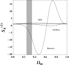
  Figure 4: This figure shows the evolution of the Statefinder $S_{4}^{(1)}$ plotted against $\Omega_{m}$.

• Galileon model [19, 20, 21, 22, 23]:

  The Galileon is a massless scalar field ($\pi$); whose action is invariant under the Galilean transformation  $\pi(x)\rightarrow\pi(x)+b_{\mu}x^{\mu}+c$, where $b_{\mu}$ and $c$ are the constant four vector and scalar respectively. Following Ref. [20], we consider the galileon action

  $$\mathcal{S}=\int{\textit{{\rm d}}^{4}x}\sqrt{-g}\left(\frac{R}{2}+c_{\textit{i}}~{}L^{(\textit{i})}\right)+\mathcal{S}_{m}[\psi_{m},e^{2\beta\pi}g_{\mu\nu}],$$ (3.8)

  where, ${c_{i}^{{}^{\prime}s}}$ are constants, $\beta$ is coupling of field with matter and $L_{i}^{{}^{\prime}s}$ [20] are Lagrangians for Galileon field. $L_{1}$ is linear in field and is often omitted assuming $c_{1}=0$, $L_{2}$ represents the standard kinetic term, $L_{3}=(\partial_{\mu}\pi)^{2}\Box\pi$ is the third order galileon term which occurs in DGP; $L_{4}$ and $L_{5}$ are higher order Lagrangians. Following Ref. [20], we shall consider Galileon Lagrangian upto $L_{4}$, sufficient to obtain a stable de Sitter solution. As for the parameters ${c_{i}^{{}^{\prime}s}}$ and $\beta$, we adopt the choice of the said reference which gives rise to a viable late time cosmology. It is interesting to note that the observational constraint on $\beta$($\beta\leq 0.1$) found in Ref. [20] was independently confirmed by the observed limit on the time variation of Newtonian constant $G$ [24]. Following this development, we shall use the numerical value of $\beta=0.1$ in the statefinder analysis.

  In this case, the evolution equations in a spatially flat background have the form [20]:

  $$3H^{2} = \rho_{m}+\frac{c_{2}}{2}\dot{\pi}^{2}-3c_{3}H\dot{\pi}^{3}+\frac{45}{2}c_{4}H^{2}\dot{\pi}^{4},$$ (3.9)

  $$2\dot{H}+3H^{2} = -\frac{c_{2}}{2}\dot{\pi}^{2}-c_{3}\dot{\pi}^{2}\ddot{\pi}+\frac{3}{2}c_{4}\dot{\pi}^{3}\left(3H^{2}\dot{\pi}+2\dot{H}\dot{\pi}+8H\ddot{\pi}\right),$$ (3.10)

  $$\beta\rho_{m} = -c_{2}\left(3H\dot{\pi}+\ddot{\pi}\right)+3c_{3}\dot{\pi}\left(3H^{2}\dot{\pi}+\dot{H}\dot{\pi}+2H\ddot{\pi}\right)$$ (3.11)

  $$-18c_{4}H\dot{\pi}^{2}\left(3H^{2}\dot{\pi}+2\dot{H}\dot{\pi}+3H\ddot{\pi}\right).$$

  The effective equation of state $w_{eff}$, equation of state $w_{\pi}$ and Hubble parameter for galileon model have the form

  $$w_{eff} = -\frac{2}{3}\frac{\dot{H}}{H^{2}}-1,$$ (3.12)

  $$w_{\pi} = \frac{p_{\pi}}{\rho_{\pi}},$$ (3.13)

  $$H^{2} = \frac{8\pi G}{3}\left[\rho_{0m}(1+z)^{3}+\rho_{\pi}\right],$$ (3.14)

  where,

  $$p_{\pi} = \frac{c_{2}}{2}\dot{\pi}^{2}+c_{3}\dot{\pi}^{2}\ddot{\pi}-\frac{3}{2}c_{4}\dot{\pi}^{3}\left(3H^{2}\dot{\pi}+2\dot{H}\dot{\pi}+8H\ddot{\pi}\right),$$

  $$\rho_{\pi} = \frac{c_{2}}{2}\dot{\pi}^{2}-3c_{3}H\dot{\pi}^{3}+\frac{45}{2}c_{4}H^{2}\dot{\pi}^{4}.$$

  $\begin{array}[]{c@{\hspace{0.4in}}c}\lx@intercol\mbox{}\hfil\lx@intercol&\lx@intercol\mbox{}\hfil\lx@intercol\\[0.0pt] \epsfbox{s32.eps}\hfil\hfil\hskip 28.90755pt&\epsfbox{s42.eps}\hfil\\[5.69046pt] \mbox{\bf(a)}\hfil\hskip 28.90755pt&\mbox{\bf(b)}\end{array}$

  Figure 5: The panels (a), (b) show the Statefinder $S_{3}^{(2)}$, $S_{4}^{(2)}$ plotted against $\Omega_{m}$. The dark energy models are: bimetric (dashed line), galileon (solid line), DGP (dotdashed line). The horizontal black line shows LCDM. The vertical band centered at $\Omega_{0{\rm m}}=0.3$ roughly corresponds to the present epoch.

  

  Figure 6: The Statefinders $S_{4}^{(1)}$ and $S_{3}^{(1)}$ are shown for different dark energy models; the arrows and dots show time evolution and present epoch respectively. LCDM corresponds to fixed point (1,1). We assumed, $\Omega_{0{\rm m}}=0.3$ (present epoch).

  Figure 7: This figure shows the evolution of $S_{4}$ and $S_{4}^{(1)}$ versus redshift z. For $\Lambda$CDM, $S_{4}^{(1)}:=S_{4}=1$, and for other dark energy models the two definitions $S_{4}$ and $S_{4}^{(1)}$ have different values. Top panels show $\Lambda$CDM (solid line), galileon (dotdashed line) and DGP models (dashed line) while bottom panels show the above models as well as the bimetric model (dotted line). From the top panel, one notes that $S_{4}^{(1)}$ provides a somewhat better diagnostic than $S_{4}$.

  Figure 8: Top, middle and bottom panels are for DGP, galileon and bimetric models respectively. In all panels, $\Omega_{0{\rm m}}$=0.25 (dotdashed line), $\Omega_{0{\rm m}}$=0.3 (dashed line), $\Omega_{0{\rm m}}$=0.35 (solid line) and $\Lambda$CDM (horizontal solid line). The effect of $\Omega_{0{\rm m}}$ on $S_{3}$ is more severe than $S_{2}$ as $S_{3}$ has cube power of $H$ in the denominator.

• The DGP model [25]:

  $$\frac{H(z)}{H_{0}}=\left[\left(\frac{1-\Omega_{0{\rm m}}}{2}\right)+\sqrt{\Omega_{0{\rm m}}(1+z)^{3}+\left(\frac{1-\Omega_{0{\rm m}}}{2}\right)^{2}}\right]\,\,$$ (3.15)

In order to apply the statefinder analysis to the models under consideration, we notice that the deceleration parameter q, statefinder pair $\{r,s\}$ and snap $\alpha_{4}$ can be easily expressed in terms of Hubble parameter $H(z)$ and its derivatives as follows:

$$q(z) = (1+z)\frac{H^{\prime}}{H}-1,$$

$$r(z) = 1-2(1+z)\frac{H^{\prime}}{H}+(1+z)^{2}\left(\frac{H^{\prime\prime}}{H}+\frac{H^{\prime 2}}{H^{2}}\right),$$

$$s(z) = \frac{r(z)-1}{3(q(z)-1/2)},$$

$$\alpha_{4}(z) = 1-3(1+z)\frac{H^{\prime}}{H}+(1+z)^{2}\left(\frac{H^{\prime\prime}}{H}+3\frac{H^{\prime 2}}{H^{2}}\right)$$ (3.16)

$$-(1+z)^{3}\left(\frac{H^{\prime\prime\prime}}{H}+4H^{\prime}\frac{H^{\prime\prime}}{H^{2}}+\frac{H^{\prime 3}}{H^{3}}\right),$$

where, $H$ is given by (3.6), (3.14) and (3.15) for different dark energy models discussed in the literature.

We are now in a position to present the numerical results for statefinder parameters for each model and strike a comparision between them. In figure 2, we show the time evolution of the statefinder pairs $\{r,s\}$ and $\{r,q\}$ for bimetric model of massive gravity and DGP model. One can see that both the models are differentiated by statefinder pairs. The statefinder hierarchy is used for higher derivatives of scale factor; which can easily distinguish different dark energy models. In figure 3, the behavior of bimetric, galileon and DGP models show nondegeneracy around the present value of $\Omega_{m}$ in $S_{2}-\Omega_{m}$ and $S_{3}-\Omega_{m}$ plane.

In figure 4, galileon model is highly degenerate, DGP model is nearly degenerate whereas bimetric model of massive gravity is showing nondegeneracy around the present value of $\Omega_{m}$. In $S_{3}^{(2)}-\Omega_{m}$ plane, galileon and bimetric models are nearly degenerate whereas DGP model is nondegenerate, around the present value of $\Omega_{m}$, as shown in figure 5 (a). In $S_{4}^{(2)}-\Omega_{m}$ plane, galileon model is highly degenerate, DGP model is nearly degenerate whereas bimetric model of massive gravity is nondegenerate, around the present value of $\Omega_{m}$, as shown in figure 5 (b). In figure 6, we exhibit the phase portrait in $S_{4}^{(1)}-S_{3}^{(1)}$ plane, where degeneracies among different dark energy models are broken.

Particularly, we should comment on $S_{2}-\Omega_{m}$, $S_{3}-\Omega_{m}$ and $S_{4}^{(1)}-S_{3}^{(1)}$ planes. From figures 3 and 6, one can clearly see that both the figures do not have degeneracies among $\Lambda$CDM, bimetric, galileon and DGP models around the present value of $\Omega_{m}$. At higher redshift (corresponding to $\Omega_{m}\simeq 0.7$), $S_{3}^{(2)}$ does an excellent job in distinguishing between the different DE models, as shown in figure 5 (a). Other statefinder hierarchy does not seem to perform well in distinguishing the different dark energy models considered in this paper. While carrying out comparison between $S_{2}$ and $S_{3}$, we note that Statefinder $S_{2}$ is easier to determine as it requires only two derivatives of the expansion factor whereas $S_{3}$ requires three. Since $S_{2}$, explicitly depends upon $\Omega_{m}$, it might look at the onset that it would exhibit more sensitivity to $\Omega_{0{\rm m}}$ than $S_{3}$. However, we should keep in mind that both $S_{2}$ and $S_{3}$ also implicit dependence on $\Omega_{0{\rm m}}$ through Hubble parameter; they contain $H^{2}$ and $H^{3}$ terms in the denominator respectively. Indeed, our numerical simulation shows that uncertainties in the value of $\Omega_{0{\rm m}}$ affect $S_{3}$ more severely than $S_{2}$, as demonstrated in figure 8, where $S_{2}$ and $S_{3}$ are plotted against redshift z. But when $S_{2}$ and $S_{3}$ are plotted against $\Omega_{m}$, there are no effects on $S_{2}$ and $S_{3}$ for different values of $\Omega_{0{\rm m}}$, as shown in figure 3 (though this figure is plotted for $\Omega_{0{\rm m}}=0.3$, it is checked that the results are same for other values). An important comment on the relative matter density dependence of $S_{2}$ and $S_{3}$ is in order. We know that $S_{3}$ depends solely on the third derivative of the scale factor $a(t)$ and its value can be determined from observations of the luminosity distance $D_{L}$ or the Hubble parameter, after differentiation. It is important to note that the value of the matter density does not enter into the expression of $S_{3}$. Therefore, if the observed value of $S_{3}$ departs from unity, it will give an important information about the nature of dark energy, namely, that dark energy is something beyond cosmological constant. On the other hand, a similar argument does not hold for $S_{2}$ since its value explicitly depends upon $\Omega_{m}$ and so the latter needs to be known (from observation) even after the differentiation of $D_{L}$ of $H(z)$.

It is interesting to note that Planck results favor larger values of $\Omega_{0{\rm m}}$ than SN$1$a and this is well reflected in the vertical band around $\Omega_{0{\rm m}}\simeq 0.3$ in most of the figures. The fact that an incorrect value of matter density could significantly bias the reconstructed value of $\omega(z)$ was discussed in [26].

4 Conclusion

In this paper we have shown that the bimetric model of massive gravity and the DGP model can be distinguished by using the statefinder pairs $\{r,s\}$ and $\{r,q\}$. We also carried out comparison between bimetric theory of massive gravity, galileon modified gravity and other popular dark energy models using the statefinder hierarchy in concordance cosmology. Our investigation in $S_{2}-\Omega_{m}$ and $S_{3}-\Omega_{m}$ planes show nondegeneracy among $\Lambda$CDM, bimetric, galileon and DGP models around the present value of $\Omega_{m}$, and all models considered in this paper are successfully differentiated by statefinder hierarchy on these planes. We have also noticed that our analysis presents a good comparison among the different dark energy models considered in this paper. Figures 3 and 6 show nondegeneracy among popular dark energy models around the present value of $\Omega_{m}$. We find that $S_{4}^{(1)}$, $S_{3}^{(2)}$ and $S_{4}^{(2)}$ do not perform well in distinguishing the different dark energy models considered in this paper, as shown in figures 4 and 5 . By looking at the success of the statefinder hierarchy diagnostic, we are encouraged to apply the analysis to models of extended massive gravity discussed in the literature.

We have demonstrated that $S_{2}$ and $S_{3}$ perform better than the higher order statefinders in discriminating between $\Lambda$CDM and modified gravity models of dark energy. While comparing between $S_{2}$ and $S_{3}$, we find that the statefinder $S_{2}$ is better discriminant than $S_{3}$, as demonstrated in figure 3. A comment about the possibility of observational constraints on the statefinder parameters is in order. Since these parameters include higher time derivatives, it is really challenging to measure them with good accuracy. One must wait until Euclid for a precise determination of this diagnostic, which is a very exciting possibility, since Euclid is most likely to take off and the data should be available within about a decade. Meanwhile as demonstrated in Ref. [7], one can use mean statefinder statistics using SNAP type experiment to distinguish various models. Other mean diagnostics are discussed in Refs. [5, 27]

References

- [1] S. Perlmutter et al., Measurements of Omega and Lambda from 42 High-Redshift Supernovae, Astrophys. J. 517, 565 (1999).
- [2] A. G. Riess et al. [Supernova Search Team Collaboration], Observational Evidence from Supernovae for an Accelerating Universe and a Cosmological Constant, Astron. J. 116 (1998) 1009;
- [3] E. Komatsu, et al., Seven-Year Wilkinson Microwave Anisotropy Probe (WMAP) Observations: Cosmological Interpretation, ApJS, 192, 18 (2011).
- [4] E. J. Copeland, M. Sami and S. Tsujikawa, Dynamics of dark energy, Int. J. Mod. Phys. D 15, 1753 (2006)[hep-th/0603057]; V. Sahni and A. A. Starobinsky, The Case for a Positive Cosmological Lambda-term, Int. J. Mod. Phys. D 9, 373 (2000); M. Sami, A primer on problems and prospects of dark energy, Curr. Sci. 97, 887 (2009) [arXiv:0904.3445].
- [5] V. Sahni, A. Shafieloo and A. A. Starobinsky, Two new diagnostics of dark energy, Phys. Rev. D 78, 103502 (2008).
- [6] A. Shafieloo, V. Sahni and A. A. Starobinsky, New null diagnostic customized for reconstructing the properties of dark energy from baryon acoustic oscillations data, Phys. Rev. D 86, 103527 (2012).
- [7] V. Sahni, T. D. Saini, A. A. Starobinsky and U. Alam, Statefinder – a new geometrical diagnostic of dark energy, JETP Lett. 77, 201 (2003); [arXiv:astro-ph/0201498].
- [8] U. Alam, V. Sahni, T. D. Saini and A. A. Starobinsky, Exploring the Expanding Universe and Dark Energy using the Statefinder Diagnostic , Mon. Not. Roy. Ast. Soc. 344, 1057 (2003).
- [9] M. Visser, Jerk, snap, and the cosmological equation of state , Class. Quant. Grav. 21, 2603 (2004).
- [10] M. Sami, M. Shahalam, M. Skugoreva, A. Toporensky, Cosmological dynamics of nonminimally coupled scalar field system and its late time cosmic relevance, Phys. Rev. D 86, 103532 (2012).
- [11] M. Arabsalmani, V. Sahni,The Statefinder hierarchy: An extended null diagnostic for concordance cosmology, Phys. Rev. D 83, 043501 (2011).
- [12] L.P. Chimento, A. S. Jakubi, D. Pavon and W. Zimdahl, Interacting quintessence solution to the coincidence problem, Phys.Rev. D 67, 083513 (2003) [astro-ph/0303145]; L. Zhang, J. Cui, J. Zhang, and X. Zhang, Interacting model of new agegraphic dark energy: Cosmological evolution and statefinder diagnostic, Int. J. Mod. Phys. D 19, 21 (2010) [arXiv:0911.2838]; A. Khodam-Mohammadi and M. Malekjani, Cosmic Behavior, Statefinder Diagnostic and Analysis for Interacting NADE model in Non-flat Universe, Astro- phys. Space Sci.331:265-273 (2011) [arXiv:1003.0543]; Z. L. Yi and T. J. Zhang, Statefinder diagnostic for the modified polytropic Cardassian universe, Phys.Rev.D75, 083515 (2007) [astro-ph/0703630]; M. Tong, Y. Zhang and T. Xia, Statefinder parameters for quantum effective Yang-Mills condensate dark energy model, Int. J.Mod. Phys.D18, 797 (2009) [arXiv:0809.2123]; H. Farajollahi and A. Salehi, Attractors, Statefinders and Observational Measurement for Chameleonic Brans–Dicke Cosmology, JCAP 1011:006 (2010) [arXiv:1010.3589].
- [13] U. Alam and V. Sahni, Confronting braneworld cosmology with supernova data and baryon oscillations, Phys. Rev. D 73, 084024 (2006), Z. K. Guo, Z. H. Zhu, J. S. Alcaniz, Y. Z. Zhang, Constraints on the DGP Model from Recent Supernova Observations and Baryon Acoustic Oscillations, Astrophys. J. 646 (2006) 1-7, [arXiv:astro-ph/0603632], R. Maartens and E. Majerotto, Observational constraints on self-accelerating cosmology, Phys. Rev. D 74, 023004 (2006).
- [14] V. Sahni, Y. Shtanov, Braneworld models of dark energy, JCAP 0311 (2003) 014, V. Sahni, Cosmological Surprises from Braneworld models of Dark Energy, [arXiv:astro-ph/0502032].
- [15] C. de Rham, G. Gabadadze and A..J. Tolley, Resummation of Massive Gravity, Phys. Rev. Lett. 106, 231101(2011).
- [16] S. Deser, A. Waldron, Acausality of Massive Gravity, Phys. Rev. Lett. 110, 111101 (2013), [arXiv: 1212.5835].
- [17] M. V. Strauss, A. Schmidt-May, J. Enander, E. Mortsell, and S. F. Hassan, Cosmological solutions in bimetric gravity and their observational tests, JCAP 03 (2012) 042, [arXiv:1111.1655].
- [18] Y. Akrami, T. S. Koivisto, M. Sandstad, Accelerated expansion from ghost-free bigravity: a statistical analysis with improved generality, JHEP, 03 (2013) 099, [arXiv:astro-ph/1209.0457].
- [19] C. Deffayet, S. Deser, and G. Esposito-Farese, Generalized Galileons: All scalar models whose curved background extensions maintain second-order field equations and stress tensors, Phys. Rev. D 80, 064015 (2009).
- [20] Amna Ali, R. Gannouji and M. Sami, Modified gravity a ‘la Galileon: Late time cosmic acceleration and observational constraints, Phys. Rev. D 82, 103015 (2010); R. Gannouji and M. Sami, Galileon gravity and its relevance to late time cosmic acceleration, Phys. Rev. D 82, 024011 (2010).
- [21] A. Nicolis, R. Rattazzi and E. Trincherini, The galileon as a local modification of gravity, Phys. Rev. D 79 (2009) 064036.
- [22] A. De Felice and S. Tsujikawa, Cosmology of a covariant Galileon field, Phys. Rev. Lett. 105, 111301 (2010).
- [23] S. A. Appleby and E. V. Linder, The Paths of Gravity in Galileon Cosmology, JCAP 1203:043 (2012).
- [24] E. Babichev, C. Deffayet, G.E. Farese, Constraints on Shift-Symmetric Scalar-Tensor Theories with a Vainshtein Mechanism from Bounds on the Time Variation of G, Phys. Rev. Lett. 107, 251102 (2011);
- [25] G. Dvali, G. Gabadadze and M. Porrati, 4D Gravity on a Brane in 5D Minkowski Space, Phys. Lett. B 485, 208 (2000).
- [26] U. Alam, V. Sahni, A. A. Starobinsky , Exploring the Properties of Dark Energy Using Type Ia Supernovae and Other Datasets, JCAP 0702 (2007) 011.
- [27] A. Shafieloo, U. Alam, V. Sahni, A. A. Starobinsky, Smoothing Supernova Data to Reconstruct the Expansion History of the Universe and its Age, Mon.Not.Roy.Astron.Soc. 366 (2006) 1081-1095.