THERMOCAPILLARY MOTION

Abstract

Mechanical motion (convection) appears in a nonuniformly heated liquid because its density depends on temperature¹⁾. This flow causes the liquid to self-mix unifying the temperature field. The convective flows are addressed in a series of papers recently published [1]. When the liquid has an interface, besides the convection, a different kind of a motion can appear. The origin of this motion is a gradient of the surface tension²⁾. Similarly to the electrocapillary motion, one can call this new motion a thermocapillary motion. In the present paper we consider two classes of thermocapillary motion: motion of a liquid in an open container and motion of a liquid drop suspended in another liquid.

.1 Motion of liquid in a flat open container when a temperature gradient is applied along the liquid interface

Considering the motion of liquid in a flat container let us assume that width and length of the container are sufficiently larger than its depth. This assumption reduces considerably the complexity of equations of liquid motion. The component momentum equations for steady motion of a viscous incompressible liquid written in the Cartesian coordinates are

$$v_{x}\frac{\partial v_{x}}{\partial x}+v_{y}\frac{\partial v_{x}}{\partial y}+v_{z}\frac{\partial v_{x}}{\partial z}=-\frac{1}{\rho}\frac{\partial p}{\partial x}+\nu\Delta v_{x}+F_{x},$$

$$v_{x}\frac{\partial v_{y}}{\partial x}+v_{y}\frac{\partial v_{y}}{\partial y}+v_{z}\frac{\partial v_{y}}{\partial z}=-\frac{1}{\rho}\frac{\partial p}{\partial y}+\nu\Delta v_{y}+F_{y}\,,$$ (1)

$$v_{x}\frac{\partial v_{z}}{\partial x}+v_{y}\frac{\partial v_{z}}{\partial y}+v_{z}\frac{\partial v_{z}}{\partial z}=-\frac{1}{\rho}\frac{\partial p}{\partial z}+\nu\Delta v_{z}+F_{z}\,.$$

Here F is an external body force³⁾.

Let us introduce an origin of coordinate system on the interface of liquid. The $x$- and $y$-axes are applied along the container length and width, respectively, the $z$-axis is directed from the liquid interface down to the bottom of the container. We assume a constant temperature gradient is applied along the $x$-axis, giving us $v_{y}=0$.

We will also neglect the convective flow because the depth of the container is smaller than its length. Feasibility of this assumption and the limitations which it causes for the theory will be addressed below. Now, since we disregarded the convective motion, then far away from the container walls $v_{z}=0$. Further, the term $\partial v_{x}/\partial x\sim v_{x}/l$ ($l$ is the container length) is much smaller than $\partial v_{x}/\partial z\sim v_{x}/h$ ($h$ is a depth of the container) and can be omitted, too. As a result of this simplifications, the system (1) is reduced to only two equations. The first one is

$$\frac{\partial p}{\partial x}=\mu\frac{\partial^{2}v_{x}}{\partial z^{2}}\,.\vspace*{0.2cm}$$ (2)

Liquid in the container is dragged by the moving surface layer, then it returns backward due to the container walls causing the appearance of a pressure drop along the $x$-axis. The second equation is

$$\frac{\partial p}{\partial x}=\rho g\,.$$ (3)

After integrating this equation the solution is

$$p=p_{1}(x)+\rho gz\,.$$ (4)

Now we will define the boundary conditions for Eq. (2). First, on a solid boundary the liquid velocity vanishes, it gives us a first condition

$$v_{x}(z=h)=0\,.$$ (5)

Second, on a free liquid interface the components of a viscous-stress tensor are continuous. Since $v_{y}=v_{z}=0$, then only the one tensor component $p_{xz}$ is essential for us while the others are either equal to zero or are not important at all. The continuity of $p_{xz}$ results to the second boundary condition

$$\frac{\partial\sigma}{\partial x}=-{\mu\frac{\partial v_{x}}{\partial z}}\,\,\,\,\,\textrm{at}\,\,\,{z=0}\,,$$ (6)

where $\sigma$ is the surface tension. Besides the boundary conditions, the solution of Eq. (2) should meet an additional condition representing the fact that the average velocity over the container cross section equals to zero:

$$\frac{1}{h}\int_{0}^{h}v_{x}dz=0\,.$$ (7)

With due account of relation (4), equation (2) is easily integrated. Indeed, substituting Eq. (4) in Eq. (2) we have

$$\frac{dp_{1}(x)}{dx}=\mu\frac{d^{2}v_{x}}{dz^{2}}\,.$$

Since $p_{1}(x)$ does not depend on the coordinate $z$, the solution of Eq. (2) is

$$v_{x}=A+Bz+\frac{1}{2\mu}\frac{dp_{1}(x)}{dx}z^{2}\,.$$

Applying the boundary conditions we have

$$B=-\frac{1}{\mu}\frac{d\sigma}{dx}\,,$$

$$A=\frac{h}{\mu}\frac{d\sigma}{dx}-\frac{1}{2\mu}\frac{dp_{1}(x)}{dx}h^{2}\,,$$

and finally the expression for the velocity is

$$v_{x}=\frac{1}{\mu}\frac{d\sigma}{dx}(h-z)-\frac{1}{2\mu}\frac{dp_{1}(x)}{dx}(h^{2}-z^{2})\,.$$

Applying this formula to condition (7) gives

$$\frac{dp_{1}(x)}{dx}=\frac{3}{2h}\frac{d\sigma}{dx}\,,$$

and for the pressure in the liquid we have

$$p=p_{0}+\frac{3}{2h}[\sigma(x)-\sigma(0)]+\rho gz\,,$$ (8)

where the constant $p_{0}$ cannot be found because the pressure in liquid is always defined to the extent of an additive constant. Finally, it gives us the velocity function in the liquid

$$v_{x}=\frac{1}{4\mu h}\frac{d\sigma}{dx}(3z^{2}-4hz+h^{2})\,,$$ (9)

or

$$v_{x}=\frac{1}{4\mu h}\frac{d\sigma}{dT}\frac{dT}{dx}(3z^{2}-4hz+h^{2})\,.$$ (10)

The profile of the velocity field is shown in Fig. 1.

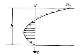
Figure 1: The profile of the velocity field for thermocapillary motion in a flat long container.

One can see from Eq. (10) that velocity of the liquid reaches its maximum on the liquid interface

$$v_{x,\,max}=\frac{h}{4\mu}\frac{d\sigma}{dT}\frac{dT}{dx}\,.$$ (11)

Since ${d\sigma}/{dT}<0$, therefore along the interface, the velocity direction is opposite to the temperature gradient.

If one compares the expression for the maximal velocity of the thermocapillary flow⁴⁾ against the expression for the characteristic velocity of the convective flow, introduced below, then one may think that the convective flow could be simply disregarded for the condition of large container depth $h$. However, it is not the case. In fact, formula (11) cannot be used for any size of the container. Indeed, in the momentum equations we have neglected the term $v_{x}({\partial v_{x}}/{\partial x})\sim{v_{x}^{2}}/{l}$ comparing to $\nu({\partial^{2}v_{x}}/{\partial z^{2}})\sim\nu{|v_{x}|}/{h^{2}}$. In other words, we assumed that ${v_{x}^{2}}/{l}\ll\nu{|v_{x}|}/{h^{2}}$ or, equally, $h^{2}\ll{\nu l}/{|v_{x}|}$. Substituting Eq. (11) into the last expression, we have a validity criterion for the developed theory:

$$h^{3}\ll\frac{4\nu^{2}\rho l}{\left|\frac{d\sigma}{dT}\frac{dT}{dx}\right|}\,.$$ (12)

When this inequality is not valid, our theory is not valid too. Thus, we cannot argue that if the depth, $h$, of the container is large enough, then velocity of the thermocapillary flow overcomes velocity of the convective flow. One would also think that with unlimited growth of both sizes $h$ and $l$, the thermocapillary velocity could exceed its convective value, however it is not the case as well. There are two restrictions regarding this way.

a) The temperature gradient is constant for any size of the container. In this case, the temperature difference $\Delta T$ over the container is $\Delta T=T-T_{0}=\nabla Tl\sim h^{3}$, and the convective velocity⁵⁾ grows much faster than the thermocapillary one because the former depends on temperature difference $\Delta T$ and not on temperature gradient.

b) The temperature difference is constant. The expression for the maximal thermocapillary velocity can be rewritten as

$$|v_{x,\,max}|=\frac{1}{\mu}{\left|\frac{d\sigma}{dT}\right|}\frac{|\Delta T|}{l}h\,.$$

Consider the estimate most favorable for the thermocapillary flow⁶⁾

$$h^{3}\sim\frac{\nu^{2}\rho l}{\frac{|\Delta T|}{l}\left|\frac{d\sigma}{dT}\right|}\,.$$

Then we have

$$|v_{x,\,max}|\sim\displaystyle{\frac{|\Delta T|^{{2/3}}\left|\frac{d\sigma}{dT}\right|^{2/3}}{\nu^{1/3}\rho^{2/3}l^{1/3}}}\,.$$

Thus, the maximal velocity increases with growth of the temperature difference and temperature coefficient of surface tension and decreases with the growth of viscosity and density. This is obvious. The most important result is the dependence of maximal velocity on the container size $l$. It is seen that under fixed temperature difference the maximal velocity of thermocapillary flow decreases with growth of $l$.

Assuming the following values for the parameters $\mu=0.01$ P, $dT/dx=0.1$ K/cm, $h=3$ cm, $d\sigma/dT=-0.15$ erg/(cm²K), involved in the thermocapillary velocity expression, we calculate the maximal velocity value $v_{x,\,max}=1.1$ cm/s ⁷⁾.

$\blacktriangledown$

Let us compare this estimate with the value of the convective velocity at the same conditions. The expression for the convective velocity has a form [1] ⁸⁾

$$\hskip 65.44142ptv_{\mathrm{conv}}=u_{z}\frac{x}{\delta}\left(1-\frac{x}{\delta}\right)^{2}\,,\hskip 65.44142pt(*)$$

where $\delta$ is the boundary layer thickness, $x\leq\delta$ and

$$u_{z}=5.17\nu\left(\frac{\nu}{\gamma}+\frac{20}{21}\right)^{-1/2}\left[\frac{g(T_{1}-T_{0})}{\nu^{2}T_{0}}\right]^{1/2}z^{1/2}\,,$$

$$\delta=3.93\left(\frac{\gamma}{\nu}\right)^{1/2}\left(\frac{\nu}{\gamma}+\frac{20}{21}\right)^{1/4}\left[\frac{g(T_{1}-T_{0})}{\nu^{2}T_{0}}\right]^{-1/4}z^{1/4}\,.$$

Here $g$ is the gravity, $T_{1}$ and $T_{0}$ are the temperatures of the wall and far from the wall, respectively, $\nu$ is the kinematic viscosity, $\gamma$ is the thermal diffusivity, $z$ is the nontrivial coordinate of a flat boundary layer. Since Ref. [1] does not provide an explicit expression for the convective velocity outside the boundary layer, we have to compare liquid fluxes rather than velocities:

$$J_{\mathrm{conv}}=\rho\int_{0}^{\delta}u_{\mathrm{conv}}dx=\frac{1}{6}u_{z}\delta\rho\,.$$

Substituting here $u_{z}$ and $\delta$ we find⁹⁾

$$J_{\mathrm{conv}}=3.4\mu\left(\frac{\gamma}{\nu}\right)^{1/2}\left(\frac{\nu}{\gamma}+\frac{20}{21}\right)^{-1/4}\left[\frac{g(T_{1}-T_{0})}{\nu^{2}T_{0}}\right]^{1/4}h^{3/4}\,.$$

The corresponding relation for the thermocapillary flux equals

$$J_{\mathrm{th-cap}}=\rho\int_{0}^{h/3}v_{x}dz=\frac{h^{2}}{27\nu}\frac{d\sigma}{dT}\frac{dT}{dx}\,.$$

Using the values of parameters mentioned above and $\rho=1$ g/cm³, $T_{1}-T_{0}=1$ K, $T_{0}=300$ K, we obtain the following estimates for both flows: $J_{\mathrm{conv}}=0.23$ g/(cm$\cdot$s) and $J_{\mathrm{th-cap}}=0.5$ g/(cm$\cdot$s). Thus, the thermocapillary mass flux proves to be prevailing over the convective one. Note, the given estimates are true for fairly large temperature gradients¹⁰⁾. If the temperature gradient was of the order of 0.01 K/cm ¹¹⁾, our conclusion would be changed to the opposite one and now the convective flow would dominate. Thus, one can conclude that the thermocapillary motion is negligible in all practically interesting situations. However, this is not true for some experiments where the heating of liquid is caused by applying the light on its surface. In this case a liquid is heated in a very thin layer near the free surface. For the considered termocapillary problem, this ‘skin layer’ doest not mean anything because the thermocapillary velocity depends on the total thickness of the liquid layer. For the convective flow, however, this ‘skin layer’ has a principal meaning because it is a variable in the velocity expression. For the lower values of the ‘skin layer’ $\sim\frac{1}{10}$ of the total thickness of the liquid layer, the thermocapillary flow dominates again. At lower values of the ‘skin layer’ just the convective flow becomes negligible.

$\blacktriangle$

.2 Motion of a drop in viscous medium due to temperature gradient

Let us consider now the problem of motion in a temperature field of a liquid drop suspended in another liquid. Because of the temperature difference at different points of the drop surface, the later cannot remain at rest. Instead, it will move from the warmer regions with the lower surface tension toward the colder regions with the higher surface tension. In the same moment the moving drop will drag the surrounding liquid medium by applying some force to it. There will also be an equal force in opposite direction which the surrounding medium will apply onto the drop. This reactive force will cause a drop movement in the direction of the temperature gradient.

Let us estimate the order of the thermocapillary velocity of the drop. The characteristic force applied per unit length of the nonuniformly heated surface is of the order of $\left|\frac{d\sigma}{dT}\nabla T\right|$. This force is balanced by the viscous forces¹²⁾:

$$\frac{\mu u}{a}+\frac{\mu^{\prime}u^{\prime}}{a}\sim\left|\frac{d\sigma}{dT}\nabla T\right|\,$$

Therefore we obtain

$$u\sim\frac{a\left|\frac{d\sigma}{dT}\nabla T\right|}{\mu+\mu^{\prime}}\,.$$

The exact value of the thermocapillary velocity can be found by solving the hydrodynamic equations with the appropriate boundary conditions. We will use the hydrodynamic equations within the Stokes approximation, because in all practical cases both the thermocapillary velocity and the Reynolds number are small

$$\nabla p=\mu\Delta\textbf{v}\,, \,\,\,\,\,\nabla p^{\prime}=\mu^{\prime}\Delta\textbf{v}^{\prime}\,,$$

$$\textrm{div}\,\textbf{v}=0\,, \,\,\,\,\,\ \textrm{div}\,\textbf{v}^{\prime}=0\,.$$ (13)

Here and below the variables with primes denote the liquid domain of the drop, while the variables without primes relate to the surrounding liquid. Let us consider the problem in the polar coordinate system attached to the moving drop and with the origin in the drop center. We chose the polar axes along the temperature gradient. The velocity is defined to be positive when it is directed along the polar axis. The boundary conditions far from the drop are

$$v_{\tau}|_{r\rightarrow\infty}\rightarrow u\cos\theta\,,\,\,\,v_{\theta}|_{r\rightarrow\infty}\rightarrow-u\sin\theta\,.$$ (14)

At the drop surface the following components of the stress tensor are continuous¹³⁾

$$(p^{0}_{rr}+p_{rr}^{\sigma})|_{r=a}=p_{rr}^{0}{}^{\prime}|_{r=a}\,,$$

$$(p^{0}_{r\theta}+p_{r\theta}^{\sigma})|_{r=a}=p_{r\theta}^{0}{}^{\prime}|_{r=a}\,.$$ (15)

In addition, at the drop surface the following conditions are true

$$v_{r}|_{r=a}=v^{\prime}_{r}|_{r=a}=0\,,\,\,\,\,\,\,v_{\theta}|_{r=a}=v^{\prime}_{\theta}|_{r=a}\,.$$ (16)

Here $v_{r}$, $v_{\theta}$, $v^{\prime}_{r}$, $v^{\prime}_{\theta}$ are the corresponding components of the velocity field. The stress tensor components are

$$p^{0}_{rr}=-p+2\mu\frac{\partial v_{r}}{\partial r}\,,$$

$$p^{\sigma}_{rr}=-\frac{2\sigma}{a}\,,$$

$$p^{0}_{r\theta}=\mu\left(\frac{\partial v_{\theta}}{\partial r}+\frac{1}{r}\frac{\partial v_{r}}{\partial\theta}-\frac{v_{\theta}}{r}\right)\,,$$ (17)

$$p^{\sigma}_{r\theta}=\frac{1}{a}\frac{\partial\sigma}{\partial\theta}\,.$$

Expressions for the variables with primes, $p_{rr}^{0}{}^{\prime}$, $p_{r\theta}^{0}{}^{\prime}$, are analogous to those for $p_{rr}^{0}$ and $p_{r\theta}^{0}$ with the obvious substitutions of unprimed functions by their primed counterparts. Because of the uniaxial symmetry of our problem, the velocity component $v_{\varphi}=0$ and all the variables of the problem are independent on the azimuthal angle $\varphi$. The surface tension is a part of boundary conditions and depends on the distribution of temperature on the drop interface.

We assume that the motion of the drop does not affect the distribution of temperature in the surrounding liquid, because the drop moves very slow. The temperature inside the drop is as if the drop had stayed at its particular location long enough. In addition, we assume the temperature gradient to be constant. Therefore the temperature distribution in both the drop and the surrounding liquid is described by the expression

$$T=T_{c}+|\nabla T|r\cos\theta\,,$$ (18)

where, $T_{c}$ is a temperature in the center of the drop. $T_{c}$ is a function of time

$$T_{c}=T_{0}+|\nabla T|ut\,.$$ (19)

Here $T_{0}$ is temperature in the center of the drop for initial drop position and $t$ is time. We also assume that the motion does not affect the drop spherical shape. Later, we will consider the feasibility of this assumption as well as its limits.

When the above assumptions are true, one can take the first spherical harmonic functions as a solution for the hydrodynamic equations [2].

The gradient of the surface tension caused by the inhomogeneous temperature on the interface is an origin of the motion on the drop surface. One can find the surface tension as a function of the angle $\theta$ using the following expression

$$\sigma=\sigma_{\pi/2}+\int_{\pi/2}^{\theta}\frac{d\sigma}{dT}\frac{\partial T}{\partial\theta}d\theta\,.$$

As a first approximation, one can assume that the derivative ${d\sigma}/{dT}$ does not depend on temperature and therefore on angle $\theta$. In this case, taking into account Eq. (18) one finds the surface tension

$$\sigma=\sigma_{\pi/2}+\frac{d\sigma}{dT}|\nabla T|a\cos\theta\,.$$ (20)

Now we insert the last expression to the boundary conditions (16) getting seven equations to obtain the eight constants $a_{0}$, $b_{0}$, $a_{1}$, $b_{1}$, $a_{2}$, $b_{2}$, $b_{3}$, $u$ ¹⁴⁾. As usual, one constant cannot be defined, so let us set $a_{0}=p_{0}$, where $p_{0}$ is a pressure in the center of the drop. The other constants are:

$$b_{0}=p_{0}-\frac{2\sigma_{\pi/2}}{a}\,,\hskip 21.33955ptb_{1}=0\,,$$

$$a_{1}=\frac{3}{2}\frac{u}{a^{2}}\,,\,\hskip 48.36958ptb_{2}=-a^{3}u\,,$$ (21)

$$a_{2}=-\frac{3}{2}u\,,\hskip 48.36958ptb_{3}=u=\frac{2}{3}\frac{\frac{d\sigma}{dT}|\nabla T|a}{2\mu+3\mu^{\prime}}\,.$$

The motion of liquid outside and inside the drop are described, correspondingly, by the following equations:

$$v_{r}=u\left(1-\frac{a^{3}}{r^{3}}\right)\cos\theta\,,\hskip 22.76228ptv^{\prime}_{r}=\frac{3}{2}u\left(\frac{r^{2}}{a^{2}}-1\right)\cos\theta\,,$$

$$v_{\theta}=-u\left(1+\frac{a^{3}}{2r^{3}}\right)\sin\theta\,,\hskip 8.5359pt\,v^{\prime}_{\theta}=\frac{3}{2}u\left(1-2\frac{r^{2}}{a^{2}}\right)\sin\theta\,,$$

$$p=p_{0}-\frac{2\sigma_{\pi/2}}{a}\,,\hskip 51.21504ptp^{\prime}=p_{0}+15\frac{\mu^{\prime}}{a^{2}}ur\cos\theta\,.$$

Velocity $u$ (this is velocity of the liquid at infinity) is opposite to the temperature gradient because of the relation ${d\sigma}/{dT}<0$ . Velocity of the drop is $-u$, it is aligned along the temperature gradient. Thus, the drop moves from the cooler layers of liquid to the warmer ones. It is apparent that this motion promotes the temperature leveling-off.

Let us compare the thermocapillary velocity of the drop with a maximal velocity of the thermocapillary flow in the container

$$\left|\frac{u_{\mathrm{drop}}}{u_{\mathrm{container}}}\right|=\frac{8\mu a}{3(2\mu+3\mu^{\prime})h}<\frac{4}{3}\frac{a}{h}\,.$$

Now, if one uses the characteristic values for the parameters $\mu=0.01$ P, $\mu^{\prime}=0.5$ P, $a=0.3$ mm, $|\nabla T|=0.1$ K/cm, $d\sigma/dT=-0.015$ erg/(cm${}^{2}\cdot$K) in the drop velocity expression, then one can estimate the drop velocity $u=2\cdot 10^{-4}$ cm/s¹⁵⁾.

We have mentioned above that assumption of the constant spherical shape of the drop should constrain our theory. Let us consider this constraint now. We believe that the drop keeps its shape nearly spherical when the surface tension on the drop interface is nearly constant, i.e., $|\sigma-\sigma_{\pi/2}|\ll\sigma_{\pi/2}$, where $\sigma_{\pi/2}$ is the surface tension on the drop’s equator and $\sigma$ is the surface tension in the any other point of the drop interface. Assuming this we can write

$$({d\sigma}/{dT})|\nabla T|a/{\sigma_{\pi/2}}\ll 1\,.$$ (22)

To make clear in which parameter regions our theory is applicable, let us consider a numerical example. The equator’s surface tension depends on the equator’s temperature, however, it is not significant regarding our estimate of the theory’s validity. Therefore for the values of the parameters given above we have $|\nabla T|a\ll 50\,\mathrm{K}\,.$ This inequality requires the temperature change along the drop perimeter to be less than $50$ K. It is clear that this inequality is almost always true. Indeed, for $|\nabla T|=0.1$ K/cm we should require the following inequality $a\ll 5$ m to be true. It is obvious that all drops in real experiments satisfy this condition.

One can show that the thermocapillary drop velocity can overcome (and sometimes, for some cases does so significantly) the electrocapillary drop velocity for weakly conductive drops.

I would like to thank V.G. Levich for giving this problem to my consideration and for his constant advice during my work.

.3 CONCLUSIONS

1. Two cases of the flow of liquid caused by the temperature gradient in the interfacial layer (thermocapillary flow) are considered. 2. Thermocapillary flow can overcome convective flow when the interfacial heating layer is reasonably small. 3. The limits of the theory’s applicability are discussed.

I Biographical sketch

Alexander I. Fedosov (13.09.1923–05.10.1999) was born in a small village in the northern region of the Saratov province of the former Soviet Union. After graduating from school with a gold medal, he became a student of the Moscow Pedagogical Institute. He graduated in 1945, and continued to the postgraduate program under the supervision of V.G. Levich. In 1948, A.I. Fedosov successfully defended his PhD thesis entitled ‘Some problems of the theory of surface phenomena’ in the Moscow Pedagogical Institute. He was unable of permanently stay in Moscow after getting his PhD, and he moved to Chita (Trans-Baikal region, Siberia) - a city 6,500 km away from Moscow. In the following period, from 1949 to 1955, A.I. Fedosov worked in the Chita Pedagogical Institute as a senior lecturer of physics. In 1955, A.I Fedosov moved to Kuibyshev (nowadays known as Samara), where he worked as an associate professor and a Head of the Department of Physics first in the Pedagogical Institute, then in the Agricultural Institute and at the end of his career in the Aviation Institute.

I.1 List of main publications of Fedosov¹⁶⁾

(a) A.I. Fedosov, Ph.D. thesis. Some problems of the theory of surface phenomena. Moscow State Pedagogical Institute. 1948. (In Russian).

(b) A.I. Fedosov, Electrocapillary motion of drops, Zhurnal Fizicheskoi Khimii 29, N5, p. 822-831 (1955). (In Russian).

(c) A.I. Fedosov, Effect of surfactant on the motion of drops in liquids, Zhurnal Fizicheskoi Khimii 30, N1, p. 223-227 (1956). (In Russian).

(d) A.I. Fedosov, Thermocapillary motion, Zhurnal Fizicheskoi Khimii 30, N2, p. 366-373 (1956). (In Russian).

(e) A.I. Fedosov, Drag of bubble movement by surfactant at moderate Reynolds numbers, Zhurnal Fizicheskoi Khimii 33, N8, p. 1681-1686 (1959). (In Russian).

References

- (1)
- (2) The current state of hydroaerodynamics of viscous fluid, V. 2. Ed.: S. Goldshtein, Moscow, 1948. (In Russian).
- (3) H. Lamb, Hydrodynamics (Dover, New York, 1945). References and footnoted supplements added by KM and VB
- (4) A.I. Fedosov, Ph.D. thesis. Some problems of the theory of surface phenomena. Moscow State Pedagogical Institute. 1948. (In Russian).
- (5) V.G. Levich, Physicochemical hydrodynamics. Englewood Cliffs, N.J., Prentice-Hall. 1962.
- (6) R.V. Birikh, Thermocapillary convection in a horizontal layer of liquid, Journal of Applied Mechanics and Technical Physics 7, N 3, pp. 43-44 (1966); DOI: 10.1007/BF00914697.