On computation of the total set of robust discrete-time PID controllers

Abstract

The problem of finding the set of all multi-model robust PID and three-term stabilizers for discrete-time systems is solved in this paper. The method uses the fact that decoupling of parameter space at singular frequencies is invariant under a linear transformation. The resulting stable regions are composed by convex polygonal slices. The design problem includes the assertion of intervals with stable polygons and the detection of stable polygons. This paper completes the solutions to both problems.

I INTRODUCTION

It has been shown that the stabilizing region for time-continuous PID-controllers is defined by a set of convex polygonal slices normal to $k_{P}$ axis in the $(k_{P},~{}k_{I},~{}k_{D})$ parameter space. Different approaches which prove this result use generalization of the Hermite-Biehler theorem, see [2], calculation of the real-axis intersections of the Nyquist plot, see [3] and singular frequencies, see [6], [1] and [5]. In the cited articles, it has been shown that the design of PID parameters due to decoupling of PID controller parameters at singular frequencies may be divided into two subproblems: (A) assertion of stable intervals of parameter $k_{P}$ independently on parameters $k_{I}$ and $k_{D}$ and (B) detection of stable polygons on the plane ($k_{I},~{}k_{D}$) for a given $k_{P}$. the solutions to problems (A) and (B) for the continuous-time systems can be found in [1] and [7].

In the present paper the time-continuous theory is transferred to the design of PID and three-term controllers in discrete-time domain. First related results are reported in [5], where the set of all Schur-stable controllers is shown to be composed by transformed polygonal slices in a parameter space ($r_{1},r_{2},r_{3}$). While a solution to the problem (B) as proposed in [7] applies directly in the discrete-time domain, see Section IV, this paper addresses the problem (A) in Section V. Section III proves that parameter decoupling applies in general at singular frequencies. Basically, a function is constructed from the characteristic polynomial, such that its imaginary part on each point on unity circle depends only on the gridding parameter (here conventionally chosen) $r_{3}$ and is independent on parameters $r_{1}$ and $r_{2}$. This result will lead to the conclusion that for a given plant a fixed number of singular frequencies must be available for its stabilization. Given that parameter $r_{3}$ defines uniquely the number of singular frequencies, one can directly discriminate the intervals of parameter $r_{3}$, which for no triple $(r_{1},~{}r_{2},~{}r_{3})$ can provide stabilization. The simplicity of the criterion is, however, achieved at the price of conservativeness, since just necessity is provided. To cope with conservativeness the approach proposed in [1] for the continuous-time case may be directly used. All aspects of the method are illustrated by examples.

II Problem definition

Consider a simple closed curve $\Gamma~{}=\{z\mid z=\tau(\alpha)+j~{}\eta(\alpha),~{}\alpha\in[a,~{}b]\}$, in $z-$plane, which is symmetric to the real axis $\tau$ and can be expressed in the form

$$\Gamma:~{}~{}F(\tau,\eta)=0,$$ (1)

and a characteristic equation of the form

$$p=A(z)Q(z,r_{1},r_{2},r_{3})+B(z)=0,$$ (2)

where $A$, $B$ are polynomials in $z$ and $r_{1},~{}r_{2},~{}r_{3}$ are real parameters, that enter linearly in $Q$,

$$Q=\delta_{1}(z)r_{1}+\delta_{2}(z)r_{2}+\delta_{3}(z)r_{3},$$ (3)

where the polynomials $\delta_{i}(z)$ are assumed to be of the order $\leq 2$ in $z$.

The following problem is handled in this article: Compute the set of all parameters $r_{1},r_{2},r_{3}$, such that the polynomial (2) is $\Gamma-$stable, that is, all its eigenvalues are enclosed by $\Gamma$. Of main interest in this article are circles with center on the real axis $\tau$ and an arbitrary radius, which will be referred to as $\Gamma-$circles. Especially important is the unity circle because of Schur-stability. $\Gamma-$region refers to the region enclosed by $\Gamma$.

It may be easily shown that (2) describes the characteristic equation of a feedback loop with a PID or a three-term controller. Indeed a discrete-time equivalent of the PID controller has the transfer function

$$C_{1}(z)=\frac{c_{1}+c_{2}z+c_{3}z^{2}}{(z+z_{1})(z-1)}.$$ (4)

Its structure follows in the quasi-continuous consideration by applying the rectangular integration rule $(s\rightarrow(z-1)/Tz)$ to the ideal PID controller $k_{I}/s+k_{P}+k_{D}s$, resulting in $z_{1}=0$, or by the trapezoidal integration rule $(s\rightarrow 2(z-1)/T(z+1))$, resulting in $z_{1}=1$. Also the realizable PID controller $k_{I}/s+k_{P}+k_{D}s/(1+T_{1}s)$ converts by the trapezoidal integration rule to the controller structure (4) with a pole at $z_{1}=-(2T_{1}-T)/(2T_{1}+T)$. The following derivation also holds for a three-term controller with an arbitrary second order denominator polynomial

$$C_{2}(z)=\frac{n(z)(c_{1}+c_{2}z+c_{3}z^{2})}{d(z)}.$$ (5)

For both controller structures, (4) and (5), the polynomial $Q$ is of the form

$$Q=c_{1}+c_{2}z+c_{3}z^{2}.$$ (6)

It is clear that (3) and (6) are connected via a parameter space transformation

$$c=T~{}r,~{}~{}\textrm{det~{}}T~{}\neq 0,$$ (7)

with $c=[c_{1},c_{2},c_{3}]^{T},~{}~{}r=[r_{1},r_{2},r_{3}]^{T}$. The rotation matrix $T$ is determined by the polynomials, $\delta_{1}(z),\delta_{2}(z),\delta_{3}(z)$.

III Basic definitions and theorems

Let $H$ and $G$ represent the real and imaginary part of the characteristic polynomial $p(z,r_{1},r_{2},r_{3})$ in (2) on $\Gamma$.

Definition 1

$\Gamma$ is said to be singular with respect to parameters $r_{1}$ and $r_{2}$ in (2) if

$$\textrm{Rank}\frac{\partial{}(H,G)}{\partial{}(r_{1},r_{2})}=1\qquad\textrm{for all }z\in{}\Gamma{}.$$ (8)

The latter equation is referred to as the rank-condition. Unless otherwise stated, $\Gamma$ will be assumed singular for the rest of the article. A zero of the polynomial (2), which additionally fulfills the rank-condition is referred to as singular frequency. For a fixed parameter $r_{3}$, singular frequencies are mapped to straight lines on the plane ($r_{1},r_{2}$) and the eigenvalues of (2) can cross over a singular $\Gamma$ just at singular frequencies.

Definition 2

A function $E_{\Gamma}(z)$ defined as

$$Q(z,r_{1},r_{2},r_{3})=E_{\Gamma}(z)~{}q(z,r_{1},r_{2},r_{3})$$ (9)

with

$$I_{q}=r_{3}g_{3}(\alpha)+g_{0}(\alpha),~{}~{}~{}\alpha\in[a,~{}b]$$ (10)

i.e. $\frac{\partial I_{q}}{\partial r_{1}}=\frac{\partial I_{q}}{\partial r_{2}}=0$, where $I_{q}$ stands for the imaginary part of $q$, will be referred to as decoupling function of $Q$ over $\Gamma$.

Lemma 1

If $\Gamma$ is singular then

$$\frac{\partial I_{q}}{\partial r_{1}}=0\Leftrightarrow\frac{\partial I_{q}}{\partial r_{2}}=0,~{}~{}~{}\forall z\in\Gamma.$$ (11)

Proof.  Consider the rank-condition (8). It may be checked that

$$\frac{\partial{}(H,G)}{\partial{}(r_{1},r_{2})}=\left(R^{2}_{A}+I^{2}_{A}\right)\left(R^{2}_{\phi}+I^{2}_{\phi}\right)\left(\frac{\partial R_{q}}{\partial r_{1}}\frac{\partial I_{q}}{\partial r_{2}}-\frac{\partial I_{q}}{\partial r_{1}}\frac{\partial R_{q}}{\partial r_{2}}\right)$$

If rank-condition applies, that is, the right-hand side of the above equation is zero, then $\frac{\partial I_{q}}{\partial r_{1}}=0\Rightarrow\frac{\partial I_{q}}{\partial r_{2}}=0$, since $\frac{\partial R_{q}}{\partial r_{1}}\neq 0$. Similarly, $\frac{\partial I_{q}}{\partial r_{2}}=0\Rightarrow\frac{\partial I_{q}}{\partial r_{1}}=0$. ∎

Theorem 1

Two decoupling functions of $Q$ in (3) over $\Gamma$ are simply given by

$$E_{\Gamma}(z)=\delta_{1}(z),~{}~{}~{}E_{\Gamma}(z)=\delta_{2}(z).$$ (12)

Proof. Suppose $E_{\Gamma}(z)=\delta_{1}(z)$. Then

$$q=r_{1}+\frac{\delta_{2}(z)}{\delta_{1}(z)}r_{2}+\frac{\delta_{3}(z)}{\delta_{1}(z)}r_{3},$$

and $\frac{\partial I_{q}}{\partial r_{1}}\equiv 0$. Lema 1 guarantees that for all $z\in\Gamma$ the imaginary part of $\frac{\delta_{2}(z)}{\delta_{1}(z)}$ is also zero, that is, (10) applies. Since $\frac{\delta_{2}(z)}{\delta_{1}(z)}$ is real on $\Gamma$, its inverse will be also real, that is, the imaginary part of $\frac{\delta_{1}(z)}{\delta_{2}(z)}$ for all $z\in\Gamma$ is zero. Hence, $\delta_{2}(z)$ represents also a decoupling function. ∎

The next statement may be directly checked.

Theorem 2

Consider the function

$$F(z):=\frac{p(z)}{A(z)E_{\Gamma}(z)}.$$ (13)

The equation $F(z)=0$ for $z\in\Gamma$ decouples the parameters $r_{1},r_{2}$ and $r_{3}$ into two equations

$$r_{1}h_{1}(\alpha)+r_{2}h_{2}(\alpha)+h_{0}(\alpha) = 0,$$ (14)

$$r_{3}g_{1}(\alpha)+g_{0}(\alpha) = 0.$$ (15)

The latter theorem is essential for solving the problem (A) as defined in the introduction of the article. The first equation refers to the generator of singular lines, and the second one to the generator of singular frequencies.

Finally, let $\{p_{\nu}\}$ represent a finite set of polynomials of the form (2), i.e.

$$p_{\nu}=A_{\nu}(z)Q(z,r_{1},r_{2},r_{3})+B_{\nu}(z).$$ (16)

For example, this may be a multi-model of a continuum of plants or Kharitonov polynomials of an interval uncertainty.

Theorem 3

The rank-condition (8) for the set of polynomials (16) does not depend on the polynomials $A_{\nu}(z)$ and $B_{\nu}(z)$.

Hence a singular $\Gamma$ is completely determined by the polynomial $Q$ in (3). Though the singularity of $\Gamma$ is not destroyed by polynomials $A_{\nu}(z)$ and $B_{\nu}(z)$, they influence the root-condition, i.e. the singular frequencies on $\Gamma$.

III-A Schur-stability

Consider the Schur-circle defined as $\Gamma_{1}~{}=\{e^{j\alpha}:~{}\alpha\in[-\pi,~{}\pi]\}$. It can be easily checked that the rank-condition (8) is satisfied over $\Gamma_{1}$ for

$$Q=(1+z^{2})r_{1}+zr_{2}+r_{3}$$ (17)

and that the matrix $T$, as defined in (7) is

$${T}=\left[\begin{array}[]{ccc}1&0&1\\ 0&1&0\\ 1&0&0\end{array}\right].$$ (21)

According to Theorem 1 the decoupling functions of (17) over the Schur-circle $\Gamma_{1}$ are

$$E_{\Gamma}(z)=1+z^{2}~{}~{}\textrm{or}~{}~{}E_{\Gamma}(z)=z.$$ (22)

Let $E_{\Gamma}(z)=z$. It may be easily shown that the imaginary part of the function

$$F(z)=\frac{1+z^{2}}{z}r_{1}+r_{2}+\frac{B(z)}{zA(z)}r_{3}$$ (23)

on the Schur-circle is of the form (10), that is imaginary part of $\frac{1+z^{2}}{z}$ is zero on the Schur-circle.

III-B $\Gamma$-stability

Consider a $\Gamma-$circle with center on real axis $\Gamma~{}=\{m+re^{j\alpha}$, $\alpha\in[-\pi,~{}\pi]\}$, Fig 1. Now it can be shown that

$$Q=(r^{2}-m^{2}+z^{2})r_{1}+(z-m)r_{2}+r_{3}.$$ (24)

For $\Gamma-$circles with center at $\tau=m$ and radius $r$ a transformation matrix from $c-$ to $r-$parameter space is checked to be,

$${T}=\left[\begin{array}[]{ccc}r^{2}-m^{2}&-m&1\\ 0&1&0\\ 1&0&0\end{array}\right]$$ (28)

A corresponding decoupling function is

$$E_{\Gamma}(z)=z-m$$ (29)

and

$$F(z)=\frac{r^{2}-m^{2}+z^{2}}{z-m}r_{1}+r_{2}+\frac{B(z)}{(z-m)A(z)}r_{3}.$$ (30)

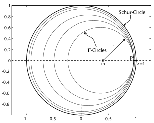
Figure 1: Schur- and $\Gamma-$circles

III-C Example

Consider the discrete-time model of the plant

$$G=10^{-6}\frac{4.165z^{3}+45.77z^{2}+45.77z+4.165}{z^{4}-3.985z^{3}+5.97z^{2}-3.985z+1},$$ (31)

and a three-term stabilizer

$$C(z)=10^{4}\frac{(z^{2}-1.541z+0.5992)(c_{1}+c_{2}z+c_{3}z^{2})}{z(z+0.4047)(z+0.2162)(z-0.4934)},$$ (32)

whose parameters $c_{1},c_{2},c_{3}$ should be synthesized. The synthesis is done in $(r_{1},r_{2},r_{3})$-parameter space. Therefore the transformation (21) can be used. Then

$$A = {z}^{5}+9.44z^{4}-5.34z^{3}-9.34z^{2}+5.04z+0.59$$ (33)

$$B = 0.19z^{8}-0.73z^{7}+z^{6}-0.45z^{5}-0.12z^{4}+\cdots$$ (34)

$$0.14z^{3}-0.009z^{2}-0.008z.$$

The equation (15) reads

$$r_{3}=\frac{C^{5}_{\alpha}-2.71\,C^{4}_{\alpha}+1.61\,C^{3}_{\alpha}+1.35\,C^{2}_{\alpha}-1.70\,C_{\alpha}+0.44}{0.02\,C^{4}_{\alpha}+0.08\,C^{3}_{\alpha}-0.13\,C^{2}_{\alpha}-0.08\,C_{\alpha}+0.11}.$$ (35)

where $C_{\alpha}=\cos(\alpha)$. For illustration purposes its plot is shown in Fig. 2. E.g. for $r_{3}=-0.26118$, the singular frequencies lying on the Schur-circle are computed to be

$$\begin{array}[]{lcl}\alpha^{\prime}_{1}=0&~{}~{}~{}\Rightarrow{}{}{}&z^{\prime}_{1}=1,\\ \alpha^{\prime}_{2}=\pm 0.4097&~{}~{}~{}\Rightarrow{}{}{}&z^{\prime}_{2}=0.9172\pm j0.3983,\\ \alpha^{\prime}_{3}=\pm 0.97300&~{}~{}~{}\Rightarrow{}{}{}&z^{\prime}_{3}=0.5628\pm j0.8266,\\ \alpha^{\prime}_{4}=\pm\pi&~{}~{}~{}\Rightarrow{}{}{}&z^{\prime}_{4}=-1.\end{array}$$ (40)

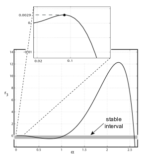
Figure 2: The generator fo singular frequencies; Equation 35

IV Stable convex polygons

Notice that the characteristic equation in (2) over singular $\Gamma$ decouples equivalently to the two equations in (14) and (15). For a fixed $r_{3}$ the equation (14) defines a set of singular frequencies $\{\alpha^{\prime}_{\nu}\}$ on $\Gamma$. The equation (15) determines the set of straight lines $\{\lambda_{\nu}\}$, which are determined by $\{\alpha^{\prime}_{\nu}\}$. Geometrically, the straight lines $\{\lambda_{\nu}\}$ represent the eigenvalue boundaries in the $(r_{1},r_{2})$-plane for the fixed parameter $r_{3}$. Thus, stable regions are composed by convex polygons and the design problem defined in the previous section is decoupled into two subproblems: (A) assertion of stable intervals of parameter $r_{3}$ independently on parameters $r_{1}$ and $r_{2}$ and (B) detection of stable polygons on the plane ($r_{1},~{}r_{2}$) for a given $r_{3}$.

For the sake of completion, this section recalls briefly the solution of problem (B), while problem (A) will be thoroughly discussed in the next section. For details the reader is referred to [7], [1]. The algorithm is motivated by the concept of inner polygons, which claim a necessary condition for stability: A polygon $\Pi$ is said to be an inner polygon if any transition over $\lambda_{\nu}$ inside the polygon causes an eigenvalue-pair to enter the $\Gamma-$region at the corresponding frequency.

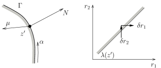
Figure 3: Definition of $e_{1}$ and $e_{2}$: the motion of eigenvalues in the vicinity of a singular frequency $z^{\prime}$. By convention, the shaded part refers to the stable side of $\Gamma$ and the normal $N$ points outside the $\Gamma$-region.

In order to automate the detection of an inner polygon each singular line $\lambda{}(\alpha^{\prime})$, will be assigned a ”transition” function $e$: it is negative if the transition $[\delta{}r_{1},\delta{}r_{2}]$ (see Fig. 3) over the singular line causes an eigenvalue to become stable, otherwise it is positive. Let $e_{1}$ correspond to $\delta{}r_{1}>0,~{}\delta{}r_{2}=0$ and $e_{2}$ to $\delta{}r_{2}>0,~{}\delta{}r_{1}=0$. In [7] it shown that the motion of eigenvalues at $z^{\prime}=\tau(\alpha^{\prime})\pm j\eta(\alpha^{\prime})$ defined as the scalar product $e=\mu N$ (see Fig. 3) is described by the equation

$$e_{1/2}:=\left(\frac{\partial F}{\partial\tau}\Bigg{|}\frac{\partial(H,G)}{\partial(\eta,r_{1/2})}\Bigg{|}+\frac{\partial F}{\partial\eta}\Bigg{|}\frac{\partial(H,G)}{\partial(r_{1/2},\tau)}\Bigg{|}\right)_{\normalsize\alpha^{\prime}}.$$ (41)

Using this information, an algorithm for the detection of the inner polygons with maximal $\Gamma$-stable eigenvalues may be developed, see [7]. Such polygons are the only candidates, which need to be checked for stability. To this end, it suffices to check any point within such a polygon.

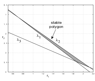
Figure 4: The stable polygon lying on the plane $r_{3}=-0.26118$

IV-A Example: (cont.)

Reconsider the plane $r_{3}=-0.26118$. The corresponding singular frequencies were computed in the previous section, (40). Each of these singular frequencies $z^{\prime}_{\nu}$ generates a straight line $\lambda_{\nu}$ on the plane $r_{3}=-0.26118$. The resulting stable polygon is shown in Fig. 4. It is enclosed by the straight lines frequencies $\lambda_{1},\lambda_{2}$ and $\lambda_{3}$, corresponding to $z^{\prime}_{1},z^{\prime}_{2}~{}\textrm{and}~{}z^{\prime}_{3}$.

V Stable gridding intervals

This section focuses on the problem how to discriminate $r_{3}-$intervals, such that stable polygons may exist therein. The basic idea presented here tempts to extrapolate this information from the plot of equation (15), see Fig. 2. Basically, one would like to link somehow the stability of the characteristic polynomial (2) with the number of singular frequencies on $\Gamma$. This approach is motivated by the fact that an emerging pair of singular frequencies produces new polygons and vice-versa.

The following lemma is essential for the main result of this section. Without loss of generality, the $\Gamma$-region is assumed to be a Schur-circle. The generalizations for $\Gamma-$circles are straightforward. Its proof is, however, beyond teh scope of this article (proof hints: (a) $N$ is always even, (b) the Mikhailov curve is symmetric to the real axis $\tau$ and (c) the poles on $\Gamma$ are avoided by infinitely small circles, whereby the Mikhailov plot experiences a phase shift of $\pm\pi$ at infinity.)

Lemma 2

Consider the Mikhailov plot of a function $F(e^{j\alpha})$ on the Schur-circle $\Gamma_{1}$ and let $F(z)$ possess $J$ poles $\neq\pm 1$ on $\Gamma_{1}$, a pole of the order $J_{+}$ at $z=+1$, and a pole of the order $J_{-}$ at $z=-1$. If the phase change of the Mikhailov vector $F(e^{j\alpha})$ over $\Gamma-1$ is $N\pi$ as $\alpha$ changes from $0$ to $+\pi$ without touching them, then it cuts the real axis at least $Z-$times, where

$$Z=\frac{N-J-2-E(J_{+})-E(J_{)}}{2}.\\$$ (42)

Theorem 4

Consider the characteristic polynomial (2) and the Schur-circle $\Gamma_{1}$. Let
$N$: order of the polynomial (2) $R$: number of zeros of $A(z)E_{\Gamma}(z)$ lying inside $\Gamma$ $J$: number of zeros $\neq\pm 1$ of $A(z)E_{\Gamma}(z)$ lying on $\Gamma$ $J_{+}$: order of the zero $+1$ of $A(z)E_{\Gamma}(z)$ $J_{-}$: order of the zero $-1$ of $A(z)E_{\Gamma}(z)$ $Z$: number of singular frequencies in the interval $0<\alpha<+\pi$.

A necessary condition for stability of (2) is

$$Z\geq N-R-\frac{J+E(J_{+})+E(J_{)}+2}{2}.$$ (43)

Proof.  As shown in Section III, the equation

$$F(z)=\frac{p(z)}{A(z)E_{\Gamma}(z)}=0$$ (44)

decouples parameters $r_{1},r_{2}$ and $r_{3}$ into the two equations (14) and (15), whereby the imaginary part represents the generator of singular frequencies. The Mikhailov plot of function $F(z),~{}z=\tau(\alpha)+j\eta(\alpha)),~{}-\pi\leq\alpha\leq\pi$ intersects the real axis exactly at singular frequencies $z^{\prime}=z(\alpha^{\prime})$. If $p(z)$ is $\Gamma-$stable, then according to the principle of argument on $\Gamma_{1}$ yields

$$\Delta\Phi_{F}=(N-R)2\pi,$$ (45)

where $\Delta\Phi_{F}$ represents the phase change of the function $F(z)$ on $\Gamma_{1}$ as $\alpha$ changes from $-\pi$ to $+\pi$, including $\pm\pi$. Notice that $J+J_{+}+J_{-}$ zeros of $A(z)E_{\Gamma}(z)$ lying on $\Gamma$ are avoided by exclusion via infinitely small semicircles, i.e. they are considered to be outside $\Gamma_{1}$. Thus according to Lema 2, the equation (43) results if $N$ is substituted by $2(N-R)$ in (42). ∎

Using this theorem one can directly read from the plot of equation (15) the $r_{3}-$interval(s) where stable polygons may exist. However, the bounds defined by this theorem may be conservative if stable polygons disappear due to the intersection of at least three singular lines at one point in the parameter space ($r_{1},r_{2},r_{3}$). The reader is referred to [1], where a thorough discussion on this item is provided.

V-A Example: (cont)

Consider Schur-stability for $A$ and $B$ given in (33) and (34). It can be checked that $A(z)$ possesses three zeros inside the Schur-circle, one zero at $z=-1$ and one zero outside the Schur-circle. Thus if the decoupling function $E_{\Gamma}(z)=z$, see (29), is used, it follows that

$$N=8,~{}~{}R=3+1=4,~{}~{}J=1,~{}~{}J_{+}=0,~{}~{}\textrm{and}~{}~{}J_{-}=1.$$

Hence, for stability, $Z\geq 3$ singular frequencies are required in the interval $0<\alpha<+\pi$. In order to discriminate stable $r_{3}$ intervals one should check the plot of the generator of singular frequencies shown in Fig. 2. The stable interval is depicted by the grayed strip in Fig. 2

$$-0.52236<r_{3}<0.00290.$$

Notice that the zoomed plot in Fig. 2 recommends that for $0<r_{3}<0.00290$, four additional singular frequencies appear.

On the other side if the decoupling function $E_{\Gamma}(z)=1+z^{2}$ is used, then

$$N=8,~{}~{}R=3,~{}~{}J=3,~{}~{}J_{+}=0,~{}~{}\textrm{and}~{}~{}J_{-}=1$$

i.e. again for stability $Z\geq 3$ singular frequencies are required in the interval $0<\alpha<+\pi$.

V-B Example: PID control

Now consider PID control of the same plant (31) with the control law (4). It can be shown that in this case,

$$A = {z}^{3}+10.98\,{z}^{2}+10.98\,z+1$$ (46)

$$B = 0.1z^{6}-0.5z^{5}+z^{4}-z^{3}+0.5z^{2}-0.1z.$$ (47)

By using $E_{\Gamma}(z)=z$, it is easily checked that

$$N=6,~{}~{}R=1+1=2,~{}~{}J=0,~{}~{}J_{+}=0,~{}~{}\textrm{and}~{}~{}J_{-}=1$$

since $A(z)$ has one zero inside the Schur-circle, one zero at $z=-1$, and the third one outside. Hence, $Z\geq 3$ singular frequencies within $0<\alpha<+\pi$ are required. However, one can check that the maximal number of singular frequencies within $0<\alpha<+\pi$ is $2$, so no PID controller can stabilize the plant (31).

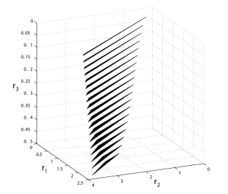
Figure 5: The set of all Schur-stable polygons

V-C Example: (cont)

Having identified the stable intervals, griding of parameter $r_{3}$ yields stable slices, which compose the $3-$D stability region. E.g. Fig. 5 shows the whole region in $(r_{1},r_{2},r_{3})-$ parameter space of three-term controllers, (32), which stabilize the plant (31).

VI Conclusion

The problem of finding the set of all PID and three-term stabilizers for a linear discrete-time system is treated in this paper. The basic result is the transfer and generalization of the counterpart theory of continuous-time PID stabilizers to time-discrete domain. The design method is based on the fact that controller parameters in a linearly transformed parameter space appear decoupled at singular frequencies. Thereby the design problem decouples into detection of stable polygons and assertion of intervals where such polygons may exist. A new simple and powerful rule is introduced to discriminate such intervals. The design method for simultaneous stabilization of several operating points becomes feasible by intersecting convex polygons.

References

- [1] Bajcinca, N.: Design of robust PID controllers using decoupling at singular frequencies, acc. in Automatica, 2006.
- [2] Ho, M.T. , A. Datta and S. P. Bhattacharryya: Structure and synthesis of PID controllers, Springer, 2000 London.
- [3] Munro, N, M.T. Soylemez: Fast calculation of stabilizing PID controllers for uncertain parameter systems, In Proceed. ROCOND 2000, Prague.
- [4] Soylemez, M.T., N. Munro and H. Baki: Fast calculation of stabilizing PID controllers, Automatica 39, 121-126.
- [5] Ackermann, J., D. Kaesbauer and N. Bajcinca: Discrete-time robust PID and Three-Term control, XV IFAC World Congress, 2002 Barcelona.
- [6] Ackermann, J. and D. Kaesbauer: Design of robust PID controllers, Proc. European Control Conference, 2001 Porto.
- [7] Bajcinca, N.: The method of singular frequencies for robust design in an affine parameter space, 9th Mediterranean Conference on Control and Automation, 2001 Dubrovnik.