Incremental Algorithms for Network Management and Analysis based on Closeness Centrality

Abstract

Analyzing networks requires complex algorithms to extract meaningful information. Centrality metrics have shown to be correlated with the importance and loads of the nodes in network traffic. Here, we are interested in the problem of centrality-based network management. The problem has many applications such as verifying the robustness of the networks and controlling or improving the entity dissemination. It can be defined as finding a small set of topological network modifications which yield a desired closeness centrality configuration. As a fundamental building block to tackle that problem, we propose incremental algorithms which efficiently update the closeness centrality values upon changes in network topology, i.e., edge insertions and deletions. Our algorithms are proven to be efficient on many real-life networks, especially on small-world networks, which have a small diameter and a spike-shaped shortest distance distribution. In addition to closeness centrality, they can also be a great arsenal for the shortest-path-based management and analysis of the networks. We experimentally validate the efficiency of our algorithms on large networks and show that they update the closeness centrality values of the temporal DBLP-coauthorship network of 1.2 million users 460 times faster than it would take to compute them from scratch. To the best of our knowledge, this is the first work which can yield practical large-scale network management based on closeness centrality values.

1 Introduction

Centrality metrics, such as closeness or betweenness, quantify how central a node is in a network. They have been successfully used to carry analysis for various purposes such as structural analysis of knowledge networks [23, 26], power grid contingency analysis [14], quantifying importance in social networks [20], analysis of covert networks [16], decision/action networks [5], and even for finding the best store locations in cities [25]. Several works which have been conducted to rapidly compute these metrics exist in the literature. The algorithm with the best asymptotic complexity to compute centrality metrics [2] is believed to be asymptotically optimal [15]. Research have focused on either approximation algorithms for computing centrality metrics [3, 8, 21] or on high performance computing techniques [18, 27]. Today, it is common to find large networks, and we are always in a quest for better techniques which help us while performing centrality-based analysis on them.

When the network topology is modified, ensuring the correctness of the centralities is a challenging task. This problem has been studied for dynamic and streaming networks [10, 17]. Even for some applications involving a static network such as the contingency analysis of power grids and robustness evaluation of networks, to be prepared and take proactive measures, we need to know how the centrality values change when the network topology is modified by an adversary and outer effects such as natural disasters.

A similar problem arises in network management for which not only knowing but also setting the centrality values in a controlled manner via topology modifications is of concern to speed-up or contain the entity dissemination. The problem is hard: there are $m$ candidate edges to delete and $\mathcal{O}(n^{2})$ candidate edges to insert where $n$ and $m$ are the number of nodes and edges in the network, respectively. Here, the main motivation can be calibrating the importance/load of some or all of the vertices as desired, matching their loads to their capacities, boosting the content spread, or making the network immune to adversarial attacks. Similar problems, such as finding the most cost-effective way which reduces the entity dissemination ability of a network [24] or finding a small set of edges whose deletion maximizes the shortest-path length [13], have been investigated in the literature. The problem recently regained a lot of attention: A generic study which uses edge insertions and deletions is done by Tong et al. [28]. They use the changes on the leading eigenvalue to control/speed-up the dissemination process. Other recent works investigate edge insertions to minimize the average shortest path distance [22] or to boost the content spread [4]. From the centrality point of view, there exist studies which focus on maximizing the centrality of a node set [9, 12] or a single node [12] by edge insertions. In generic centrality-based network management problem, the desired centralities of all the nodes need to be obtained or approximated with a small set of topology modifications. As Figure 1 shows, the effect of a local topology modification is usually global. Furthermore, existing algorithms for incremental centrality computation are not efficient enough to be used in practice. Thus, novel incremental algorithms are essential to quickly evaluate the effects of topology modifications on centrality values.

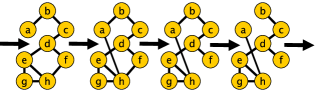
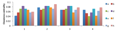
Figure 1: A toy network with nine nodes, three consecutive edge ($ah$, $fh$, and $ab$, respectively) insertions/deletions, and values of closeness centrality.

Our contributions can be summarized as follows:

1. To attack the variants of the centrality-based network management problem, we propose incremental algorithms which efficiently update the closeness centralities upon edge insertions and deletions.

2. The proposed algorithms can serve as a fundamental building block for other shortest-path-based network analyses such as the temporal analysis on the past network data, maintaining centrality on streaming networks, or minimizing/maximizing the average shortest-path distance via edge insertions and deletions.

3. Compared with the existing algorithms, our algorithms have a low-memory footprint making them practical and applicable to very large graphs. For random edge insertions/deletions to the Wikipedia users’ communication graph, we reduced the centrality (re)computation time from 2 days to 16 minutes. And for the real-life temporal DBLP coauthorship network, we reduced the time from 1.3 days to 4.2 minutes.

4. The proposed techniques can easily be adapted to algorithms for approximating centralities. As a result, one can employ a more accurate and faster sampling and obtain better approximations.

The rest of the paper is organized as follows: Section 2 introduces the notation and formally defines the closeness centrality metric. Section 3 defines network management problems we are interested. Our algorithms explained in detail in Section 4. Existing approaches are described in Section 5 and the experimental analysis is given in Section 6. Section 7 concludes the paper.

2 Background

Let $G=(V,E)$ be a network modeled as a simple graph with $n=|V|$ vertices and $m=|E|$ edges where each node is represented by a vertex in $V$, and a node-node interaction is represented by an edge in $E$. Let $\Gamma_{G}(v)$ be the set of vertices which are connected to $v$ in $G$.

A graph $G^{\prime}=(V^{\prime},E^{\prime})$ is a subgraph of $G$ if $V^{\prime}\subseteq V$ and $E^{\prime}\subseteq E$. A path is a sequence of vertices such that there exists an edge between consecutive vertices. A path between two vertices $s$ and $t$ is denoted by $s\leadsto t$ (we sometimes use $s\stackrel{{\scriptstyle P}}{{\leadsto}}t$ to denote a specific path $P$ with endpoints $s$ and $t$). Two vertices $u,v\in V$ are connected if there is a path from $u$ to $v$. If all vertex pairs are connected we say that $G$ is connected. If $G$ is not connected, then it is disconnected and each maximal connected subgraph of $G$ is a connected component, or a component, of $G$. We use ${d}_{G}(u,v)$ to denote the length of the shortest path between two vertices $u,v$ in a graph $G$. If $u=v$ then ${d}_{G}(u,v)=0$. And if $u$ and $v$ are disconnected, then ${d}_{G}(u,v)=\infty$.

Given a graph $G=(V,E)$, a vertex $v\in V$ is called an articulation vertex if the graph $G-v$ (obtained by removing $v$) has more connected components than $G$. Similarly, an edge $e\in E$ is called a bridge if $G-e$ (obtained by removing $e$ from $E$) has more connected components than $G$. $G$ is biconnected if it is connected and it does not contain an articulation vertex. A maximal biconnected subgraph of $G$ is a biconnected component.

2.1 Closeness Centrality

Given a graph $G$, the farness of a vertex $u$ is defined as

$${\tt far}[u]=\sum_{\stackrel{{\scriptstyle v\in V}}{{{d}_{G}(u,v)\neq\infty}}}{d}_{G}(u,v).$$

And the closeness centrality of $u$ is defined as

$${\tt cc}[u]=\frac{1}{{\tt far}[u]}.$$ (1)

If $u$ cannot reach any vertex in the graph ${\tt cc}[u]=0$.

For a sparse unweighted graph $G\ (V,E)$ with $|V|=n$ and $|E|=m$, the complexity of cc computation is $\mathcal{O}(n(m+n))$. For each vertex $s$, Algorithm 1 executes a Single-Source Shortest Paths (SSSP) algorithm. It initiates a breadth-first search (BFS) from $s$, computes the distances to the other vertices, compute ${\tt far}[s]$, the sum of the distances which are different than $\infty$. And, as the last step, it computes ${\tt cc}[s]$. Since a BFS takes $\mathcal{O}(m+n)$ time, and $n$ SSSPs are required in total, the complexity follows.

Data: ${G=(V,E)}$

Output: $cc[.]$

1 for each $s\in V$ do

       $\triangleright$SSSP($G$, $s$) with centrality computation

       $Q\leftarrow$ empty queue

       ${d}[v]\leftarrow\infty,\forall v\in V\setminus{\{s\}}$

       $Q$.push($s$), ${d}[s]\leftarrow 0$

       ${\tt far}[s]\leftarrow 0$

       while $Q$ is not empty do

             $v\leftarrow Q$.pop()

             for all $w\in\Gamma(v)$ do

                   if ${d}[w]=\infty$ then

                         $Q$.push($w$)

                         ${d}[w]\leftarrow{d}[v]+1$

                         ${\tt far}[s]\leftarrow{\tt far}[s]+{d}[w]$

                        

                  

            

       ${\tt cc}[s]=\frac{1}{{\tt far}[s]}$

return ${\tt cc}[.]$

Algorithm 1 CC: Basic centrality computation

3 Problem Definitions

The following problem can be considered as a generalized version of the problems investigated in [9, 12].

Definition 3.1

(Centrality-based network management) Let $G=(V,E)$ be a graph. Given a centrality metric $\cal C$, a target centrality vector ${\mathbf{c}}^{\prime}$, and an upper bound $U$ on the number of inserted/deleted edges, construct a graph $G^{\prime}=(V,E^{\prime})$, s.t., $|E\Delta E^{\prime}|\leq U$ and $||{\mathbf{c}}^{\prime}-{\mathbf{c}}_{G^{\prime}}||$ is minimized.

In this work, we are interested in the closeness metric which is based on shortest paths. Hence, implicitly, we are also interested in the following problem partly investigated in [13, 22, 24].

Definition 3.2

(Shortest-path-based network management) Let $G=(V,E)$ be a graph. Given an upper bound $U$ on the number of inserted/deleted edges, construct a graph $G^{\prime}=(V,E^{\prime})$ where $|E\Delta E^{\prime}|\leq U$ and the (average) shortest-path in $G^{\prime}$ is minimized/maximized.

These problems and their variants have several applications such as slowing down pathogen outbreaks, increasing the efficiency of the advertisements, and analyzing the robustness of a network. Consider an airline company with flights to thousands of airports and aim to add some new routes to increase the load of some underutilized airports. When a new route is inserted, in order to evaluate its overall impact, all the airport centralities need to be re-computed which is a quite expensive task. Hence, we need to have efficient incremental algorithms to tackle this problem. Such algorithms can be used as a fundamental building block to centrality- and shortest-path-based network management problems (and their variants) as well as temporal centrality/shortest-path analyses and dynamic network analyses. In this work, we investigate this subproblem.

Definition 3.3

(Incremental closeness centrality) Given a graph $G=(V,E)$, its centrality vector ${\tt cc}$, and an edge $uv$, find the centrality vector ${\tt cc}^{\prime}$ of the graph $G^{\prime}=(V,E\cup\{uv\})$ (or $G^{\prime}=(V,E\setminus\{uv\})$).

4 Maintaining Centrality

Many interesting real-life networks are scale free. The diameters of these networks grow proportional to the logarithm of the number of nodes. That is, even with hundreds of millions of vertices, the diameter is small, and when the graph is modified with minor updates, it tends to stay small. Combining this with their power-law degree distribution, we obtain the spike-shaped shortest-distance distribution as shown in Figure 3. We use two main approaches: work filtering and SSSP hybridization to exploit these observations and reduce the centrality computation time.

4.1 Work Filtering

For efficient maintenance of closeness centrality in case of an edge insertion/deletion, we propose a work filter which reduces the number of SSSPs in Algorithm 1 and the cost of each SSSP. Work filtering uses three techniques: filtering with level differences, with biconnected component decomposition, and with identical vertices.

4.1.1 Filtering with level differences

The motivation of level-based filtering is detecting the unnecessary updates and filtering them. Let $G=(V,E)$ be the current graph and $uv$ be an edge to be inserted to $G$. Let $G^{\prime}=(V,E\cup{uv})$ be the updated graph. The centrality definition in (1) implies that for a vertex $s\in V$, if ${d}_{G}(s,t)={d}_{G^{\prime}}(s,t)$ for all $t\in V$ then ${\tt cc}[s]={\tt cc}^{\prime}[s]$. The following theorem is used to detect such vertices and filter their SSSPs.

Theorem 4.1

Let $G=(V,E)$ be a graph and $u$ and $v$ be two vertices in $V$ s.t. $uv\notin E$. Let $G^{\prime}=(V,E\cup{uv})$. Then ${\tt cc}[s]={\tt cc}^{\prime}[s]$ if and only if $|{d}_{G}(s,u)-{d}_{G}(s,v)|\leq 1$.

Proof 4.2.

If $s$ is disconnected from $u$ and $v$, $uv$’s insertion will not change the closeness centrality of $s$. Hence, ${\tt cc}[s]={\tt cc}^{\prime}[s]$. If $s$ is only connected to one of $u$ and $v$ in $G$ the difference $|{d}_{G}(s,u)-{d}_{G}(s,v)|$ is $\infty$, and the closeness centrality score of $s$ needs to be updated by using the new, larger connected component containing $s$.

When $s$ is connected to both $u$ and $v$ in $G$, we investigate the edge insertion in three cases as shown in Figure 2:

Case 1. ${d}_{G}(s,u)={d}_{G}(s,v)$: Assume that the path $s\stackrel{{\scriptstyle P}}{{\leadsto}}u$–$v\stackrel{{\scriptstyle P^{\prime}}}{{\leadsto}}t$ is a shortest $s\leadsto t$ path in $G^{\prime}$ containing $uv$. Since ${d}_{G}(s,u)={d}_{G}(s,v)$ there exist another path $s\stackrel{{\scriptstyle P^{\prime\prime}}}{{\leadsto}}v\stackrel{{\scriptstyle P^{\prime}}}{{\leadsto}}t$ in $G^{\prime}$ with one less edge. Hence, $uv$ cannot be in a shortest path: $\forall t\in V,{d}_{G}(s,t)={d}_{G^{\prime}}(s,t)$.

Case 2. $|{d}_{G}(s,u)-{d}_{G}(s,v)|=1$: Let ${d}_{G}(s,u)<{d}_{G}(s,v)$ and assume that $s\stackrel{{\scriptstyle P}}{{\leadsto}}u$–$v\stackrel{{\scriptstyle P^{\prime}}}{{\leadsto}}t$ is a shortest path in $G^{\prime}$ containing $uv$. Since ${d}_{G}(s,v)={d}_{G}(s,u)+1$, there exist another path $s\stackrel{{\scriptstyle P^{\prime\prime}}}{{\leadsto}}v\stackrel{{\scriptstyle P^{\prime}}}{{\leadsto}}t$ in $G^{\prime}$ with the same number of edges. Hence, $\forall t\in V,{d}_{G}(s,t)={d}_{G^{\prime}}(s,t)$.

Case 3. $|{d}_{G}(s,u)-{d}_{G}(s,v)|>1$: Let ${d}_{G}(s,u)<{d}_{G}(s,v)$. The path $s\leadsto u$–$v$ in $G^{\prime}$ is shorter than the shortest $s\leadsto v$ path in $G$ since ${d}_{G}(s,v)>{d}_{G}(s,u)+1$. Hence, an update on ${\tt cc}[s]$ is necessary.

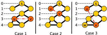
Figure 2: (1) Three cases of edge insertion: when an edge $uv$ is inserted to the graph $G$, for each vertex $s$, one of them is true: (a) ${d}_{G}(s,u)={d}_{G}(s,v)$, (b) $|{d}_{G}(s,u)-{d}_{G}(s,v)|=1$, and (c) $|{d}_{G}(s,u)-{d}_{G}(s,v)|>1$.

Although Theorem 4.1 yields to a filter only in case of edge insertions, the following corollary which is used for edge deletion easily follows.

Corollary 4.3.

Let $G=(V,E)$ be a graph and $u$ and $v$ be two vertices in $V$ s.t. $uv\in E$. Let $G^{\prime}=(V,E\setminus\{uv\})$. Then ${\tt cc}[s]={\tt cc}^{\prime}[s]$ if and only if $|{d}_{G^{\prime}}(s,u)-{d}_{G^{\prime}}(s,v)|\leq 1$.

With this corollary, the work filter can be implemented for both edge insertions and deletions. The pseudocode of the update algorithm in case of an edge insertion is given in Algorithm 2. When an edge $uv$ is inserted/deleted, to employ the filter, we first compute the distances from $u$ and $v$ to all other vertices. And, it filters the vertices satisfying the statement of Theorem 4.1.

Data: ${G=(V,E)}$, ${\tt cc}[.]$, $uv$

Output: ${\tt cc}^{\prime}[.]$

$G^{\prime}\leftarrow(V,E\cup\{uv\})$

${d}u[.]\leftarrow$ SSSP($G$, $u$) $\triangleright$ distances from $u$ in $G$

${d}v[.]\leftarrow$ SSSP($G$, $v$) $\triangleright$ distances from $v$ in $G$

for each $s\in V$ do

       if $|{d}u[s]-{d}v[s]|\leq 1$ then

             ${\tt cc}^{\prime}[s]={\tt cc}[s]$

            

       else

             $\triangleright$ use the computation in Algorithm 1 with $G^{\prime}$

            

      

return ${\tt cc}^{\prime}[.]$

Algorithm 2 Simple work filtering

In theory, filtering by levels can reduce the update time significantly. However, in practice, its effectiveness depends on the underlying structure of $G$. Many real-life networks have been repeatedly shown to possess unique characteristics such as a small diameter and a power-law degree distribution [19]. And the spread of information is extremely fast [6, 7]. The proposed filter exploits one of these characteristics for efficient closeness centrality updates: the distribution of shortest-path lengths. Its efficiency is based on the phenomenon shown in Figure 3 for a set of graphs used in our experiments: the probability distribution function for a shortest-path length being equal to $x$ is unimodular and spike-shaped for many social networks and also some others. This is the outcome of the short diameter and power-law degree distribution. On the other hand, for some spatial networks such as road networks, there are no sharp peaks and the shortest-path distances are distributed in a more uniform way. The work filter we propose here prefer the former.

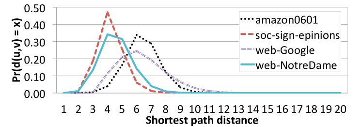
Figure 3: Probability of the distance between two (connected) vertices is equal to $x$ for four social and web networks.

4.1.2 Filtering with biconnected components

Our work filter can be enhanced by employing and maintaining a biconnected component decomposition (BCD) of $G=(V,E)$. A BCD is a partitioning $\Pi$ of the edge set $E$ where $\Pi(e)$ indicates the component of each edge $e\in E$. A toy graph and its BCDs before and after edge insertions are given in Figure 4.

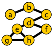
(a) $G$

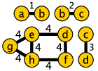
(b) $\Pi$

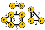
(c) $\Pi^{\prime}$

Figure 4: A graph $G$ (left), its biconnected component decomposition $\Pi$ into $4$ components (middle), and the updated $\Pi^{\prime}$ with $3$ components when the edge $bd$ is inserted (right). The sets of articulation vertices before and after the edge insertion are $\{b,c,d\}$ and $\{b,d\}$, respectively. After the edge addition, $cid=2$. That is to say, the second component contains the new edge. Hence, the biconnected component $2$ is extracted first and executes an update algorithm only for the vertices $\{b,c,d\}$. It also initiates a fixing phase to update the closeness centrality values for the rest of the vertices. After the edge insertion, ${rep}[a]=b$, and ${rep}[e]={rep}[f]={rep}[g]={rep}[h]=b$. Hence, ${\tt R}[b]=2$, ${\tt R}[c]=1$, and ${\tt R}[d]=5$. And, ${\tt RF}[b]=1$, ${\tt RF}[c]=0$, and ${\tt RF}[d]=6$.

When $uv$ is inserted to $G=(V,E)$ and $G^{\prime}=(V,E^{\prime}\cup\{uv\})$ is obtained, we check if

$$\{\Pi(uw):w\in\Gamma_{G}(u)\}\cap\{\Pi(vw):w\in\Gamma_{G}(v)\}$$

is empty or not. If the intersection is not empty, there will be only one element in it, $cid$, which is the id of the biconnected component of $G^{\prime}$ containing $uv$ (otherwise $\Pi$ is not a valid BCD). In this case, $\Pi^{\prime}(e)$ is set to $\Pi(e)$ for all $e\in E$ and $\Pi^{\prime}(uv)$ is set to $cid$. If there is no biconnected component containing both $u$ and $v$ (see Figure 4(c)), i.e., if the intersection above is empty, we construct $\Pi^{\prime}$ from scratch and set $cid=\Pi^{\prime}(uv)$. $\Pi$ can be computed in linear, $\mathcal{O}(m+n)$ time [11]. Hence, the cost of BCD maintenance is negligible compared to the cost of updating closeness centrality.

Let $G^{\prime}_{cid}=(V_{cid},E^{\prime}_{cid})$ be the biconnected component of $G^{\prime}$ containing $uv$ where

$$V_{cid} =\{v\in V:cid\in\{\Pi^{\prime}(vw):vw\in E^{\prime}\}\},$$

$$E^{\prime}_{cid} =\{e\in E^{\prime}:\Pi^{\prime}(e)=cid\}.$$

Let ${\cal A}_{cid}\subseteq V_{cid}$ be the set of articulation vertices in $G^{\prime}_{cid}$. Given $\Pi^{\prime}$, it is easy to detect the articulation vertices since $u$ is an articulation vertex if and only if it is part of at least two components in the BCD: $|\{\Pi^{\prime}(uw):uw\in E^{\prime}\}|>1$.

We will execute SSSPs only for the vertices in $G^{\prime}_{cid}$ and use the new values to fix the centralities for the rest of the graph. The contributions of the vertices in $V\setminus V_{cid}$ are integrated to the SSSPs by using a representative function ${rep}:V\rightarrow V_{cid}\cup\{\tt{null}\}$ which maps each vertex $v\in V$ either to a representative in $G^{\prime}_{cid}$ or to $\tt{null}$ (if $v$ and the vertices in $V_{cid}$ are in different connected components of $G^{\prime}$).

For each vertex $u\in V_{cid}$, we set ${rep}[u]=u$. For the other vertices, let $\overline{G^{\prime}_{cid}}=\{V,E^{\prime}\setminus E^{\prime}_{cid}\}$. If a vertex $v\in V\setminus V_{cid}$ and an articulation vertex $u\in{\cal A}_{cid}$ are connected in $\overline{G^{\prime}_{cid}}$, i.e., ${d}_{\overline{G^{\prime}_{cid}}}(u,v)\neq\infty$, we say that $v$ is represented by $u$ in $G^{\prime}_{cid}$ and set ${rep}[v]=u$. Otherwise, ${rep}[v]$ is set to ${\tt null}$. The following theorem states that ${rep}$ is well defined: each vertex is represented by at most one vertex.

Theorem 4.4.

For each $v$ in $V\setminus V_{cid}$, there is at most one articulation vertex $u\in{\cal A}_{cid}$ such that ${d}_{\overline{G^{\prime}_{cid}}}(u,v)\neq\infty$.

Proof 4.5.

The proof directly follows from the definition of BCD and is omitted.

Since all the (shortest) paths from a vertex $v\in V\setminus V_{cid}$ to a vertex in $V_{cid}$ are passing through ${rep}[v]$, the following is a corollary of the theorem.

Corollary 4.6.

For each vertex $v\in V\setminus V_{cid}$ with ${rep}[v]\neq{\tt null}$, ${d}_{\overline{G^{\prime}_{cid}}}(v,{rep}[v])={d}_{G^{\prime}}(v,{rep}[v]),$ which is different than $\infty$. Furthermore, for a vertex $w\in V$ which is also represented in $G^{\prime}_{cid}$ but not in the connected component of ${\overline{G^{\prime}_{cid}}}$ containing $v$, ${d}_{G^{\prime}}(v,w)$ is equal to

$${d}_{G^{\prime}}(v,{rep}[v])+{d}_{G^{\prime}}({rep}[v],{rep}[w])+{d}_{G^{\prime}}({rep}[w],w).$$

If $w\in V_{cid}$ the last term on the right is $0$, since ${rep}[w]=w$.

To correctly update the new centrality values, we compute two extra values for each vertex $u\in V_{cid}$,

$${\tt R}[u] =\left|\{v\in V:{rep}[v]=u\}\right|,$$ (2)

$${\tt RF}[u] =\sum_{\stackrel{{\scriptstyle v\in V}}{{{rep}[v]=u}}}{d}_{G^{\prime}}(u,v).$$ (3)

That is, ${\tt R}[u]$ is the number of vertices in $V$ which are represented by $u$ (including $u$). And ${\tt RF}[u]$ is the farness of $u$ to these vertices in $G^{\prime}$. The modified update algorithm is given in Algorithm 3.

Data: ${G=(V,E)}$, $\Pi$, ${\tt cc}$, ${\tt far}$, $uv$

Output: ${\tt cc}^{\prime}[.]$, ${\tt far}^{\prime}[.]$

1 $\triangleright$ prepare for filtering

$G^{\prime}\leftarrow(V,E^{\prime})$ where $E^{\prime}\leftarrow E\cup\{uv\}$

$cSet_{u}\leftarrow\{\Pi(uw):w\in\Gamma_{G}(u)\}$

$cSet_{v}\leftarrow\{\Pi(vw):w\in\Gamma_{G}(v)\}$

if $cSet_{u}\cap cSet_{v}\neq\emptyset$ then

       $cid\leftarrow$ #the common component

       $\Pi^{\prime}(e)\leftarrow\Pi(e)$ $\forall e\in E$, $\Pi^{\prime}(uv)\leftarrow cid$

      

else  construct $\Pi^{\prime}$ from $G^{\prime}$, $cid\leftarrow\Pi^{\prime}(uv)$

$V_{cid}\leftarrow\{v\in V:cid\in\{\Pi^{\prime}(vw):vw\in E^{\prime}\}\}$

$E^{\prime}_{cid}\leftarrow\{e\in E^{\prime}:\Pi^{\prime}(e)=cid\}$

$G^{\prime}_{cid}=(V_{cid},E^{\prime}_{cid})$

$G_{cid}=(V_{cid},E^{\prime}_{cid}\setminus\{uv\})$

Set ${rep}[v]$, $\forall v\in V$

${\tt R}[u]\leftarrow\left|\{v\in V,{rep}[v]=u\}\right|$, $\forall u\in V_{cid}$

${\tt RF}[u]\leftarrow\sum_{v\in V,{rep}[v]=u}{d}_{G^{\prime}}(u,v)$, $\forall u\in V_{cid}$

${d}u[.]\leftarrow$ SSSP($G_{cid}$, $u$), ${d}v[.]\leftarrow$ SSSP($G_{cid}$, $v$)

2$\triangleright$ update phase

for each $s\in V_{cid}$ do

       if $|{d}u[s]-{d}v[s]|\leq 1$ then ${\tt cc}^{\prime}[s]={\tt cc}[s]$

       else

            3 $Q\leftarrow$ empty queue

             ${d}[v]\leftarrow\infty$, $\forall v\in V_{cid}\setminus{\{s\}}$

             $Q$.push($s$), ${d}[s]\leftarrow 0$

             ${\tt far}^{\prime}[s]\leftarrow 0$

             while $Q$ is not empty do

                   $v\leftarrow Q$.pop()

                   for all $w\in\Gamma_{G^{\prime}_{cid}}(v)$ do

                         if ${d}[w]=\infty$ then

                               $Q$.push($w$)

                               ${d}[w]\leftarrow{d}[v]+1$

                              4 ${\tt far}^{\prime}[s]\leftarrow{\tt far}^{\prime}[s]+({d}[w]\times{\tt R}[w])+{\tt RF}[w]$

                              

                        

                  

             ${\tt cc}^{\prime}[s]=\frac{1}{{\tt far}^{\prime}[s]}$

      

5$\triangleright$ fix phase

for each $v\in V\setminus V_{cid}$ do

       $r\leftarrow{rep}[v]$

       if $r\neq{\tt{null}}$ and ${\tt far}[r]\neq{\tt far}^{\prime}[r]$ then

            6 ${\tt far}^{\prime}[v]\leftarrow{\tt far}[v]-({\tt far}[r]-{\tt far}^{\prime}[r])$

             ${\tt cc}^{\prime}[v]\leftarrow\frac{1}{{\tt far}^{\prime}[v]}$

            

      

return ${\tt cc}^{\prime}[.]$

Algorithm 3 Update with BCD and level differences

Lemma 4.7.

For each vertex $v\in V_{cid}$, Algorithm 3 computes the correct ${\tt cc}^{\prime}[v]$ value.

Proof 4.8.

We will prove that ${\tt far}^{\prime}[v]$ is correct for all $v\in V_{cid}$. Let $v=s$ be the vertex whose closeness centrality update is started at line 3. At line 3 of Algorithm 3, the update on ${\tt far}^{\prime}[v]$ is ${d}_{G^{\prime}}(v,w)\times{\tt R}[w]+{\tt RF}[w]$ which can be rewritten as

$$\sum_{\stackrel{{\scriptstyle u\in V}}{{{rep}[u]=w}}}{d}_{G^{\prime}}(v,w)+{d}_{G^{\prime}}(w,u),$$

by using (2) and (3). According to Corollary 4.6, this is equal to

$$\sum_{\stackrel{{\scriptstyle u\in V}}{{{rep}[u]=w}}}{d}_{G^{\prime}}(v,u).$$

Due to the definition of ${rep}$, only the vertices which are connected to $v$ will have an effect on ${\tt far}^{\prime}[v]$. And due to Theorem 4.4, each vertex can contribute to at most one update. Hence

$$\sum_{w\in V_{cid}}\sum_{\stackrel{{\scriptstyle u\in V}}{{{rep}[u]=w}}}{d}_{G^{\prime}}(v,u)=\sum_{\stackrel{{\scriptstyle u\in V}}{{{d}_{G^{\prime}}(v,u)\neq\infty}}}{d}_{G^{\prime}}(v,u),$$

which is the ${\tt far}^{\prime}[v]$ in $G^{\prime}$ as desired.

Lemma 4.9.

For each vertex $v\in V\setminus V_{cid}$, Algorithm 3 computes the correct ${\tt cc}^{\prime}[v]$ value.

Proof 4.10.

We will prove that ${\tt far}^{\prime}[v]$ is correct for all $v\in V\setminus V_{cid}$ after the fix phase. Let $u={rep}[v]$. If $u$ is null then $v$’s farness and hence closeness value will remain the same.

Assume that $u$ is not null. Let $w$ be a vertex with ${rep}[w]\neq{\tt null}$. If $w$ and $v$ are in the same connected component of $\overline{G^{\prime}_{cid}}$ then ${d}_{G}(v,w)={d}_{G^{\prime}}(v,w)$ and ${d}_{G}(u,w)={d}_{G^{\prime}}(u,w)$. Hence, the change on ${\tt far}[v]$ and ${\tt far}[u]$ due to $w$ are both $0$. On the other hand, if $w$ is in a different connected component of $\overline{G^{\prime}_{cid}}$ according to Corollary 4.6,

$${d}_{G^{\prime}}(v,w)={d}_{G^{\prime}}(v,u)+{d}_{G^{\prime}}(u,{rep}[w])+{d}_{G^{\prime}}({rep}[w],w),$$

where the sum of the second and the third terms is equal to ${d}_{G^{\prime}}(u,w)$. Since the first term does not change by the insertion of $uv$, the change on ${d}_{G^{\prime}}(u,w)$ is equal to the change on ${d}_{G^{\prime}}(v,w)$. That is when aggregated, the change on ${\tt far}[v]$ is equal to the change on ${\tt far}[u]$. Lemma 4.7 implies that ${\tt far}[u]$ is correct. Hence, ${\tt far}^{\prime}[v]$, computed at line 3, must also be correct.

Theorem 4.11.

For each vertex $v\in V$, Algorithm 3 computes the correct ${\tt cc}^{\prime}[v]$ value.

Proof 4.12.

Follows from Lemma 4.7 and 4.9.

The complexity of the update algorithm is $\mathcal{O}(n(m+n))$. And the overhead of filter preparation (line 3 through 3) is $\mathcal{O}(m+n)$ since it only contains a constant number of graph traversals. In case of an edge deletion, it is enough to get $G^{\prime}_{cid}$ as the biconnected component which was containing the deleted edge. The rest of the procedure can be adapted in a straightforward manner.

4.1.3 Filtering with identical vertices

Our preliminary analyses on various networks show that some of the graphs contain a significant amount of identical vertices which have the same/a similar neighborhood structure. This can be exploited to reduce the number of SSSPs further. We investigate two types of identical vertices.

Definition 4.13.

In a graph $G$, two vertices $u$ and $v$ are type-I-identical if and only if $\Gamma_{G}(u)=\Gamma_{G}(v)$.

Definition 4.14.

In a graph $G$, two vertices $u$ and $v$ are type-II-identical if and only if $\{u\}\cup\Gamma_{G}(u)=\{v\}\cup\Gamma_{G}(v)$.

Both types form an equivalance class relation since they are reflexive, symmetric, and transitive. Furthermore, all the non-trivial classes they form (i.e., the ones containing more than one vertex) are disjoint.

Let $u,v\in V$ be two identical vertices. One can see that for any vertex $w\in V\setminus\{u,v\}$, ${d}_{G}(u,w)={d}_{G}(v,w)$. Then the following is true.

Corollary 4.15.

Let ${\cal I}\subseteq V$ be a vertex-class containing type-I or type-II identical vertices. Then the closeness centrality values of all the vertices in ${\cal I}$ are equal.

To construct these equivalance classes for the initial graph, we first use a hash function to map each vertex neighborhood to an integer: $hash_{I}[u]=\sum_{v\in\Gamma_{G}(u)}v$. We then sort the vertices with respect to their hash values and construct the type-I vertex-classes by eliminating false positives due to collisions on the hash function. A similar process is applied to detect type-II vertex classes. The complexity of this initial construction is $\mathcal{O}(n\log n+m)$ assuming the number of collisions is small and hence, false-positive detection cost is negligible.

Maintaining the equivalance classes in case of edge insertions and deletions is easy: For example, when $uv$ is added to $G$, we first subtract $u$ and $v$ from their classes and insert them to new ones (or leave them as singleton if none of the vertices are now identical with them). The cost of this maintenance is $\mathcal{O}(n+m)$.

While updating closeness centralities of the vertices in $V$, we execute an SSSP at line 3 of Algorithm 3 for at most one vertex from each class. For the rest of the vertices, we use the same closeness centrality value. The improvement is straightforward and the modifications are minor. For brevity, we do not give the pseudocode.

4.2 SSSP Hybridization

The spike-shaped distribution given in Figure 3 can also be exploited for SSSP hybridization. Consider the execution of Algorithm 1: while executing an SSSP with source $s$, for each vertex pair $u,v$, $u$ is processed before $v$ if and only if $d_{G}(s,u)<d_{G}(s,v)$. That is, Algorithm 1 consecutively uses the vertices with distance $k$ to find the vertices with distance $k+1$. Hence, it visits the vertices in a top-down manner. SSSP can also be performed in a a bottom-up manner. That is to say, after all distance (level) $k$ vertices are found, the vertices whose levels are unknown can be processed to see if they have a neighbor at level $k$.

Figure 5 gives the execution times of bottom-up and top-down SSSP variants for processing each level. The trend for top-down resembles the shortest distance distribution in small-world networks. This is expected since in each level $\ell$, the vertices that are $\ell$ step far away from $s$ are processed. On the other hand, for the bottom-up variant, the execution time is decreasing since the number of unprocessed nodes is decreasing. Following the idea of Beamer et al. [1], we hybridize the SSSPs throughout the centrality update phase in Algorithm 3. We simply compare the number of edges need to be processed for each variant and choose the cheaper one. For the case presented in Figure 5, the hybrid algorithm is $3.6$ times faster than the top-down variant.

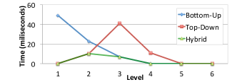
Figure 5: Execution times of bottom-up, top-down, and hybrid SSSPs at each level for the wiki-Talk graph. The hybrid version is $3.63$ and $4.59$ times faster than the top-down and bottom-up versions respectively.

5 Related Work

To the best of our knowledge, there are only two works that deal with maintaining centrality in dynamic networks. Yet, both are interested in betweenness centrality. Lee et al. proposed the QUBE framework which updates betweenness centrality in case of edge insertion and deletion within the network [17]. QUBE relies on the biconnected component decomposition of the graphs. Upon an edge insertion or deletion, assuming that the decomposition does not change, only the centrality values within the updated biconnected component are recomputed from scratch. If the edge insertion/deletion affects the decomposition the modified graph is decomposed into its biconnected components and the centrality values in the affected part are recomputed. The distribution of the vertices to the biconnected components is an important criteria for the performance of QUBE. If a large component exists, which is the case for many real-life networks, one should not expect a significant reduction on update time. Unfortunately, the performance of QUBE is only reported on small graphs (less than 100K edges) with very low edge density. In other words, it only performs significantly well on small graphs with a tree-like structure having many small biconnected components.

Green et al. proposed a technique to update centrality scores rather than recomputing them from scratch upon edge insertions (can be extended to edge deletions) [10]. The idea is storing the whole data structure used by the previous betweenness centrality update kernel. This storage is indeed useful for two main reasons: it avoids a significant amount of recomputation since some of the centrality values will stay the same. And second, it enables a partial traversal of the graph even when an update is necessary. However, as the authors state, $\mathcal{O}(n^{2}+nm)$ values must be kept on the disk. For the Wikipedia user communication and DBLP coauthorship networks, which contain thousands of vertices and millions of edges, the technique by Green et al. requires TeraBytes of memory. The largest graph used in [10] has approximately $20K$ vertices and $200K$ edges; the quadratic storage cost prevents their storage-based techniques to scale any higher. On the other hand, the memory footprint of our algorithms are linear and hence they are much more practical.

6 Experimental Results

We implemented our algorithms in C. The code is compiled with gcc v4.6.2 and optimization flags -O2 -DNDEBUG. The graphs are kept in memory in the compressed row storage (CRS) format. The experiments are run on a computer with two Intel Xeon E$5520$ CPU clocked at $2.27$GHz and equipped with $48$GB of main memory. All the experiments are run sequentially.

For the experiments, we used $10$ networks from the UFL Sparse Matrix Collection and we also extracted the coauthor network from current set of DBLP papers. Properties of the graphs are summarized in Table 1. We symmetrized the directed graphs. The graphs are listed by increasing number of edges and a distinction is made between small graphs (with less than 500K edges) and the large graphs (with more than 500K) edges.

Graph			Time (in sec.)
name	$|V|$	$|E|$	Org.	Best	Speedup
hep-th	8.3K	15.7K	1.41	0.05	29.4
PGPgiantcompo	10.6K	24.3K	4.96	0.04	111.2
astro-ph	16.7K	121.2K	14.56	0.36	40.5
cond-mat-2005	40.4K	175.6K	77.90	2.87	27.2
geometric mean					43.5
soc-sign-epinions	131K	711K	778	6.25	124.5
loc-gowalla	196K	950K	2,267	53.18	42.6
web-NotreDame	325K	1,090K	2,845	53.06	53.6
amazon0601	403K	2,443K	14,903	298	50.0
web-Google	875K	4,322K	65,306	824	79.2
wiki-Talk	2,394K	4,659K	175,450	922	190.1
DBLP-coauthor	1,236K	9,081K	115,919	251	460.8
geometric mean					99.8

Table 1: The graphs used in the experiments. Column Org. shows the initial closeness computation time of CC and Best is the best update time we obtain in case of streaming data.

6.1 Handling topology modifications

To assess the effectiveness of our algorithms, we need to know that when each edge is inserted to/deleted from the graph. Our datasets from UFL Sparse Matrix Collection do not have this information. To conduct our experiments on these datasets, we delete 1,000 edges from a graph chosen randomly in the following way: A vertex $u\in V$ is selected randomly (uniformly), and a vertex $v\in\Gamma_{G}(u)$ is selected randomly (uniformly). Since we do not want to change the connectivity in the graph (having disconnected components can make our algorithms much faster and it will not be fair to CC), we discard $uv$ if it is a bridge. If this is not the case we delete it from $G$ and continue. We construct the initial graph by deleting these 1,000 edges. Each edge is then inserted one by one, and our algorithms are used to recompute the closeness centrality after each insertion. Beside these random insertion experiments, we also evaluated our algorithms on a real temporal dataset of the DBLP coauthor graph. In this graph, there is an edge between two authors if they published a paper. Publication dates are used as timestamps of edges. We first constructed the graph for the papers published before January 1, 2013. Then, we inserted the coauthorship edges of the papers since then. Although our experiments perform edge insertion, edge deletion is a very similar process which should give comparable results.

In addition to CC, we configure our algorithms in four different ways: CC-B only uses biconnected component decomposition (BCD), CC-BL uses BCD and filtering with levels, CC-BLI uses all three work filtering techniques including identical vertices. And CC-BLIH uses all the techniques described in this paper including SSSP hybridization.

Table 2 presents the results of the experiments.The second column, CC, shows the time to run the full Brandes algorithm for computing closeness centrality on the original version of the graph. Columns $3$–$6$ of the table present absolute runtimes (in seconds) of the centrality computation algorithms. The next four columns, $7$–$10$, give the speedups achieved by each configuration. For instance, on the average, updating the closeness values by using CC-B on PGPgiantcompo is $11.5$ times faster than running CC. Finally the last column gives the overhead of our algorithms per edge insertion, i.e., the time necessary to detect the vertices to be updated, and maintain BCD and identical-vertex classes. Geometric means of these times and speedups are also given to provide comparison across instances.

	Time (secs)					Speedups				Filter
Graph	CC	CC-B	CC-BL	CC-BLI	CC-BLIH	CC-B	CC-BL	CC-BLI	CC-BLIH	time (secs)
hep-th	1.413	0.317	0.057	0.053	0.048	4.5	24.8	26.6	29.4	0.001
PGPgiantcompo	4.960	0.431	0.059	0.055	0.045	11.5	84.1	89.9	111.2	0.001
astro-ph	14.567	9.431	0.809	0.645	0.359	1.5	18.0	22.6	40.5	0.004
cond-mat-2005	77.903	39.049	5.618	4.687	2.865	2.0	13.9	16.6	27.2	0.010
Geometric mean	9.444	2.663	0.352	0.306	0.217	3.5	26.8	30.7	43.5	0.003
soc-sign-epinions	778.870	257.410	20.603	19.935	6.254	3.0	37.8	39.1	124.5	0.041
loc-gowalla	2,267.187	1,270.820	132.955	135.015	53.182	1.8	17.1	16.8	42.6	0.063
web-NotreDame	2,845.367	579.821	118.861	83.817	53.059	4.9	23.9	33.9	53.6	0.050
amazon0601	14,903.080	11,953.680	540.092	551.867	298.095	1.2	27.6	27.0	50.0	0.158
web-Google	65,306.600	22,034.460	2,457.660	1,701.249	824.417	3.0	26.6	38.4	79.2	0.267
wiki-Talk	175,450.720	25,701.710	2,513.041	2,123.096	922.828	6.8	69.8	82.6	190.1	0.491
DBLP-coauthor	115,919.518	18,501.147	288.269	251.557	252.647	6.2	402.1	460.8	458.8	0.530
Geometric mean	13,884.152	4,218.031	315.777	273.036	139.170	3.2	43.9	50.8	99.7	0.146

Table 2: Execution times in seconds of all the algorithms and speedups when compared with the basic closeness centrality algorithm CC. In the table CC-B is the variant which uses only BCDs, CC-BL uses BCDs and filtering with levels, CC-BLI uses all three work filtering techniques including identical vertices. And CC-BLIH uses all the techniques described in this paper including SSSP hybridization.

The times to compute closeness centrality using CC on the small graphs range between $1$ to $77$ seconds. On large graphs, the times range from $13$ minutes to $49$ hours. Clearly, CC is not suitable for real-time network analysis and management based on shortest paths and closeness centrality. When all the techniques are used (CC-BLIH), the time necessary to update the closeness centrality values of the small graphs drops below $3$ seconds per edge insertion. The improvements range from a factor of $27.2$ (cond-mat-2005) to $111.2$ (PGPgiantcompo), with an average improvement of $43.5$ across small instances. On large graphs, the update time per insertion drops below $16$ minutes for all graphs. The improvements range from a factor of $42.6$ (loc-gowalla) to $458.8$ (DBLP-coauthor), with an average of $99.7$. For all graphs, the time spent filtering the work is below one second which indicates that the majority of the time is spent for SSSPs. Note that this part is pleasingly parallel since each SSSP is independent from each other.

The overall improvement obtained by the proposed algorithms is very significant. The speedup obtained by using BCDs (CC-B) are $3.5$ and $3.2$ on the average for small and large graphs, respectively. The graphs PGPgiantcompo, and wiki-Talk benefits the most from BCDs (with speedups $11.5$ and $6.8$, respectively). Clearly using the biconnected component decomposition improves the update performance. However, filtering by level differences is the most efficient technique: CC-BL brings major improvements over CC-B. For all social networks, CC-BL increased the performance when compared with CC-B, the speedups range from $4.8$ (web-NotreDame) to $64$ (DBLP-coauthor). Overall, CC-BL brings a $7.61$ improvement on small graphs and a $13.44$ improvement on large graphs over CC.

For each added edge $uv$, let $X$ be the random variable equal to $|{d}_{G}(u,w)-{d}_{G}(v,w)|$. By using 1,000 $uv$ edges, we computed the probabilities of the three cases we investigated before and give them in Fig. 6. For each graph in the figure, the sum of first two columns gives the ratio of the vertices not updated by CC-BL. For the networks in the figure, not even $20\%$ of the vertices require an update ($Pr(X>1)$). This explains the speedup achieved by filtering using level differences. Therefore, level filtering is more useful for the graphs having characteristics similar to small-world networks.

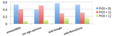
Figure 6: The bars show the distribution of random variable $X=|{d}_{G}(u,w)-{d}_{G}(v,w)|$ into three cases we investigated when an edge $uv$ is added.

Filtering with identical vertices is not as useful as the other two techniques in the work filter. Overall, there is a $1.15$ times improvement with CC-BLI on both small and large graphs compared to CC-BL. For some graphs, such as web-NotreDame and web-Google, improvements are much higher ($30\%$ and $31\%$, respectively).

Finally, the hybrid implementation of SSSP also proved to be useful. CC-BLIH is faster than CC-BLI by a factor of $1.42$ on small graphs and by a factor of $1.96$ on large graphs. Although it seems to improve the performance for all graphs, in some few cases, the performance is not improved significantly. This can be attributed to incorrect decisions on SSSP variant to be used. Indeed, we did not benchmark the architecture to discover the proper parameter. CC-BLIH performs the best on social network graphs with an improvement ratio of $3.18$ (soc-sign-epinions), $2.54$ (loc-gowalla), and $2.30$ (wiki-Talk).

All the previous results present the average update time for 1,000 successively added edges. Hence, they do not say anything about the variance. Figure 7 shows the runtimes of CC-B and CC-BLIH per edge insertion for web-NotreDame in a sorted order. The runtime distribution of CC-B clearly has multiple modes. Either the runtime is lower than $100$ milliseconds or it is around $700$ seconds. We see here the benefit of BCD. According to the runtime distribution, about $59\%$ of web-NotreDame’s vertices are inside small biconnected components. Hence, the time per edge insertion drops from 2,845 seconds to 700. Indeed, the largest component only contains $41\%$ of the vertices and $76\%$ of the edges of the original graph. The decrease in the size of the components accounts for the gain of performance.

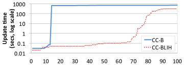
Figure 7: Sorted list of the runtimes per edge insertion for the first $100$ added edges of web-NotreDame.

The impact of level filtering can also be seen on Figure 7. $60\%$ of the edges in the main biconnected component do not change the closeness values of many vertices and the updates that are induced by their addition take less than $1$ second. The remaining edges trigger more expensive updates upon insertion. Within these $30\%$ expensive edge insertions, identical vertices and SSSP hybridization provide a significant improvement (not shown in the figure).

Better Speedups on Real Temporal Data

The best speedups are obtained on the DBLP coauthor network, which uses real temporal data. Using CC-B, we reach $6.2$ speedup w.r.t. CC, which is bigger than the average speedup on all networks. Main reason for this behavior is that $10\%$ of the inserted edges are actually the new vertices joining to the network, i.e., authors with their first publication, and CC-B handles these edges quite fast. Applying CC-BL gives a $64.8$ speedup over CC-B, which is drastically higher than on all other graphs. Indeed, only $0.7\%$ of the vertices require to run a SSSP algorithm when an edge is inserted on the DBLP network. For the synthetic cases, this number is $12\%$. CC-BLI provides similar speedups with random insertions and CC-BLIH does not provide speedups because of the structure of the graph. Overall, speedups obtained with real temporal data reaches $460.8$, i.e., $4.6$ times greater than the average speedup on all graphs. Our algorithms appears to perform much better on real applications than on synthetic ones.

6.2 Summary

All the techniques presented in this paper allow to update closeness centrality faster than the non-incremental algorithm presented in [2] by a factor of $43.5$ on small graphs and $99.7$ on large ones. Small-world networks such as social networks benefit very well from the proposed techniques. They tend to have a biconnected component structure that allow to gain some improvement using CC-B. However, they usually have a large biconnected component and still, most of the gain is derived from exploiting their spike-shaped distance distribution which brings at least a factor of $13.4$. Identical vertices typically brings a small amount of improvement but helps to increase the performance during expensive updates. Using all the techniques, we achieved to reduce the closeness centrality update time from $2$ days to $16$ minutes for the graph with the most vertices in our dataset (wiki-Talk). And for the temporal DBLP coauthorship graph, which has the most edges, we reduced the centrality update time from 1.3 days to 4.2 minutes.

7 Conclusion

In this paper we propose the first algorithms to achieve fast updates of exact centrality values on incremental network modification at such a large scale. Our techniques exploit the biconnected component decomposition of these networks, their spike-shaped shortest-distance distributions, and the existence of nodes with identical neighborhood. In large networks with more than $500K$ edges, our techniques proved to bring a $99$ times speedup in average. With a speedup of 458, the proposed techniques may even allow DBLP to reflect the impact on centrality of the papers published in quasi real-time. Our algorithms will serve as a fundamental building block for the centrality-based network management problem, closeness centrality computations on dynamic/streaming networks, and their temporal analysis.

The techniques presented in this paper can directly be extended in two ways. First, using a statistical sampling to compute an approximation of closeness centrality only requires a minor adaptation on the SSSP kernel to compute the contribution of the source vertex to other vertices instead of its own centrality. Second, the techniques presented here also apply to betweenness centrality with minor adaptations.

As a future work, we plan to investigate local search techniques for the centrality-based network management problem using our incremental centrality computation algorithms.

8 Acknowledgments

This work was supported in parts by the DOE grant DE-FC02-06ER2775 and by the NSF grants CNS-0643969, OCI-0904809, and OCI-0904802.

References

- [1] S. Beamer, K. Asanović, and D. Patterson. Direction-optimizing breadth-first search. In Proc. of Supercomputing, 2012.
- [2] U. Brandes. A faster algorithm for betweenness centrality. Journal of Mathematical Sociology, 25(2):163–177, 2001.
- [3] S. Y. Chan, I. X. Y. Leung, and P. Liò. Fast centrality approximation in modular networks. In Proc. of CIKM-CNIKM, 2009.
- [4] V. Chaoji, S. Ranu, R. Rastogi, and R. Bhatt. Recommendations to boost content spread in social networks. In Proc. of WWW, 2012.
- [5] Ö. Şimşek and A. G. Barto. Skill characterization based on betweenness. In Proc. of NIPS, 2008.
- [6] B. Doerr, M. Fouz, and T. Friedrich. Social networks spread rumors in sublogarithmic time. In Proc. of STOC, 2011.
- [7] B. Doerr, M. Fouz, and T. Friedrich. Why rumors spread so quickly in social networks. Communications of the ACM, 55(6):70–75, June 2012.
- [8] D. Eppstein and J. Wang. Fast approximation of centrality. In Proc. of SODA, 2001.
- [9] M. G. Everett and S. P. Borgatti. Extending centrality. Models and methods in social network analysis, 35(1):57–76, 2005.
- [10] O. Green, R. McColl, and D. A. Bader. A fast algorithm for streaming betweenness centrality. In Proc. of SocialCom, 2012.
- [11] J. Hopcroft and R. Tarjan. Algorithm 447: efficient algorithms for graph manipulation. Communications of the ACM, 16(6):372–378, June 1973.
- [12] V. Ishakian, D. Erdös, E. Terzi, and A. Bestavros. A framework for the evaluation and management of network centrality. In Proc. of SDM, 2012.
- [13] E. Israeli and R. K. Wood. Shortest-path network interdiction. Networks, 40:2002, 2002.
- [14] S. Jin, Z. Huang, Y. Chen, D. G. Chavarría-Miranda, J. Feo, and P. C. Wong. A novel application of parallel betweenness centrality to power grid contingency analysis. In Proc. of IPDPS, 2010.
- [15] S. Kintali. Betweenness centrality : Algorithms and lower bounds. CoRR, abs/0809.1906, 2008.
- [16] V. Krebs. Mapping networks of terrorist cells. Connections, 24, 2002.
- [17] M.-J. Lee, J. Lee, J. Y. Park, R. H. Choi, and C.-W. Chung. QUBE: a Quick algorithm for Updating BEtweenness centrality. In Proc. of WWW, 2012.
- [18] K. Madduri, D. Ediger, K. Jiang, D. A. Bader, and D. G. Chavarría-Miranda. A faster parallel algorithm and efficient multithreaded implementations for evaluating betweenness centrality on massive datasets. In Proc. of IPDPS, 2009.
- [19] M. McGlohon, L. Akoğlu, and C. Faloutsos. Statistical Properties of Social Networks, chapter II in Social Network Data Analytics. Springer, 2011.
- [20] E. L. Merrer and G. Trédan. Centralities: Capturing the fuzzy notion of importance in social graphs. In Proc. of SNS, 2009.
- [21] K. Okamoto, W. Chen, and X.-Y. Li. Ranking of closeness centrality for large-scale social networks. In Proc. of FAW, 2008.
- [22] M. Papagelis, F. Bonchi, and A. Gionis. Suggesting ghost edges for a smaller world. In Proc. of CIKM, 2011.
- [23] M. C. Pham and R. Klamma. The structure of the computer science knowledge network. In Proc. of ASONAM, 2010.
- [24] C. A. Phillips. The network inhibition problem. In Proc. of STOC, 1993.
- [25] S. Porta, V. Latora, F. Wang, E. Strano, A. Cardillo, S. Scellato, V. Iacoviello, and R. Messora. Street centrality and densities of retail and services in Bologna, Italy. Environment and Planning B: Planning and Design, 36(3):450–465, 2009.
- [26] X. Shi, J. Leskovec, and D. A. McFarland. Citing for high impact. In Proc. of JCDL, 2010.
- [27] Z. Shi and B. Zhang. Fast network centrality analysis using GPUs. BMC Bioinformatics, 12:149, 2011.
- [28] H. Tong, B. A. Prakash, T. Eliassi-Rad, M. Faloutsos, and C. Faloutsos. Gelling, and melting, large graphs by edge manipulation. In Proc. of CIKM, 2012.