Abstract

There is increasing interest in broad application areas in defining flexible joint models for data having a variety of measurement scales, while also allowing data of complex types, such as functions, images and documents. We consider a general framework for nonparametric Bayes joint modeling through mixture models that incorporate dependence across data types through a joint mixing measure. The mixing measure is assigned a novel infinite tensor factorization (ITF) prior that allows flexible dependence in cluster allocation across data types. The ITF prior is formulated as a tensor product of stick-breaking processes. Focusing on a convenient special case corresponding to a Parafac factorization, we provide basic theory justifying the flexibility of the proposed prior and resulting asymptotic properties. Focusing on ITF mixtures of product kernels, we develop a new Gibbs sampling algorithm for routine implementation relying on slice sampling. The methods are compared with alternative joint mixture models based on Dirichlet processes and related approaches through simulations and real data applications.

1 INTRODUCTION

There has been considerable recent interest in joint modeling of data of widely disparate types, including not only real numbers, counts and categorical data but also more complex objects, such as functions, shapes, and images. We refer to this general problem as mixed domain modeling (MDM), and major objectives include exploring dependence between the data types, co-clustering, and prediction. Until recently, the emphasis in the literature was almost entirely on parametric hierarchical models for joint modeling of mixed discrete and continuous data without considering more complex object data. The two main strategies are to rely on underlying Gaussian variable models (Muthen, 1984) or exponential family models, which incorporate shared latent variables in models for the different outcomes (Sammel et al., 1997; Dunson, 2000, 2003). Recently, there have been a number of articles using these models as building blocks in discrete mixture models relying on Dirichlet processes (DPs) or closely-related variants (Cai et al., 2011; Song et al., 2009; Yang & Dunson, 2010). DP mixtures for mixed domain modeling were also considered by Hannah et al. (2011); Shahbaba & Neal (2009); Dunson & Bhattacharya (2010) among others. Related approaches are increasingly widely-used in broad machine learning applications, such as for joint modeling of images and captions (Li et al., 2011), and have rapidly become a standard tool for MDM.

Although such joint Dirichlet process mixture models (DPMs) are quite flexible, and can accommodate joint modeling with complicated objects such as functions (Bigelow & Dunson, 2009), they suffer from a key disadvantage in relying on conditional independence given a single latent cluster index. For example, as motivated in Dunson (2009, 2010), the DP and related approaches imply that two subjects $i$ and $i^{\prime}$ are either allocated to the same cluster ($C_{i}=C_{i^{\prime}}$) globally for all their parameters or are not clustered. The soft probabilistic clustering of the DP is appealing in leading to substantial dimensionality reduction, but a single global cluster index conveys several substantial practical disadvantages. Firstly, to realistically characterize joint distributions across many variables, it may be necessarily to introduce many clusters, degrading the performance in the absence of large sample sizes. Secondly, as the DP and the intrinsic Bayes penalty for model complexity both favor allocation to few clusters, one may over cluster and hence obscure important differences across individuals, leading to misleading inferences and poor predictions. Often, the posterior for the clusters may be largely driven by certain components of the data, particularly when more data are available for those components, at the expense of poorly characterizing components for which less, or more variable, data are available.

To overcome these problems we propose Infinite Tensor Factorization (ITF) models, which can be viewed as next generation extensions of the DP to accommodate dependent object type-specific clustering. Instead of relying on a single unknown cluster index, we propose separate but dependent cluster indices for each of the data types whose joint distribution is given by a random probability tensor. We use this to build a general framework for hierarchical modeling. The other main contribution in this article is to develop a general extension of blocked sliced sampling, which allows for an efficient and straightforward algorithm for sampling from the posterior distributions arising with the ITF; with potential application in other multivariate settings with infinite tensors, without resorting to finite truncation of the infinitely many possible levels.

2 PRELIMINARIES

We start by considering a simple bivariate setting $p=2$ in which data for subject $i$ consist of $y_{i}=(y_{i1},y_{i2})^{\prime}\in\mathcal{Y}$, with $\mathcal{Y}=\mathcal{Y}_{1}\otimes\mathcal{Y}_{2}$, $y_{i1}\in\mathcal{Y}_{1}$, and $y_{i2}\in\mathcal{Y}_{2}$ for $i=1,\ldots,n$. We desire a joint model in which $y_{i}\sim f$, with $f$ a probability measure characterizing the joint distribution. In particular, letting $\mathcal{B}(\mathcal{Y})$ denote an appropriate sigma-algebra of subsets of $\mathcal{Y}$, $f$ assigns probability $f(B)$ to each $B\in\mathcal{B}(\mathcal{Y})$. We assume $\mathcal{Y}$ is a measurable Polish space, as we would like to keep the domains $\mathcal{Y}_{1}$ and $\mathcal{Y}_{2}$ as general as possible to encompass not only subsets of Euclidean space and the set of natural numbers but also function spaces that may arise in modeling curves, surfaces, shapes and images. In many cases, it is not at all straightforward to define a parametric joint measure, but there is typically a substantial literature suggesting various choices for the marginals $y_{i1}\sim f_{1}$ and $y_{i2}\sim f_{2}$ separately.

If we only had data for the $j$th variable, $y_{ij}$, then one possible strategy is to use a mixture model in which

$$f_{j}(B)=\int_{\Theta_{j}}\mathcal{K}_{j}(B;\theta_{j})dP_{j}(\theta_{j}),\quad B\in\mathcal{B}(\mathcal{Y}_{j}),$$ (1)

where $\mathcal{K}_{j}(\cdot;\theta_{j})$ is a probability measure on $\{\mathcal{Y}_{1},\mathcal{B}(\mathcal{Y}_{1})\}$ indexed by parameters $\theta_{j}\in\Theta_{j}$, $\mathcal{K}_{j}$ obeys a parametric law (e.g., Gaussian), and $P_{j}$ is a probability measure over $\{\Theta_{j},\mathcal{B}(\Theta_{j})\}$. A nonparametric Bayesian approach is obtained by treating $P_{j}$ as a random probability measure and choosing an appropriate prior. By far the most common choice is the Dirichlet process (Ferguson, 1973), which lets $P_{j}\sim DP(\alpha P_{0j})$. Under the Sethuraman (1994) stick-breaking representation, one then obtains,

$$f_{j}(B)=\sum_{h=1}^{\infty}\pi_{h}\mathcal{K}_{j}(B;\theta_{h}^{*}),\mbox{with}$$

$$\pi_{h}=V_{h}\prod_{l<h}(1-V_{l}),\quad\theta_{h}^{*}\sim P_{0j},$$ (2)

and $V_{h}\sim\mbox{Be}(1,\alpha)$, so that $f_{j}$ can be expressed as a discrete mixture. This discrete mixture structure implies the following simple hierarchical representation, which is crucially used for efficient computation:

$$y_{ij}\sim\mathcal{K}_{j}(\theta_{C_{i}}^{*}),\quad\theta_{h}^{*}\sim P_{0j},\quad\mbox{pr}(C_{i}=h)=\pi_{h},$$ (3)

where $C_{i}$ is a cluster index for subject $i$. The great success of this model is largely attributable to the divide and conquer structure in which one allocates subjects to clusters probabilistically, and then can treat the observations within each cluster as separate instantiations of a parametric model. In addition, there is a literature showing appealing properties, such as minimax optimal adaptive rates of convergence for DPMs of Gaussians (Shen & Ghosal, 2011; Tokdar, 2011).

The standard approach to adapt expression (1) to accommodate mixed domain data is to simply let $f(B)=\int_{\Theta}\mathcal{K}(B;\theta)dP(\theta)$, for all $B\in\mathcal{B}(\mathcal{Y})$, where $\mathcal{K}(\cdot;\theta)$ is an appropriate joint probability measure over $\{\mathcal{Y},\mathcal{B}(\mathcal{Y})\}$ obeying a parametric law. Choosing such a joint law is straightforward in simple cases. For example, Hannah et al. (2011) rely on a joint exponential family distribution formulated via a sequence of generalized linear models. However, in general settings, explicitly characterizing dependence within $\mathcal{K}(\cdot;\theta)$ is not at all straightforward and it becomes convenient to rely on a product measure (Dunson & Bhattacharya, 2010):

$$\mathcal{K}(B;\theta)=\prod_{j}\mathcal{K}(B_{j};\theta_{j}),\quad B=\bigotimes_{j=1}^{p}B_{j},\quad B_{j}\in\mathcal{B}(\mathcal{Y}_{j}).$$ (4)

If we then choose $P\sim DP(\alpha P_{0})$ with $P_{0}=\bigotimes_{j=1}^{p}P_{0j}$, we obtain an identical hierarchical specification to (3), but with the elements of $y_{i}=\{y_{ij}\}$ conditionally independent given the cluster allocation index $C_{i}$.

As mentioned in §$1$, this conditional independence assumption given a single latent class variable is the nemesis of the joint DPM approach. We consider more generally a multivariate $C_{i}=(C_{i1},\ldots,C_{ip})^{T}\in\{1,\ldots,\infty\}^{p}$, with separate but dependant indices across the disparate data types. We let,

$$\mbox{pr}(C_{i1}=h_{1},\ldots,C_{ip}=h_{p})=\pi_{h_{1}\cdots h_{p}},$$

$$\mbox{with}\quad h_{j}=1,\ldots,\infty,j=1,\ldots,p,$$ (5)

where $\pi=\{\pi_{h_{1}\cdots h_{p}}\}\in\Pi_{p}^{\infty}$ is an infinite $p$-way probability tensor characterizing the joint probability mass function of the multivariate cluster indices. It remains to specify the prior for the probability tensor $\pi$, which is considered next in §3.

3 PROBABILISTIC TENSOR FACTORIZATIONS

3.1 PARAFAC Extension

Suppose that $C_{ij}\in\{1,\ldots,d_{j}\}$, with $d_{j}$ the number of possible levels of the $j$th cluster index. Then, assuming that $C_{i}$ are observed unordered categorical variables, Dunson & Xing (2009) proposed a probabilistic Parafac factorization of the tensor $\pi$:

$$\pi=\sum_{h=1}^{k}\lambda_{h}\psi_{h}^{(1)}\otimes\cdots\otimes\psi_{h}^{(p)},$$ (6)

where $\lambda=\{\lambda_{h}\}$ follows a stick-breaking process, $\psi_{h}^{(j)}=(\psi_{h1}^{(j)},\ldots,\psi_{hd_{j}}^{(j)})^{T}$ is a probability vector specific to component $h$ and outcome $j$, $\otimes$ denotes the outer product.

We focus primarily on generalizations of the Parafac factorization to the case in which $C_{i}$ is unobserved and can take infinitely-many different levels. We let,

$$\pi_{c_{1}\cdots c_{p}} = \mbox{pr}(C_{1}=c_{1},\ldots,C_{p}=c_{p})=\sum_{h=1}^{\infty}\lambda_{h}\prod_{j=1}^{p}\psi_{hc_{j}}^{(j)}$$

$$\lambda_{h} = V_{h}\prod_{l<h}(1-V_{l}),\quad V_{h}\sim\mbox{Be}(1,\alpha)$$

$$\psi_{hr}^{(j)} = U_{hr}^{(j)}\prod_{s<r}(1-U_{hs}^{(j)}),\quad U_{hr}^{(j)}\sim\mbox{Be}(1,\beta_{j}),$$ (7)

A more compact notation for this factorization of the infinite probability tensor $\pi$ is,

$$\pi=\sum_{h=1}^{\infty}\lambda_{h}\bigotimes_{j=1}^{p}\psi_{h}^{(j)},$$ (8)

$$\lambda\sim\mbox{Stick}(\alpha),\ \psi_{h}^{(j)}\sim\mbox{Stick}(\beta_{j}),$$ (9)

which takes the form of a stick-breaking mixture of outer products of stick-breaking processes. This form is carefully chosen so that the elements of $\pi$ are stochastically larger in those cells having the smallest indices, with rapid decreases towards zero as one moves away from the upper right corner of the tensor.

It can be shown that tensors realizations from the ITF distribution are valid in the sense that they sum to $1$ with probability $1$. We can be flexible in terms where exactly these cluster indices occur in a hierarchical Bayesian model. Next in §3.2, we formulate a generic mixture model for MDM, where the ITF is used characterize the cluster indices of the parameters governing the distributions of the disparate data-types.

3.2 Infinite Tensor Factorization Mixture

Assume that for each individual $i$ we have a data ensemble $(y_{i1},\ldots,y_{ip})\in\mathcal{Y}$ where $\mathcal{Y}=\bigotimes_{j=1}^{p}\mathcal{Y}_{j}$. Let $\mathcal{B}(\mathcal{Y})$ be the sigma algebra generated by the product sigma algebra $\mathcal{B}(\mathcal{Y}_{1})\times\cdots\times\mathcal{B}(\mathcal{Y}_{p})$. Consider any Borel set $B=\bigotimes_{j=1}^{p}B_{j}\in\mathcal{B}(\mathcal{Y})$. Given cluster indices $(C_{i1}=c_{i1},\ldots,C_{ip}=c_{ip})$, we assume that the ensemble components are independent with

$$f(y_{i1}\in B_{1},\ldots,y_{ip}\in B_{p}\,|\,C_{i1}=h_{1},\ldots,C_{ip}=h_{p})$$

$$=\prod_{j=1}^{p}\mathcal{K}_{j}(B_{j};\theta_{j,h_{j}}).$$ (10)

$\mathcal{K}_{j}(\cdot;\theta_{j,h})$ is an appropriate probability measure on $\{\mathcal{Y}_{j},\mathcal{B}(\mathcal{Y}_{j})\}$ as in equation (1). Marginalizing out the cluster indices, we obtain

$$f(y_{i1}\in B_{1},\ldots,y_{ip}\in B_{p})$$

$$=\sum_{h_{1}=1}^{\infty}\cdots\sum_{h_{p}=1}^{\infty}\pi_{h_{1},\ldots,h_{p}}\prod_{j=1}^{p}\mathcal{K}_{j}(B_{j};\theta_{j,h_{j}}),$$ (11)

where $\pi_{h_{1},\ldots,h_{p}}=\mbox{pr}(C_{i1}=h_{1},\ldots,C_{ip}=h_{p})$. We let $\pi\sim\mbox{{ITF}}(\alpha,\beta)$ and we call the resulting mixture model an infinite tensor factorization mixture, $f\sim\mbox{{ITM}}(\alpha,\beta)$. To complete the model specification, we let $\theta_{j,h_{j}}\sim P_{0j}$ independently as in (2).

The model $y_{i}\sim f$, $f\sim\mbox{{ITM}}(\alpha,\beta)$, can be equivalently expressed in hierarchical form as

$$y_{ij} \sim \mathcal{K}_{j}(\theta_{ij}^{*}),\ \theta_{i}^{*}=P\sum_{h_{1}=1}^{\infty}\cdots\sum_{h_{p}=1}^{\infty}\pi_{h_{1},\ldots,h_{p}}\prod_{j=1}^{p}\delta_{\theta_{j,h_{j}}},$$

$$\pi \sim \mbox{{ITF}}(\alpha,\beta),\quad\theta_{j,h_{j}}\sim P_{0j},$$ (12)

Here, $P$ is a joint mixing measure across the different data types and is given a infinite tensor process prior, $P\sim\mbox{{ITP}}(\alpha,\beta,\bigotimes_{j=1}^{p}P_{0j})$. Marginalizing out the random measure $P$, we obtain the same form as in (3.2). The proposed infinite tensor process prior provide a much more flexible generalization of existing priors for discrete random measures, such as the Dirichlet process or Pitman Yor process.

4 POSTERIOR INFERENCE

4.1 Markov Chain Monte Carlo Sampling

We propose a novel algorithm for efficient exact MCMC posterior inference in the ITM model, utilizing blocked and partially collapsed steps. We adapt ideas from Walker (2007); Papaspiliopoulos & Roberts (2008) to derive slice sampling steps with label switching moves, entirely avoiding truncation approximations. Begin by defining the augmented joint likelihood for an observation $y_{i}$, cluster labels $c_{i}=(c_{i0},c_{i1},\dots,c_{ip})$ and slice variables $u_{i}=(u_{i0},u_{i1},\dots,u_{ip})$ as

$$p(y_{i},c_{i},u_{i}\mid\lambda,\Psi,\Theta)$$

$$=\bm{1}\left({u_{i0}<\lambda_{c_{i0}}}\right)\prod_{j=1}^{p}{\mathcal{K}_{j}}(y_{ij};\theta^{(j)}_{c_{ij}})\bm{1}\left({u_{ij}<\psi_{c_{i0}c_{ij}}^{(j)}}\right)$$ (13)

It is straightforward to verify that on marginalizing $u_{i}$ the model is unchanged, but including $u_{i}$ induces full conditional distributions for the cluster indices with finite support. Let $m_{0h}=\sum_{i=1}^{n}\bm{1}\left({c_{i0}=h}\right)$ and $\mathcal{D}_{0}=\{h:m_{0h}>0\}$. Similarly define $m_{jhk}=\sum_{i=1}^{n}\bm{1}\left({c_{i0}=h}\right)\bm{1}\left({c_{ij}=k}\right)$ and $\mathcal{D}_{j}=\{k:\sum_{h=1}^{\infty}m_{jhk}>0\}$, and let $k^{*}_{j}=\max(\mathcal{D}_{j})$ for $0\leq j\leq p$. Define $\mathcal{U}_{0}=\{u_{i0}:1\leq i\leq n\}$, $\mathcal{C}_{0}=\{c_{i0}:1\leq i\leq n\}$, $\mathcal{U}_{1}=\{u_{ij}:1\leq i\leq n,1\leq j\leq p\}$ and $\mathcal{C}_{1}=\{c_{ij}:1\leq i\leq n,1\leq j\leq p\}$. The superscript $(-i)$ denotes that the quantity is computed excluding observation $i$.

1. Block update $(\mathcal{U}_{0},\lambda,\alpha)$

   1. Sample $(\alpha\mid\mathcal{C}_{0})$. Standard results (Antoniak, 1974) give

      $$p(\alpha\mid\mathcal{C}_{0})\propto p(\alpha)\alpha^{\tilde{c}}\frac{\Gamma(\alpha)}{\Gamma(\alpha+n)}$$

      for $\tilde{c}=|\mathcal{D}_{0}|$ which can be sampled via Metropolis-Hastings or using auxiliary variables when $p(\alpha)$ is a mixture of Gamma distributions (Escobar & West, 1995).

   2. Sample $(\lambda\mid\alpha,\mathcal{C}_{0})$ by drawing $V_{h}\sim Beta(1+m_{0h},\alpha+\sum_{l=h+1}^{k_{0}^{*}}m_{0l})$ for $1\leq h\leq k_{0}^{*}$ and setting $\lambda_{h}=V_{h}\prod_{l<h}(1-V_{l})$

   3. Label switching moves:

      1. From $\mathcal{D}_{0}$ choose two elements $h_{1},h_{2}$ uniformly at random and change their labels with probability $\min(1,(\lambda_{h_{1}}/\lambda_{h_{2}})^{m_{0h_{2}}-m_{0h_{1}}})$

      2. Sample a label $h$ uniformly from $1,2,\dots,k_{0}^{*}$ and propose to swap the labels $h,h+1$ and corresponding stick breaking weights $V_{h},V_{h+1}$. Accept with probability $\min(1,a)$ where

         $$a=\left(\frac{k_{0}^{*}}{k_{0}^{*}+1}\right)^{\bm{1}\left({h=k^{*}_{0}}\right)}\frac{\left(1-V_{h}\right)^{m_{0(h+1)}}}{\left(1-V_{h+1}\right)^{m_{0h}}}$$

   4. Sample $(u_{i0}|c_{i0},\lambda)\sim U(0,\lambda_{c_{i0}})$ independently for $1\leq i\leq n$

2. Update $\mathcal{C}_{0}$. From (13) the relevant probabilities are

   $$Pr(c_{i0}=h|u_{i},c_{i},\Psi,\lambda)$$

   $$\propto\bm{1}\left({u_{i0}<\lambda_{h}}\right)\prod_{j=1}^{p}\bm{1}\left({u_{ij}<\psi_{hc_{ij}}^{(j)}}\right)$$ (14)

   However, it is possible to obtain more efficient updates through partial collapsing, which allows us to integrate over the lower level slice variables and $\Psi$ instead of conditioning on them. Then we have

   $$Pr (c_{i0}=k\mid u_{i0},\mathcal{C}_{1},\mathcal{C}_{0}^{(-i)},\lambda)\propto\bm{1}\left({u_{i0}<\lambda_{h}}\right)$$

   $$\times\prod_{j=1}^{p}\frac{\left(1+m^{(-i)}_{jkc_{ij}}\right)\prod_{l<c_{ij}}\left(\beta_{k}^{(j)}+\sum_{s>l}+m^{(-i)}_{jks}\right)}{\prod_{l\leq c_{ij}}\left(1+\beta_{k}^{(j)}+\sum_{s\geq c_{ij}}+m^{(-i)}_{jks}\right)}$$ (15)

   To determine the support of (15) we need to ensure that $u^{*}_{0}=\min\{u_{i0}:1\leq i\leq n\}$ satisfies $u_{0}^{*}>1-\sum_{l=1}^{k_{0}^{*}}\lambda_{l}.$ If $\sum_{l=1}^{k_{0}^{*}}\lambda_{l}<1-u^{*}_{0}$ then draw additional stick breaking weights $V_{k_{0}^{*}+1},\dots,V_{k_{0}^{*}+d}$ independently from $Beta(1,\alpha)$ until $\sum_{l=1}^{k_{0}^{*}+d}\lambda_{l}>1-u^{*}_{0}$, ensuring that $\sum_{l=k_{0}^{*}+d+1}^{\infty}\bm{1}\left({u_{i0}<\lambda_{h}}\right)=0$ for all $1\leq i\leq n$. Then the support of (15) is contained within $1,2,\dots,k_{j}^{*}+d$ and we can compute the normalizing constant exactly.

3. Block update $(\mathcal{U}_{1},\Psi,\beta)$:

   1. Update $(\beta_{r}^{(j)}\mid\{c_{ij}:c_{i0}=r\},\mathcal{C}_{0})$ for $1\leq j\leq p$, $1\leq r\leq k_{0}^{*}$. If the concentration parameter is shared across global clusters (that is, $\beta_{r}^{(j)}\equiv\beta^{(j)}$) then a straightforward conditional independence argument gives

      $$p(\beta^{(j)}\mid\{c_{ij}:c_{i0}=r\},\mathcal{C}_{0})$$

      $$\propto p(\beta^{(j)})\prod_{r\in\mathcal{D}_{0}}\left(\beta^{(j)}\right)^{\tilde{c}_{jr}}\frac{\Gamma(\beta^{(j)})}{\Gamma(\beta^{(j)}+n_{r})}$$ (16)

      where $n_{r}=|\{i:c_{i0}=r\}|$ and $\tilde{c}_{jr}=|\{h:m_{jrh}>0\}|$. Note that terms with $n_{r}=1$ (corresponding to top-level singleton components) do not contribute, since $\beta^{(j)}{\Gamma(\beta^{(j)})}={\Gamma(\beta^{(j)}+1)}$. The updating scheme of Escobar & West (1995) is simple to adapt here using $|\mathcal{D}_{0}|$ independent auxiliary variables.

   2. For $r\in\mathcal{D}_{0}$ update $(\psi^{(j)}_{r}\mid\mathcal{C}_{0},\mathcal{C}_{1},\beta_{r}^{(j)})$ by drawing $U^{(j)}_{rh}\sim Beta(1+m_{jrh},\beta_{r}^{(j)}+\sum_{l=h+1}^{k_{0}^{*}}m_{jlh})$ for $1\leq h\leq k^{*}_{j}$

   3. Label switching moves: For $1\leq j\leq p$,

      1. From $\mathcal{D}_{j}$ choose two elements $h_{1},h_{2}$ uniformly at random and change their labels with probability $\min(1,a)$ where

         $$a=\prod_{h_{0}\in\mathcal{D}_{0}}\left(\frac{\psi^{(j)}_{h_{0}h_{1}}}{\psi^{(j)}_{h_{0}h_{2}}}\right)^{m_{jh_{0}h_{2}}-m_{jh_{0}h_{1}}}$$

      2. Sample a label $h$ uniformly from $1,2,\dots,k^{*}_{j}$ and propose to swap the labels $h,h+1$ and corresponding stick breaking weights. Accept with probability $min(1,a)$ where

         $$a=\left(\frac{k_{j}^{*}}{k_{j}^{*}+1}\right)^{\bm{1}\left({h=k^{*}_{j}}\right)}$$

         $$\times\prod_{h_{0}\in\mathcal{D}_{0}}\frac{\left(1-U^{(j)}_{rh}\right)^{m_{jr(h+1)}}}{\left(1-U^{(j)}_{r(h+1)}\right)^{m_{jrh}}}$$ (17)

   4. Sample $(u_{ij}|c_{i},\Psi)\sim U(0,\psi^{(m)}_{c_{i0}c_{ij}})$ independently for $1\leq j\leq p$, $1\leq i\leq n$.

4. Update $\mathcal{C}_{j}$ for $1\leq j\leq p$ independently. We have

   $$Pr(c_{ij}=k\mid y,\Theta,u_{ij},c_{i0},\Psi)$$

   $$\propto{\mathcal{K}_{j}}(y_{ij};\theta^{(j)}_{k})\bm{1}\left({u_{ij}<\psi_{c_{i0}k}^{(j)}}\right)$$ (18)

   As in step 2 we determine the support of the full conditional distribution as follows: Let $u_{j}^{*}=\min\{u_{ij}:1\leq i\leq n\}$. For all $r\in\mathcal{D}_{0}$, if $\sum_{h=1}^{k_{j}^{*}}\psi_{rh}^{(j)}<1-u_{j}^{*}$ then extend the stick breaking measure $\psi^{(j)}_{r}$ by drawing $d_{r}$ new stick breaking weights from the prior so that $\sum_{h=1}^{k_{j}^{*}+d_{r}}\psi_{rh}^{(j)}>1-u_{j}^{*}$. Draw $\theta^{(j)}_{k_{j}^{*}+1},\dots,\theta^{(j)}_{k_{j}^{*}+d}\sim p(\theta^{(j)})$ independently (where $d=\max\{d_{r}:r\in\mathcal{D}_{j}\}$). Then update $c_{ij}$ from

   $$Pr(c_{ij}=k\mid y,\Theta,u_{ij},c_{i0},\Psi)$$

   $$=\frac{{\mathcal{K}_{j}}(y_{ij};\theta^{(j)}_{k})\bm{1}\left({u_{ij}<\psi_{c_{i0}k}^{(j)}}\right)}{\sum_{h=1}^{k_{j}^{*}+d}{\mathcal{K}_{j}}(y_{ij};\theta^{(j)}_{k})\bm{1}\left({u_{ij}<\psi_{c_{i0}k}^{(j)}}\right)}$$ (19)

5. Update $(\Theta|-)$ by drawing from

   $$p(\theta_{h}^{(j)}\mid y,\mathcal{C}_{j})\propto p(\theta_{h}^{(m)})\prod_{\{i:c_{ij}=h\}}{\mathcal{K}_{j}}(y_{ij};\theta^{(j)}_{h})$$

   for each $1\leq j\leq p$ and $1\leq h\leq k^{*}_{j}$

4.2 Inference

Given samples from the MCMC scheme above we can estimate the predictive distribution as

$$\hat{f}(y_{n+1}\mid y_{n})=\frac{1}{T}\sum_{t=1}^{T}\sum_{h_{0}=1}^{k^{*}_{0}}\sum_{h_{1}=1}^{k^{*}_{1}}\cdots\sum_{h_{p}=1}^{k^{*}_{p}}\lambda^{(t)}_{h_{0}}$$

$$\times\prod_{j=1}^{p}\psi^{(t)}_{h_{0}h_{j}}{\mathcal{K}_{j}}\left(y_{(n+1)j};\theta^{(j)(t)}_{h_{j}}\right)$$ (20)

Each of the inner sums in (20) is a truncation approximation, but it can be made arbitrarily precise by extending the stick breaking measures with draws from the prior and drawing corresponding atoms from $p(\theta^{(j)})$. In practice this usually isn’t necessary as any error in the approximation is small relative to Monte Carlo error.

The other common inferential question of interest in the MDM settings is the dependence between components, for example testing whether component $j1$ and $j2$ are independent of each other. As already noted, the dependence between the components comes in through the dependence between the cluster allocations and therefore, tests for independence between $j1$ and $j2$ is equivalent to testing for independence between their latent cluster indicators $C_{j1}$ and $C_{j2}$. Such a test can be constructed in terms of the divergence between the joint and marginal posterior distributions of $C_{j1}$ and $C_{j2}$. The Monte Carlo estimate of the Kulback Leibler divergence between the joint and marginal posterior distributions is given as,

$$I (j1,j2)=\frac{1}{T}\sum_{t=1}^{T}\sum_{h_{j1}=1}^{k^{*}_{j1}}\sum_{h_{j2}=1}^{k^{*}_{j2}}\left(\sum_{h_{0}=1}^{k^{*}_{0}}\lambda^{(t)}_{h_{0}}\psi^{(t)}_{h_{0}h_{j1}}\psi^{(t)}_{h_{0}h_{j2}}\right)$$

$$\times\log\left(\frac{\sum_{h_{0}=1}^{k^{*}_{0}}\lambda^{(t)}_{h_{0}}\psi^{(t)}_{h_{0}h_{j1}}\psi^{(t)}_{h_{0}h_{j2}}}{\left[\sum_{h_{0}=1}^{k^{*}_{0}}\lambda^{(t)}_{h_{0}}\psi^{(t)}_{h_{0}h_{j1}}\right]\left[\sum_{h_{0}=1}^{k^{*}_{0}}\lambda^{(t)}_{h_{0}}\psi^{(t)}_{h_{0}h_{j1}}\right]}\right)$$ (21)

Under independence, the divergence should be $0$. Analogous divergences can be considered for testing other general dependancies, like $3$-way, $4$-way independences.

5 EXPERIMENTS

Our approach can be used for two different objectives in the context of mixed domain data - for prediction and for inference on the dependence structure between different data types. We outline results of experiments with both simulated and real data that show the performance of our approach with respect to both the objectives.

5.1 Simulated Data Examples

To the best of our knowledge, there is no standard model to jointly predict for mixed domain data as well as evaluate the dependence structure, so as a competitor, we use a joint DPM. To keep the evaluations fair, we use two scenarios. In the first the ground truth is close to that of the joint DPM, in the sense that all the components of the mixed data have the same cluster structure. The other simulated experiment considers the case when the ground truth is close to the ITF, where different components of the mixed data ensemble have their own cluster structure but clustering is dependent. The goal here in each of the scenarios is to compare joint DPM vs ITF in terms of recovery of dependence structure and predictive accuracy.

For scenario 1, we consider a set of 1,000 individuals from whom an ensemble comprising of T, a time series R, a multivariate real-valued response ($\in\Re^{4}$) and C1,C2,C3, 3 different categorical variables have been collected, to emulate the type of data collected from patients in cancer studies and other medical evaluations. For the purposes of scenario 1, we simulate T, R, C1, C2, C3 each from a mixture of 3 clusters. For example, R is simulated from a two-component mixture of multivariate normals with different means, R is simulated from a mixture of two autoregressive kernels and each of the categorical variables from a mixture of two multinomial distributions. If we label the clusters as $1$ and $2$, for each simulation, either all of the ensemble (T,R,C1,C2,C3) comes from $1$ or all of it comes from $2$. After simulation we randomly hold out R in 50 individuals, C1, C2 in 10 each, for the purposes of measuring prediction accuracy. For the categorical variables prediction accuracy is considered with a $0-1$ loss function and is expressed as a percent missclassification rate. For the multivariate real variable R, we consider squared error loss and accuracy is expressed as relative predictive error. We also evaluate for some of the pairs their dependence via estimated mutual information.

For scenario 2, the same set-up as in scenario 1 is used, except for the cluster structure of the ensemble. Now simulations are done such that T falls into three clusters and this is dependent on R and C1. C2 and C3 depend on each other and are simulated from two clusters each but their clustering is independent of the other variables in the ensemble. We measure prediction accuracy using a hold out set of the same size as in scenario 1 and also evaluate the dependence structure from the ITF model.

In each case, we take 100,000 iterations of the MCMC scheme with the first few 1,000 discarded as a burn-in. These are reported in table 1 (left). We also summarize the recovered dependence structure in table 1 and in table 2. In scenario 1, the prediction accuracy of ITF and DPM are comparable, with DPM performing marginally better in a couple of cases. Note that the recovered dependence structure with the ITF is exactly accurate which shows that the ITF can reduce to joint co-clustering when that is the truth. In scenario 2, however there is significant improvement in using the ITF over the DPM with predictive accuracy. In fact the predictions from the DPM for the categorical variable are close to noise. The dependence structure recovered the ITF almost reflects the truth as compared to that from the DPM which predicts every pair is dependent, by virtue of its construction.

5.2 Real Data Examples

For generic real mixed domain data the dependence structure is wholly unknown. To evaluate how well the ITF does in capturing pairwise dependencies, we first consider a network example in which recovering dependencies is of principal interest and prediction is not relevant. We consider data comprising of 105 political blogs (Adamic & Glance, 2005) where the edges in the graph are composed of the links between websites. Each blog is labeled with its ideology, and we also have the source(s) which were used to determine this label. Our model includes the network, ideology label, and binary indicators for 7 labeling sources (including “manually labeled”, which are thought to be the most subject to errors in labelings). We assume that ideology impacts links through cluster assignment only, which is a reasonable assumption here. We collect 100,000 MCMC iterations after a short burn-in and save the iterate with the largest complete-data likelihood for exploratory purposes.

Fig. 2 shows the network structure, with nodes colored by ideology. It is immediately clear that there is significant clustering, apparently driven largely by ideology, but that ideology alone does not account for all the structure present in the graph. Joint DPM approach would allow for only one type of clustering and prevent us from exploring this additional structure. The recovered clustering in fig. 2 reveals a number of interesting structural properties of the graph; for example, we see a tight cluster of conservative blogs which have high in- and out- degrees but do not link to one another (green) and a partitioning of the liberal blogs into a tightly connected component (purple) and a periphery component with low degree (blue). The conservative blogs do not exhibit the same level of assortative mixing (propensity to link within a cluster) as the liberal blogs do, especially within the purple component.

To get a sense for how stable the clustering is, we estimate the posterior probability that nodes $i$ and $j$ are assigned to the same cluster by recording the number of times this event occurs in the MCMC. We observe that the clusters are generally quite stable, with two notable exceptions. First, there is significant posterior probability that points 90 and 92 are assigned to the red cluster rather than the blue cluster. This is significant because these two points are the conservative blogs which are connected only to liberal blogs (see fig. 2). While the graph topology strongly suggests that these belong to the blue cluster, the labels are able to exert some influence as well. Note that we do not observe the same phenomenon for points 7, 15, and 25, which are better connected. We also observe some ambiguity between the purple and blue clusters. These are nodes 6, 14, 22, 33, 35 and 36, which appear at the intersection of the purple/blue clusters in the graph projection because they are not quite as connected as the purple “core” but better connected than most of the blue clusters.

Finally, we examine the posterior probability of being labeled ”conservative” (fig. 3). Most data points are assigned very high or low probability. The five labeled points stand out as having uncharacteristic labels for their link structure (see fig 2). Since the observed label doesn’t agree with the graph topology, the probability is pulled away from 0/1 toward a more conservative value. This effect is most pronounced in the three better-connected liberal blogs (lower left) versus the weakly connected conservative blogs (upper right).

For the second example, we use data obtained from the Osteoarthritis Initiative (OAI) database, which is available for public access at http://www.oai.ucsf.edu/. The question of interest for this data is investigate relationships between physical activity and knee disease symptoms. For this example we use a subset of the baseline clinical data, version 0.2.2. The data ensemble comprises of variables including biomarkers, knee joint symptoms, medical history, nutrition, physical exam and subject characteristics. In our subset we take an ensemble of size $120$ for $4750$ individuals. We hold out some of the biomarkers and knee joint symptoms and consider prediction accuracy of the ITF versus the joint DPM model. For the real variables, mixtures of normal kernels are considered, for the categorical, mixtures of multinomials and for the time series, mixtures of fixed finite wavelet basis expansion.

Results for this experiment are summarized in table 3 for 4 held-out variables. ITF outperforms the DPM in 3 of these 4 cases and marginally worse prediction accuracy in case of the other variable. It is also interesting to note that ITF helps to uncover useful relationships between medical history, physical activity and knee disease symptoms, which has a potential application for clinical action and treatments for the subsequent patient visits.

6 CONCLUSIONS

We have developed a general model to accommodate complex ensembles of data, along with a novel algorithm to sample from the posterior distributions arising from the model. Theoretically, extension to any number of levels of stick breaking processes should be possible, the utility and computational feasibility of such extensions is being studied. Also under investigation is connections with random graph/network models and theoretical rates of posterior convergence.

Table 1: Simulation Example, Scenario 1: Prediction error (top), tests of independence (bottom)

	ITF	DPM
T	1.79	1.43
C2	31$\%$	23 $\%$
C3	37$\%$	36 $\%$

	ITF	DPM	“Truth”
C1 vs T	Yes	Yes	Yes
C2 vs T	Yes	Yes	Yes
C3 vs T	Yes	Yes	Yes
C2 vs R	Yes	Yes	Yes

Table 2: Simulation Example, Scenario 2: Prediction error (top), tests of independence (bottom)

	ITF	DPM
T	4.61	10.82
C2	27$\%$	55 $\%$
C3	34$\%$	57 $\%$

	ITF	DPM	“Truth”
C1 vs T	Yes	Yes	Yes
C2 vs T	No	Yes	No
C3 vs T	No	Yes	No
C2 vs R	No	Yes	No

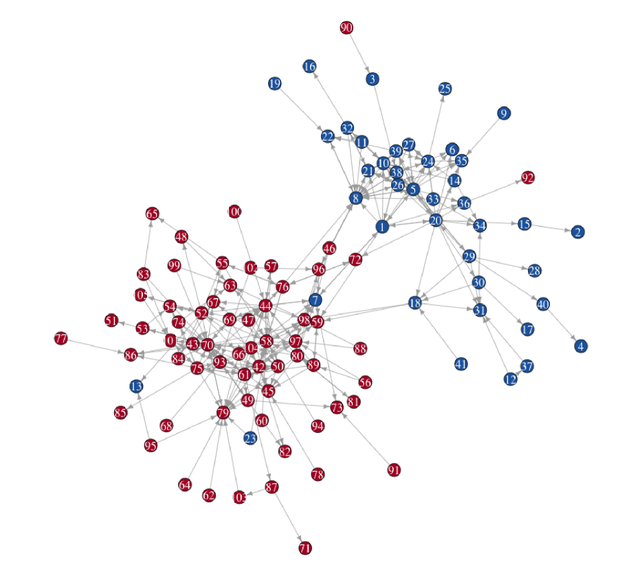
Figure 1: Network Example: True Clustering

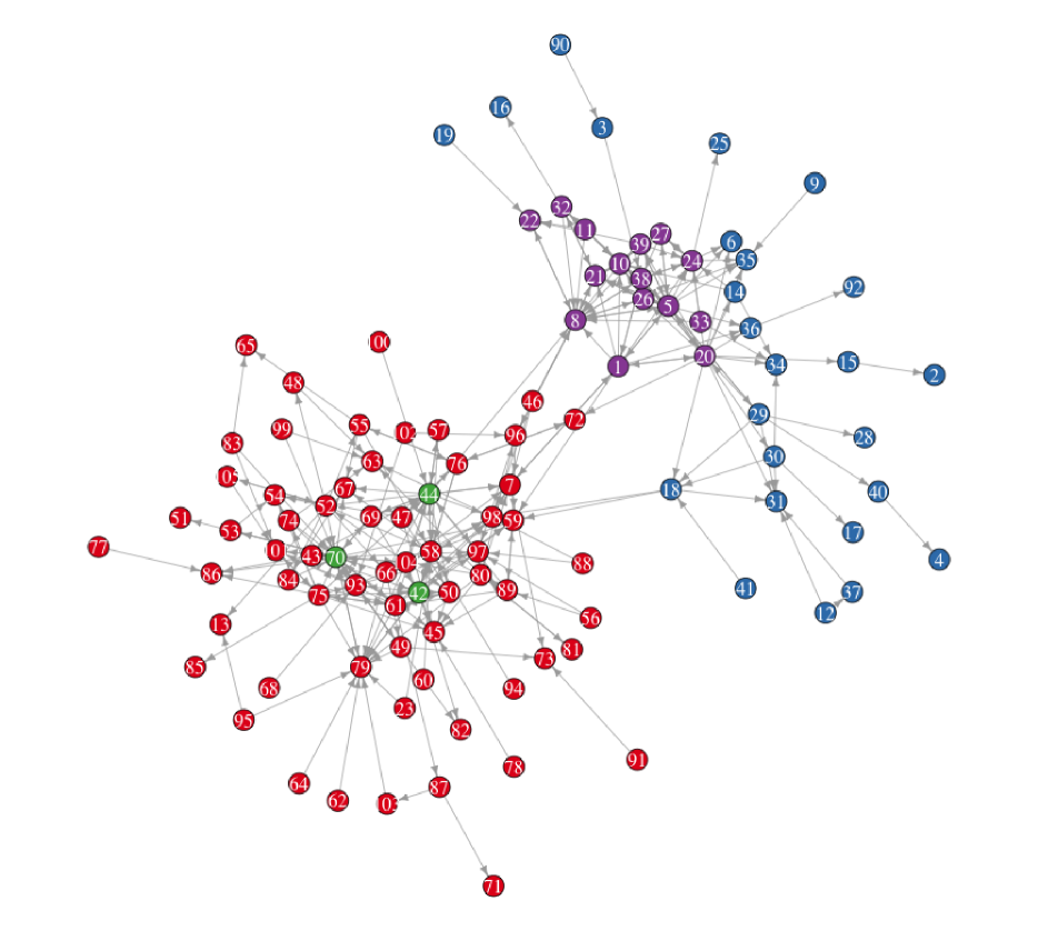
Figure 2: Network Example: Recovered Clustering

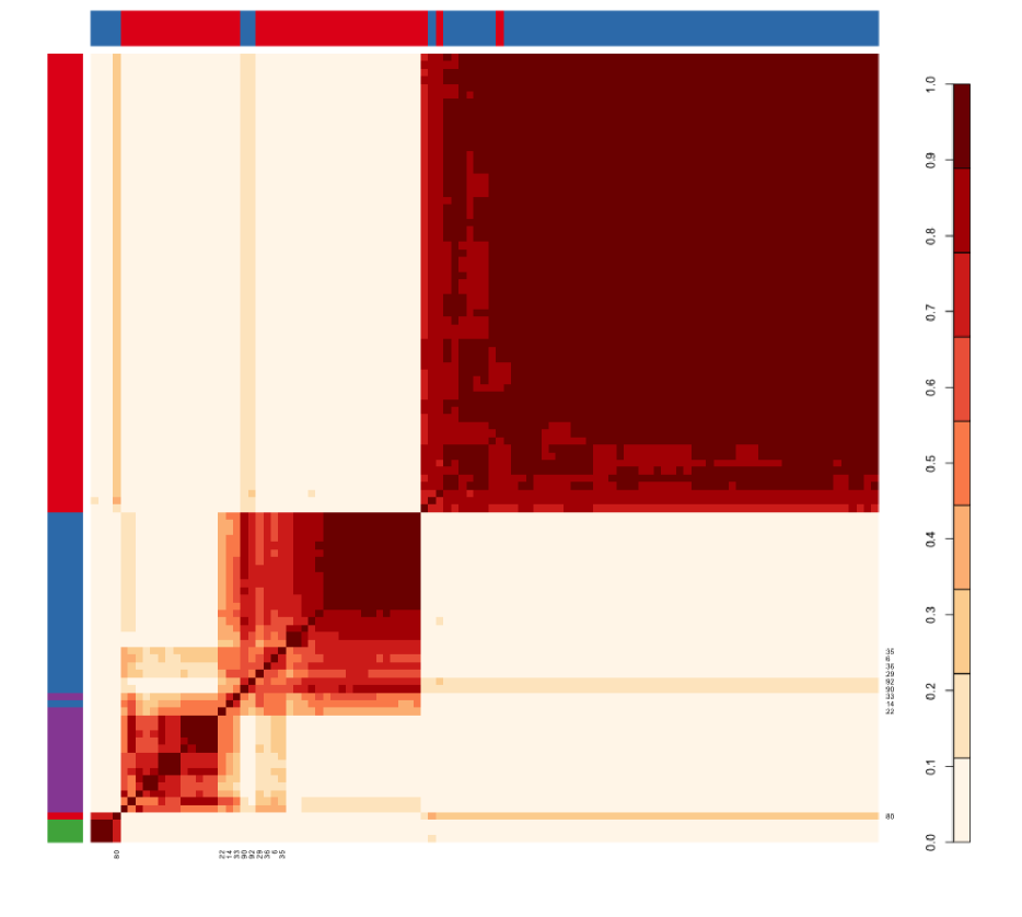
Figure 3: Network Example: Pairwise cluster assignment probability. Left bars correspond to clustering in Fig. 2, top bars correspond to clustering on the ideology label.

Table 3: OAI Data example: Relative Predictive Accuracy. The variables are respectively, left knee baseline pain, isometric strength left knee extension,left knee paired X ray reading, left knee baseline radiographic OA.

	ITF	DPM
P01BL12SXL	31.21	100.92
V00LEXWHY1	7.94	7.56 $\%$
V00XRCHML	23.01	31.84 $\%$
P01LXRKOA	65.78	90.30 $\%$

Acknowledgements

This work was support by Award Number R01ES017436 from the National Institute of Environmental Health Sciences and DARPA MSEE. The content is solely the responsibility of the authors and does not necessarily represent the official views of the National Institute of Environmental Health Sciences or the National Institutes of Health or DARPA MSEE.

References

- Adamic & Glance (2005) Adamic, L. & Glance, N. (2005). The political blogosphere and the 2004 us election: divided they blog. In Proceedings of the 3rd international workshop on Link discovery. ACM.
- Antoniak (1974) Antoniak, C. (1974). Mixtures of dirichlet processes with applications to bayesian nonparametric problems. The annals of statistics , 1152–1174.
- Bigelow & Dunson (2009) Bigelow, J. & Dunson, D. (2009). Bayesian semiparametric joint models for functional predictors. Journal of the American Statistical Association 104, 26–36.
- Cai et al. (2011) Cai, J., Song, X., Lam, K. & Ip, E. (2011). A mixture of generalized latent variable models for mixed mode and heterogeneous data. Computational Statistics & Data Analysis 55, 2889–2907.
- Dunson (2000) Dunson, D. (2000). Bayesian latent variable models for clustered mixed outcomes. Journal of the Royal Statistical Society: Series B (Statistical Methodology) 62, 355–366.
- Dunson (2003) Dunson, D. (2003). Dynamic latent trait models for multidimensional longitudinal data. Journal of the American Statistical Association 98, 555–563.
- Dunson (2009) Dunson, D. (2009). Nonparametric bayes local partition models for random effects. Biometrika 96, 249–262.
- Dunson (2010) Dunson, D. (2010). Multivariate kernel partition process mixtures. Statistica Sinica 20, 1395.
- Dunson & Bhattacharya (2010) Dunson, D. & Bhattacharya, A. (2010). Nonparametric bayes regression and classification through mixtures of product kernels. Bayesian Stats .
- Dunson & Xing (2009) Dunson, D. & Xing, C. (2009). Nonparametric bayes modeling of multivariate categorical data. Journal of the American Statistical Association 104, 1042–1051.
- Escobar & West (1995) Escobar, M. & West, M. (1995). Bayesian density estimation and inference using mixtures. Journal of the american statistical association , 577–588.
- Ferguson (1973) Ferguson, T. (1973). A bayesian analysis of some nonparametric problems. The annals of statistics , 209–230.
- Hannah et al. (2011) Hannah, L. A., Blei, D. M. & Powell, W. B. (2011). Dirichlet process mixtures of generalized linear models. The Journal of Machine Learning Research 12, 1923–1953.
- Li et al. (2011) Li, L., Zhou, M., Wang, E. & Carin, L. (2011). Joint dictionary learning and topic modeling for image clustering. In Acoustics, Speech and Signal Processing (ICASSP), 2011 IEEE International Conference on. IEEE.
- Muthen (1984) Muthen, B. (1984). A general structural equation model with dichotomous, ordered categorical, and continuous latent variable indicators. Psychometrika 49, 115–132.
- Papaspiliopoulos & Roberts (2008) Papaspiliopoulos, O. & Roberts, G. (2008). Retrospective markov chain monte carlo methods for dirichlet process hierarchical models. Biometrika 95, 169–186.
- Sammel et al. (1997) Sammel, M., Ryan, L. & Legler, J. (1997). Latent variable models for mixed discrete and continuous outcomes. Journal of the Royal Statistical Society: Series B (Statistical Methodology) 59, 667–678.
- Sethuraman (1994) Sethuraman, J. (1994). A constructive definition of Dirichlet priors. Statistica Sinica 4, 639–650.
- Shahbaba & Neal (2009) Shahbaba, B. & Neal, R. (2009). Nonlinear models using dirichlet process mixtures. The Journal of Machine Learning Research 10, 1829–1850.
- Shen & Ghosal (2011) Shen, W. & Ghosal, S. (2011). Adaptive bayesian multivariate density estimation with dirichlet mixtures. Arxiv preprint arXiv:1109.6406 .
- Song et al. (2009) Song, X., Xia, Y. & Lee, S. (2009). Bayesian semiparametric analysis of structural equation models with mixed continuous and unordered categorical variables. Statistics in medicine 28, 2253–2276.
- Tokdar (2011) Tokdar, S. (2011). Adaptive convergence rates of a dirichlet process mixture of multivariate normals. Arxiv preprint arXiv:1111.4148 .
- Walker (2007) Walker, S. (2007). Sampling the dirichlet mixture model with slices. Communications in Statistics Simulation and Computation® 36, 45–54.
- Yang & Dunson (2010) Yang, M. & Dunson, D. (2010). Bayesian semiparametric structural equation models with latent variables. Psychometrika 75, 675–693.