Onomastics 2.0
The Power of Social Co-Occurrences

Abstract

Onomastics is “the science or study of the origin and forms of proper names of persons or places.” Especially personal names play an important role in daily life, as all over the world future parents are facing the task of finding a suitable given name for their child. This choice is influenced by different factors, such as the social context, language, cultural background and, in particular, personal taste.

With the rise of the Social Web and its applications, users more and more interact digitally and participate in the creation of heterogeneous, distributed, collaborative data collections. These sources of data also reflect current and new naming trends as well as new emerging interrelations among names.

The present work shows, how basic approaches from the field of social network analysis and information retrieval can be applied for discovering relations among names, thus extending Onomastics by data mining techniques. The considered approach starts with building co-occurrence graphs relative to data from the Social Web, respectively for given names and city names. As a main result, correlations between semantically grounded similarities among names (e. g., geographical distance for city names) and structural graph based similarities are observed.

The discovered relations among given names are the foundation of the Nameling , a search engine and academic research platform for given names which attracted more than 30,000 users within four months, underpinning the relevance of the proposed methodology.

1 Introduction

Most future parents face the challenge of finding a suitable given name for their child. Many non-technical influence factors have to be considered, such as cultural background, social environment, personal preference and current trends. Some factors may even be contradictory, e. g., considering the personal preference of both parents. Even if both parents agree on a favorite given name, often the social environment prevents a final decision, if many children in the neighborhood are given the preferred name. Typically, parents end up browsing through endless lists of thousands of given names, although only a small fraction of those names are “relevant”, considering, e. g., the cultural background and personal preference.

From a technical point of view, the scenario described above forms a challenging recommender setting, where for a given social context (e. g., the parents’ given names, hometown, friends), a list of relevant names is requested. With the rise of the so called “social web”, many sources for background information became available, covering social interaction (e. g., facebook ), encyclopedic knowledge (e. g., Wikipedia ) and short personal messages (e. g., Twitter ).

The present work tackles the task of recommending given names based on data from the social web by analyzing relations among names which are derived from word co-occurrences in Wikipedia and Twitter. Different well known basic approaches for determining the similarity of words are applied and evaluated. The obtained results already gave raise to the Nameling, a search engine for given names which attracted more than 30,000 users within less than four months, underpinning the practical relevance of the discovered relations.

The experiments on name relatedness are preceded by an in-depth comparative analysis of the underlying co-occurrences networks, giving insights into the interrelation of networks derived from different language editions of Wikipedia. The proposed methodological approach can also be seen as a general set up for analyzing and evaluating co-occurrence networks of named entities and respective similarity metrics. Exemplarily, all experiments are conducted in parallel on city names.

This work is structured as follows: Section 2 gives an overview on related topics and respective works. Section 3 summarizes relevant basic concepts and notations, Section 4 and 5 describe the underlying co-occurrence networks and their data sources, together with a comparative analysis of the networks. In Section 6, various similarity functions are described and evaluated, Section 7 finally summarizes the obtained results and points towards future work.

2 Related Work

Early applications of data mining techniques for the analysis of place names include [17], where spatial data of lakes in Finland is analyzed. The application of personal names for estimating ethnicity for census data using data mining is presented in [23]. The task of identifying different variants of named entities is extensively studied, examples include [1, 12, 28, 13, 9, 26]

The present work aims at discovering and assessing new emergent relations among given names based on data from the social web. Methodologically, the considered approach is closely related to work on distributional similarity where, more generally, semantic relations among named entities are investigated. However, this work presents an approach to the discovery and analysis of relatedness from a social network analyst’s point of view, which is connected to the field of link prediction and (more generally) vertex similarity in graphs. The proposed methodology is complementary applied for analyzing the relatedness of city names which relates to work published on Geographic Information Retrieval [27].

Distributional Similarity & Semantic Relatedness:

The field of distributional similarity and semantic relatedness has attracted a lot of attention in literature during the past decades (see [5] for a review). Several statistical measures for assessing the similarity of words are proposed, as for example in [18, 8, 10, 15, 30]. Notably, first approaches for using Wikipedia as a source for discovering relatedness of concepts can be found in [2, 29, 7].

Vertex Similarity & Link Prediction:

In the context of social networks, the task of predicting (future) links is especially relevant for online social networks, where social interaction is significantly stimulated by suggesting people as contacts which the user might know. From a methodological point of view, most approaches build on different similarity metrics on pairs of nodes within weighted or unweighted graphs [11, 16, 20, 21]. A good comparative evaluation of different similarity metrics is presented in [19].

The present work combines approaches from both the link prediction and semantic relatedness tasks with a focus on the structural analysis of the underlying co-occurrence networks and their inter network correlations. Relatedness is considered only for a single class of entities, respectively given names and city names and the obtained results are evaluated in a novel experimental setup which gives also insights into the underlying network structure.

3 Preliminaries

In this chapter, we want to familiarize the reader with the basic concepts and notations used throughout this paper.

A graph $G=(V,E)$ is an ordered pair, consisting of a finite set $V$ of vertices or nodes, and a set $E$ of edges, which are two-element subsets of $V$. A directed graph is defined accordingly: $E$ denotes a subset of $V\times V$. For simplicity, we write $(u,v)\in E$ in both cases for an edge belonging to $E$ and freely use the term network as a synonym for a graph. In a weighted Graph each edge $l\in E$ is given an edge weight $w(l)$ by some weighting function $w\colon E\rightarrow\mathbb{R}$. For a subset $U\subseteq V$ we write ${G}_{|U}$ to denote the sub graph induced by $U$. The density of a graph denotes the fraction of realized links, i. e., $\frac{2m}{n(n-1)}$ for undirected graphs and $\frac{m}{n(n-1)}$ for directed graphs (excluding self loops). The neighborhood $\Gamma$ of a node $u\in V$ is the set of adjacent nodes $\{v\in V\mid(u,v)\in E\}$. The degree of a node in a network measures the number of connections it has to other nodes. For the adjacency matrix $A\in\mathbb{R}^{n\times n}$ with $n=|V|$ holds $A_{ij}=1$ ($A_{ij}=w(i,j)$) iff $(i,j)\in E$ for any nodes $i,j$ in $V$ (assuming some bijective mapping from ${1,\ldots,n}$ to $V$). We represent a graph by its according adjacency matrix where appropriate.

A path $v_{0}\rightarrow_{G}v_{n}$ of length $n$ in a graph $G$ is a sequence $v_{0},\ldots,v_{n}$ of nodes with $n\geq 1$ and $(v_{i},v_{i+1})\in E$ for $i=0,\ldots,n-1$. A shortest path between nodes $u$ and $v$ is a path $u\rightarrow_{G}v$ of minimal length. The transitive closure of a graph $G=(V,E)$ is given by $G^{*}=(V,E^{*})$ with $(u,v)\in E^{*}$ iff there exists a path $u\rightarrow_{G}v$. A strongly connected component (scc) of $G$ is a subset $U\subseteq V$, such that $u\rightarrow_{G^{*}}v$ exists for every $u,v\in U$. A (weakly) connected component (wcc) is defined accordingly, ignoring the direction of edges $(u,v)\in E$.

Many observations of network properties can be explained just by the network’s degree distribution [14]. It is therefore important to contrast the observed property to the according result obtained on a random graph as a null model which shares the same degree distribution. If a single network $G$ is considered, a corresponding null model $\overline{G}$ can be obtained by randomly replacing edges $(u_{1},v_{1}),(u_{2},v_{2})\in E$ with $(u_{1},v_{2})$ and $(u_{2},v_{1})$, ensuring that these edges were not present in $G$ beforehand. This process is typically repeated a multiple of the graph edge set’s cardinality (see [22] for details). For contrasting comparative observations within pairs of networks $(G_{1},G_{2})$, a null model $\underline{G}_{2}$ can be obtained by permuting the vertex positions within $G_{2}$ as described in [4].

4 Data Sources

Wikipedia & Wiktionary

For our analysis we used the official Wikipedia data dump which is freely available for download and considered the English (date: 2012-01-05), French (2012-01-17) and German (2011-12-12) version separately. We additionally used the categorization links of the affiliated Wiktionary project (English, French and German 2012-06-06), also available for download.

Twitter

As an additional source for user generated data we considered the microblogging service Twitter. Using Twitter, each user publishes short text messages (called “tweets”). We used the data set introduced in [31] which comprises 476,553,560 tweets from 17,069,982 users, collected 2009/06 until 2009/12

Given Names

Some effort was made to build up a comprehensive list of given names. In a semi-automatic way, a list of more than 30,000 names was collected. During the first months of the Nameling’s live time, additional names were proposed by users of the system, yielding a list of 36,434 given names.

Cities

As an example for entities with an obvious ad hoc notion of relatedness (namely the geographical distance), we considered cities with a population above 1,000. A corresponding data set which also comprises corresponding geolocations is freely available for download. We eliminated all cities with ambiguous names, resulting in a list of 101,667 city names.

5 Co-occurrence Networks

The present work’s initial motivation was to find relations among given names based on user-generated content in the social web. The most basic relation among such entities can be observed when they occur together within a given atomic context. In case of Wikipedia, we counted such co-occurrences based on sentences and for Twitter based on tweets. We thus obtain for each considered entity type $I\in\{N,C\}$ (given names and city names, respectively) and data source $S\in\{\text{EN},\text{DE},\text{FR},\text{Twitter}\}$ (English, German and French Wikipedia as well as Twitter) an undirected weighted graph $G^{I}_{S}=(V^{I}_{S},E^{I}_{S})$ where $V^{I}_{S}$ denotes the subset of all observed entities of type $I$ within $S$ and for entities $u,v$ exists an edge $(u,v)\in E^{I}_{S}$ with weight $c$, if $u$ and $v$ co-occurred in exactly $c$ contexts.

For example, the given names “Peter” and “Paul” co-occurred in 30,565 sentences within the English Wikipedia whereas the city names “Kassel” and “Göttingen” co-occurred in 630 sentences within the German Wikipedia. Accordingly, there is an edge $(\text{Peter},\text{Paul})$ in $G^{N}_{\text{{EN}}}$ and an edge $(\text{Kassel},\text{G\"{o}ttingen})$ in $G^{C}_{\text{{DE}}}$ respectively with corresponding edge weights.

5.1 High Level Statistics

Table 1 summarizes the high level statistics for all considered co-occurrence networks. As one would expect, all networks contain a giant connected component [25] which almost cover the whole corresponding node sets. The networks obtained from the English Wikipedia are the most densely connected network for given names whereas the French Wikipedia yields the most densely connected network for city names. Networks obtained from Twitter are least densely connected.

Table 1: High level statistics for all Co-occurrence networks.

	$|V|$	$|E|$	density	#wcc	largest wcc
$G^{N}_{\text{{EN}}}$	$27,121$	$24,461,988$	$0.067$	$2$	$27,119$
$G^{N}_{\text{{DE}}}$	$25,032$	$13,172,603$	$0.042$	$2$	$25,030$
$G^{N}_{\text{{FR}}}$	$25,237$	$17,446,139$	$0.055$	$1$	$25,237$
$G^{N}_{\text{Twitter}}$	$25,902$	$6,634,551$	$0.020$	$1$	$25,902$
$G^{C}_{\text{{EN}}}$	$66,060$	$31,015,531$	$0.014$	$22$	$66,014$
$G^{C}_{\text{{DE}}}$	$58,422$	$15,583,628$	$0.009$	$30$	$58,335$
$G^{C}_{\text{{FR}}}$	$55,981$	$30,786,844$	$0.020$	$26$	$55,927$
$G^{C}_{\text{Twitter}}$	$42,512$	$2,651,510$	$0.003$	$46$	$42,419$

5.2 Inter-Network Analysis

Considering the co-occurrence networks presented above, the question whether and to which extent these networks are related naturally arises.

As a first indicator, we considered basic vertex centrality metrics, namely degree centrality and eigenvector centrality as well as the “popularity” of an entity, that is, its global frequency within the corresponding corpus. Please note that we can directly compare centrality scores for nodes within a family of networks (given names and city names respectively), as the vertex sets of these networks are drawn from the same population.

Figure 1 exemplarily shows a pairwise comparison of the degree centrality within different networks $G_{1},G_{2}$. To reduce noise, we calculated for all names having a degree of $k$ in $G_{1}$ the average node degree in $G_{2}$ and scaled the point size logarithmically with the number of corresponding observations. The top left plot, e. g., shows that in average a given name with a degree of 50 in the English Wikipedia has a degree of comparable magnitude in the German Wikipedia. Due to the underlying heavy tailed distributions we plotted in a logarithmic scale. To rule out effects induced by the graphs’ degree distributions, we considered for each pair $G,G^{\prime}$ of networks a corresponding null model $\underline{G}^{\prime}$ (see Sec. 3) where effectively the degree distribution of $G^{\prime}$ is fixed but the vertices are permuted randomly. The results for the null models are averaged for repeated calculations and depicted in gray.

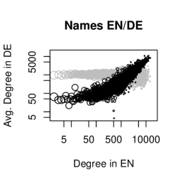
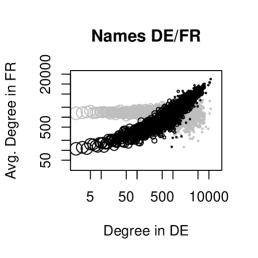
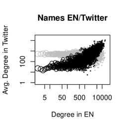
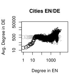
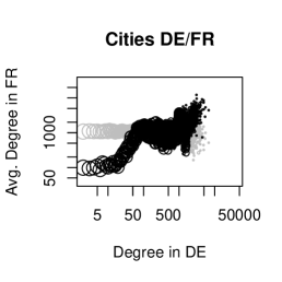
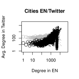
Figure 1: Degree centrality in co-occurrence networks derived from the English (EN), French (FR) and German (DE) Wikipedia, where results obtained from corresponding null models are depicted in gray.

As a general trend, positive correlations for the degree centrality can be observed in all networks for given names, though less pronounced for the Twitter based network and for lower vertex degrees but significantly deviating from correlations obtained from a corresponding null model.

For the city name networks, positively correlated trends can only be observed for lower degree nodes in the Wikipedia based networks. For the Twitter based network the result is comparable with the given names networks. Please note the significant cluster of nodes with high degree centrality in the English Wikipedia and low centrality scores for the other networks. Manual inspection showed that these are indeed results of corresponding distinct city names and not names with common words. These outliers can not be explained just by analyzing the network structure and therefor the word contexts within the corpora must be considered which is out of the present work’s scope.

In contrast to the degree centrality, the eigenvector centrality appears to reveal distinct trends for given names within the corresponding co-occurrence networks. Figure 2 exemplarily shows the comparative plots for eigenvector centrality within pairs of given name networks. In both cases, the lower right area is (by trend) populated with classic German names whereas the upper left area is populated by English and French names, respectively. These language specific characteristics of the eigenvector centrality can be exploited for automatically classifying given names according to their cultural background.

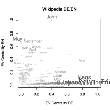
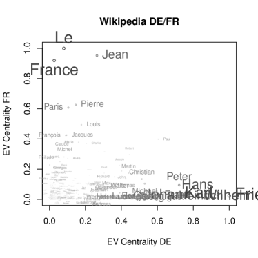
Figure 2: Pairwise comparison of eigenvector centrality for co-occurrence networks of given names based on Wikipedia in English, French and German.

For the city names networks, the eigenvector centrality exhibits only very sparse distinct language specific trends which are dominated by city names which coincide with common words of the respective language, as for example “England”, “Collage” and “Church” for English and “Das”, “Die”, “Band” for German. Most of the centrality scores are clustered together and show a significantly correlated trend in the corresponding log-scale plot in Fig. 3. For visualizing the geographical reference of the denoted cities, we colored each point according to the respective geographic location, where latitude and longitude are used to select a color within the HSL color space (see the top right earth globe projection in Fig. 3). Please note that points are plotted ordered according to the corresponding longitude value for unifying the effect of covered areas. Comparing with the null model (obtained by comparing $G^{C}_{\text{DE}}$ with $\underline{G}^{C}_{\text{EN}}$), Fig. 3 reveals a correlated trend for the eigenvector centrality of city names in the different language specific editions of Wikipedia and points towards an interrelation of the geographic location of a city and its position within the co-occurrence networks. We will investigate this interrelation more detailed in Sec. 6.1.

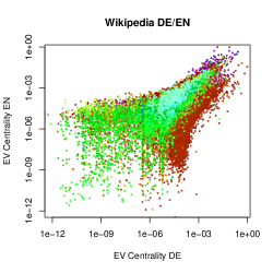
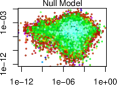
Figure 3: Pairwise comparison of eigenvector centrality for co-occurrence networks of city names based on Wikipedia in English and German.

5.3 Inter-Network Correlation Test

For a more formalized analysis, we assess the network interrelation in terms of the correlation of the corresponding adjacency matrices by applying the quadradic assignment procedure (QAP) test [3, 4].

For given graphs $G_{1}=(V_{1},E_{1})$ and $G_{2}=(V_{2},E_{2})$ with $U\mathrel{\mathop{:}}=V_{1}\cap V_{2}\neq\emptyset$ and adjacency matrices $A_{i}$ corresponding to ${G_{i}}_{|U}$ ($G_{i}$ reduced to the common vertex set $U$, see Sec. 3), the graph covariance is given by

$$\mathop{cov}(G_{1},G_{2})\mathrel{\mathop{:}}=\frac{1}{n^{2}-1}\sum_{i=1}^{n}\sum_{j=1}^{n}(A_{1}[i,j]-\mu_{1})(A_{2}[i,j]-\mu_{2})$$

where $n\mathrel{\mathop{:}}=|U|$ and $\mu_{i}$ denotes $A_{i}$’s mean ($i=1,2$). Then $\mathop{var}(G_{i})\mathrel{\mathop{:}}=\mathop{cov}(G_{i},G_{i})$ leading to the graph correlation

$$\rho(G_{1},G_{2})\mathrel{\mathop{:}}=\frac{\mathop{cov}(G_{1},G_{2})}{\sqrt{\mathop{var}(G_{1})\mathop{var}(G_{2})}}.$$

The QAP test compares the observed graph correlation $\rho_{0}$ to the distribution of resulting correlation scores obtained on repeated random row/column permutations of $A_{2}$. The fraction of permutations $\pi$ with correlation $\rho^{\pi}\geq\rho_{o}$ is used for assessing the significance of an observed correlation score $\rho_{o}$. Intuitively, the test determines (asymptotically) the fraction of all graphs with the same structure as $G_{2|U}$ having at least the same level of correlation with $G_{1|U}$.

Table 2 shows the pairwise correlation scores for all considered networks. Consistent with our preceding observations, the Wikipedia-based co-occurrence shows the strongest correlations, significantly more pronounced for given names. For assessing the significance of the observed correlations, we repeatedly calculated the pairwise correlations on 1,000 corresponding randomly generated null models. For any pair of the considered networks, every randomly generated null model showed much lower correlation scores ($<10^{-3}$), which indicates according to [3] statistical significance.

We conclude that the co-occurrence networks structurally correlate, more pronounced though for given names than for city names. Nevertheless, language specific deviations exist. For discovering relations on named entities the corresponding language should therefore be considered. In the next section we will investigate, how relations can be extracted from the co-occurrence networks and how these relations correlate with natural notions of relatedness.

Table 2: Pairwise graph correlation observed in the co-occurrence graphs.

	$G^{N}_{\text{{EN}}}$	$G^{N}_{\text{{DE}}}$	$G^{N}_{\text{{FR}}}$	$G^{N}_{\text{Twitter}}$
$G^{N}_{\text{{EN}}}$	-	$0.406$	$0.332$	$0.049$
$G^{N}_{\text{{DE}}}$	-	-	$0.303$	$0.020$
$G^{N}_{\text{{FR}}}$	-	-	-	$0.015$
$G^{N}_{\text{Twitter}}$	-	-	-	-

	$G^{C}_{\text{{EN}}}$	$G^{C}_{\text{{DE}}}$	$G^{C}_{\text{{FR}}}$	$G^{C}_{\text{Twitter}}$
$G^{C}_{\text{{EN}}}$	-	$0.119$	$0.180$	$0.067$
$G^{C}_{\text{{DE}}}$	-	-	$0.135$	$0.025$
$G^{C}_{\text{{FR}}}$	-	-	-	$0.040$
$G^{C}_{\text{Twitter}}$	-	-	-	-

6 Mining for Relations from the Social Web

In the previous section, two kinds of co-occurrence networks were introduced, one for given names and the other for city names. These networks were structurally analyzed and compared, giving insights into immanent properties and correlations among different networks. Keeping in mind the initial motivation for the present work, namely the recommendation of given names based on data from the social web, we now focus on the question, whether the co-occurrence networks from Section 5 give raise to a notion of relatedness which implies relationships the user might be interested in.

For evaluating different similarity metrics based on the co-occurrence networks, we need a “reference” notion of relatedness for the considered entities to be used as “ground truth”. For cities, the geographic distance is a natural candidate. For given names, such generally accepted reference relation is less obvious. We therefor apply the approach of using an external data source which we assume as a valid “gold standard”. We argue that the categories assigned to names in Wiktionary are a good basis, as they are manually assigned and have a direct connection to concepts users associate with given names (such as gender and cultural context). We finally chose cosine similarity (see Sec. 6.1) for calculating a reference similarity score, which is broadly accepted for various applications. For simplicity we restrict our analysis in this chapter to the English Wikipedia.

In the following, we will first introduce different similarity functions for calculating similarity of named entities based on corresponding co-occurrence networks. We will than compare these similarity functions for given names and city names, respectively, with the corresponding gold standard relations described above.

6.1 Vertex Similarities

Similarity scores for pairs of vertices based only on the surrounding network structure have a broad range of applications, especially for the link prediction task [19]. In the following we present all considered similarity functions, following the presentation given in [6] which builds on the extensions of standard similarity functions for weighted networks from [24]. The Jaccard coefficient measures the fraction of common neighbors:

$$\mathop{JC}(x,y)\mathrel{\mathop{:}}=\frac{|\Gamma(x)\cap\Gamma(y)|}{|\Gamma(x)\cup\Gamma(y)|}$$

The Jaccard coefficient is broadly applicable and commonly used for various data mining tasks. For weighted networks the Jaccard coefficient becomes:

$$\widetilde{\mathop{JC}}(x,y)\mathrel{\mathop{:}}=\sum_{z\in\Gamma(x)\cap\Gamma(y)}\frac{w(x,z)+w(y,z)}{\sum_{a\in\Gamma(x)}w(a,x)+\sum_{b\in\Gamma(y)}w(b,y)}$$

The resource allocation index $\mathop{R\!A}$ [32] captures the intuition that for two nodes $x$ and $y$, the importance of a common neighbor $z$ to their relatedness depends on how “exclusive” $z$ connects $x$ with $y$:

$$\mathop{R\!A}(x,y)\mathrel{\mathop{:}}=\sum_{z\in\Gamma(x)\cap\Gamma(y)}\frac{1}{|\Gamma(z)|}$$

The $\mathop{R\!A}$ for weighted networks is given by

$$\widetilde{\mathop{R\!A}}(x,y)\mathrel{\mathop{:}}=\sum_{z\in\Gamma(x)\cap\Gamma(y)}\frac{w(x,z)+w(y,z)}{\sum_{c\in\Gamma(z)}w(z,c)}.$$

Similar to $\mathop{R\!A}$, the Adamic-Adar coefficient captures the exclusiveness of common neighbors, though respecting underlying power distributions:

$$\mathop{A\!A}(x,y)\mathrel{\mathop{:}}=\sum_{z\in\Gamma(x)\cap\Gamma(y)}\frac{1}{\log(|\Gamma(z)|)}$$

For weighted networks, the Adamic-Adar coefficient is defined as

$$\widetilde{\mathop{A\!A}}(x,y)\mathrel{\mathop{:}}=\sum_{z\in\Gamma(x)\cap\Gamma(y)}\frac{w(x,z)+w(y,z)}{\log(1+\sum_{c\in\Gamma(z)}w(z,c))}.$$

The cosine similarity measures the cosine of the angle between the corresponding rows of the adjacency matrix, which for a unweighted graph can be expressed as

$$\mathop{C\!O\!S}(x,y)\mathrel{\mathop{:}}=\frac{|\Gamma(x)\cap\Gamma(y)|}{\sqrt{|\Gamma(x)|}\cdot\sqrt{|\Gamma(y)|}},$$

and for a weighted graph is given by

$$\widetilde{\mathop{C\!O\!S}}(x,y)\mathrel{\mathop{:}}=\sum_{z\in\Gamma(x)\cap\Gamma(y)}\frac{w(x,z)w(y,z)}{\sqrt{\sum_{a\in\Gamma(x)}w(x,a)^{2}}\cdot\sqrt{\sum_{b\in\Gamma(y)}w(y,b)^{2}}}.$$

The vertex similarity introduced in [16] measures the observed number of common neighbors relative to the overlap expected in a corresponding random graph:

$$\mathop{N\!EW}(x,y)\mathrel{\mathop{:}}=\frac{|\Gamma(x)\cap\Gamma(y)|}{|\Gamma(x)||\Gamma(y)|}$$

6.2 Given Names

For obtaining a reference relation on the set of given names, we collected all corresponding category assignments from Wiktionary. We thus obtained for each of 10,938 given names a respective binary vector, where each component indicates whether the corresponding category was assigned to it (in total 7,923 different categories and 80,726 non-zero entries). As these assignment vectors are very sparse, we counted for each name the number of name pairs with a non-zero similarity score, to ensure that a relevant similarity metric is induced. Indeed, more than 90% of the names had more than one hundred “similar” names.

For any pair $u,v$ of names in the co-occurrence network which have a category assignment, we calculated the cosine similarity $\mathop{C\!O\!S}(u,v)$ based on the respective category assignment vectors as well as any of the similarity metrics $s(u,v)$ described in section 6.1. As the number of data points $(\mathop{C\!O\!S}(uv),S(u,v))$ grows quadratically with the number of names, we grouped the co-occurrence based similarity scores in 1,000 equidistant bins and calculated for each bin the average cosine similarity based on category assignments. Figure 4 shows the results for Wikipedia and Twitter separately.

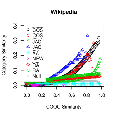
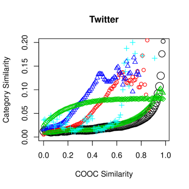
Figure 4: Similarity based on name categories in Wiktionary vs. vertex similarity in the co-occurrence-networks (weighted and unweighted).

Notably all but Adamic-Adar and $\mathop{N\!EW}$ capture a positive correlation between similarity in the co-occurrence network and similarity between category assignments to names. But significant differences between the underlying co-occurrence networks and the applied similarity functions can be observed. As for Wikipedia, the weighted cosine similarity performs very well, firstly in showing a steep slope and secondly in exhibiting a stable monotonous curve progression. The unweighted Jaccard coefficient also shows an even more pronounced linear progression, but is less stable for higher similarity scores whereas the weighted Jaccard coefficient shows a higher correlation with the reference similarity for high similarity scores.

As for Twitter, no globally best matching similarity score can be found. Each of the similarity functions shows good progression only in parts. Considering only cosine similarity and the Jaccard coefficient, we see that both in the unweighted case show higher correlations with the semantic similarity for mid range similarity scores, whereas in the weighted case, both exhibit higher correlations for higher similarity scores.

6.3 City Names

We conducted the same experiment as in section 6.2 for city names, using the geographical distance of corresponding pairs of cities as a reference relation. As we only considered cities with a unique name in the data set (see Sec. 4) and each city has a distinct geographical location associated, we thus obtained a dense reference relation with explicit real world semantics associated.

We calculated for each pair $u,v$ of city names the geographical distance $d(u,v)$ and similarity $s(u,v)$ in the co-occurrence networks (see Sec. 6.1). As the number of data points grows quadratically with the number of city names, we grouped the co-occurrence based similarity scores in 1,000 equidistant bins and calculated for each bin the average geographical distance. Figure 5 shows the resulting plots for all considered similarity functions on the Wikipedia and Twitter-based co-occurrence networks separately.

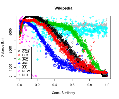
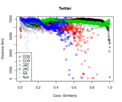
Figure 5: Geographic distance between cities versus vertex similarites in the co-occurrence-networks (weighted and unweighted).

Considering the results obtained on Wikipedia, cosine similarity and the Jaccard coefficient show a strikingly high correlation with the geographical distance. For the cosine similarity and the weighted Jaccard coefficient, a negative correlation can be observed for similarity scores $\leq 0.2$ which is also present for the unweighted Jaccard coefficient for low similarity scores $\leq 0.05$. We also counted the number of observations per bin to rule out effects induced by averaging the geographical distance, but no significant accumulation of low similarity scores $\leq 0.2$ could be observed. We conclude that low similarity scores in the co-occurrence based networks are less significant. Both cosine similarity and Jaccard coefficient show more stable results in the weighted variant, where cosine similarity shows most significant correlations for mid-range similarity scores whereas the Jaccard coefficient performs best for higher similarity scores. For all other similarity metrics, no correlation can be observed, where the resource allocation index is excluded for a clearer presentation.

As for Twitter, no significant correlation between structural similarity in the co-occurrence network and geographical distance can be observed, despite a very small range around very high similarity scores of the weighted cosine similarity. The next section investigates this deviating characteristics in more details.

6.4 Neighborhood & Similarity

In the preceding sections, the correlation of external reference measures of semantic relatedness with different similarity functions in the co-occurrence networks was analyzed. For given names, correlations could be observed in networks obtained from Wikipedia and Twitter, whereas for city names, the Wikipedia based analysis showed astonishing high correlations in contrast to the Twitter based network, where no significant correlations could be observed.

For further analysis, we considered a very basic measure of relatedness between two nodes in a network, namely their respective shortest path distance. We asked, whether names which are direct neighbors in the co-occurrence graph tend to be more similar than distant names and whether cities which occur together tend to be located geographically nearby. That is, for every shortest path distance $d$ and every pair of nodes $u,v$ with a shortest path distance $d$, we calculated the average corresponding similarity score ($\mathop{C\!O\!S}(u,v)$ and $\mathop{JC}(u,v)$ for given names and geographic distance between $u$ and $v$ for city names). To rule out statistical effects, we repeated for each network $G$ the same calculations on corresponding null model graphs $\underline{G}$.

Figure 6 shows the results for given names and the cosine similarity together with the Jaccard coefficient as well as for city names and geographical distance. For given names, in both networks the similarity of node pairs tends to decrease monotonically with the respective shortest path distance, where direct neighbors are in average more similar than randomly chosen pairs (refer to the null model baseline) and pairs at distance two are already less similar than expected by chance. As for city names, the Wikipedia based network shows an positive correlation of shortest path distance with geographical distance, where the deviating behavior of nodes at distance six is not statistically significant, as only 83 pairs of nodes with corresponding distance exist (in contrast to over 31 million direct neighbors). Most notably, the relationship of geographical distance and shortest path distance in the Twitter based network is inverse. Further experimentation for explaining this deviating semantics are out of the scope of the present work. But it shows that the semantics induced by co-occurrence in Twitter differs from the semantics induced by Wikipedia. It explains the difference in the observed correlations for similarity and geographical distance of city names in Wikipedia and Twitter based co-occurrence networks in Sec. 6.3, as the considered similarity functions only depend on the direct neighborhood.

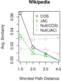
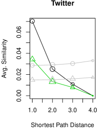
(a)

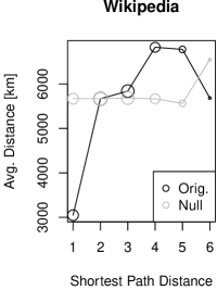
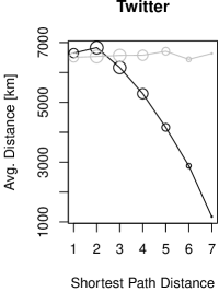
(b)

Figure 6: Semantic relatedness vs. shortest path distance in the co-occurrence networks.

7 Conclusion & Future Work

With the present work, we introduce the task of discovering relatedness of given names based on data from the social web. Our experiments, on the one side, show promising results already for well known basic approaches, namely co-occurrence based similarity calculations. On the other side, the presented analysis builds an experimental framework for analyzing semantics captured by different co-occurrence networks. The present work already yields results of practical relevance, underpinned by the success of the Nameling, which allows users to browse through given names, using the discovered relations among given names derived from co-occurrence networks in Wikipedia.

In Section 5.2, co-occurrence networks derived from Wikipedia in different languages are compared. The eigenvector centrality based comparative analysis revealed language specific features, both for given names and city names. This result suggests that features derived from co-occurrence networks of different languages of Wikipedia can be used to train classifiers for detecting language specific entities. We plan to implement and evaluate such classifiers for labeling given names according to their language association and incorporate the obtained results in the Nameling.

Section 6 focused on the evaluation of different similarity metrics, relative to a respectively fixed notion of semantic relatedness. Firstly, the considered list of similarity functions is not exhaustive. Especially, all considered similarity functions only considered local features, i. e., based on the direct neighborhood. Accordingly, we will evaluate more similarity functions. But also for the reference relation more alternatives have to be considered. From a practical point of view, different types of relatedness among given names are of interest, as, e. g., language specific variants or originating cultural background. Different similarity functions may capture different forms of semantic relatedness. Furthermore, the experimental set up in Section 6 can be used to formulate a machine learning task, aiming at optimizing a similarity function based on features derived from the co-occurrence networks.

We will apply the Nameling’s usage statistics for evaluating different similarity functions with respect to human interaction in a specific recommender scenario.

References

- [1] D. Bikel, R. Schwartz, and R. Weischedel. An algorithm that learns what’s in a name. Machine Learning, 34(1-3):211–231, 1999.
- [2] R. Bunescu and M. Pasca. Using encyclopedic knowledge for named entity disambiguation. In Proc. of EACL, volume 6, pages 9–16, 2006.
- [3] C. Butts. Social network analysis: A methodological introduction. Asian J. of Soc. Psychology, 11(1):13–41, 2008.
- [4] C. T. Butts and K. M. Carley. Some simple algorithms for structural comparison. Comput. Math. Organ. Theory, 11:291–305, December 2005.
- [5] T. Cohen and D. Widdows. Empirical distributional semantics: methods and biomedical applications. J Biomed Inform, 42(2):390–405, Apr. 2009.
- [6] H. de Sá and R. Prudencio. Supervised link prediction in weighted networks. In Neural Networks (IJCNN), The 2011 Int. Joint Conference on, pages 2281–2288. IEEE, 2011.
- [7] E. Gabrilovich and S. Markovitch. Computing semantic relatedness using wikipedia-based explicit semantic analysis. In Proc. of the 20th int. joint conference on artificial intelligence, volume 6, page 12. Morgan Kaufmann Publishers Inc., 2007.
- [8] G. Grefenstette. Finding semantic similarity in raw text: The deese antonyms. In Fall Symposium Series, Working Notes, Probabilistic Approaches to Natural Language, pages 61–65, 1992.
- [9] U. Hermjakob, K. Knight, and H. Daumé III. Name translation in statistical machine translation: Learning when to transliterate. Proceedings of ACL-08: HLT, pages 389–397, 2008.
- [10] A. Islam and D. Inkpen. Second order co-occurrence pmi for determining the semantic similarity of words. In Proc. of the Int. Conference on Language Resources and Evaluation (LREC 2006), pages 1033–1038, 2006.
- [11] G. Jeh and J. Widom. Simrank: a measure of structural-context similarity. In Proc. of the eighth ACM SIGKDD int. conference on Knowledge discovery and data mining, KDD ’02, pages 538–543, New York, NY, USA, 2002. ACM.
- [12] L. Jiang, M. Zhou, L.-F. Chien, and C. Niu. Named entity translation with web mining and transliteration. In Proceedings of the 20th international joint conference on Artifical intelligence, pages 1629–1634. Morgan Kaufmann Publishers Inc., 2007.
- [13] V. Jijkoun, M. A. Khalid, M. Marx, and M. de Rijke. Named entity normalization in user generated content. In Proceedings of the second workshop on Analytics for noisy unstructured text data, AND ’08, pages 23–30, New York, NY, USA, 2008. ACM.
- [14] E. Kolaczyk. Statistical analysis of network data: Methods and models. Springer Series In Statistics, page 386, 2009.
- [15] T. Landauer and S. Dumais. A solution to plato’s problem: The latent semantic analysis theory of acquisition, induction, and representation of knowledge. Psychological Review, 104(2):211, 1997.
- [16] E. A. Leicht, P. Holme, and M. E. J. Newman. Vertex similarity in networks, 2005. cite arxiv:physics/0510143.
- [17] A. Leino, H. Mannila, and R. Pitkänen. Rule discovery and probabilistic modeling for onomastic data. Knowledge discovery in databases: PKDD 2003, pages 291–302, 2003.
- [18] M. Lesk. Word-word associations in document retrieval systems. American documentation, 20(1):27–38, 1969.
- [19] D. Liben-Nowell and J. Kleinberg. The link-prediction problem for social networks. J. of the American society for inf. science and technology, 58(7):1019–1031, 2007.
- [20] L. Lü, C. Jin, and T. Zhou. Similarity index based on local paths for link prediction of complex networks. Physical Review E, 80(4):046122, 2009.
- [21] L. Lü and T. Zhou. Link prediction in weighted networks: The role of weak ties. EPL (Europhysics Letters), 89:18001, 2010.
- [22] S. Maslov and K. Sneppen. Specificity and stability in topology of protein networks. Science, 296(5569):910, 2002.
- [23] P. Mateos. An ontology of ethnicity based upon personal names: with implications for neighbourhood profiling. PhD thesis, University College London, 2007.
- [24] T. Murata and S. Moriyasu. Link prediction of social networks based on weighted proximity measures. In Web Intelligence, IEEE/WIC/ACM Int. Conference on, pages 85–88. IEEE, 2007.
- [25] M. E. J. Newman. The structure and function of complex networks. SIAM Review, 45(2):167–256, 2003.
- [26] J. Nothman, N. Ringland, W. Radford, T. Murphy, and J. R. Curran. Learning multilingual named entity recognition from wikipedia. Artificial Intelligence, 194(0):151 – 175, 2013. Artificial Intelligence, Wikipedia and Semi-Structured Resources.
- [27] S. E. Overell and S. Rüger. Geographic co-occurrence as a tool for gir. In Proc. of the 4th ACM workshop on Geographical information retrieval, GIR ’07, pages 71–76, New York, NY, USA, 2007. ACM.
- [28] R. Steinberger and B. Pouliquen. Cross-lingual named entity recognition. Lingvisticae Investigationes, 30(1):135–162, 2007.
- [29] M. Strube and S. P. Ponzetto. Wikirelate! computing semantic relatedness using wikipedia. In proc. of the 21st national conference on Artificial intelligence - Volume 2, AAAI’06, pages 1419–1424. AAAI Press, 2006.
- [30] P. Turney. Mining the web for synonyms: Pmi-ir versus lsa on toefl. In Proc. of the 12th European Conference on Machine Learning, pages 491–502. Springer-Verlag, 2001.
- [31] J. Yang and J. Leskovec. Patterns of temporal variation in online media. In Proc. of the fourth ACM int. conference on Web search and data mining, pages 177–186. ACM, 2011.
- [32] T. Zhou, L. Lü, and Y. Zhang. Predicting missing links via local information. The European Physical J. B-Condensed Matter and Complex Systems, 71(4):623–630, 2009.