Detecting non-Abelian geometric phase in circuit QED

Abstract

We propose a scheme for detecting noncommutative feature of the non-Abelian geometric phase in circuit QED, which involves three transmon qubits capacitively coupled to an one-dimensional transmission line resonator. By controlling the external magnetic flux of the transmon qubits, we can obtain an effective tripod interaction of our circuit QED setup. The noncommutative feature of the non-Abelian geometric phase is manifested that for an initial state undergo two specific loops in different order will result in different final states. Our numerical calculations show that this difference can be unambiguously detected in the proposed system.

Phase factor has played a profound role in quantum physics. Apart from the familiar dynamical phase, geometric phase (GP), discovered in 1984 by Berry Berry , has deep physical meanings. Berry pointed out that GP occurs when a system is subjected to a cyclic adiabatic evolution, which results from the geometrical properties of the parameter space of the Hamiltonian. Especially, Wilczek and Zee found non-Abelian gauge phase results from Berry’s formula in 1984 FZ . GP depends only on the solid angle enclosed by the parameter path, and thus is robust against local noises AIM ; GD ; AIMV ; PPN ; IFE ; SJY ; zhuerror . Therefore, it has been proposed to implement fault-tolerant quantum logical gates for universal quantum computation Zanardi ; Pachos ; Jones ; Duan ; zhuunconventional ; xue .

Non-Abelian GP differs from Abelian geometric phase according to the commutation features of their gauge potential, i.e., an initial state undergoes two specific cyclical evolution in different order will result in different final states. Up to now, Abelian GP has been experimentally detected in various systems Tycko ; e ; f , while non-Abelian GP has not been verified yet. Usually, dark states are used in detecting GP so that dynamical phase will not appear. Conventionally, it is the tripod Hamiltonian that has been proposed to detect the non-Abelian GP RBK ; Zhang ; JGP . However, it is difficult to find tripod configuration atomic energy levels, which impedes experimental detection of the non-Abelian GP. Recently, it is also proposed that non-Abelian GP can be detected by two laser beams interacting with a three-level $\Lambda$ atom in cold atomic system Du ; eric . Since two of the eigenstates in this scheme are only near degenerate, dynamical phases will also occur during the process, and thus one needs additional effort to conceal it Du . Meanwhile, the non-Abelian GP is also proposed to be detected in a new designed multi-level superconducting circuit feng . However, multi-level scenario of this superconducting nanocircuit is very sensitive to its background charge noise. Therefore, to certify the fundamental non-Abelian nature of the non-Abelian GP, it is of great importance to find an experimentally accessible system that can host the exotic non-Abelian structure.

Superconducting system is regarded as one of the most promising candidates for physical implementation of qubits which can support scalable quantum information processing you ; nori . Furthermore, by placing superconducting qubits in a cavity, i.e, circuit QED setup cqed ; ARA , the system will have several practical advantages including strong coupling strength, immunity to noises, and suppression of spontaneous emission. Here, we propose to detect the noncommutative feature of non-Abelian GP with effective tripod Hamiltonian in circuit QED. The setup we consider consists three transmon qubits that are capacitively coupled to an one-dimensional (1D) high-Q transmission line resonator (cavity), which has recently been realized experimentally exp . With proper chosen parameters, such setup can be effectively described by the tripod Hamiltonian tripod , and thus can be used to detect the noncommutative feature of non-Abelian GP. Furthermore, the transmon qubit possesses remarkable superiority JTJ , e.g., it achieves exponential insensitivity to charge noise without increasing the sensitivity to either flux or critical-current noise. Note that when adding a shunt capacitor to a flux qubit will also lead to low-decoherence qubit t2 .

The considered circuit QED architecture is shown in Fig. 1 with three identical transmon qubits that are capacitively coupled to the cavity. The transmon qubit has effective Josephson energy $E_{J}=E_{J,max}|{\cos(\pi\Phi/\Phi_{0})}|$ with $E_{J,max}$, $\Phi$ and $\Phi_{0}$ being the Josephson energy of the Josephson junctions, the external magnetic flux and the flux quantum, respectively. This type of qubit has good coherence performance. The charging energy of the transmon is much small compared with the Josephson energy ($E_{C}{\ll}E_{J}$). With $E_{J}/E_{C}=50$ ($E_{C}=0.3$ GHz, $E_{J}=15$ GHz), the energy difference of the two lowest levels (defined as first excited state $|e\rangle$ and ground state $|g\rangle$) is approximately $\sqrt{8E_{J}E_{C}}$, and the relaxation time for $|e\rangle$ is on the order of 0.06 s JTJ . For an 1D cavity with length $L=\lambda=1$ cm, we can get rms voltage $V^{0}_{rms}=\sqrt{\hbar\omega/lc}$ of an antinode between two superconducting lines, where $l$ and $c$ are the inductance and capacitance per unit length, respectively. As a result, qubits are coupled to the superconducting line by means of the voltage $\hat{V}=V^{0}_{rms}(\hat{a}+\hat{a}^{{\dagger}})$. Remarkably, for coplanar waveguide cavity, cavity quality factor $Q\sim 10^{6}$ has already been demonstrated PHB , which means that the internal losses can be very low. With three qubits fabricated at the antinodes of the cavity voltage, the strength of the coupling to the resonator is maximized for all three transmom qubits. Then, the system can be described by the Tavis-Cummings Hamiltonian

$$\hat{H}_{TC}=\hbar\omega\hat{a}^{{\dagger}}\hat{a}+\sum_{i=1}^{3}{\left[{1\over 2}\hbar\varepsilon_{i}\hat{\sigma}_{z}^{i}+{\hbar}g_{i}(\hat{\sigma}_{+}^{i}\hat{a}+\hat{\sigma}_{-}^{i}\hat{a}^{{\dagger}})\right]},$$ (1)

where $\omega=1/\sqrt{lc}$ is the resonator frequency, $\hat{a}$ ($\hat{a}^{{\dagger}}$) is annihilation (creation) operator of the 1D cavity mode, $\varepsilon_{i}=\sqrt{8E_{c}^{i}E_{J}^{i}}/\hbar$ is the energy splitting of the $i$th qubit, $\hat{\sigma}^{i}$ are Pauli operator for the $i$th transmon, and $g_{i}=2eC_{g}^{i}V^{0}_{rms}(E_{J}^{i}/8E_{{}_{C}}^{i})^{1/4}/{\sqrt{2}C_{{}_{\Sigma}}^{i}}$ is the strength of coupling between the $i$th qubit and the superconducting line. For $C_{g}/C_{{}_{\Sigma}}=0.1$ with $C_{{}_{\sum}}=C_{g}+2C_{J}$, the coupling strength controlled by external magnetic flux $\Phi_{i}$ will be on the order of 100 MHz ARA . Describe $\varepsilon_{i}$ and $g_{i}$ of Hamiltonian in Eq. (1) in external magnetic flux $\Phi_{i}$, they read

$$\hbar\varepsilon_{i}(\Phi_{i})=\sqrt{8E^{i}_{C}E^{i}_{J,max}|\cos(\frac{\pi\Phi_{i}}{\Phi_{0}})|},$$ (2a)

$$g_{i}(\Phi_{i})=\sqrt{2e^{2}}\frac{C_{g}^{i}}{C_{\Sigma}^{i}}V^{0}_{rms}(\frac{E_{J,max}^{i}}{8E_{C}^{i}})^{1/4}|(\cos\frac{\pi\Phi_{i}}{\Phi_{0}})|^{1/4}.$$ (2b)

Explicitly, the coupling strength $g_{i}$ and the qubit frequency $\varepsilon_{i}$ are endowed with a relation $g_{i}(\Phi_{i})\varpropto\sqrt{\varepsilon_{i}(\Phi_{i})}$.

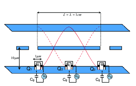
Figure 1: (Color online) Schematic of the circuit QED architecture. The 1D superconducting line resonator consists of a full-wave section ( $L=\lambda=1$cm ) of superconducting coplanar waveguide. Qubits placed between superconducting line resonators consist of two small Josephson junctions, which permit tuning of the effective Josephson energy by an external flux $\Phi$ in a 1 ${\mu}$m loop. There is approximate 10 ${\mu}$m gap between superconducting line resonators. The input and output signals can be coupled to the resonator via the capacitive gaps in the center line.

Restrict the system in the only one-excitation subspace of the dynamics states $\{|1ggg\rangle,|0egg\rangle,|0geg\rangle,|0gge\rangle\}$, where $|0\rangle$ and $|1\rangle$ denote the cavity mode has 0 and 1 microwave photon. Then, in this subspace, the interaction Hamiltonian (1) can be written as

$$\hat{H}_{sub}=\begin{bmatrix}0&g_{1}&g_{2}&g_{3}\\ g_{1}&\Delta_{1}&0&0\\ g_{2}&0&\Delta_{2}&0\\ g_{3}&0&0&\Delta_{3}\end{bmatrix},$$ (3)

where $\Delta_{i}=\varepsilon_{i}-\omega$ is the detuning of $i$th qubit of the cavity. Here, we choose to drive the system by means of a small time-dependent quantities and separate them from the time-independent system denoting with superscript (0). As $g_{i}$ and $\Delta_{i}$ are both related to $\Phi_{i}$, the time-dependent driven can be added by choosing the magnetic flux as $\Phi_{i}(t)=\Phi_{i}^{(0)}+\delta\Phi_{i}(t)$, and the corresponding Hamiltonian can be written as $\hat{H}_{sub}=\hat{H}^{(0)}+\delta\hat{H}(t)$. Assuming that the time-dependent fluxes $\delta\Phi_{i}(t)$ oscillate with the frequencies $\omega_{i}/2\pi$, the corresponding quantities are written as

$$\delta\Phi_{i}(t)=F_{i}(t)\cos[{\omega}_{i}t+{\varphi}_{i}],$$ (4a)

$$\delta\Delta_{i}(t)=L_{i}(t)\cos[\omega_{i}t+{\varphi}_{i}],$$ (4b)

$${\delta}g_{i}(t)=T_{i}(t)\cos[\omega_{i}t+{\varphi}_{i}],$$ (4c)

where amplitudes $L_{i}(t)$ and $T_{i}(t)$ are determined by means of externally modulated flux amplitudes $F_{i}(t)$ based on equation (2a) and (2b).

The eigenvalues of the main Hamiltonian $\hat{H}^{(0)}$ in the one excitation subspace are $\{0,{\Delta}_{1}^{(0)},{\Delta}_{2}^{(0)},{\Delta}_{3}^{(0)}\}$. In this eigenbasis, choosing ${\delta}g_{i}(t)$ and $\delta\Delta_{i}(t)$ to oscillate with frequency $\omega_{i}=\Delta_{i}^{(0)}$, the effective Hamiltonian in rotating frame with rotating wave approximation reads tripod

$$\hat{H}=\hbar\begin{bmatrix}0&\Omega_{1}&\Omega_{2}&\Omega_{3}\\ \Omega_{1}^{*}&0&0&0\\ \Omega_{2}^{*}&0&0&0\\ \Omega_{3}^{*}&0&0&0\end{bmatrix},$$ (5)

where effective Rabi frequencies are

$$\Omega_{i}=\eta_{i}L_{i}(t)e^{i\varphi_{i}(t)}$$ (6)

with time-independent parameter $\eta_{i}=g_{i}^{(0)}/(4\varepsilon_{i}^{(0)})-g_{i}^{(0)}/(2\Delta_{i}^{(0)})$.

To detect the noncommutative feature of the non-Abelian GP, we now parameterize Rabi frequencies in Eq. (6) to form two specific evolution loops $C_{1}$ and $C_{2}$ with $U_{1}$ and $U_{2}$ being their respective evolution operators. The non-Abelian nature of GP is verified by the fact that for an initial state undergoing the two specific loops in different order will result in different final states. This noncommutative feature of the gauge structure leads to the non-Abelian characteristic of the non-Abelian GP. For convenience, the initial phase of Rabi frequencies are chosen as $\varphi_{1}=\varphi_{2}=0,\varphi_{3}=\xi$, respectively. Therefore, only the amplitudes of Rabi frequencies vary with time, which are determined by the amplitudes $L_{i}(t)$ of the external magnetic flux. Modulate $L_{i}(t)$ appropriately so that the two loops $C_{1}$ and $C_{2}$ are obtained as

$$C_{1}: \Omega_{1}=\Omega_{0}f(t),$$ (7a)

$$\Omega_{2}=\Omega_{0}f^{2}(t),$$

$$\Omega_{3}=\Omega_{0}e^{-t^{2}/\tau^{2}}e^{i\xi},$$

$$C_{2}: \Omega_{1}^{\prime}=\Omega_{0}f(t),$$ (7b)

$$\Omega_{2}^{\prime}=\alpha\Omega_{0}f^{2}(t),$$

$$\Omega_{3}^{\prime}=\Omega_{0}e^{-{(t-\beta\tau)}^{2}/\tau^{2}}e^{i\xi},$$

where $f(t)=\cos[{\pi t}/(2\tau)]$ for an interval of $t\in[-\tau,\tau]$ and $\xi={\pi}t/\tau$. Two variables $\alpha$ and $\beta$ make a distinction between the loops $C_{1}$ and $C_{2}$ with $\beta$ being a time delay factor. At practical parametrization, $\Omega_{2}=\Omega_{0}f^{2}(t)$ in the loop $C_{1}$. To form $\Omega_{2}^{\prime}$ in loop $C_{2}$, we introduce another magnetic flux which will produce $\Omega_{4}=(\alpha-1)\Omega_{0}f^{2}(t)$, which is turned on only when forming the loop $C_{2}$.

Then, Rabi frequencies $\Omega_{i}$ in $C_{1}$ can be rewritten as

$$\Omega_{1}={\Omega}\sin{\theta}\cos{\phi}e^{i\xi_{1}},$$

$$\Omega_{2}={\Omega}\sin{\theta}\sin{\phi}e^{i\xi_{2}},$$

$$\Omega_{3}={\Omega}\cos{\theta}e^{i\xi_{3}}$$ (8)

with

$$\Omega = \sqrt{|\Omega_{1}|^{2}+|\Omega_{2}|^{2}+|\Omega_{3}|^{2}},$$

$$\tan\theta(t) = \sqrt{({|\Omega_{1}|^{2}}+{|\Omega_{2}|^{2}})/|\Omega_{3}|^{2}}$$

$$= \sqrt{({\cos^{2}({\pi}t/2\tau)}+{\cos^{4}({\pi}t/2\tau)})/{\exp}{(-2t^{2}/\tau^{2})}}$$

$$\tan\phi(t) = |\Omega_{2}|/|\Omega_{1}|=\cos({\pi}t/2\tau).$$ (9)

Then, two dark eigenstates of $\hat{H}$ in Eq. (5) are

$$|D_{1}\rangle = \sin{\phi}e^{i\xi}|1\rangle-\cos{\phi}e^{i\xi}|2\rangle,$$ (10)

$$|D_{2}\rangle = \cos{\theta}\cos{\phi}e^{i\xi}|1\rangle+\cos{\theta}\sin{\phi}e^{i\xi}|2\rangle-\sin{\theta}|3\rangle,$$

where $\{|1\rangle,|2\rangle,|3\rangle\}$ denote $\{|0egg\rangle,|0geg\rangle,|0gge\rangle\}$, respectively. We then can get the gauge potential $A$ based on $A_{ij\mu}={\langle}D_{i}|\frac{\partial}{\partial\chi^{\mu}}|D_{j}\rangle$ as JGP

$$A_{1,\theta=0},$$

$$A_{1,\phi}=\begin{bmatrix}0&-\cos\theta\\ \cos\theta&0\end{bmatrix},$$

$$A_{1,\xi}=\begin{bmatrix}i&0\\ 0&i\cos^{2}\theta\end{bmatrix}.$$ (11)

Therefore, $A_{1}$ is

$$A_{1}=i(\frac{1+\cos^{2}\theta}{2}I+\frac{\sin^{2}\theta}{2}\sigma_{z})d\xi-i\sigma_{y}{\cos}{\theta}d\phi,$$ (12)

and its corresponding time evolution operator is

$$U_{1}=\mathcal{P}\exp(-\int{A_{1,\mu}d\chi^{\mu}}),$$ (13)

where $\mathcal{P}$ denotes the path-order operator. In order to unambiguously detect non-Abelian geometric phase, we confine parameters $(\theta,\phi,\xi)$ vary from $(0,0,-\pi)$ to $(0,0,\pi)$ with time $-\tau\rightarrow\tau$. Similar to loop $C_{1}$, we can get the corresponding evolution operator $U_{2}$ based on Eq. (7b) in the loop $C_{2}$.

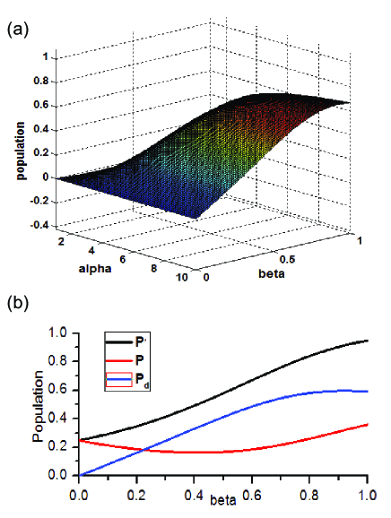
Figure 2: (Color online) (a) Schematic of the population difference $P_{d}$ varying with parameters $\alpha$ and $\beta$. (b) The populations $P$ (red), $P^{\prime}$ (black) and $P_{d}$ (blue) as functions of the parameter $\beta$ $(0\rightarrow 1.0)$ for the parameter $\alpha=6$.

To detect the non-Abelian nature, we first prepare the initial state as $|\psi\rangle_{i}=|D_{2}\rangle_{i}=|1\rangle$, and then let it undergo two closed paths $C_{1}$ and $C_{2}$ in different orders, i.e., $U=U_{2}U_{1}$ (first $C_{1}$ then $C_{2}$) and $U^{\prime}=U_{1}U_{2}$ (first $C_{2}$ then $C_{1}$). In order to implement the evolution $U(U^{\prime})$, let $U_{1}$ ($U_{2}$) in effect during time $-\tau\rightarrow\tau$, while $U_{2}$ ($U_{1}$) during time $\tau\rightarrow 3\tau$. The final states will be $|\psi\rangle_{f}=U|1\rangle=-U_{21}|2\rangle+U_{22}|1\rangle$, $|\psi\rangle^{\prime}_{f}=U^{\prime}|1\rangle=-U^{\prime}_{21}|2\rangle+U^{\prime}_{22}|1\rangle$, respectively. Therefore, the population difference $P_{d}$ of the two different final states in $|1\rangle$ is

$$P_{d}=P^{\prime}-P=|U^{\prime}_{22}|^{2}-|U_{22}|^{2}.$$ (14)

Whenever the $P_{d}\neq 0$ is detected, the noncommutative feature of the non-Abelian GP is verified. The population difference $P_{d}$ is numerically calculated with variables $\alpha$ and $\beta$, as shown in Fig. 2 (a), which obviously indicates that $P_{d}\neq 0$. Fig. 2 (b) is a specific plot of the population difference $P_{d}$ with $\beta$ as the only variable while $\alpha=6$, which shows maximum $P_{d}\approx 0.6$ when $\beta=0.9$.

Detecting the population difference of state $|1\rangle\equiv|0egg\rangle$ means that we just need to observe population difference on the excited state $|e\rangle$ of qubit 1, which can be realized by quantum non-demolition (QND) measurement. This can be achieved by tuning the qubit dispersively coupled to the cavity with a large detuning $\Delta$, and then measuring Hamiltonian will be $\hat{H}_{M}=\hbar(\omega+\chi\sigma_{z})a^{{\dagger}}a$ with $\chi=g^{2}/\Delta$. We can then get a different frequency shift $\pm\chi$ of the cavity mode with the qubit state on $|g\rangle$ and $|e\rangle$, respectively. With the coupling strength $g_{1}/2\pi=100$ MHz and the detuning $\Delta=5g$, we can get the frequency shift as $\chi/2\pi=20$ MHz, which is readily resolvable experimentally with high fidelity ARA .

In summary, we have proposed an experimentally feasible scheme to detect the noncommutative feature of the non-Abelian GP with effective tripod Hamiltonian in circuit QED. The non-Abelian nature of GP is verified by the fact that for an initial state undergoes the two specific loops in different order will lead to different final states. This differences is detected through observing the population difference of state $|0egg\rangle$, which is achieved QND measurement in circuit QED.

This work was supported by the NFRPC (No. 2013CB921804), the NSFC (No. 11004065), the PCSIRT, the NSF of Guangdong Province, and the Program of the Education Department of Anhui Province (No. KJ2012B075).

References

- (1) M. V. Berry, Proc. R. Soc. Lond. A 392, 45 (1984).
- (2) F. Wilczek and A. Zee, Phys. Rev. Lett. 52, 2111 (1984).
- (3) A. Carollo, I. Fuentes-Guridi, M. F. Santos, and V. Vedral, Phys. Rev. Lett. 90, 160402( 2003).
- (4) G. De Chiara and G. M. Palma, Phys. Rev. Lett. 91, 090404 (2003).
- (5) A. Carollo, I. Fuentes-Guridi, M. F. Santos, and V. Vedral, Phys. Rev. Lett. 92, 020402 (2004).
- (6) P. Solinas, P. Zanardi, and N. Zanghi, Phys. Rev. A 70, 042316 (2004).
- (7) I. Fuentes-Guridi, F. Girelli, and E. Livine, Phys. Rev. Lett. 94, 020503 (2005).
- (8) S.-L. Zhu and P. Zanardi, Phys. Rev. A 72, 020301(R) (2005).
- (9) S. Filipp et al., Phys. Rev. Lett. 102, 030404 (2009).
- (10) P. Zanardi and M. Rasetti, Phys. Lett. A 264, 94 (1999).
- (11) J. Pachos, P. Zanardi, and M. Rasetti, Phys. Rev. A 61, 010305 (1999).
- (12) J. A. Jones, V. Vedral, A. Ekert, and G. Castagnoli, Nature (London) 403, 869 (2000).
- (13) L.-M. Duan, J. I. Cirac, and P. Zoller, Science 292, 1695 (2001).
- (14) S.-L. Zhu and Z. D. Wang, Phy. Rev. Lett. 91, 187902 (2003).
- (15) S.-L. Zhu, Z.D. Wang, and P. Zanardi, Phys. Rev. Lett. 94, 100502 (2005); Z.-Y. Xue and Z. D. Wang, Phys. Rev. A 75, 064303 (2007); Z.-Y. Xue, Z. D. Wang, and S.-L. Zhu, Phys. Rev. A 77, 024301 (2008); Z.-Y. Xue, Quantum Inf. Process. 11, 1381 (2012).
- (16) R. Tycko, Phys. Rev. Lett. 58, 2281 (1987); J. Anandan, J. Christian, and K. Wanelik, Am. J. Phys. 65, 180 (1997).
- (17) P. J. Leek et al., Science 318, 1889 (2007); M. Möttönen, J. J. Vartiainen, and J. P. Pekola, Phys. Rev. Lett. 100, 177201 (2008).
- (18) D. Leibfried et al., Nature (London) 422, 412 (2003).
- (19) R. G. Unanyan, B. W. Shore, and K. Bergmann, Phys. Rev. A 59, 2910 (1999).
- (20) J. Ruseckas, G. Juzeliūnas, P. Öhberg, and M. Fleischhauer, Phys. Rev. Lett. 95, 010404 (2005).
- (21) X.-D. Zhang, Z. D.Wang, L.-B. Hu, Z.-M. Zhang, and S.-L. Zhu, New J. Phys. 10, 043031 (2008).
- (22) Y.-X. Du, Z.-Y. Xue, X.-D. Zhang, and H. Yan, Phys. Rev. A 84, 034103 (2011).
- (23) E. Sjöqvist, D. M. Tong, L. M. Andersson, B. Hessmo, M. Johansson and K. Singh, New J. Phys. 14, 103035 (2012); M. Johansson, E. Sjöqvist, L. M. Andersson, M. Ericsson, B. Hessmo, K. Singh, and D. M. Tong, Phys. Rev. A 86, 062322 (2012).
- (24) Z.-B. Feng, Y.-M. Zhang, G.-Z. Wang, and H. Han, Physica E 41, 1859 (2009).
- (25) J. Q. You and F. Nori, Nature 474, 589 (2011); Phys. Today 58(11), 42 (2005).
- (26) I. Buluta and F. Nori, Science 326, 108 (2009); I. Buluta, S. Ashhab, and F. Nori, Rep. Prog. Phys. 74, 104401 (2011).
- (27) R. J. Schoelkopf and S. M. Girvin, Nature (London) 451, 664 (2008).
- (28) A. Blais, R. S. Huang, A. Wallraff, S.M.Girvin, and R. J. Schoelkopf, Phys. Rev. A 69, 062320 (2004).
- (29) M. D. Reed et al., Nature (London) 482, 382 (2012); L. DiCarlo et al., Nature (London) 467, 574 (2010); M. Neeley et al., Nature (London) 467, 570 (2010).
- (30) I. Kamleitner, P. Solinas, C. Müller, A. Shnirman, and M. Möttönen, Phys. Rev. B 83, 214518 (2011).
- (31) J. Koch et al., Phys. Rev. A 76, 042319 (2007).
- (32) J. Q. You, X. Hu, S. Ashhab, and F. Nori, Phys. Rev. B 75, 140515(R) (2007).
- (33) P. K. Day, H. G. LeDuc, B. A. Mazin, A. Vayonakis, and J. Zmuidzinas, Nature (London) 425, 817 (2003).